On the Complexity of Randomly Weighted Multiplicative Voronoi Diagrams

Abstract

We provide an $O(n\operatorname{polylog}n)$ bound on the expected complexity of the randomly weighted multiplicative Voronoi diagram of a set of $n$ sites in the plane, where the sites can be either points, interior-disjoint convex sets, or other more general objects. Here the randomness is on the weight of the sites, not their location. This compares favorably with the worst case complexity of these diagrams, which is quadratic. As a consequence we get an alternative proof to that of Agarwal et al. [AHKS14] of the near linear complexity of the union of randomly expanded disjoint segments or convex sets (with an improved bound on the latter). The technique we develop is elegant and should be applicable to other problems.

1 Introduction

One of the fundamental structures in Computational Geometry is the Voronoi diagram [Aur91, AKL13]; that is, for a set of points ${P}$ in the plane, called sites, partition the plane into cells such that each cell is the locus of all the points in the plane whose nearest neighbor is a specific site in ${P}$. In the plane, the standard Voronoi diagram has linear combinatorial complexity, but in higher dimensions the complexity is $\Theta\left({n^{\left\lceil{d/2}\right\rceil}}\right)$. Many generalizations of this fundamental structure have been considered, including (i) adding weights, (ii) sites that are regions other than points, (iii) extensions to higher dimensions, (iv) other underlying metrics, and (v) many others.

Even in the plane, some of these generalizations of Voronoi diagrams lose their attractiveness as their complexity becomes quadratic in the worst case. However, as is often the case, constructions that realize the quadratic complexity (of say, the weighted multiplicative Voronoi diagram in the plane) are somewhat contrived, and brittle – little changes in the weight dramatically reduces the overall complexity. To quantify this observation, we consider here the expected complexity rather than the worst case of such diagrams, where weights are being assigned randomly.

Generalizations of Voronoi diagrams.

In the additive weighted Voronoi diagram, the distance to a Voronoi site is the regular Euclidean distance plus some constant (which depends on the site). Additive Voronoi diagrams have linear descriptive complexity in the plane, as their cells are star shaped (and thus simply connected), as can be easily verified. This holds even if the sites are arbitrary convex sets. In the multiplicative weighted Voronoi diagram, for each site one multiplies the Euclidean distance by a constant (again, that depends on the site). However, unlike the additive case, the worst case complexity for multiplicative weighted Voronoi diagrams is $\Theta(n^{2})$ [AE84], even in the plane. In the weighted case, the cells are not necessarily connected, and a bisector of two sites is either a line or an (Apollonius) circle.

In the Power diagram, each site ${s}_{i}$ has an associated radius $r_{i}$, and the distance of a point ${p}$ to this site is $\left\|{{s}_{i}}-{{p}}\right\|^{2}-r_{i}^{2}$; that is, the squared length of the tangent from ${p}$ to the disk of radius $r_{i}$ centered at ${s}_{i}$. As such, Power diagrams allow including weight in the distance function, while still having bisectors that are straight lines and having linear combinatorial complexity overall.

Klein [Kle88] introduced (and this was further refined by Klein et al. [KLN09]) the notion of abstract Voronoi diagrams to help unify the ever growing list of variants of Voronoi diagrams which have been considered. Specifically, a simple set of axioms was identified, focusing on the bisectors and the regions they define, which classifies a large class of Voronoi diagrams with linear complexity (hence such axioms are not intended to model, for example, multiplicative diagrams).

Randomization and Expected Complexity.

In many cases, there is a big discrepancy between the worst case analysis of a structure (or an algorithm) and its average case behavior. This suggests that in practice, the worst case is seldom encountered. For example, recently, Agarwal et al. [AKS13, AHKS14], showed that the expected union complexity of a set of randomly expanded disjoint segments is $O(n\log n)$, while in the worst case the union complexity can be quadratic. In other words, Agarwal et al. bounded the expected complexity of a level set of the randomly weighted Voronoi diagram of disjoint segments.

If the sites are placed randomly.

There is extensive work on the expected complexity of various structures (including Voronoi diagrams) if the sites are being picked randomly (but not their weight), see [San53, RS63, Ray70, Dwy89, WW93, SW93, OBSC00, Har11b, DHR12] (this list is in no way exhaustive). In many of these cases the resulting expected complexity is dramatically smaller than its worst case analysis. For example, in ${\rm I\!R}^{d}$, the Voronoi diagram of $n$ sites picked uniformly inside a hypercube has $O(n)$ complexity (the constant depends exponentially on the dimension), but the worst case complexity is, as already mentioned, $\Theta(n^{\left\lceil{d/2}\right\rceil})$. Intuitively, the low complexity when the locations are randomly sampled is the result of the relative uniformity of such samples. Interestingly, there is a subtle connection between such settings and the behavior of grid points [Har98].

However, in this paper, site locations will be fixed and site weights will be sampled (similar to the model of Agarwal et al. [AHKS14]). As such, our argument cannot rely on the spacial uniformity provided by location sampling. Nevertheless, the case of fixed (distinct) weights and sampled locations will follow readily from our arguments for the sampled weights and fixed locations case, see Section 5.1.2.

Technical Challenges in the Multiplicative Setting.

In this paper, we focus on the case of multiplicative weighted Voronoi diagrams in the plane. As mentioned above, such diagrams can have quadratic complexity. It is thus natural to consider sampling (of the weights) as a way to mitigate this, and argue for lower expected complexity. However, the multiplicative case poses a significant technical hurdle in that nearest weighted neighbor relations are a non-local phenomena. Specifically, for a given site, unless all its neighbors (in the unweighted diagram) have lower weight, its region of influence cannot be locally contained, and its cell spills over – potentially affecting points far away. This non-locality makes arguing about such diagrams technically challenging. For example, the work of Agarwal et al. [AHKS14] required quite a bit of effort to bound the level set of the multiplicative Voronoi diagram for segments, and it is unclear how their analysis can be extended to bound the complexity of the whole diagram.

Our Results.

Consider a fixed distribution from which we sample weights. Our main result is that the expected complexity of the multiplicative weighted Voronoi diagram of a set of sites is near linear, where the sites are disjoint simply-connected compact regions in the plane. We specify the exact requirements on the sites in Section 2 — possible sites include points, segments, or convex sets.

A simple consequence of our main result is that the expected complexity of the union of randomly expanded disjoint segments or convex sets is also near linear. Specifically, our proof is significantly simpler than the one of Agarwal et al. [AHKS14]. Our bound is weaker by (roughly) an $O(\log n)$ factor for the case of segments, but for convex sets we improve the bound from $O(n^{1+\varepsilon})$ to $O(n\operatorname{polylog}n)$ (and our bound holds for the complexity of the whole diagram, not only the level set). Also, similar to the work of Agarwal et al., in Section 5.1.1 we make the observation that our results also hold for the more general case where instead of sampling weights from a distribution, one is given a fixed set of $n$ weights which are randomly permuted among the sites.

Our technique is rather versatile and should be applicable to other well behaved distance metrics (for example, when each site has its own additive constant which is included when measuring the distance to that site).

To extend our result to more general sites, we prove that in these settings the expected complexity of the overlay of the Voronoi cells in a randomized incremental construction is $O(\lambda_{\psi}\left({n}\right)\log n)$ (see Lemma 4.5${}_{\text{p\ref{lemma:overlay:2}}}$), where $\lambda_{\psi}\left({n}\right)$ is the length of a Davenport-Schinzel sequence of order $\psi$ with $n$ symbols, where $\psi$ is some constant. This is an extension of the result of Kaplan et al. [KRS11] to these more general settings.

Significance of Results.

As discussed above, due to non-locality, analyzing multiplicative diagrams seems challenging. In particular, we are unaware of any previous subquadratic bounds for the expected complexity. On the practical side, the unwieldy complexity of the multiplicative diagram (and its lack of a dual structure, similar to Delaunay triangulations) has discouraged their use in favor of more well behaved diagrams, such as the power diagram. Our work indicates that using such diagrams in the real world might be practical, despite their worst case quadratic complexity. In particular, our technique for bounding the expected complexity immediately implies a near linear time randomized incremental construction algorithm for computing the multiplicative diagram.

Outline of technique.

Consider the case of bounding the expected complexity of the Voronoi diagram of a set ${P}$ of $n$ multiplicatively weighted points (i.e., sites) in the plane, where the weights are being picked independently from the same distribution. The key ideas behind the new approach are the following.

1. Candidate Sets. Consider any point ${x}$ in the plane, and let ${p}$ be its nearest neighbor in ${P}$ under the weighted distance. Now, if ${p}$ is the nearest neighbor of ${x}$ then for all other sites in ${P}$ either ${p}$ has smaller weight, or smaller distance to ${x}$. Thus for each point ${x}$ in the plane one can define its candidate set, which consists of all sites ${z}\in{P}$ such that for all other sites in ${P}$ either ${z}$ has smaller weight or smaller distance to ${x}$. Saying it somewhat differently, plotting the points of ${P}$ in the parametric plane, where one axis is the distance from ${x}$, and the other axis is their weight, the candidate set is all the minima points (i.e., they are the vertices of the lower left staircase of the point set, and they are not dominated in both axes by any other point). We show that when weights are randomly sampled, with high probability, for all points in the plane the candidate set has at most logarithmic size (this is well known, and we include the proof for the sake of completeness).

2. Gerrymandering the plane. Next, we partition the plane into a small number of regions such that the candidate set is fixed within each region. Specifically, if one can break the plane into $m$ such uniform candidate regions, then the worst case complexity of the Voronoi diagram is $O(m\log^{2}n)$, with high probability, since all candidate sets are of size at most $O(\log n)$, and the worst case complexity of the multiplicative Voronoi diagram of a weighted set of points is quadratic.

3. Randomized Incremental Campaigning. The main challenge, as frequently is the case, is to do the gerrymandering. To this end, consider adding the sites in order of increasing weight. When the $i$th site is added, it has higher weight than the sites already added, and lower weight than the sites which have not been added yet. Therefore, the $i$th site is in the candidate set of a point in the plane, when it is the nearest neighbor of the point among the first $i$ sites. In other words, the points in the Voronoi cell of the $i$th site in the Voronoi diagram of the first $i$ sites. Next, consider the overlay of the $n$ Voronoi cells formed by taking all $i\in\left\{{1,\ldots,n}\right\}$. Observe that each face of this overlay has the same candidate set. For the case of points, Kaplan et al. [KRS11] proved that this overlay has $O(n\log n)$ expected complexity. This implies immediately an $O(n\log^{3}n)$ bound on the expected complexity of the multiplicative Voronoi diagram.

Organization.

In Section 2 we introduce notation and definitions used throughout the paper. In Section 3 we introduce the notion of candidate sets, and show how partitioning the plane into a near linear number of regions, such that each region has the same candidate set implies our result on the near linear expected complexity of the multiplicative Voronoi diagram of sites. Specifically, the partitioning used is the overlay of Voronoi cells in a randomized incremental construction (RIC), and in Section 4 we describe in detail how the expected complexity of such an overlay is near linear. In Section 5 we state our main result, and present a number of specific applications of our technique. In Section 5.1.1 we observe that instead of sampling weights our technique extends to the more general case of permuting a fixed set of weights among the points. In Appendix A, we show that the overlay of Voronoi cells in RIC is $\Omega(n\log n)$, implying that the upper bound of Kaplan et al. [KRS11] is tight in this case.

2 Preliminaries

Below we define Voronoi diagrams and related objects in a rather general way to encompass the various applications of our technique. For simplicity the reader is encouraged to interpret these definitions in terms of Voronoi diagrams of points (or less trivially disjoint segments).

Notation.

We use ${T}=\left\langle{{s}_{1},\ldots,{s}_{n}}\right\rangle$ to denote a permutation of a set ${S}$ of $n$ objects, and ${T}_{i}=\left\langle{{s}_{1},\ldots,{s}_{i}}\right\rangle$ to denote the prefix of this permutation of length $i$. Similarly, we use ${T}_{i+1}^{n}=\left\langle{{s}_{i+1},{s}_{i+2},\ldots,{s}_{n}}\right\rangle$ to denote a suffix of ${T}$. When we care only about what elements appear in a permutation, ${T}$, but not their internal ordering, we use the notation ${S}=\mathrm{set}\left({{T}}\right)$ to denote the associated set. As such, ${S}_{i}=\mathrm{set}\left({{T}_{i}}\right)$ is the unordered prefix of length $i$ of ${T}$, and ${S}_{i+1}^{n}=\mathrm{set}\left({{T}_{i+1}^{n}}\right)=\left\{{{s}_{i+1},{s}_{i+2},\ldots,{s}_{n}}\right\}$ is the unordered suffix.

Arrangements.

As it will be used throughout the paper, we now define the standard terminology of arrangements (see [SA95, Har11a]). Given a set $\mathsf{S}$ of $n$ segments in the plane, its arrangement, denoted by $\mathcal{A}(\mathsf{S})$, is the decomposition of the plane into faces, edges and vertices. The vertices $\mathcal{A}(\mathsf{S})$ are the endpoints and the intersection points of the segments of $\mathsf{S}$, the edges are the maximal connected portions of the segments not containing any vertex, and the faces are the connected components of the complement of the union of the segments of $\mathsf{S}$. For a set of polygons, we can analogously define its arrangement by letting $\mathsf{S}$ be the union of all boundary segments of the polygons.

2.1 Voronoi diagrams

Let ${S}=\left\{{{s}_{1},\ldots,{s}_{n}}\right\}$ be a set of $n$ sites in the plane. Specifically, the sites are disjoint simply-connected compact subsets of ${\rm I\!R}^{2}$. For a closed set $Y\subseteq{\rm I\!R}^{2}$, and any point ${x}\in{\rm I\!R}^{2}$, let $\mathsf{d}\left({{x},Y}\right)=\min_{y\in Y}\left\|{x}-y\right\|$ denote the distance of ${x}$ to the set $Y$. For any two sites ${s},{r}\in{S}$, we define their bisector $\beta({s},{r})$ as the set of points ${x}\in{\rm I\!R}^{2}$ such that $\mathsf{d}\left({{x},{s}}\right)=\mathsf{d}\left({{x},{r}}\right)$. Each ${s}\in{S}$, induces the function $f_{s}({x})=\mathsf{d}\left({{x},{s}}\right),$ where ${x}$ is any point in the plane. For any subset ${H}\subseteq{S}$ and any site ${s}\in{H}$, the Voronoi cell of ${s}$ with respect to ${H}$, denoted $\mathcal{V}_{\mathrm{cell}}\left({{s},{H}}\right)$, is the subset of ${\rm I\!R}^{2}$ whose closest site in ${H}$ is ${s}$, i.e. $\mathcal{V}_{\mathrm{cell}}\left({{s},{H}}\right)=\left\{{x}\in{\rm I\!R}^{2}\;\middle|\;\forall{r}\in{H}\;\;f_{s}({x})\leq f_{r}({x})\right\}\Bigr{.}.$ Finally, for any subset ${H}\subseteq{S}$, the Voronoi diagram of ${H}$, denoted $\mathcal{V}\left({{H}}\right)$, is the partition of the plane into Voronoi cells induced by the minimization diagram of the set of functions $\left\{f_{s}\;\middle|\;\bigl{.}{s}\in{H}\right\}$.

Remark 2.1.

Throughout the paper we require the following from the bisectors and Voronoi cells.

1. For any two sites ${s},{r}\in{S}$, their bisector $\beta({s},{r})$ is a simple curve (i.e. the image of a continuous map from the unit interval to ${\rm I\!R}^{2}$) whose removal splits the plane into exactly two unbounded regions.

2. Each bisector is of constant complexity, that is it has a constant number of extremal points in the direction of (say) the $x$-axis.

3. Any two distinct bisectors intersect at most a constant number of times.

4. For any site ${s}\in{S}$ and any subset ${H}\subseteq{S}$, the set $\mathcal{V}_{\mathrm{cell}}\left({{s},{H}}\right)$ is a simply connected subset of the plane.

5. For any subset ${H}\subseteq{S}$, the Voronoi cells cover the plane; that is, $\cup_{{s}\in{H}}\,\mathcal{V}_{\mathrm{cell}}\left({{s},{H}}\right)={\rm I\!R}^{2}$.

One can view the union, $U$, of the boundaries of the cells in a Voronoi diagram as a planar graph. Specifically, define a Voronoi vertex as any point in $U$ which is equidistant to three sites in ${S}$ (which happens at the intersection of two bisectors). For simplicity, we make the general position assumption that no point is equidistant to four or more sites in the plane. Furthermore, define a Voronoi edge as any maximal connected subset of $U$ which does not contain a Voronoi vertex. (Note that in order for each edge to have two endpoints we must include the “point” at infinity, i.e. the graph is defined on the stereographic projection of the plane onto the sphere.)

The above conditions imply that the Voronoi diagram of any subset of sites is an abstract Voronoi diagram (actually such diagrams are more general). It is known that for such diagrams the overall complexity of the Voronoi graph they define is linear [KLN09], i.e. for a set of $n$ sites the number of Voronoi vertices, edges, and faces is $O(n)$. In general Voronoi diagrams, edges may have more than a constant number of $x$-extremal points. However, since we assumed each bisector has a constant number of $x-$extremal points, and Voronoi edges are contiguous subsets of bisectors, there are only a constant number of $x$-extremal points on any edge. Therefore, asymptotically, the complexity of the vertical decomposition of the Voronoi diagram, and thus the diagram itself, is bounded by the complexity of this (Voronoi) graph.

2.2 Multiplicative weighted Voronoi diagrams

As before, let ${S}$ be a set of $n$ weighted sites in the plane, where $\omega_{i}>0$ is the weight associated with the $i$th site ${s}_{i}$. Consider the weighted Voronoi diagram of ${S}$, denoted by $\mathcal{W}\left({{S}}\right)$. Specifically, for $i=1,\ldots,n$, the site ${s}_{i}$ induces a distance function $f_{i}({x})=\omega_{i}\,\mathsf{d}\left({{x},{s}}\right)$. The multiplicative weighted Voronoi diagram of ${S}$ is the partition of the plane induced by the minimization diagram of the distance functions $f_{1},\ldots,f_{n}$. The weighted Voronoi cell of ${s}_{i}$ is

$$C_{i}=\left\{{x}\in{\rm I\!R}^{2}\;\middle|\;\forall j\quad f_{i}({x})\leq f_{j}({x})\right\}.$$ (2.1)

For a multiplicative Voronoi diagram, the cells are not necessarily connected.

Remark 2.2.

In addition to the conditions listed in Remark 2.1, for the unweighted case, we also require the following of the weighted diagram (for any positive weight assignment):

1. Each weighted bisector has a constant number of extremal points in the direction of the $x$-axis.

2. Any two distinct weighted bisectors intersect at most a constant number of times.

Let $g\left({n}\right)$ denote the worst case complexity of the multiplicative weighted Voronoi diagram. The analysis below requires a polynomial bound on $g\left({n}\right)$. It is not hard to see that the conditions above on bisectors already imply a bound of $g\left({n}\right)=O(n^{4})$.

2.2.1 Assigning weights randomly

In the following, we use distribution to refer to any probability distribution defined over the positive real numbers (i.e., ${\rm I\!R}^{+}$). We use $\xi$ to denote this distribution, which might be continuous or discrete.

Let ${S}$ be a given set of $n$ sites in the plane. We assign each site of ${S}$ a random weight sampled independently from $\xi$. We order the sites of ${S}$ by their weight, and let ${s}_{i}$ be the site assigned the $i$th smallest weight, and let $\omega_{i}$ denote this weight, for $i=1,\ldots,n$. If the weights assigned are not unique, we randomly permute each cluster of sites that are assigned the same weight internally. The resulting ordering ${T}=\left\langle{{s}_{1},\ldots,{s}_{n}}\right\rangle$ is a (uniform) random permutation defined over the sites of ${S}$.

3 Bounding the complexity of the randomly weighted diagram

Let ${S}$ be a weighted set of sites in the plane, whose ordering by increasing weight is ${T}=\left\langle{{s}_{1},\ldots,{s}_{n}}\right\rangle$ (where $\omega_{i}$ is the weight of ${s}_{i}$). For any point ${x}\in{\rm I\!R}^{2}$, we write ${\mathop{{\mathcal{W}}_{\mathrm{cell}}}\left({{x},{S}}\right)}$ to denote the Voronoi cell of $\mathcal{W}\left({{S}}\right)$ that contains ${x}$, i.e. ${\mathop{{\mathcal{W}}_{\mathrm{cell}}}\left({{x},{S}}\right)}=C_{i}$ is induced by the site ${s}_{i}=\arg\min_{{s}_{j}\in{S}}\omega_{j}\left\|{x}-{s}_{j}\right\|$, see Eq. (2.1) (if ${x}$ is a boundary point, then we arbitrarily pick one of the equidistant sites).

3.1 Candidate sets

Definition 3.1.

Let ${T}=\left\langle{{s}_{1},\ldots,{s}_{n}}\right\rangle$ be an ordered set of $n$ sites in the plane. For any point ${x}$ in the plane, the candidate set of ${x}$, denoted by ${L}\left({{x},{T}}\right)$, is the set of all sites ${s}_{i}\in{T}$, such that $\left\|{x}-{s}_{i}\right\|=\mathsf{d}\left({{x},{T}_{i}}\right)$, for $i=1,\ldots,n$. In words, ${s}_{i}$ is in ${L}\left({{x},{T}}\right)$ if it is the closest site to ${x}$ in its prefix ${T}_{i}$.

A prerequisite for a site ${s}_{j}$ of the weighted site set ${S}$ to be the nearest site under weighted distances to ${x}$, is that ${s}_{j}$ is in the candidate set ${L}\left({{x},{T}}\right)$.

Lemma 3.2.

For a point ${x}$ in the plane, if $\,{\mathop{{\mathcal{W}}_{\mathrm{cell}}}\left({{x},{S}}\right)}=C_{j}$, then ${s}_{j}$ is in ${L}\left({{x},{T}}\right)$, where ${T}$ is the ordering of ${S}$ by increasing weight.

Proof:

Let ${s}_{j}$ be the nearest weighted site to ${x}$ (in the weighted Voronoi diagram of ${S}$). Consider any other site ${s}_{i}$ such that $\omega_{i}<\omega_{j}$. This implies that $i<j$ because of the ordering of ${T}$. Observe that ${s}_{i}$ is further away from ${x}$ than ${s}_{j}$ (i.e., $\left\|{x}-{s}_{j}\right\|<\left\|{x}-{s}_{i}\right\|$), since otherwise

$$f_{j}\left({{x}}\right)=\omega_{j}\left\|{x}-{s}_{j}\right\|\geq\omega_{j}\left\|{x}-{s}_{i}\right\|>\omega_{i}\left\|{x}-{s}_{i}\right\|=f_{i}\left({{x}}\right),$$

which is a contradiction. In other words, ${s}_{j}$ must be the (unweighted) closest point to ${x}$ in its prefix ${T}_{j}$.  

We next prove that, with high probability, the candidate set is logarithmic in size for all points in the plane. To this end, we need the following helper lemma.

Lemma 3.3.

Let $\Pi=\left\langle{\pi_{1},\ldots,\pi_{n}}\right\rangle$ be a random permutation of $\left\{{1,\ldots,n}\right\}$, and let $X_{i}$ be an indicator variable which is $1$ if $\pi_{i}$ is the smallest number among $\pi_{1},\ldots,\pi_{i}$, for $i=1,\ldots,n$. Let $Z=\sum_{i=1}^{n}X_{i}$, then $Z=O(\log n)$, with high probability (i.e., $\geq 1-1/n^{c}$, for any constant $c$).

Proof:

This is well known [Mul94, Section 3.4], and we include the proof for the sake of completeness. Let $\mathcal{E}_{i}$ be the event that $X_{i}=1$, for $i=1,\ldots,n$. We first show the events $\mathcal{E}_{1},\ldots,\mathcal{E}_{n}$ are independent (implying the $X_{i}$ are independent). Indeed, conceptually, generate the permutation as follows: Randomly pick a permutation of the given numbers, and set the first number to be $\pi_{n}$. Next, pick a random permutation of the remaining numbers and set the first number as the penultimate number (i.e., $\pi_{n-1}$) in the output permutation. Repeat this process till we generate the whole permutation.

Observe that by our thought experiment, regardless of the elements that appear in the suffix $\left\langle{\pi_{i_{1}+1},\ldots,\pi_{n}}\right\rangle$, there is exactly one minimum value in the remaining elements, and these remaining elements are randomly permuted before determining $\pi_{i}$. Now, consider arbitrary indices $1\leq i_{1}<i_{2}<\ldots<i_{k}\leq n$. Clearly, the event $\mathcal{E}_{i+1}$ is not influenced by the exact choice of the suffix $\pi_{i+1},\ldots,\pi_{n}$, and as such $\mathop{\mathbf{Pr}}\!\left[{\mathcal{E}_{i_{1}}\!\,\left|\,{\pi_{i_{1}+1},\ldots,\pi_{n}}\bigr{.}\right.}\right]=\mathop{\mathbf{Pr}}\!\left[{\bigl{.}\mathcal{E}_{i_{1}}}\right]=1/i_{1}.$ Furthermore, we have $\mathop{\mathbf{Pr}}\!\left[{\mathcal{E}_{i_{1}}\,\left|\,{\mathcal{E}_{i_{2}}\cap\ldots\cap\mathcal{E}_{i_{k}}}\bigr{.}\right.}\right]=\mathop{\mathbf{Pr}}\!\left[{\bigl{.}\mathcal{E}_{i_{1}}}\right]=1/i_{1}$ as can be easily verified. As such, by induction, we have

$$\mathop{\mathbf{Pr}}\!\left[{\bigl{.}\bigcap\nolimits_{j=1}^{k}\mathcal{E}_{i_{j}}}\right] =\mathop{\mathbf{Pr}}\!\left[{\bigl{.}\mathcal{E}_{i_{1}}\,\left|\,{\bigcap\nolimits_{j=2}^{k}\mathcal{E}_{i_{j}}}\bigr{.}\right.}\right]\mathop{\mathbf{Pr}}\!\left[{\bigcap\nolimits_{j=2}^{k}\mathcal{E}_{i_{j}}}\right]=\mathop{\mathbf{Pr}}\!\left[{\bigl{.}\mathcal{E}_{i_{1}}}\right]\Bigl{.}\mathop{\mathbf{Pr}}\bigl{[}\bigcap\nolimits_{j=2}^{k}\mathcal{E}_{i_{j}}\bigr{]}\biggr{.}=\prod_{j=1}^{k}\mathop{\mathbf{Pr}}\!\left[{\mathcal{E}_{i_{j}}}\right]=\prod_{j=1}^{k}\frac{1}{i_{j}}.$$

We conclude that the variables $X_{1},\ldots,X_{n}$ are independent. The claim now follows from the Chernoff bound since $\mu=\mathop{\mathbf{E}}\!\left[{\bigl{.}Z}\right]=\sum_{i}\Bigl{.}\mathop{\mathbf{E}}\!\left[{\bigl{.}X_{i}}\right]=\sum_{i=1}^{n}{1}/{i}=\Theta(\log n).$  

Corollary 3.4.

Let ${S}$ be a randomly weighted set of $n$ sites in the plane, and let ${T}=\left\langle{{s}_{1},\ldots,{s}_{n}}\right\rangle$ be the sorted ordering of ${S}$ by increasing weight. Simultaneously for all points in the plane their candidate set for ${T}$ is of size $O(\log n)$, with high probability.

Proof:

Consider any fixed point ${x}$ in the plane. Since ${T}=\left\langle{{s}_{1},\ldots,{s}_{n}}\right\rangle$ is a random permutation of ${S}$, the sequence $\left\|{x}-{s}_{1}\right\|,\ldots,\allowbreak\left\|{x}-{s}_{n}\right\|$ is a random permutation of the distance values from ${x}$ to the sites in ${S}$. Therefore, by the definition of the candidate set and Lemma 3.3, we have $\left|{{L}\left({{x},{T}}\right)}\right|=O(\log n)$ with high probability.

Consider the arrangement of all the (unweighted) bisectors of all the pairs of sites in ${S}$. There are $n$ sites and $\binom{n}{2}$ bisectors. As such, there are $O\left({n^{4}}\right)$ vertices in this arrangement, as by assumption each pair of bisectors intersect at most a constant number of times, and each bisector has a constant number of $x$-extremal points. Therefore, the total complexity of this arrangement is $O\left({n^{4}}\right)$.

Within each face of this arrangement, the candidate set cannot change since all points in this face have the same ordering of their distances to the sites in ${S}$. So pick a representative point for each of the $O(n^{4})$ faces. For any such representative, with probability $\leq 1/n^{c}$, the candidate set has $>\alpha\log(n)$ sites, for any constant $c$ of our choosing (where $\alpha$ is a constant determined by the Chernoff bound that depends only on $c$). Therefore, by choosing $c$ to be sufficiently large, taking the union bound on these bad events, and then taking the complement, the claim follows.  

3.2 Getting a compatible partition

The goal now is to find a low complexity subdivision of the plane, such that within each cell of the subdivision the candidate set is fixed. The main insight is that by using the unweighted Voronoi diagram one can get such a subdivision.

Let $K_{i}$ denote the Voronoi cell of ${s}_{i}$ in the unweighted Voronoi diagram of the $i$th prefix ${S}_{i}=\left\{{{s}_{1},\ldots,{s}_{i}}\right\}$. Let $\mathcal{A}$ denote the arrangement formed by the overlay of the regions $K_{1},\ldots,K_{n}$. The complexity of $\mathcal{A}$, denoted by $\left|{\mathcal{A}}\right|$, is the total number of these faces, edges, and vertices, as well as the number of $x$-extremal points on the edges. By our assumptions on the bisectors, the number of vertices bounds the complexity $\left|{\mathcal{A}}\right|$.

Lemma 3.5.

For any face $F$ of $\mathcal{A}=\mathcal{A}\left({K_{1},\ldots,K_{n}}\right)$, the candidate set is the same, for all points in $F$.

Proof:

Initially, all points in the plane have the same candidate set, namely the empty set. When the site ${s}_{i}$ is added, the only points in the plane whose candidate set changes are those such that ${s}_{i}$ is their nearest neighbor in ${S}_{i}$. However, these are precisely the points in the Voronoi cell of ${s}_{i}$ in the unweighted Voronoi diagram of ${S}_{i}$. That is, the candidate set changes only for the points covered by $K_{i}$ – where ${s}_{i}$ is being added to the candidate set.

The claim now easily follows, as $\mathcal{A}$ is the overlay arrangement of these regions.  

Theorem 3.6.

Let ${S}$ be a set of $n$ sites in the plane, satisfying the conditions in Remark 2.1 and Remark 2.2, where for each site a weight is sampled independently from some distribution $\xi$. Let ${T}=\left\langle{{s}_{1},\ldots,{s}_{n}}\right\rangle$ be the ordering of the sites by increasing weights, and let $K_{i}=\mathcal{V}_{\mathrm{cell}}\left({{s}_{i},{T}_{i}}\right)$, for $i=1,\ldots,n$. Let $\mathcal{A}=\mathcal{A}\left({K_{1},\ldots,K_{n}}\right)$ be the arrangement formed by the overlay of all these cells.

Then, the expected complexity of the multiplicative Voronoi diagram $\mathcal{W}\left({{S}}\right)$ is $O\left({\Bigl{.}\mathop{\mathbf{E}}\!\left[{\bigl{.}\left|{\mathcal{A}}\right|}\right]g\left({\log n}\right)}\right)$, where $\left|{\mathcal{A}}\right|$ is the total complexity of $\mathcal{A}$, and $g\left({m}\right)$ denotes the worst case complexity of a weighted Voronoi diagram of $m$ sites.

Proof:

We first compute a vertical decomposition of the faces of $\mathcal{A}$, in order to break up each face into constant complexity cells. Specifically, each face has two types of vertices – extremal points on the bisectors and intersections of bisectors. From each such vertex shoot out vertical rays. Doing so partitions the plane into constant complexity cells (or, somewhat imprecisely, vertical trapezoids) and the total number of such cells is proportional to $\left|{\mathcal{A}}\right|$ (i.e. the number of extremal points and intersections).

Lemma 3.5 implies that within each cell of the vertical decomposition the candidate set is fixed. So consider such a cell $\Delta$, and let ${L}$ be its candidate set. Lemma 3.2 implies that the only sites whose weighted Voronoi cells can have non-zero area in $\Delta$ are the sites in ${L}$. That is, the Voronoi diagram in $\Delta$ is the intersection of $\Delta$ with the weighted Voronoi diagram of some subset of ${L}$. Now the weighted Voronoi diagram of $\leq\left|{{L}}\right|$ points has worst case complexity $g\left({\left|{{L}}\right|}\right)$. Since $\Delta$ is a constant complexity region this implies that the complexity of the weighted Voronoi diagram in $\Delta$ is $O\left({g\left({\left|{{L}}\right|}\right)}\right)$.

By Corollary 3.4, for all points in the plane, the candidate set is of size $O(\log n)$ (with high probability), and since there are $O(\left|{\mathcal{A}}\right|)$ cells (in expectation), the claim now readily follows.  

$n=2$	$n=3$	$n=4$
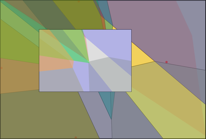
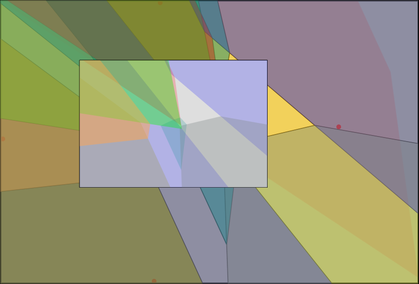
$n=5$	$n=6$	$n=7$
$n=8$	$n=9$	$n=10$

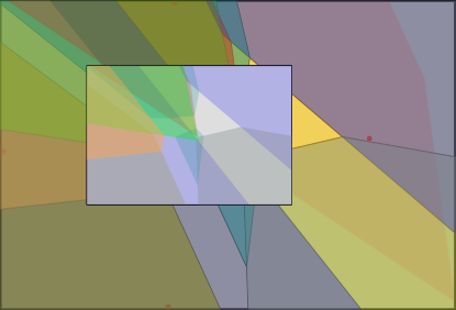
Figure 3.1: The randomized incremental construction of a Voronoi diagram of point sites, and the resulting overlay arrangement.

For the concrete case when the sites are points in the plane, the worst case complexity of the weighted Voronoi diagram is quadratic [AE84], and so in the above theorem $g\left({m}\right)=O(m^{2})$. Kaplan et al. [KRS11] showed that for a random permutation of $n$ points (as is the case here) the expected total complexity of $\mathcal{A}$ is $O(n\log n)$, see Figure 3.1 for an example of such an overlay arrangement. We therefore readily have the following result.

Theorem 3.7.

Let ${P}$ be a set of $n$ points in the plane, where for each point we independently sample a weight from some distribution $\xi$. Then the expected complexity of the multiplicative Voronoi diagram of ${P}$ is $O\left({n\log^{3}n}\right)$.

Corollary 3.8.

Let ${P}$ be a set of $n$ points in the plane, where for each point we independently sample a weight from some distribution $\xi$. Then the multiplicative Voronoi diagram of ${P}$ can be computed in $O\left({n\log^{3}n}\right)$ expected time.

Proof:

This follows readily from the above constructive proof, and so we only sketch the algorithm. First, compute the ordering ${T}=\left\langle{{s}_{1},\ldots,{s}_{n}}\right\rangle$ of the sites by increasing weight, and the set of polygons $\left\{{K_{1},\ldots,K_{n}}\right\}$, where $K_{i}=\mathcal{V}_{\mathrm{cell}}\left({{s}_{i},{T}_{i}}\right)$, by computing the unweighted Voronoi diagram by incremental construction (i.e. each $K_{i}$ is computed explicitly during the insertion of ${s}_{i}$). Next, compute $\mathcal{A}=\mathcal{A}\left({K_{1},\ldots,K_{n}}\right)$. Triangulate the faces of $\mathcal{A}$, and within each triangle compute the multiplicative Voronoi diagram of its candidate list, and clip it to the triangle (note the candidate lists are given by $\mathcal{A}$).

For the running time, computing the unweighted Voronoi diagram by randomized incremental construction takes $O(n\log n)$ expected time. By Kaplan et al. [KRS11], the total number of segments over all the polygons and the arrangement $\mathcal{A}$ have expected complexity $O(n\log n)$. Therefore computing $\mathcal{A}$ from $\left\{{K_{1},\ldots,K_{n}}\right\}$ takes $O(n\log^{2}n)$ expected time [Mul94]. Triangulating the faces takes linear time in $\left|{\mathcal{A}}\right|$. Using the quadratic time algorithm of Aurenhammer [Aur87], computing the multiplicative diagram in each face take $O(\log^{2}n)$ time, as by Corollary 3.4, all candidate lists have size $O(\log n)$.  

For more general sites, the real difficulty is in bounding $\mathop{\mathbf{E}}\!\left[{\left|{\mathcal{A}}\right|}\right]$. Specifically, in the next section we extend the result of Kaplan et al. [KRS11] to these more general settings.

4 The complexity of the overlay of Voronoi cells in RIC

We next study the expected complexity of the overlay of Voronoi cells and envelopes in a randomized incremental construction. Specifically, we first prove a result on the lower envelope of functions in two dimensions, and then use it to prove a bound on the complexity of the overlay of Voronoi cells of sites in the plane.

4.1 Preliminaries

In the following, we need to use the Clarkson-Shor technique [CS89], which we quickly review here (see [Har11a] for details). Specifically, let ${S}$ be a set of elements such that any subset ${R}\subseteq{S}$ defines a corresponding set of objects $\mathcal{T}\left({{R}}\right)$ (e.g., ${S}$ is a set of points or sites in the plane, and any subset $R\subseteq{S}$ induces the set of edges of the Voronoi diagram $\mathcal{V}\left({{R}}\right)$). Each potential object, $\tau$, has a defining set and a stopping set. The defining set, $D\left({\tau}\right)$, is a subset of ${S}$ that must appear in ${R}$ in order for the object to be present in $\mathcal{T}\left({{R}}\right)$, where this set has size bounded by the same constant for all objects. The stopping set, $\kappa\left({\tau}\right)$, is a subset of ${S}$ such that if any of its members appear in ${R}$ then $\tau$ is not present in $\mathcal{T}\left({{R}}\right)$ (we also naturally require that $\kappa\left({\tau}\right)\cap D\left({\tau}\right)=\emptyset$, for all $\tau$). Surprisingly, this already implies the following.

Theorem 4.1 (Bounded Moments, [CS89]).

Using the above notation, let ${S}$ be a set of $n$ elements, and let ${R}$ be a random sample of size $r$ from ${S}$. Let $f(\cdot)$ be a polynomially growing function. We have that $\displaystyle\mathop{\mathbf{E}}\!\left[{\sum\nolimits_{\tau\in\mathcal{T}\left({{R}}\right)}f\left({\bigl{.}\left|{\kappa\left({\tau}\right)}\right|}\right)}\right]=O\left({\Bigl{.}\mathop{\mathbf{E}}\!\left[{\bigl{.}\left|{\mathcal{T}\left({{R}}\right)}\right|}\right]f(n/r)}\right),$ where the expectation is over the sample ${R}$.

4.2 Complexity of the overlay of lower-envelopes of functions in RIC

Let $\mathcal{F}$ be a set of $n$ functions, such that for all $f\in\mathcal{F}$, we have (1) $f:{\rm I\!R}\rightarrow{\rm I\!R}$, and (2) $f$is continuous. The curve associated with $f$ is its image $\left\{{(x,f(x))\,\left|\,{x\in{\rm I\!R}}\bigr{.}\right.}\right\}$. We use $f$ to refer both to the function and its curve.

We assume that any pair of curves in $\mathcal{F}$ only intersect transversally and at most $\psi$ times, and that no three curves intersect at a common point (i.e. general position), where $\psi$ is some small constant. Here $\mathcal{G}=\left\langle{f_{1},\ldots,f_{n}}\right\rangle$ denotes a fixed permutation of the $n$ functions, $\mathcal{G}_{i}=\left\langle{f_{1},\ldots,f_{i}}\right\rangle$ denotes a prefix of this permutation, and $\mathcal{F}_{i}=\left\{{f_{1},\ldots,f_{i}}\right\}$ is the associated unordered set.

Let $m_{i}$ be the number of vertices (i.e. intersections of functions) on the lower envelope of $\mathcal{F}_{i}$ that are not present in the lower envelope of $\mathcal{F}_{i-1}$. For a given permutation $\mathcal{G}$ of $\mathcal{F}$, we define the overlay complexity to be the quantity $\eta\left({\mathcal{G}}\right)=\sum_{i=1}^{n}m_{i}$. In other words, when we insert the $i$th function we create a number of new vertices on the lower envelope of $\mathcal{G}_{i}$. If we shoot down a vertical ray from each such vertex when it is created, then $\eta\left({\mathcal{G}}\right)$ is the number of distinct locations on the $x$-axis that get hit by rays over the entire randomized incremental construction of the lower-envelope.

Let $\lambda_{\psi}\left({y}\right)$ denote the maximum length of a Davenport-Schinzel sequence of order $\psi$ on $y$ symbols. The function $\lambda_{\psi}\left({y}\right)$ is monotonically increasing, and slightly super linear for $\psi\geq 3$, for example $\lambda_{\psi}\left({y}\right)=O\left({y\cdot 2^{O\left({(\alpha(y))^{\psi}}\right)}}\right)$, where $\alpha$ is the inverse Ackermann function (for the currently best bounds known, see [Pet13]). The conditions on the functions in $\mathcal{F}$ give us the following.

Observation 4.2.

For $i=1,\ldots,n$, the number of vertices on the lower envelope of $\mathcal{G}_{i}$ is $O\left({\lambda_{\psi}\left({i}\right)}\right)$, where $\psi$ is a constant (which is determined by the number of times pairs of curves are allowed to intersect), see [SA95].

Lemma 4.3.

Let $\mathcal{G}=\left\langle{f_{1},\ldots,f_{n}}\right\rangle$ be a random permutation of a set of continuous functions $\mathcal{F}$, where every pair of associated curves intersect at most $\psi$ times, where $\psi$ is some constant. Then $\mathop{\mathbf{E}}\!\left[{\eta\left({\mathcal{G}_{n}}\right)}\right]=O(\lambda_{\psi}\left({n}\right))$.

Proof:

By definition we have that $\mathop{\mathbf{E}}\!\left[{\bigl{.}\eta\left({\mathcal{G}_{n}}\right)}\right]=\allowbreak\mathop{\mathbf{E}}\!\left[{\bigl{.}\sum_{i=1}^{n}m_{i}}\right]\allowbreak=\sum_{i=1}^{n}\mathop{\mathbf{E}}\!\left[{m_{i}}\right]$, where $m_{i}$ is the number of vertices on the lower envelope of $\mathcal{F}_{i}$ that are not present on the lower envelope of $\mathcal{F}_{i-1}$. Consider a vertex, $v$, on the lower envelope of $\mathcal{F}_{i}$, for some $1\leq i\leq n$. Let $X_{v}$ be an indicator variable which is 1 if and only if $v$ was not present in $\mathcal{F}_{i-1}$. Since $\mathcal{G}$ is a random permutation of $\mathcal{F}$, it holds that $\mathcal{G}_{i}$ is a random permutation of $\mathcal{F}_{i}$. Since any vertex on the lower envelope is defined by exactly two functions from $\mathcal{F}_{i}$, it holds that $\mathop{\mathbf{E}}\!\left[{X_{v}}\right]=2/i$, since $X_{v}$ is $1$ if and only if one of $v$’s two defining functions was the last function, $f_{i}$, in the permutation $\mathcal{G}_{i}$. Therefore,

$$\mathop{\mathbf{E}}\!\left[{\bigl{.}m_{i}}\right] =\mathop{\mathbf{E}}\!\left[{\sum_{v\in{{\mathcal{L}}}\left({\mathcal{F}_{i}}\right)}X_{v}}\right]=\sum_{v\in{{\mathcal{L}}}\left({\mathcal{F}_{i}}\right)}\mathop{\mathbf{E}}\!\left[{\bigl{.}X_{v}}\right]=\sum_{v\in{{\mathcal{L}}}\left({\mathcal{F}_{i}}\right)}\frac{2}{i}=\frac{2\left|{{{\mathcal{L}}}\left({\mathcal{F}_{i}}\right)}\right|}{i},$$

where ${{\mathcal{L}}}\left({\mathcal{F}_{i}}\right)$ is the set of vertices on the lower envelope of $\mathcal{F}_{i}$. By Observation 4.2, $\left|{{{\mathcal{L}}}\left({\mathcal{F}_{i}}\right)}\right|=O\left({\lambda_{\psi}\left({i}\right)}\right)$. We thus have

$$\mathop{\mathbf{E}}\!\left[{\bigl{.}\eta\left({\mathcal{G}}\right)}\right]=\sum_{i=1}^{n}\mathop{\mathbf{E}}\!\left[{\bigl{.}m_{i}}\right]\leq\sum_{i=1}^{n}O\left({\frac{\lambda_{\psi}\left({i}\right)}{i}}\right)\leq\sum_{i=1}^{n}O\left({\frac{\lambda_{\psi}\left({n}\right)}{n}}\right)=O\left({\bigl{.}\lambda_{\psi}\left({n}\right)}\right),$$

as $\lambda_{\psi}\left({i}\right)/i$ is a monotonically increasing function [SA95].  

Corollary 4.4.

Let $\ell$ be a bisector defined by a pair of disjoint sites ${s}_{1}$ and ${s}_{2}$. Let ${S}$ be a set of $n$ sites containing ${s}_{1}$ and ${s}_{2}$ (and satisfying the conditions of Remark 2.1), and let ${T}=\left\langle{{s}_{1},{s}_{2},\ldots,{s}_{n}}\right\rangle$ be a permutation of ${S}$, such that ${T}_{3}^{n}=\left\langle{{s}_{3},{s}_{4},\ldots,{s}_{n}}\right\rangle$ is a random permutation. Finally, let $K_{i}$ denote the Voronoi cell of ${s}_{i}$ in $\mathcal{V}\left({{T}_{i}}\right)$.

The expected number of intersection points of $\ell$ with the boundaries of $K_{3},K_{4},\ldots,K_{n}$, is $O(\lambda_{\psi}\left({n}\right))$, for some constant $\psi$.

Proof:

Consider the distance between any site and a point on $\ell$. This distance can be viewed as a parameterized real valued function as we move along $\ell$. For a given site ${s}_{i}$ let us denote this function $f_{i}(t)$ (where $t$ is the location along $\ell$). Clearly such distance functions are continuous as we move along any curve, and in particular along $\ell$. Consider a point $t$ where two functions intersect, i.e. $f_{i}(t)=f_{j}(t)$ for some $i\neq j$. This corresponds to a point on the bisector of ${s}_{i}$ and ${s}_{j}$. Since $\ell$ is a bisector and we assumed that any two bisectors intersect at most a constant number of times, for any fixed $i$ and $j$, there are at most a constant number of points along $\ell$ such that $f_{i}(t)=f_{j}(t)$. Therefore, the functions $f_{i}$ representing the distance to site ${s}_{i}$ satisfy the conditions to apply Lemma 4.3.

Consider a Voronoi edge on the boundary of some cell in $K_{3},\ldots,K_{n}$ which crosses $\ell$. Each such edge is defined by a subset of the bisector of two sites, and let these sites be ${s}_{i}$ and ${s}_{j}$ where $i<j$. We are interested at the point when the edge crosses $\ell$, and therefore this corresponds to a point $t$ on $\ell$ such that $f_{i}(t)=f_{j}(t)$. Moreover, in order for this edge to appear on the boundary of $K_{j}$ we have that $f_{i}(t)=f_{j}(t)<f_{k}(t)$ for all $k\in\left\{{1,\ldots,j}\right\}\setminus\left\{{i,j}\right\}.$ In other words, the point where $f_{i}(t)=f_{j}(t)$ must appear on the lower envelope of $f_{1}(t),\ldots,f_{j}(t)$. Therefore, in order to bound the total expected number of intersection points of edges with $\ell$, it suffices to bound the total expected number of vertices ever seen on the lower envelope of these functions when inserting the sites in a random order ${T}_{3}^{n}$ (note that one also has to factor in the complexity of the lower envelope due to ${s}_{1}$ and ${s}_{2}$, but this only contributes a constant factor blow up). The result now readily follows from Lemma 4.3.  

4.2.1 Bounding the overlay complexity of Voronoi cells of sites

The following lemma uses an interesting backward-forward analysis that the authors had not encountered before, and might be of independent interest.

Lemma 4.5.

Let ${T}=\left\langle{{s}_{1},\ldots,{s}_{n}}\right\rangle$ be a random permutation of a set ${S}$ of sites in the plane, complying with the conditions of Remark 2.1 and Remark 2.2. Let $K_{i}$ denote the Voronoi cell of ${s}_{i}$ in $\mathcal{V}\left({{T}_{i}}\right)$. The expected total complexity of the overlay arrangement $\mathcal{A}=\mathcal{A}\left({K_{1},\ldots,K_{n}}\right)$ is $O(\lambda_{\psi}\left({n}\right)\log n)$, for some constant $\psi$.

Proof:

As discussed in the beginning of Section 3.2, in order to bound $\left|{\mathcal{A}}\right|$ it suffices to bound the number of vertices in the arrangement. By planarity (and since there are no isolated vertices) it also suffices to bound the number of edges.

Let $\mathrm{arcs}\left({K_{i}}\right)$ be the Voronoi edges in $\mathcal{V}\left({{T}_{i}}\right)$ that appear on the boundary of $K_{i}$. Such an arc $\beta\in\mathrm{arcs}\left({K_{i}}\right)$, created in the $i$th iteration, is going to be broken into several edges in the final overlay arrangement $\mathcal{A}$. Let $Z_{\beta}$ be the number of such edges that arise from $\beta$. Our goal is to bound the quantity $\mathop{\mathbf{E}}\!\left[{\sum_{i}\sum_{\beta\,\in\,\mathrm{arcs}\left({K_{i}}\right)}Z_{\beta}}\right]$.

Each Voronoi edge, $e$, in the Voronoi diagram of a subset of the sites, is defined by a constant number of sites (the two sites whose bisector it is on, and the two sites that delimit it), and it has an associated stopping set. The stopping set (i.e., conflict list), $\kappa\left({e}\right)$, is the set of all sites whose insertion prevents $e$ from appearing in the Voronoi diagram in its entirety.

For the rest of the proof we fix the prefix ${S}_{i}$; that is, fix the sites that are the first $i$ sites in the permutation ${T}$, but not their internal ordering in the permutation. Naturally, this also determines the content of the suffix ${S}_{i+1}^{n}={S}\setminus{S}_{i}$. Consider an edge, $e$, which lies on a bisector defined by sites ${s}_{j}$ and ${s}_{i}$, where $j<i$. Then since ${T}_{i+1}^{n}$ is a random permutation of ${S}_{i+1}^{n}$, Corollary 4.4 implies that $\mathop{\mathbf{E}}\!\left[{\bigl{.}Z_{e}}\right]=O\left({\Bigl{.}\lambda_{\psi}\left({\bigl{.}\left|{\kappa\left({e}\right)}\right|}\right)}\right),$ where $\psi$ is some constant, and the expectation is over the internal ordering of ${T}_{i+1}^{n}$.

For an edge $e\in\mathcal{V}\left({{S}_{i}}\right)$, let $X_{e}$ be an indicator variable that is one if $e$ was created in the $i$th iteration, and furthermore, it lies on the boundary of $K_{i}$. Observe that $\mathop{\mathbf{E}}\!\left[{\bigl{.}X_{e}}\right]\leq 4/i$, as an edge appears for the first time in round $i$ only if one of its (at most) four defining sites was the $i$th site inserted.

Let $Y_{i}=\sum_{\beta\,\in\,\mathrm{arcs}\left({K_{i}}\right)}Z_{\beta}=\sum_{e\in\mathcal{V}\left({{S}_{i}}\right)}Z_{e}X_{e}$ be the total (forward looking) complexity contribution to the final arrangement $\mathcal{A}$ of arcs added in round $i$. As we assumed ${S}_{i}$ is fixed, hence correspondingly ${S}_{i+1}^{n}$ is fixed. Let $e$ be some edge in $\mathcal{V}\left({{S}_{i}}\right)$. Observe that the value $Z_{e}$ depends only on the internal ordering ${T}_{i+1}^{n}$ of the suffix ${S}_{i+1}^{n}$, and the indicator variable $X_{e}$ depends only on the internal ordering ${T}_{i}$ of the prefix ${S}_{i}$. In other words, for a fixed ${S}_{i}$ and edge $e$ in $\mathcal{V}\left({{S}_{i}}\right)$, the random variables $Z_{e}$ and $X_{e}$ are independent. We thus have

$$\mathop{\mathbf{E}}\!\left[{Y_{i}\,\left|\,{{S}_{i}}\bigr{.}\right.\!}\right] =\mathop{\mathbf{E}}\!\left[{\sum\nolimits_{e\in\mathcal{V}\left({{S}_{i}}\right)}Z_{e}X_{e}\,\left|\,{\Bigl{.}{S}_{i}}\bigr{.}\right.}\right]=\sum_{e\in\mathcal{V}\left({{S}_{i}}\right)}\mathop{\mathbf{E}}\!\left[{Z_{e}\,\left|\,{{S}_{i}}\bigr{.}\right.}\right]\mathop{\mathbf{E}}\!\left[{X_{e}\,\left|\,{{S}_{i}}\bigr{.}\right.}\right]=\sum_{e\in\mathcal{V}\left({{S}_{i}}\right)}O\left({\Bigl{.}\lambda_{\psi}\left({\left|{\kappa\left({e}\right)}\right|\bigr{.}}\right)}\right)\mathop{\mathbf{E}}\!\left[{X_{e}\,\left|\,{{S}_{i}}\bigr{.}\right.}\right]$$

$$=O\left({\frac{1}{i}\sum_{e\in\mathcal{V}\left({{S}_{i}}\right)}\lambda_{\psi}\left({\Bigl{.}\left|{\kappa\left({e}\right)}\right|}\right)}\right).$$

We can now get a bound on the expected value of $Y_{i}$, as we have a bound for this quantity when conditioned on ${S}_{i}$, as $\mathop{\mathbf{E}}\!\left[{Y_{i}\bigr{.}}\right]=\mathop{\mathbf{E}}\!\left[{\bigl{.}\mathop{\mathbf{E}}\!\left[{Y_{i}\mid{{S}_{i}}}\right]}\right]\Bigr{.}$. Specifically, we will apply the Clarkson-Shor technique, described in Section 4.1, where the set of elements is the set of sites ${S}$, the prefix ${S}_{i}$ is the random sample, and the edges of $\mathcal{V}\left({{S}_{i}}\right)$ form the set of defined objects. Since the complexity of an unweighted Voronoi diagram of sites is always linear, the Clarkson-Shor technique (i.e., Theorem 4.1) implies $\nu_{i}=\mathop{\mathbf{E}}\!\left[{\sum_{e\in\mathcal{V}\left({{S}_{i}}\right)}\lambda_{\psi}\left({\bigl{.}\left|{\kappa\left({e}\right)}\right|}\right)}\right]=O\left({\bigl{.}\mathop{\mathbf{E}}\!\left[{\bigl{.}\left|{\mathcal{V}\left({{S}_{i}}\right)}\right|}\right]\lambda_{\psi}\left({n/i}\right)}\right)=O\left({\bigl{.}i\,\lambda_{\psi}\left({n/i}\right)}\right),$ where the randomness here is on the choice of the sites that are in the $i$th prefix ${S}_{i}$.

The total complexity of $\mathcal{A}$ is asymptotically bounded by $\sum_{i}Y_{i}$, and we have

$$\mathop{\mathbf{E}}\!\left[{\sum_{i}Y_{i}}\right] =\sum_{i}\mathop{\mathbf{E}}\!\left[{\bigl{.}Y_{i}}\right]=\sum_{i}\mathop{\mathbf{E}}\!\left[{\Bigl{.}\mathop{\mathbf{E}}\!\left[{Y_{i}\,\left|\,{{S}_{i}}\bigr{.}\right.}\right]}\right]=\sum_{i}O\left({\frac{1}{i}\mathop{\mathbf{E}}\Bigl{[}\,\,\!{\sum_{e\in\mathcal{V}\left({{S}_{i}}\right)}\lambda_{\psi}\left({\bigl{.}\left|{\kappa\left({e}\right)}\right|}\right)}\Bigr{]}}\right)$$

$$=O\left({\sum_{i}\frac{1}{i}\nu_{i}}\right)=O\left({\sum_{i}\lambda_{\psi}\left({n/i}\right)}\right)=O\left({\sum_{i}\frac{\lambda_{\psi}\left({n}\right)}{i}}\right)=O\left({\bigl{.}\lambda_{\psi}\left({n}\right)\log n}\right).$$

 

5 The Result and Applications

We now consider the various applications of our technique. In Theorem 3.7 it was already observed that a bound of $O(n\log^{3}n)$ holds on the expected complexity of the weighted Voronoi diagram when the sites are points. We can now extend this result to more general sites by combining Theorem 3.6 and Lemma 4.5. We first present this more general result, with a slightly tightened analysis (specifically a $\log$ factor improvement), and then describe the applications of this result.

5.1 The result

Theorem 5.1.

Let ${S}$ be a set of $n$ sites in the plane, satisfying the conditions of Remark 2.1 and Remark 2.2, where for each site we independently sample a weight from some distribution $\xi$ over ${\rm I\!R}^{+}$. Then the expected complexity of the multiplicative Voronoi diagram of ${S}$ is $O\left({\bigl{.}\lambda_{\psi}\left({n}\right)\,g\left({\log n}\right)}\right)$.

Proof:

Adopting previously used notation, let ${S}$ be a randomly weighted set of sites in the plane, whose ordering by increasing weight is ${T}=\left\langle{{s}_{1},\ldots,{s}_{n}}\right\rangle$, and let $K_{i}$ denote the Voronoi cell of ${s}_{i}$ in the unweighted Voronoi diagram of ${S}_{i}$. Let $\mathcal{A}_{i}$ denote the overlay arrangement of the regions $K_{1},\ldots,K_{i}$. Now, ${T}_{i}=\left\langle{{s}_{1},\ldots,{s}_{i}}\right\rangle$ is a random permutation of ${S}_{i}$, and Lemma 4.5 implies that the expected complexity of $\mathcal{A}_{i}$ is $O(\lambda_{\psi}\left({i}\right)\log i)$ for any $i\leq n$.

Consider the arrangement $\mathcal{A}_{n/t}$, determine by the first $n/t$ sites, where $t$ is parameter to be determined shortly. Just as in the proof of Theorem 3.6, consider the arrangement $\mathcal{A}_{n/t}^{||}$ formed by vertical decomposition of $\mathcal{A}_{n/t}$. The vertical decomposition increases the complexity only by a constant factor, and thus the expected number of vertical trapezoids is $O(\lambda_{\psi}\left({n/t}\right)\log(n/t))$ (where the expectation is over the ordering ${T}_{n/t}$ of ${S}_{n/t}$). Moreover, each cell (i.e., vertical trapezoid) is defined by a constant number of sites from ${S}$ – specifically, a site is in the stopping set of a trapezoid if when added to the sample its Voronoi cell intersects the trapezoid.

So consider a cell $\Delta$ in the arrangement $\mathcal{A}_{n/t}^{||}$. By Lemma 3.5, with respect to the set ${S}_{n/t}$, all points in $\Delta$ have the same candidate set. However, as sites in ${S}_{n/t+1}^{n}$ are added candidate sets of different points in $\Delta$ may diverge. Clearly this can only happen when for some $j>n/t$, $K_{j}$ intersect $\Delta$, in other words, when ${s}_{j}$ is in the stopping set $\kappa\left({\Delta}\right)$ of $\Delta$.

Therefore, the union of the final candidate sets over all points in $\Delta$ has size $O(\kappa\left({\Delta}\right)+\log n)$, since all points had the same candidate set with respect to ${S}_{n/t}$ (which has size $O(\log n)$ by Corollary 3.4), and can only differ on the set $\kappa\left({\Delta}\right)$. Since the worst case complexity of a weighted Voronoi diagram of $m$ sites is $g\left({m}\right)$, this implies the total complexity of the weighted Voronoi diagram in the cell $\Delta$, formed by the candidate list and stopping set of $\Delta$, is $O\left({\Bigl{.}g\left({\bigl{.}\left|{\kappa\left({\Delta}\right)}\right|+\log n}\right)}\right)$. Now we can apply Theorem 4.1 to bound the sum of this quantity over all cells in the vertical decomposition of $\mathcal{A}_{n/t}^{||}$. Specifically, setting $t=\log n$, we have

$$\mathop{\mathbf{E}}\!\left[{\Bigl{.}\,\smash{\sum_{\,\Delta\in\mathcal{A}_{n/t}^{||}}}g\left({\bigl{.}\left|{\kappa\left({\Delta}\right)}\right|+\log n}\right)}\right] =O\left({\Biggl{.}\mathop{\mathbf{E}}\!\left[{\Bigl{.}\bigl{|}\mathcal{A}_{n/t}^{||}\bigr{|}}\right]g\left({\bigl{.}t+\log n}\right)}\right)=O\left({\Bigl{.}\lambda_{\psi}\left({\frac{n}{t}}\right)\log\left({\frac{n}{t}}\right)g\left({\bigl{.}t+\log n}\right)}\right)$$

$$=O\left({\Bigl{.}\lambda_{\psi}\left({\frac{n}{\log n}}\right)\log\left({n}\right)\,g\left({\bigl{.}\log n}\right)}\right)=O\left({\Bigl{.}\lambda_{\psi}\left({n}\right)g\left({\bigl{.}\log n}\right)}\right),$$

as $g\left({m}\right)$ is a polynomially growing function, and using $\lambda_{\psi}\left({n/t}\right)\leq\lambda_{\psi}\left({n}\right)/t$.  

Corollary 5.2.

Let ${P}$ be a set of $n$ points in the plane, where for each point we independently sample a weight from some distribution $\xi$. Then, the expected complexity of the multiplicative Voronoi diagram of ${P}$ is $O\left({n\log^{2}n}\right)$.

5.1.1 Sampling versus Permutation

The arguments used throughout this paper did not require that weights were randomly sampled, but rather that they were randomly permuted. A similar observation was made by Agarwal et al. [AHKS14]. Specifically, we have the following analogous lemma to Corollary 5.2 (a similar lemma holds for more general sites).

Lemma 5.3.

Let $W=\left\{{\omega_{1},\ldots,\omega_{n}}\right\}$ be a set of non-negative real weights and ${P}=\left\{{{p}_{1},\ldots,{p}_{n}}\right\}$ a set of points in the plane. Let $\sigma$ be a (uniformly) random permutation from the set of permutations on $\left\{{1,\ldots,n}\right\}$. If for all $i$ we assign $\omega_{\sigma(i)}$ to point ${p}_{i}$, then the expected complexity of the resulting multiplicative Voronoi diagram of ${P}$ is $O\left({n\log^{2}n}\right)$.

5.1.2 If the locations are sampled

Consider the alternative problem where one is given a set of points with fixed weights and one then randomly samples the location of each point. It is not hard to see that this is equivalent to first randomly sampling locations of points, and then randomly permuting the weights among the locations. This implies the following corollary.

Corollary 5.4.

Let ${P}=\left\{{{p}_{1},\ldots,{p}_{n}}\right\}$ be a set of points with an associated set of weights $W=\left\{{\omega_{1},\ldots,\omega_{n}}\right\}$ such that $\omega({p}_{i})=\omega_{i}$. If for all $i$ one picks the location of ${p}_{i}$ uniformly at random from the unit square, then the expected complexity of the multiplicative Voronoi diagram is $O\left({n\log^{2}n}\right)$.

Remark 5.5.

It is likely that one can improve the bound in Corollary 5.4. Specifically, we are not using that the locations are sampled, but merely that the weights are permuted across the points. In particular, for this special case it is likely one can improve the bound of Kaplan et al. [KRS11] for the overlay complexity of the unweighted cells.

5.2 Applications

For the following applications of Theorem 5.1, the work of Sharir [Sha94] implies the bound $g\left({m}\right)=O\left({m^{2+\varepsilon}}\right)$.

5.2.1 Disjoint Segments

Let ${S}$ be a set of $n$ interior disjoint line segments in the plane. The bisector of any two interior disjoint segments in the plane consists of at most a constant number of pieces, where each piece is a contiguous part of either a line or parabolic curve. It is therefore not hard to argue that ${S}$ satisfies all the requirements on sets of sites from Remark 2.1 and Remark 2.2.

Theorem 5.6.

Let ${S}$ be a set of $n$ interior disjoint segments in the plane, where for each segment we independently sample a weight from some distribution $\xi$. Then, the expected complexity of the multiplicative Voronoi diagram of ${S}$ is $O\left({n\log^{2+\varepsilon}n}\right)$.

Interpreting the Voronoi diagram as a minimization diagram, taking a level set corresponds to taking the union of a randomly expanded set of segments. Therefore, our bound immediately implies a bound of $O\left({n\log^{2+\varepsilon}n}\right)$ on the complexity of the union of such segments. Recently, Agarwal et al. [AHKS14] proved a better bound of $O(n\log n)$, but arguably our proof is significantly simpler.

5.2.2 Convex Sets

Let $\mathsf{C}$ be a set of $n$ disjoint convex constant complexity sets in the plane. Note this is a clear generalization of the case of segments, and for this case it is again not hard to verify that such a set of sites meet all the requirements of Remark 2.1 and Remark 2.2.

Theorem 5.7.

Let $\mathsf{C}$ be a set of $n$ interior disjoint convex constant complexity sets in the plane, where for each set we independently sample a weight from some distribution $\xi$. Then, the expected complexity of the multiplicative Voronoi diagram of $\mathsf{C}$ is $O\left({n\log^{2+\varepsilon}n}\right)$.

Again interpreting the Voronoi diagram as a minimization diagram, this immediately implies a bound of $O\left({n\log^{2+\varepsilon}n}\right)$ on the complexity of the union of a set of such randomly expanded convex sets. Agarwal et al. [AHKS14] proved a bound of $O(n^{1+\varepsilon})$ for any fixed $\varepsilon>0$, and as such the above bound is an improvement.

6 Conclusions

In this paper, we presented a general technique to provide an expected near linear bound on the combinatorial complexity of a large class of multiplicative Voronoi diagrams, when the weights are sampled randomly, which have quadratic complexity in the worst case. Several specific applications of the technique were listed, but there should probably be more of such applications. There is also some potential to improve the bounds in the paper. For example, one can likely use the uniform distribution of the points to improve the result in Corollary 5.4. However, we conjecture that, in the worst case, the expected complexity should still be super linear, and we provide some justification for this conjecture in Appendix A.

In order to achieve our bounds we introduced the notation of candidate sets, which induce a planar partition into uniform candidate regions. Recently, we considered this partition as a diagram of independent interest [CHR14]. Generalizing to allow each site to have multiple weights, this one diagram captures the relevant information for multi-objective optimization, i.e. this one diagram implies bounds on various weighted generalizations of Voronoi diagrams. Moreover, by extending the techniques of the current paper, we provide a similar bounds on the expected complexity of this diagram [CHR14].

Acknowledgments.

The authors would like to thank Pankaj Agarwal, Jeff Erickson, Haim Kaplan, Hsien-Chih Chang, and Micha Sharir for useful discussions. In particular, the work of Agarwal, Kaplan, and Sharir [AKS13, AHKS14] was the catalyst for this work. In addition, we thank Pankaj Agarwal for pointing out a simple way to slightly improve our bound, specifically the result in Theorem 5.1. The authors would also like to thank the reviewers for their insightful comments.

Appendix A Lower bound on the overlay complexity of Voronoi cells in RIC

Kaplan et al. [KRS11] provided an example showing that in the randomized incremental construction of the lower envelope of planes in $3d$, the overlay of the cells being computed in the minimization diagram has expected complexity $\Omega(n\log n)$. Their example however is not realizable by a Voronoi diagram. Here we provide a direct example showing the $\Omega(n\log n)$ lower bound for the overlay of Voronoi cells in the randomized incremental construction.

Because of the following lemma, we conjecture that, in the worst case, the true complexity of the quantity bounded in Theorem 3.7 is super linear. We leave this as open problem for further research.

Lemma A.1.

For $n$ sufficiently large, there is a set of $2n$ points in the plane such that the overlay of the Voronoi cells computed in the randomized incremental construction of the Voronoi diagram has expected complexity $\Omega(n\log n)$.

Proof:

Let ${P}$ be a set of $2n$ points, where the $i$th point is ${p}_{i}=(i,-\Delta)$ and the $(n+i)$th point is ${q}_{i}=(i,+\Delta)$, for $i=1,\ldots,n$, where $\Delta$ is a sufficiently large number, say $10n^{3}$. Let ${T}=\left\langle{{s}_{1},\ldots,{s}_{2n}}\right\rangle$ be a random permutation of the points of ${P}$, and let

$$K_{i}=\mathcal{V}_{\mathrm{cell}}\left({{s}_{i},{T}_{i}}\right),$$

for $i=1,\ldots,2n$.

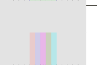
(A) (B)

Figure A.1: (A) The site ${s}_{j}$ is isolated. (B) The overlay vertices of the cell $\partial K_{j}$ with the boundary of cells created later. Note the figure is vertically not to scale.

Let $\beta=10\left\lceil{\lg n}\right\rceil$, and let $\mathcal{E}$ be the event that in the first $\beta$ sites, there are sites that belong to both the top and bottom row. We have that $\rho=\mathop{\mathbf{Pr}}\!\left[{\bigl{.}\mathcal{E}}\right]=1-2\binom{n}{\beta}/\binom{2n}{\beta}\geq 1-2/n^{10}$, as $2^{\beta}\binom{n}{\beta}\leq\binom{2n}{\beta}$. The $j$th site ${s}_{j}$ (say it is located at $(x_{j},\Delta)$) is isolated, if none of the points $(x_{j}-\xi_{j},\pm\Delta),(x_{j}-\xi_{j}+1,\pm\Delta)\ldots,(x_{j}+\xi_{j},\pm\Delta)$ are present in the prefix ${T}_{j-1}=\left\langle{{s}_{1},\ldots,{s}_{j-1}}\right\rangle$, where $\xi_{j}=\left\lceil{n/8j}\right\rceil$. If a site ${s}_{j}$ is isolated, for $j\geq\beta$, then its cell is going to be U shaped (assuming $\mathcal{E}$ happened), “biting” a portion of the $x$-axis, as $\Delta\gg n$, see Figure A.1 (A).

The probability of the site ${s}_{j}$ inserted in the $j$th iteration to be isolated is at least a half, since the majority of the points not inserted yet are isolated. Indeed, consider a site $i$, for $i<j$, and consider the interval it “blocks” $Z_{i}=[x_{i}-\xi_{j},x_{i}+\xi_{j}]$ from being isolated. That is, if $x_{j}\in Z_{i}$, then ${s}_{j}$ is not isolated. The total number of integer numbers in the intervals $Z_{1},\ldots,Z_{j-1}$ is at most $\alpha_{j}=\left({2\xi_{j}+1}\right)(j-1)$, and as such the first $j-1$ sites, block at most $2\alpha_{j}$ sites (that are located either on the top or bottom row) from being isolated in the $j$th iteration. As such, we have

$$\mathop{\mathbf{Pr}}\!\left[{\Bigl{.}{s}_{j}\text{ is not isolated}}\right] \leq\frac{2\alpha_{j}}{2n-j}=\frac{2\left({2\xi_{j}+1}\right)(j-1)}{2n-j}\leq\frac{2\left({\bigl{.}2\left\lceil{n/8j}\right\rceil+1}\right)j}{2n-j}$$

$$\leq\frac{\left({n/2j+6}\right)j}{2n-j}\leq\frac{{n}/{2}+6j}{2n-j}\leq\frac{(1/2+6/20)n}{(2-1/20)n}=\frac{16}{39}\leq\frac{1}{2},$$

for $j\leq n/20$, and for $n$ sufficiently large.

If ${s}_{j}$ is indeed isolated (and we remind the reader that we assume it is located at $(x_{j},\Delta)$), then there are no other sites (at this stage) in the slab $[x_{j}-\xi_{j},x_{j}+\xi_{j}]\times[-\infty,+\infty]$. In particular, the interval $I_{j}=\big{[}x_{j}-\xi_{j}/2,x_{j}+\xi_{j}/2\big{]}$ that lies on the $x$-axis is in the interior of the Voronoi cell $K_{j}$ of ${s}_{j}$.

This implies that in the final overlay arrangement, $K_{j}$ intersects all the cells of the sites ${p}_{x_{j}-\xi_{j}/2}$, $\ldots,{p}_{x_{j}+\xi_{j}/2}$, as their cells intersect the interval $I_{j}$. This in turn implies that $\partial K_{j}$ contains at least $2\left\lfloor{\xi_{j}/2}\right\rfloor$ intersection with the boundaries of other cells in the final overlay, see Figure A.1 (B). This counts only “future” intersections of $\partial K_{j}$ with the boundaries of cells created later. In addition, a tiny perturbation in the locations of the sites, guarantees that the boundary of $K_{j}$, does not lie on the boundary of any other Voronoi cell being created in this process. As such, an overlay vertex is being counted only once by this argument.

We conclude that the expected complexity of the overlay is

$$\geq\mathop{\mathbf{Pr}}\!\left[{\bigl{.}\mathcal{E}}\right]\sum_{j=\beta+1}^{n/20}2\left\lfloor{\bigl{.}\xi_{j}/2}\right\rfloor\mathop{\mathbf{Pr}}\!\left[{\bigl{.}{s}_{j}\text{ is isolated}}\right]\geq\frac{1}{2}\cdot\frac{1}{2}\sum_{j=\beta+1}^{n/20}2\left\lfloor{\Bigl{.}\left\lceil{\bigl{.}n/8j}\right\rceil/2}\right\rfloor$$

$$\geq\frac{1}{2}\sum_{j=\beta+1}^{n/20}\left\lfloor{\Bigl{.}n/16j}\right\rfloor\geq\frac{n}{64}\sum_{j=\beta+1}^{n/20}\frac{1}{j}=\Omega\left({\bigl{.}n\log n}\right).$$

References

- [AE84] F. Aurenhammer and H. Edelsbrunner. An optimal algorithm for constructing the weighted voronoi diagram in the plane. Pattern Recognition, 17(2):251–257, 1984.
- [AHKS14] P. K. Agarwal, S. Har-Peled, H. Kaplan, and M. Sharir. Union of random minkowski sums and network vulnerability analysis. Discrete Comput. Geom., 52(3):551–582, 2014.
- [AKL13] F. Aurenhammer, R. Klein, and D.-T. Lee. Voronoi Diagrams and Delaunay Triangulations. World Scientific, 2013.
- [AKS13] P. K. Agarwal, H. Kaplan, and M. Sharir. Union of random minkowski sums and network vulnerability analysis. In Proc. 29th Annu. Sympos. Comput. Geom. (SoCG), pages 177–186, 2013.
- [Aur87] F. Aurenhammer. Power diagrams: Properties, algorithms and applications. SIAM J. Comput., 16(1):78–96, 1987.
- [Aur91] F. Aurenhammer. Voronoi diagrams: A survey of a fundamental geometric data structure. ACM Comput. Surv., 23:345–405, 1991.
- [CHR14] H.-C. Chang, S. Har-Peled, and B. Raichel. From proximity to utility: A Voronoi partition of Pareto optima. CoRR, abs/1404.3403, 2014.
- [CS89] K. L. Clarkson and P. W. Shor. Applications of random sampling in computational geometry, II. Discrete Comput. Geom., 4:387–421, 1989.
- [DHR12] A. Driemel, S. Har-Peled, and B. Raichel. On the expected complexity of Voronoi diagrams on terrains. In Proc. 28th Annu. Sympos. Comput. Geom. (SoCG), pages 101–110, 2012.
- [Dwy89] R. Dwyer. Higher-dimensional Voronoi diagrams in linear expected time. In Proc. 5th Annu. Sympos. Comput. Geom. (SoCG), pages 326–333, 1989.
- [Har98] S. Har-Peled. An output sensitive algorithm for discrete convex hulls. Comput. Geom. Theory Appl., 10:125–138, 1998.
- [Har11a] S. Har-Peled. Geometric Approximation Algorithms, volume 173 of Mathematical Surveys and Monographs. Amer. Math. Soc., 2011.
- [Har11b] S. Har-Peled. On the expected complexity of random convex hulls. CoRR, abs/1111.5340, 2011.
- [HR14] S. Har-Peled and B. Raichel. On the complexity of randomly weighted Voronoi diagrams. In Proc. 30th Annu. Sympos. Comput. Geom. (SoCG), pages 232–241, 2014.
- [Kle88] R. Klein. Abstract Voronoi diagrams and their applications. In Workshop on Computational Geometry, pages 148–157, 1988.
- [KLN09] R. Klein, E. Langetepe, and Z. Nilforoushan. Abstract Voronoi diagrams revisited. Comput. Geom., 42(9):885–902, 2009.
- [KRS11] H. Kaplan, E. Ramos, and M. Sharir. The overlay of minimization diagrams in a randomized incremental construction. Discrete Comput. Geom., 45(3):371–382, 2011.
- [Mul94] K. Mulmuley. Computational Geometry: An Introduction Through Randomized Algorithms. Prentice Hall, 1994.
- [OBSC00] A. Okabe, B. Boots, K. Sugihara, and S. N. Chiu. Spatial tessellations: Concepts and applications of Voronoi diagrams. Probability and Statistics. Wiley, 2nd edition edition, 2000.
- [Pet13] S. Pettie. Sharp bounds on davenport-schinzel sequences of every order. In Proc. 29th Annu. Sympos. Comput. Geom. (SoCG), SoCG ’13, pages 319–328, 2013.
- [Ray70] H. Raynaud. Sur l’enveloppe convex des nuages de points aleatoires dans . J. Appl. Probab., 7:35–48, 1970.
- [RS63] A. Rényi and R. Sulanke. Über die konvexe Hülle von zufällig gerwähten Punkten I. Z. Wahrsch. Verw. Gebiete, 2:75–84, 1963.
- [SA95] M. Sharir and P. K. Agarwal. Davenport-Schinzel Sequences and Their Geometric Applications. Cambridge University Press, New York, 1995.
- [San53] L. Santalo. Introduction to Integral Geometry. Paris, Hermann, 1953.
- [Sha94] M. Sharir. Almost tight upper bounds for lower envelopes in higher dimensions. Discrete Comput. Geom., 12:327–345, 1994.
- [SW93] R. Schneider and J. A. Wieacker. Integral geometry. In P. M. Gruber and J. M. Wills, editors, Handbook of Convex Geometry, volume B, chapter 5.1, pages 1349–1390. North-Holland, 1993.
- [WW93] W. Weil and J. A. Wieacker. Stochastic geometry. In P. M. Gruber and J. M. Wills, editors, Handbook of Convex Geometry, volume B, chapter 5.2, pages 1393–1438. North-Holland, 1993.