Self-force via Green functions and worldline integration

Abstract

A compact object moving in curved spacetime interacts with its own gravitational field. This leads to both dissipative and conservative corrections to the motion, which can be interpreted as a self-force acting on the object. The original formalism describing this self-force relied heavily on the Green function of the linear differential operator that governs gravitational perturbations. However, because the global calculation of Green functions in non-trivial black hole spacetimes has been an open problem until recently, alternative methods were established to calculate self-force effects using sophisticated regularization techniques that avoid the computation of the global Green function. We present a method for calculating the self-force that employs the global Green function and is therefore closely modeled after the original self-force expressions. Our quantitative method involves two stages: (i) numerical approximation of the retarded Green function in the background spacetime; (ii) evaluation of convolution integrals along the worldline of the object. This novel approach can be used along arbitrary worldlines, including those currently inaccessible to more established computational techniques. Furthermore, it yields geometrical insight into the contributions to self-interaction from curved geometry (back-scattering) and trapping of null geodesics. We demonstrate the method on the motion of a scalar charge in Schwarzschild spacetime. This toy model retains the physical history-dependence of the self-force but avoids gauge issues and allows us to focus on basic principles. We compute the self-field and self-force for many worldlines including accelerated circular orbits, eccentric orbits at the separatrix, and radial infall. This method, closely modeled after the original formalism, provides a promising complementary approach to the self-force problem.

I Introduction

Gravitational waves emitted by binary systems featuring black holes contain a wealth of information about gravity in the strong field regime. Of particular interest is the case of a compact body of mass $m$ (e.g. a neutron star or black hole) in orbit around a larger black hole of mass $M$, such that $m/M\ll 1$. In this scenario, the radiation reaction timescale is much longer than the orbital period, and the system undergoes many cycles in the vicinity of the innermost stable circular orbit (typically, $\sim M/m$ in the final year before coalescence). The gravitational wave signal provides a direct probe of the spacetime of the massive black hole.

In the self-force interpretation, the compact body’s motion is associated with a worldline defined on the background spacetime of the larger partner. In the test-body limit $m=0$, that worldline is a geodesic of the background. For a finite mass, the worldline is accelerated by a gravitational self-force as the compact body interacts with its own gravitational field. The self-force has a dissipative and a conservative part, which drive an inspiraling worldline.

The calculation of the self-force in gravitational physics is an important problem from both a fundamental and an astrophysical point of view (see reviews Barack (2009); Poisson et al. (2011)). Fundamentally, knowing the gravitational self-force gives insight into the basic physical processes that determine the motion of a compact object in a curved background spacetime. This problem has its roots in the motion of an electrically-charged particle in flat spacetime Dirac (1938), though the physics of the gravitational self-force and electromagnetic radiation reaction are quite different. Astrophysically, the gravitational self-force is important because it drives the inspiral of a binary with an extremely small mass ratio ($\sim 10^{-5}$–$10^{-7}$). Such systems are expected gravitational wave sources for space-based detectors (e.g., eLISA Amaro-Seoane et al. (2012a, b)) that will provide detailed information about the evolution of galactic mergers, general relativity in the strong-field regime, and possibly the nature of dark energy, among others yel .

An expression for the gravitational self-force was formulated first in 1997 by Mino, Sasaki & Tanaka Mino et al. (1997) and Quinn & Wald Quinn and Wald (1997). Working independently, they obtained the MiSaTaQuWa (pronounced Mee-sah-tah-kwa) equation: an expression for the self-force at first-order in the mass ratio (in recent years, a more rigorous foundation for this formula has been established Gralla and Wald (2008); Pound (2010a, b) and second-order extensions in $m/M$ have been proposed Detweiler (2012); Pound (2012a); Gralla (2012); Pound (2012b)). The MiSaTaQuWa force can be split into “instantaneous” and “history-dependent” terms,

$$F^{\alpha}=F^{\alpha}_{\text{inst}}+F^{\alpha}_{\text{hist}}.$$ (1)

The instantaneous terms encapsulate the interaction between the source and the local spacetime geometry, and appear at a higher than leading order in the mass ratio. The history-dependent term involves the worldline integration of the gradient of the retarded Green function, which indicates a dependence on the past history of the source’s motion. The integral extends to the infinite past and is truncated just before coincidence at $\tau-\tau^{\prime}=\epsilon\rightarrow 0^{+}$. The dependence on the history of the source is due to gravitational perturbations that were emitted in the past by the source.

Describing and understanding gravitational self-force effects is complicated due to the gauge freedom and the computational burdens from the tensorial structure of gravitational perturbations. An important stepping stone for computing gravitational self-force has historically been scalar models. These models avoid the technical complications of the gravitational problem but still capture some essential features of self-force, in particular, the history-dependence.

The retarded Green function (RGF) for the scalar field is defined as the fundamental solution $G_{\rm ret}(x,x^{\prime})$ which yields causal solutions of the inhomogeneous scalar wave equation

$$\Box_{x}\Phi(x)=-4\pi\rho(x)$$ (2)

through

$$\Phi(x)=\int G_{\rm ret}(x,x^{\prime})\rho(x^{\prime})\sqrt{-g(x^{\prime})}\,d^{4}x^{\prime}.$$ (3)

Here, $G_{\rm ret}(x,x^{\prime})$ is a distribution which acts on test functions $\rho(x^{\prime})$ and also depends on the field point $x$, with the property that its support is $x^{\prime}\in J^{-}(x)$, where $J^{-}(x)$ is the causal past of $x$. This can be expressed as

$$\Box_{x}G_{\rm ret}(x,x^{\prime})=-4\pi\delta_{4}(x,x^{\prime})\,,$$ (4)

along with appropriate boundary conditions. Here, $\delta_{4}(x,x^{\prime})=\delta_{4}(x-x^{\prime})/\sqrt{-g}$ is the four-dimensional invariant Dirac delta distribution and $g$ is the determinant of the metric $g_{\mu\nu}$.

It was shown by Quinn Quinn (2000) that the self-field of a particle with scalar charge $q$ depends on the past history of the particle’s motion through

$$\Phi_{\rm hist}(z^{\lambda})={} q\lim_{\epsilon\to 0^{+}}\int_{-\infty}^{\tau-\epsilon}G_{\rm ret}(z^{\lambda},z^{\lambda^{\prime}})\,d\tau^{\prime}\,.$$ (5)

Here, $z^{\lambda}(\tau)$ describes the particle’s worldline parameterized by proper time $\tau$ and a prime on an index means that it is associated with the worldline parameter value $\tau^{\prime}$ (e.g., $z^{\alpha^{\prime}}=z^{\alpha}(\tau^{\prime})$). Likewise, Quinn showed that the self-force experienced by the particle can be written as $F^{\alpha}=F^{\alpha}_{\text{inst}}+F^{\alpha}_{\text{hist}}$ where $F^{\alpha}_{\text{inst}}$ is the “instantaneous” force, which vanishes for geodesic motion in a vacuum spacetime. The history-dependent term is

$$F^{\alpha}_{\text{hist}}(z^{\lambda})=q^{2}g^{\alpha\beta}\lim_{\epsilon\rightarrow 0^{+}}\int_{-\infty}^{\tau-\epsilon}\nabla_{\beta}G_{\rm ret}(z^{\lambda},z^{\lambda^{\prime}})\,d\tau^{\prime}.$$ (6)

The covariant derivative is taken with respect to the first argument of the RGF. The main difficulty in computing the self-field and the self-force through (5) and (6), respectively, is the computation of the RGF along the entire past worldline of the particle.

In addition to its role in computing the self-force the Green function also plays an essential part in understanding wave propagation. When the Green function to a linear partial differential operator, such as the wave operator, is known, any concrete solution with arbitrary initial data and source can be constructed via a simple convolution. Naturally, much effort has been devoted to the study and the calculation of Green functions in curved spacetimes, but a sufficiently accurate, quantitative description of its global behavior has remained an open problem until recently.

There are various difficulties regarding the calculation of Green functions in curved spacetimes. In four dimensional flat spacetime the RGF is supported on the lightcone only (when the field is massless), whereas in curved spacetimes the RGF has extended support also within the lightcone (here “lightcone” refers to the set of points $x$ connected to $x^{\prime}$ via null geodesics). Further, the lightcone generically self-intersects along caustics due to focusing caused by spacetime curvature.

These rich features of the RGF make it difficult to compute globally. A local approximation is not sufficient to evaluate the integral in (6) because the amplitude at a point on the worldline depends on the entire past history of the source. Early attempts Anderson and Hu (2004); Anderson et al. (2005, 2006); Ottewill and Wardell (2008, 2009) were founded upon the Hadamard parametrix Hadamard (1923), which gives the RGF in the form

$$G_{\rm ret}(x,x^{\prime})=\Theta_{-}(x,x^{\prime})\big{[}U(x,x^{\prime})\delta(\sigma)-V(x,x^{\prime})\Theta(-\sigma)\big{]}.$$ (7)

Here $U$ and $V$ are smooth biscalars, $\Theta(\cdot)$ is the Heaviside function, $\Theta_{-}(x,x^{\prime})$ is unity when $x^{\prime}$ is in the past of $x$ (and zero otherwise), and $\sigma=\sigma(x,x^{\prime})$ is the Synge world-function (i.e., one-half of the squared distance along the geodesic connecting $x$ and $x^{\prime}$). The Hadamard parametrix is only valid in the region in which $x$ and $x^{\prime}$ are connected by a unique geodesic (more precisely, if $x$ lies within a causal domain, commonly referred to using the less precise term normal neighborhood, of $x^{\prime}$ Friedlander (1975)). In strongly curved spacetimes the contribution from outside the normal neighbourhood cannot be neglected. Therefore, the Hadamard parametrix is insufficient for computing worldline convolutions. A method of matched expansions was outlined Poisson and Wiseman (1998); Anderson and Wiseman (2005), in which a quasi-local expansion for $G_{\rm ret}$, based on the Hadamard parametrix, would be matched onto a complementary expansion valid in the more distant past.

Despite initial promise, this idea for the global evaluation of the RGF proved difficult to implement, and other schemes for computing self-force came to prominence: the mode-sum regularization method Barack and Ori (2000) and the effective source method Vega and Detweiler (2008); Barack and Golbourn (2007). A practical advantage of these methods is that they work at the level of the (sourced) field rather than requiring global knowledge of RGFs. These methods require a regularization procedure based on a local analysis of the Green function by a decomposition into the singular and regular fields given by Detweiler & Whiting Detweiler and Whiting (2003). They have yielded impressive results Burko (2000a, b); Burko et al. (2001); Barack and Burko (2000); Detweiler et al. (2003); Diaz-Rivera et al. (2004); Vega et al. (2009); Haas (2007); Burko and Liu (2001); Warburton and Barack (2010, 2011); Keidl et al. (2007); Barack and Lousto (2002); Barack and Sago (2007); Detweiler (2008); Barack and Sago (2009); Shah et al. (2011); Canizares et al. (2010); Keidl et al. (2010); Dolan and Barack (2011); Haas (2011); Dolan et al. (2011); Barack and Sago (2011); Shah et al. (2012); Dolan and Barack (2013); Dolan et al. (2013), including the computation of self-consistent orbits at first-order in the mass ratio Warburton et al. (2012); Diener et al. (2012); Lackeos and Burko (2012). See Barack (2009) for a recent review of numerical self-force computations.

The steady progress in the computation of the self-force compared with the lack of quantitative results on global Green functions may have led to the notion that the computation of the self-force via the integration of the RGF was not practicable. Nevertheless, there has been recent work toward the global calculation of the RGF. The method of matched expansions for history-integral evaluation was revisited in Casals et al. (2009a), where it was shown that a distant-past expansion for the GF could be used to compute the self-force in the Nariai spacetime (a black hole toy model). Subsequently, steps were taken towards overcoming the technical difficulties with applying the analysis on realistic black-hole spacetimes Dolan and Ottewill (2011); Casals and Ottewill (2013, 2012).

An interesting by-product of these investigations has been an improved understanding of the structure of the RGF in spacetimes with caustics. While it was already known (e.g., Garabedian (1998); Ikawa (2000)) that singularities in the global RGF occur when the two spacetime points are connected via a null geodesic, the specific form of the singularities beyond the normal neighborhood was not previously known within general relativity. Ori Ori noted that the singular part of the RGF undergoes a transition each time the wavefront encounters a caustic, typically cycling through a four-fold sequence $\delta(\sigma)\rightarrow 1/(\pi\sigma)\rightarrow-\delta(\sigma)\rightarrow-1/(\pi\sigma)\rightarrow\delta(\sigma)$ (there are some exceptions to this four-fold cycle). Such four-fold structure can be understood as the wavefront picking up a phase $-\pi/2$ every time it crosses a caustic Casals et al. (2009a). In fact, this property has first been discovered in optics in the late 19th century Gouy (1890) and is related to the so-called Maslov index Maslov (1972, 1965). The phase transitions were confirmed via analytic methods on Schwarzschild spacetime Dolan and Ottewill (2011) and black hole toy model space times Casals et al. (2009a); Casals and Nolan (2012). A general mathematical analysis of the effect of caustics on wave propagation in general relativity was given in Harte and Drivas (2012).

Two recent developments along this line of research play an essential role for this paper. The first one is the numerical approximation of the global Green function in Schwarzschild spacetime Zenginoglu and Galley (2012). By replacing the delta-distribution source in (4) by a narrow Gaussian and evolving the scalar wave equation numerically, it was possible to provide the first global approximation of the RGF Zenginoglu and Galley (2012). The source in (4) generates “echoes” of itself due to trapping at the photon sphere, which were called “caustic echoes” in Zenginoglu and Galley (2012). An ideal observer at null infinity first measures the direct signal from the delta-distribution source, and later encounters, at nearly regular time intervals, exponentially-decaying caustic echoes. Both the arrival intervals and the exponential decay are determined by the properties of null geodesics around the photon sphere (their travel time and Lyapunov exponent). This work also provided a physical understanding of the four-fold sequence in caustic echoes: the trapping causes the wavefront to intersect itself at caustics as encapsulated by a Hilbert transform Zenginoglu and Galley (2012), which is equivalent to the $-\pi/2$ phase shift observed previously. A two-fold cycle was also observed and explained in Zenginoglu and Galley (2012); Casals and Nolan (2012) whenever the field point was in the equatorial plane (with the source) at an azimuthal angle of $\varphi=n\pi$ for $n$ an integer. Eventually, the echoes diminish below the late-time tail.

The second development is the culmination of previous semi-analytical efforts Casals et al. (2009a); Dolan and Ottewill (2011); Casals and Ottewill (2013, 2012) in the calculation of the global RGF in Schwarzschild spacetime using the method of matched expansions Casals et al. (2013). The RGF was calculated semi-analytically in the more distant past using a Fourier-mode decomposition and contour-deformation in the complex frequency plane, which also allowed for the computation of the self-force on a scalar charge in Schwarzschild spacetime.

In this paper, we combine a numerically computed global approximation to the RGF based on Zenginoglu and Galley (2012) with semi-analytic approximations at early and late times Casals et al. (2013) to compute the self-force for arbitrary motion via the worldline convolution integral, Eq. (6). To demonstrate the basic principles, we focus on the self-force on a scalar charge in a Schwarzschild background spacetime.

Our calculations consist of two parts. First, we construct quantitative global approximations of the Green function in Schwarzschild spacetime by replacing the delta-distribution by a narrow Gaussian Zenginoglu and Galley (2012). We augment the numerical calculation with analytical approximations through quasi-local expansions at early times (Ottewill and Wardell (2008); Wardell (2009); Casals et al. (2009b)) and through branch-cut integrals at late times Casals and Ottewill (2012, 2014). Second, we directly evaluate the convolution integrals for the self-field (5) and the self-force (6) at the desired point along the given worldline. We discuss a variety of orbital configurations, including accelerated circular orbits, eccentric geodesic orbits on the separatrix, and radial infall.

Beyond its direct relation to the original formalism, there are two additional motivations for computing the self-force through worldline convolutions of the Green function. The first motivation is conceptual: the method allows us to answer questions such as, how does the self-force depend on the past-history, and how far back in the history must one integrate to obtain an accurate estimate of the convolution. The second motivation is complementarity: the method is well-suited to computing the self-force along aperiodic (or nearly aperiodic) trajectories, such as unbound orbits, highly-eccentric or zoom-whirl orbits, and ultra-relativistic trajectories. These motions are difficult for or inaccessible to existing methods.

We believe this work challenges a perception that the original formulation by MiSaTaQuWa is ill-suited to practical calculations. We aim to demonstrate that the new method has the potential to make self-force calculations via worldline convolutions of Green functions as routine and as accurate as (time-domain) computations via the more established methods of mode-sum regularization and effective source.

In Sec. II we describe methods for constructing the RGF with numerical (II.1) and semi-analytic (II.2) approaches. In Sec. III we validate our method (III.1) and present a selection of results for three examples of motion: accelerated circular orbits (III.2), eccentric geodesics (III.3), and radial infall (III.4). We conclude with a discussion in Sec. IV. Throughout we choose conventions with $G=c=1$ and metric signature $(-+++)$.

II Construction of the RGF

The most difficult technical step in our computation of self-force is the construction of the global RGF. In Sec. II.1 we approximate the Green function numerically by replacing the delta-distribution by a narrow Gaussian in the initial data using the Kirchhoff formalism. We exploit the spherical symmetry of the background by performing a spherical harmonic decomposition and solving (1+1) dimensional wave equations for the Green function using standard numerical methods along with double hyperboloidal layers. In Sec. II.2 we augment the numerical solution at early and late times with semi-analytic approximations based on the quasi-local expansion and late-time behavior.

II.1 Numerical computation of the RGF

The global construction of the RGF in Zenginoglu and Galley (2012) used a narrow Gaussian to approximate the 4-dimensional Dirac delta-distribution source in (4) as,

$$\delta_{4}(x-x^{\prime})\approx\frac{1}{(2\pi\bar{\varepsilon}^{2})^{2}}\exp\!\left[-\sum_{\alpha=0}^{3}\frac{(x^{\alpha}-x^{\prime}{}^{\alpha})^{2}}{2\bar{\varepsilon}^{2}}\right].$$ (8)

Here, $\bar{\varepsilon}$ is the width of the Gaussian centered at the base point $x^{\prime}$. The numerical construction in Zenginoglu and Galley (2012) is performed in (3+1) dimensions and does not rely on (or exploit) any symmetries. In this paper we use the Gaussian approximation not in the source but in initial data. We use a Kirchhoff representation of the solution of the initial value problem corresponding to a given Cauchy surface in terms of the RGF and then set Gaussian initial data to recover an approximation to the RGF. The Kirchhoff representation can also be used in (3+1)-dimensions. However, in a subsequent step we perform an $\ell$-mode decomposition to exploit the spherical symmetry of the background, and reduce the wave equation to (1+1) dimensions, rather than (3+1) dimensions.

To summarize, our approach differs from Zenginoglu and Galley (2012) in the dimensionality of the time-domain wave equation [(1+1)- versus (3+1)-dimensions] and in the role of the approximated delta-distribution: as a source to the wave equation in Zenginoglu and Galley (2012) and as initial data in our approach.

II.1.1 RGF from impulsive initial data

Given Cauchy data on a spatial hypersurface $\Sigma$, the Kirchhoff representation in terms of the RGF can be used to determine the solution of the homogeneous wave equation,

$$\Box\Psi=0$$ (9)

at an arbitrary point $x^{\prime}$ in the past of $\Sigma$,

$$\Psi(x^{\prime})={} -\frac{1}{4\pi}\int_{\Sigma}\big{[}G_{\rm ret}(x,x^{\prime})\nabla^{\mu}\Psi(x)$$

$${\hskip 56.0088pt}-\Psi(x)\nabla^{\mu}G_{\rm ret}(x,x^{\prime})\big{]}d\Sigma_{\mu}.$$ (10)

Here, $d\Sigma_{\mu}=n_{\mu}\sqrt{h}\,d^{3}\mathbf{x}$ is the future-directed surface element on $\Sigma$, where $n_{\mu}=-\alpha\delta_{\mu}^{0}$ is the future-directed unit normal to the surface, $\alpha$ is the lapse, and $h$ is the determinant of the induced metric. Using reciprocity, there is also an equivalent representation in terms of the advanced Green function but we are interested in the RGF in this paper.

We choose a time coordinate $t$ (not necessarily Schwarzschild time) so that the surface $\Sigma$ corresponds to $t=t_{0}$. Setting initial data

$$\Psi(x)|_{\Sigma}=\Psi(t_{0},\mathbf{x})=0$$ (11a)

$$n_{\mu}\nabla^{\mu}\Psi(x)|_{\Sigma}=n_{\mu}\nabla^{\mu}\Psi(t_{0},\mathbf{x})=-4\pi\delta_{3}\bigl{(}\mathbf{x},\mathbf{x}_{0}\bigr{)}\,,$$ (11b)

Eq. (II.1.1) reduces to

$$\Psi(x^{\prime}) =\int_{\Sigma}G_{\rm ret}(t_{0},\mathbf{x};x^{\prime})\delta_{3}(\mathbf{x},\mathbf{x}_{0})\sqrt{h}\,d^{3}\mathbf{x}$$

$$=G_{\rm ret}(t_{0},\mathbf{x}_{0};x^{\prime}).$$ (12)

In other words, by evolving the homogeneous wave equation backwards in time with appropriate impulsive initial data, we obtain the RGF with the point $(t_{0},\mathbf{x}_{0})$ fixed on the hypersurface $\Sigma$ for all values of $x^{\prime}$ to the past. Thus, with just one calculation we obtain the RGF for fixed point $(t_{0},\mathbf{x}_{0})$ and all possible source points $z(\tau^{\prime})$ for trajectories passing through $(t_{0},\mathbf{x}_{0})$ appearing in the self-force history-integral. Note that we have been careful to describe this as fundamentally evolving backwards in time. The alternative—evolving Cauchy data forwards in time—would have instead yielded $G_{\rm ret}(x^{\prime};t_{0},\mathbf{x}_{0})$, which would be impractical for worldline convolutions as it would require a separate simulation for each point in the convolution integral. For time-reversal-invariant backgrounds such as the Schwarzschild spacetime the two procedures are, in fact, equivalent, but to emphasize the general applicability of the method we do not exploit that property here.

We can also compute derivatives of the Green function with respect to $x^{\prime}$ by simply differentiating the evolved field $\Psi(x^{\prime})$. However, in order to compute derivatives with respect to the source point $x$, as is demanded by a self-force calculation, it is necessary to modify the scheme by setting

$$\Psi(x)|_{\Sigma}=\Psi(t_{0},\mathbf{x})=0$$ (13a)

$$n_{\mu}\nabla^{\mu}\Psi(x)|_{\Sigma}=n_{\mu}\nabla^{\mu}\Psi(t_{0},\mathbf{x})=4\pi\partial_{i}\delta_{3}\bigl{(}\mathbf{x},\mathbf{x}_{0}\bigr{)}\,.$$ (13b)

Integrating by parts, we have

$$\Psi(x^{\prime}) =\int_{\Sigma}\partial_{i}G_{\rm ret}(t_{0},\mathbf{x};x^{\prime})\delta_{3}(\mathbf{x},\mathbf{x}_{0})\sqrt{h}\,d^{3}\mathbf{x}$$

$$=\partial_{i}G_{\rm ret}(t_{0},\mathbf{x}_{0};x^{\prime})\,,$$ (14)

and we obtain the spatial derivatives of the Green function, as required. Finally, for the time derivative we set

$$\Psi(x)|_{\Sigma}=\Psi(t_{0},\mathbf{x})=4\pi\delta_{3}\bigl{(}\mathbf{x},\mathbf{x}_{0}\bigr{)}$$ (15a)

$$n_{\mu}\nabla^{\mu}\Psi(x)|_{\Sigma}=n_{\mu}\nabla^{\mu}\Psi(t_{0},\mathbf{x})=0\,,$$ (15b)

to obtain

$$\Psi(x^{\prime}) =\int_{\Sigma}n_{\mu}\nabla^{\mu}G_{\rm ret}(t_{0},\mathbf{x};x^{\prime})\delta_{3}(\mathbf{x},\mathbf{x}_{0})\sqrt{h}\,d^{3}\mathbf{x}$$

$$=n_{\mu}\nabla^{\mu}G_{\rm ret}(t_{0},\mathbf{x}_{0};x^{\prime})\,.$$ (16)

II.1.2 Decomposition for 1+1 dimensions

In spherically symmetric spacetimes, we exploit the spherical symmetry of the background to develop an efficient scheme for solving (9) with initial data given by (11), (13), and (15). By decomposing the Green function into spherical harmonics and applying the Kirchhoff formula to the part depending on time and the radius, we significantly improve the efficiency of our calculations.

Consider the decomposition of the field into spherical harmonic $(\ell,m)$ modes,

$$\Psi(t,r,\theta,\varphi)=\sum_{\ell=0}^{\infty}\sum_{m=-\ell}^{\ell}\frac{1}{r}\Psi_{\ell m}(t,r)Y_{\ell m}(\vartheta,\varphi).$$ (17)

The spherical symmetry of the problem allows us to place the base point $x_{0}$ on the axis, in which case only the $m=0$ modes contribute. Then the spherical harmonic decomposition reduces to

$$\Psi(t,r,\gamma)=\sum_{\ell=0}^{\infty}\frac{1}{r}(2\ell+1)\Psi_{\ell}(t,r)P_{\ell}(\cos\gamma),$$ (18)

where $\Psi_{\ell}\equiv\Psi_{\ell m=0}$. Likewise, we decompose the Green function and its derivative by

$$G_{\rm ret}(t_{0},\mathbf{x}_{0};x^{\prime})=\frac{1}{r_{0}r^{\prime}}\sum_{\ell=0}^{\infty}(2\ell+1)G_{\ell}(t_{0},r_{0};t^{\prime},r^{\prime})P_{\ell}(\cos\gamma),$$ (19)

and

$$\partial_{r} G(t_{0},\mathbf{x}_{0};x^{\prime})=$$

$$\frac{1}{r^{\prime}}\sum_{\ell=0}^{\infty}(2\ell+1)P_{\ell}(\cos\gamma)\left\{\partial_{r}\left[\frac{1}{r}G_{\ell}(t_{0},r;t^{\prime},r^{\prime})\right]\right\}_{r=r_{0}}.$$ (20)

Choosing the standard Schwarzschild time $t$ and the tortoise coordinate $r^{\ast}\equiv r+2M\ln(r/2M-1)$, the Kirchhoff formula (II.1.1) reduces to

$$\Psi_{\ell}(t^{\prime},r^{\prime})=\int_{\Sigma}G_{\ell}(t,r;t^{\prime},r^{\prime})\partial_{t}\Psi_{\ell}(t,r)dr^{\ast}.$$ (21)

$$\Psi_{\ell}(t^{\prime},r^{\prime})={} \int_{-\infty}^{\infty}\big{[}G_{\ell}(t,r;t^{\prime},r^{\prime})\partial_{t}\Psi_{\ell}(t,r)$$

$${\hskip 56.0088pt}-\Psi_{\ell}(t,r)\partial_{t}G_{\ell}(t,r;t^{\prime},r^{\prime})\big{]}dr^{\ast}$$ (22)

Setting initial data

$$\Psi_{\ell}(t,r)|_{\Sigma}=0,\quad\partial_{t}\Psi_{\ell}(t,r)|_{\Sigma}=\delta(r^{\ast}-r^{\ast}_{0}),$$ (23)

yields

$$\Psi_{\ell}(t^{\prime},r^{\prime}) =\int_{-\infty}^{\infty}G_{\ell}(t_{0},r;t^{\prime},r^{\prime})\delta(r^{\ast}-r^{\ast}_{0})dr^{\ast}$$

$$=G_{\ell}(t_{0},r_{0};t^{\prime},r^{\prime}).$$ (24)

Thus, by evolving the homogeneous $1$+$1$ dimensional wave equation (see Eqs. (31) and (32) below) with this initial data, we obtain the $\ell$ modes of the retarded Green function with the retarded point $r_{0}$ fixed on the initial hypersurface. Similarly, we can compute the radial derivative of the Green function by choosing initial data

$$\Psi_{\ell}(t,r)|_{\Sigma}=0,\quad\partial_{t}\Psi_{\ell}(t,r)|_{\Sigma}=-\frac{f}{r}\partial_{r}\left[f^{-1}\delta(r^{\ast}-r^{\ast}_{0})\right]$$ (25)

with $f\equiv 1-2M/r$. This gives

$$\Psi_{\ell}(t^{\prime},r^{\prime}) =-\int_{-\infty}^{\infty}\frac{f}{r}G_{\ell}(t_{0},r;t^{\prime},r^{\prime})\partial_{r}\left[f^{-1}\delta(r^{\ast}-r^{\ast}_{0})\right]dr^{\ast}$$

$$=\partial_{r}\left[\frac{1}{r}G_{\ell}(t_{0},r;t^{\prime},r^{\prime})\right]_{r=r_{0}}.$$ (26)

Finally, to compute the $t$ derivative we set initial data

$$\Psi_{\ell}(t,r)|_{\Sigma}=\delta(r^{\ast}-r^{\ast}_{0}),\quad\partial_{t}\Psi_{\ell}(t,r)|_{\Sigma}=0,$$ (27)

which yields

$$\Psi_{\ell}(t^{\prime},r^{\prime}) =\int_{-\infty}^{\infty}\left[\partial_{t}G_{\ell}(t,r;t^{\prime},r^{\prime})\right]_{t=t_{0}}\delta(r^{\ast}-r^{\ast}_{0})dr^{\ast}$$

$$=\left[\partial_{t}G_{\ell}(t,r_{0};t^{\prime},r^{\prime})\right]_{t=t_{0}}.$$ (28)

We obtain $G_{\ell}$ and its $t$ and $r$ derivatives by solving the corresponding initial value problem. The $\gamma$ derivatives are trivially given by using (24) in (19) and differentiating the Legendre polynomials with respect to $\gamma$.

II.1.3 Gaussian approximation to the Dirac delta distribution and the smooth angular cutoff

We approximate the Dirac delta distribution in the initial data (see Eqs. (23), (25) and (27)) on our numerical grid by a Gaussian of finite width, $\varepsilon$. In the limit of zero width, the delta distribution is recovered,

$$\delta(r^{\ast}-r^{\ast}_{0})=\lim_{\varepsilon\to 0^{+}}\frac{1}{(2\pi\varepsilon^{2})^{1/2}}e^{-(r^{\ast}-r^{\ast}_{0})^{2}/2\varepsilon^{2}}$$ (29)

This replacement effectively limits the shortest length scales which can be represented by the spherical harmonic expansion of the field—in this way there is a direct correspondence between the use of a finite-width Gaussian and a finite number of $\ell$ modes. Higher $\ell$ modes oscillate more and more rapidly both in space and time. Once the scale of these oscillations becomes comparable to the width of the Gaussian, any higher $\ell$ modes are not faithfully resolved. The advantage of using a smooth Gaussian, however, is that this cutoff happens in a smooth fashion.

We cut off the formally infinite sum over $\ell$ in (19) and (II.1.2) at some finite $\ell_{\rm max}$. A sharp cutoff in a spectral expansion yields highly oscillatory, unphysical features in the result. The replacement of a delta distribution with a smooth Gaussian in our numerical scheme mitigates this somewhat; for a fixed Gaussian width $\varepsilon$ there exists a finite $\ell_{\rm max}$ which is sufficient to eliminate the unphysical oscillations (for a detailed discussion of the relation between $\varepsilon$ and $\ell_{\rm max}$ see Sec. IV A 3 of Casals et al. (2013)). However, for very small Gaussian widths this $\ell_{\rm max}$ may be unpractically large.

In this work, as previously in Casals et al. (2009a, 2013), we have employed a smooth sum method which is very effective in eliminating the high-frequency oscillations while maintaining the physically-relevant low $\ell$ contribution important for computing the self-force. The basic idea to to replace the sum in (18) (or, equivalently, in (19) and (II.1.2)) with a smooth cut off at large $\ell$ Hardy (1948),

$$\Psi(t,r,\gamma)=\sum_{\ell=0}^{\ell_{\rm max}}e^{-\ell^{2}/2\ell_{\rm cut}^{2}}\frac{1}{r}(2\ell+1)\Psi_{\ell}(t,r)P_{\ell}(\cos\gamma),$$ (30)

where we empirically choose $\ell_{\rm cut}=\ell_{\rm max}/5$. The introduction of such a smoothing factor can be related Casals et al. (2013) to: i) the “smearing” in the angular coordinate of the distributional features of the Green function, and ii) the replacement of the $\delta_{4}$-source in (4) by a “narrow” Gaussian distribution.

The effect of varying $\varepsilon$ and $\ell_{\rm cut}$ on the Green function can be seen in Fig. 1. The sharp features near caustic echoes are resolved only for small $\varepsilon$ and large $\ell_{\rm cut}$; but away from caustic echoes the Green function is well resolved even for large $\varepsilon$ and small $\ell_{\rm cut}$.

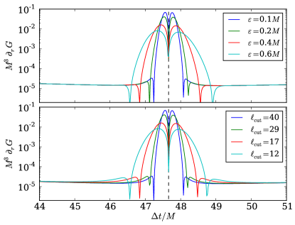
Figure 1: Top: The radial derivative of the Green function for the $e=0.5$, $p=7.2$ eccentric orbit case computed using Gaussians of varying widths and a fixed smooth-sum cutoff of $\ell_{\rm cut}=40$. As the width is decreased, the sharp features near the null geodesic crossing around $\Delta t\approx 47.6M$ are better resolved. Away from the null geodesic crossings, the improvement with decreasing width is much less significant. Bottom: Since a finite width Gaussian also implies an effective maximum number of $\ell$ modes, a very similar plot is obtained when the number of $\ell$ modes included is increased (with a fixed Gaussian width of $\varepsilon=0.1M$).

Because the regularized self-field is a smooth function of spacetime, the spectral representation in terms of spherical-harmonic modes converges exponentially with the number of $\ell$ modes and the small-$\ell$ modes seem sufficient. There are, however, some cases where this approximation is not very useful and large $\ell$ features become important. For example, for ultra-relativistic orbits close to the Schwarzschild light ring at $r=3M$, the exponentially-convergent regime is deferred to very large $\ell$ Akcay et al. (2012). In such cases, it is likely that alternative methods which capture the large-$\ell$ structure are more suitable, including asymptotic expansions of special functions Casals and Nolan (2012); Nolan (2013), WKB methods Dolan and Ottewill (2011), the geometrical optics approximation Zenginoglu and Galley (2012), and frozen Gaussian beams Lu and Yang (2011).

With our chosen numerical parameters, the dominant source of error in our calculation comes from two related issues: the fact that we only sum over a finite number of $\ell$ modes and that we use a Gaussian of finite width $\varepsilon$. Both approximations limit the minimum length scale (both in space and time) of the features that we can resolve. As shown in Fig. 2 the error from these approximations converges away quadratically in $\varepsilon$ and $1/\ell_{\rm cut}$. By repeating the calculation for a series of values of $\varepsilon$ and $\ell_{\rm max}$ one can extrapolate to $\varepsilon=0$ and $\ell_{\rm cut}=\infty$ using standard Richardson extrapolation.

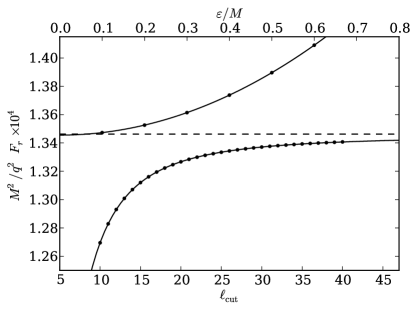
Figure 2: Extrapolation in $\ell_{\rm cut}$ (bottom curve) and $\varepsilon$ (top curve) when computing the radial component of the self-force for the $e=0.5$, $p=7.2$ eccentric orbit. The convergence in both cases is approximately quadratic, as indicated by the curves, which are a least squares fit of a quadratic function to the data. The dashed line indicates the high-accuracy value from Warburton and Barack (2011).

The fact that the extrapolation in both parameters can be done reliably allows for significant improvements in the accuracy of the numerical results. However, doing so requires multiple numerical simulations, one for each value of $\varepsilon$. Since the focus of this paper is not on achieving maximal accuracy but rather on demonstrating the feasibility of the method, we do not extrapolate in $\varepsilon$ for the results in Sec. III and instead rely on extrapolation in $\ell$ alone. Although this does not yield the same accuracy as additionally extrapolating in $\varepsilon$ (which gives an additional factor of 10 improvement in accuracy in our test cases), it does nevertheless improve the accuracy relative to the un-extrapolated result by a factor of 10.

II.1.4 Numerical evolution

For the Schwarzschild spacetime, it is convenient to choose coordinates that locally match the Regge-Wheeler form in the vicinity of the worldline, but which also map future null infinity and the future event horizon to finite values. This keeps the construction of initial data and the interpretation of results simple, while improving computational efficiency by eliminating problems with outer boundaries. To this end, we employ hyperboloidal compactification Zenginoglu (2008) in the form of a layer Zenginoglu (2011) with the standard Schwarzschild time and tortoise coordinates in the vicinity of the worldline and hyperboloidal coordinates far from the worldline using the double layer construction from Bernuzzi et al. (2012).

We choose a compactifying radial coordinate $\rho$ defined through $r_{\ast}=\rho/\Theta(\rho)$, where $\Theta$ is a function that is unity in a compact domain and smoothly approaches zero on both ends of the domain. The hyperboloidal time transformation is determined such that $t+r_{*}=\tau+\rho$ for $r_{\ast}\to-\infty$, and $t-r_{*}=\tau-\rho$ for $r_{\ast}\to\infty$, which implies that level sets of the new time coordinate $\tau$ are horizon-penetrating near the black hole and hyperboloidal near null infinity. See Bernuzzi et al. (2012) for details of this double hyperboloidal layer construction.

Substituting the spherical-harmonic decomposition of the field, Eq. (18), into the homogeneous wave equation, Eq. (9), we obtain $1$+$1$D equations for each of the $\Psi_{\ell}$ which can be written in first order in time form,

$$\partial_{\tau}\Psi_{\ell}= \frac{\Pi_{\ell}}{1\pm H}-\frac{H\partial_{\rho}\Psi_{\ell}}{1\pm H}\,,$$ (31)

$$\partial_{\tau}\Pi_{\ell}= \partial_{\rho}\Big{[}\frac{\partial_{\rho}\Psi_{\ell}}{1\pm H}-\frac{H\,\Pi_{l}}{1\pm H}\Big{]}$$

$$-(\Theta-\rho\,\Theta^{\prime})\Big{[}1-\frac{2M\Theta}{\rho}\Big{]}\Big{[}\frac{\ell(\ell+1)}{\rho^{2}}+\frac{2M\Theta}{\rho^{3}}\Big{]}\Psi_{\ell}\,,$$ (32)

where a prime denotes differentiation with respect to $\rho$, $\Pi_{\ell}\equiv(1\pm H)\partial_{\tau}\Psi_{\ell}+H\partial_{\rho}\Psi_{\ell}$, and the function $H$ is given by $H\equiv\pm\tfrac{d}{dr_{\ast}}(r_{\ast}-\rho)=\pm\left(1-\tfrac{\Theta^{2}}{\Theta-\rho\Theta^{\prime}}\right)$, where the undetermined signs are positive near null infinity and negative near the black hole Bernuzzi et al. (2012).

We evolve (31) and (32) for $200$ $\ell$ modes in the time domain using the method-of-lines formulation. We compute spatial derivatives using eighth-order accurate centered finite differencing. At the boundaries (corresponding to the black-hole horizon and null infinity) we use eighth-order asymmetric stencils without imposing any boundary conditions because all characteristics are purely outgoing in our hyperboloidal coordinates. We include a small amount of Kreiss-Oliger Kreiss and Oliger (1973) numerical dissipation to damp out high-frequency noise. We evolve forwards in time using standard fourth order Runge-Kutta time integration with a fixed step size equal to half of the spatial grid spacing. We use an equidistant spatial grid with a resolution of $\Delta r^{\ast}=0.01M$ in the Regge-Wheeler-Zerilli coordinate region. We choose a domain of $\rho\in[-150M,150M]$ with layer interfaces located at $\pm 135M$, so that all worldlines we consider are moving in the Regge-Wheeler-Zerilli coordinate region.

We set Gaussian initial data of width $\varepsilon=0.1M$. We evolve for a total time of $t=400M$, so that the remaining portion of the history integral has a negligible contribution to the self-force and its contribution to the self-field is well approximated by the late-time asymptotics described in Sec. II.2.2. We extract values on the worldlines by simultaneously evolving the equations of motion using the osculating orbits framework Pound and Poisson (2008) for the circular and eccentric orbits and using (42) for the radial infall case. We interpolate the values on the worldline using eighth order Legendre polynomial interpolation.

II.2 Analytical approximations to the retarded Green function

In this section we describe the two analytical approximations to the RGF, one valid at early times and one valid at late times, which we use as a substitute for the numerical solution in the regions where it cannot be used.

II.2.1 Quasi-local expansion

In the quasi-local region, the spacetime points $x$ and $x^{\prime}$ are assumed to be sufficiently close together that the RGF is uniquely given by the Hadamard parametrix, Eq. (7). The term involving $U(x,x^{\prime})$ does not contribute to the integrals in Eqs. (5) and (6) since, within those integrals, it has support only when $x=x^{\prime}$, and the integrals exclude this point. We will therefore only concern ourselves in the quasi-local region with the calculation of the function $V(x,x^{\prime})$.

The proximity of $x$ and $x^{\prime}$ implies that an expansion of $V(x,x^{\prime})$ in the separation of the points can give a good approximation within the quasi-local region. Reference Casals et al. (2009b) used a WKB method to derive such a coordinate expansion and gave estimates of its range of validity. Referring to the results therein, we have $V(x,x^{\prime})$ as a power series in $(t-t^{\prime})$, $(1-\cos\gamma)$, and $(r-r^{\prime})$,

$$V(x,x^{\prime})=\sum_{i,j,k=0}^{\infty}v_{ijk}(r)~{}(t-t^{\prime})^{2i}(1-\cos\gamma)^{j}(r-r^{\prime})^{k},$$ (33)

where $\gamma$ is the angular separation of the points and the $v_{ijk}$ are computable analytic functions of $r$. Up to an overall minus sign, Eq. (33) gives the quasi-local contribution to the RGF. It is straightforward to take partial derivatives of these expressions at either spacetime point to obtain the derivative of the Green function.

As proposed in Ref. Casals et al. (2009b), we use a Padé re-summation of Eq. (33) in order to increase the accuracy and extend the domain of validity of the quasi-local expansion. While not essential, this increases the region of overlap between the quasi-local and numerical Gaussian domains. Since Padé re-summation is only well defined for series expansions in a single variable, it is necessary to first expand $r^{\prime}$ and $\gamma$ in a Taylor series in $t-t^{\prime}$, using the equations of motion to determine the higher derivatives appearing in the series coefficients. Then, with $V(x,x^{\prime})$ written as a power series in $t-t^{\prime}$ alone, a standard diagonal Padé approximant of order $(t-t^{\prime})^{26}$ in both the numerator and denominator is constructed and used to represent the Green function in the quasi-local region.

II.2.2 Late-time behavior

It is known since the work of Price Price (1972a, b) that an initial field perturbation of a Schwarzschild black hole decays at late times with a leading power-law behavior: $t^{-2\ell-3}$ for the field mode with multipole $\ell$. This late-time behaviour is related to the form at large radius of the potential in the ordinary differential equation satisfied by the radial part of the perturbation, i.e., the Regge-Wheeler equation for general integer spin of the field. The form of the late-time tail can be derived from low-frequency asymptotics along the branch cut that the Fourier modes of the Green function possess in the complex-frequency plane Leaver (1986); Ching et al. (1995). In Casals and Ottewill (2012), the exact coefficients in the expansion at late times of the Green function modes at arbitrary radius were given up to the first four orders. In particular, a new behavior $t^{-2\ell-5}\log(t/M)$ was obtained in the third-order term, thus showing a deviation from a pure power-law expansion. In the present paper we have used the method presented in Casals and Ottewill (2012), which is described in detail in Casals and Ottewill (2014). This method is based on the ‘MST formalism’ Mano et al. (1996a, b); Sasaki and Tagoshi (2003). It consists of expressing the solutions to the radial ordinary differential equation as series of special functions, namely ordinary hypergeometric functions and confluent hypergeometric functions. These series have the advantage that they are particularly amenable to expansions for low frequency. We have used these series in order to obtain low-frequency asymptotic expansions up to next-to-leading order of the Green function modes along the branch cut. Finally, by integrating these expansions along the branch cut we obtain the late-time asymptotics of the full Green function, which we will to as the late-time tail.

III Results

In this section we present self-force computations for a variety of orbits at the point where the orbits pass through $r_{0}=6M$. One of the strengths of the Green function approach is that once the Green function and its derivatives are available, the self-force for all orbits passing through one point can be computed by simple worldline evaluations (see Fig. 3). The entire set of results in this section are obtained from just three numerical time-domain evolutions: for the Green function and its time and radial derivatives (because of the spherical-harmonic decomposition, angular derivatives act only on the Legendre polynomials and the numerical data required is the same as that for the undifferentiated Green function).

Figure 3: A sample of bound geodesic orbits having different eccentricities but passing through the same point $P$ at $r_{0}=6M$. For any of these geodesics, the history-dependent part of the self-field and self-force at $P$ can be computed from four numerical time-domain evolutions (i.e., $G$, $\partial_{t}G$, $\partial_{r}G$, and $\partial_{\varphi}G$) with $P$ as the base point. The same is true for any worldline passing through $P$, even accelerated or unbound ones.

Here, we focus on three particular families which best demonstrate the flexibility of the method:

• Accelerated circular orbits, including ultra-relativistic and static limits.

• Geodesic eccentric orbits, including those near the separatrix between stable and unstable bound geodesics.

• Radial infall, reflecting the ability to handle unbound motion.

Before discussing these cases, we first validate our methods and establish the accuracy of our results by comparing against two cases for which accurate self-force values are available.

III.1 Validation against existing results

The frequency-domain based mode-sum regularization method is unparalleled in its ability to compute highly accurate values for the self-force in cases where the retarded field is given by a discrete spectrum involving a small number of Fourier modes Haas and Poisson (2006); Detweiler et al. (2003); Warburton and Barack (2011); Heffernan et al. (2012). Here, we consider two cases which were computed to high accuracy using the methods in Warburton and Barack (2011); Heffernan et al. (2012) and which were considered in Casals et al. (2013): a circular geodesic orbit of radius $r_{0}=6M$, and an eccentric orbit with eccentricity $e=0.5$ and semilatus rectum $p=7.2$.

Our numerical calculations employ a number of approximations:

• Numerical discretization of the $1$+$1$ dimension equation. This introduces a numerical error which arises from errors in the time integration, spatial finite differencing, and interpolation of values to the worldline, all of which converge away with increasing resolution. Using our numerical grid with spacing $\Delta r^{\ast}=0.01$M, these errors are all negligible. For example, in the most difficult case of the radial component of the self-force for the eccentric orbit, a higher resolution simulation with $\Delta r^{\ast}=0.005$M was used to estimate that the relative error from numerical discretization is $\sim 1\times 10^{-5}$.

• Taylor series approximation at early times. The accuracy of the Taylor series approximation decreases as the field and source points are separated. By repeating the calculation for a range of matching times (between the Taylor series and the numerical solution) in the region $t_{m}\in[15M,21M]$, we obtained relative differences in the radial self-force for the eccentric case of $\sim 10^{-3}$. Although these differences are comparable to those arising from a finite cut-off in the sum over $\ell$, it turns out that this is because the two issues are closely linked: by using a larger cutoff in the $\ell$-sum, the errors from matching are also reduced. This connection also allows us to use the error from the finite cut-off in the $\ell$-sum as an accurate approximation for the error from matching by choosing the matching time so that the error is no larger than that from the $\ell$-sum.

• Asymptotic expansions for the late-time tail. These expansions become increasingly unreliable as field and source points are brought closer together. By numerically evolving to $t=400M$, we make sure that the remainder of the history-integral contributes a negligible amount to the self-force. In our test eccentric orbit case, the relative contribution is $\sim 5\times 10^{-5}$.
  The contribution to the history integral from late times is more significant for the scalar field because the Green function decays more slowly in time than its derivative. However, even in this case the magnitude of the late-time tail history integral for the circular orbit is only $\sim 10^{-5}$ (compared to $\sim 10^{-2}$ for the entire history integral) and any error in our approximation is considerably smaller. We may therefore neglect errors from the late-time portion of the history integral. Unfortunately, this does not hold for generic orbits. For example, for the eccentric orbit test case, the late-time-tail-integral error slightly dominates over other sources of error in the calculation; this dominance becomes more and more pronounced for orbits whose radial position varies more and more unpredictably with time. For this reason, when quoting errors for the self-field, we use the magnitude of the late-time tail integral as an estimate under the assumption that it always provides an upper-bound (if somewhat over-conservative) approximation.

• Replacement of a delta distribution with a Gaussian. This causes both a spurious pulse at early times and a smoothing out of any sharp features. The initial pulse is eliminated by replacing the Green function at early times with its quasilocal Taylor series expansion. With our chosen Gaussian width of $\varepsilon=0.1M$, the relative error caused by the finite-width Gaussian is $\sim 1\times 10^{-3}$ (see Fig. 2).

• Cutting off the infinite sum over $\ell$. Like the finite width Gaussian, this has the effect of smoothing out of any sharp features. We estimate this error by the difference between the self-force computed using $\ell_{\rm cut}=40$ and the value obtained by extrapolating the curve in Fig. 2, which gives a relative error $\sim 4\times 10^{-3}$.

In our test cases, the dominant source of error therefore comes from the choice of $\varepsilon$ and the cutoff in the sum over $\ell$. Because the two sources of error are intimately connected (a choice of $\varepsilon$ results in an effective maximum $\ell$ which can be resolved) we estimate the error in our results by considering the errors in the sum over $\ell$ (for sufficiently small $\varepsilon$). This estimate is conservative because it ignores accuracy improvements from extrapolating in $\ell_{\rm cut}$. The true accuracy of the computed self-force is up to an order of magnitude better (see Table 1).

		Computed value	Rel. Err.	Est. Err.
Circular	$M/q\,\Phi$	$-5.45517\times 10^{-3}$	$6\times 10^{-5}$	$3\times 10^{-3}$
	$M^{2}/q^{2}\,F_{t}$	$3.60779\times 10^{-4}$	$4\times 10^{-4}$	$2\times 10^{-3}$
	$M^{2}/q^{2}\,F_{r}$	$1.67861\times 10^{-4}$	$8\times 10^{-4}$	$2\times 10^{-3}$
	$M^{2}/q^{2}\,F_{\varphi}$	$-5.30452\times 10^{-3}$	$5\times 10^{-5}$	$5\times 10^{-4}$
Eccentric	$M/q\,\Phi$	$-7.70939\times 10^{-3}$	$1\times 10^{-3}$	$1\times 10^{-3}$
	$M^{2}/q^{2}\,F_{t}$	$6.65241\times 10^{-4}$	$2\times 10^{-4}$	$1\times 10^{-3}$
	$M^{2}/q^{2}\,F_{r}$	$1.3473\times 10^{-4}$	$8\times 10^{-4}$	$4\times 10^{-3}$
	$M^{2}/q^{2}\,F_{\varphi}$	$-7.28088\times 10^{-3}$	$4\times 10^{-5}$	$5\times 10^{-4}$

Table 1: Numerical results for circular and eccentric orbit test cases, including estimated errors.

In Table 1 we compare the results of our numerical Green-function calculation with reference values computed using the frequency-domain mode-sum regularization method. We also give internal error estimates based on the assumption that the choice of a finite $\ell_{\rm cut}$ reasonably reflects the dominant source of error in the self-force and the finite integration time is the dominant source of error in the self-field. Our goal here is not to show that the Green function method improves on the accuracy of existing methods. Frequency-domain based methods are the accuracy leaders for cases where they can be used. But the Green function method provides a highly flexible and complementary approach which gives good results using modest computational resources. Furthermore, it would not be difficult to significantly improve on the accuracy of the results presented here through either brute force methods (higher resolution, more $\ell$ modes, smaller Gaussian, higher order Taylor series and longer integration times) or through readily available improvements to the numerics (better hyperboloidal coordinates, spectral methods for spatial derivatives, improved time-integration schemes and analytic asymptotics for the large-$\ell$ modes Nolan (2013); Casals and Nolan (2012)). We leave the implementation of such improvements for future work.

III.2 Accelerated circular orbits

We consider a particle in a circular orbit of radius $r_{0}$ and constant angular velocity $\Omega$, so that the azimuthal angle coordinate is given by $\varphi=\Omega\,t$. For such orbits, the redshift factor is

$$z\equiv\frac{1}{u^{t}}=\sqrt{1-\frac{2M}{r_{0}}-r_{0}^{2}\Omega^{2}}.$$ (34)

The three special cases $\Omega^{2}=\{0,M/r_{0}^{3},(r_{0}-2M)/r_{0}^{3}\}$ correspond to a static particle, circular geodesic, and null orbit, respectively. Because the orbit is accelerated, there is an additional instantaneous contribution to the self-force not present for a geodesic. This instantaneous contribution is given by Quinn and Wald (1997)

$$F^{\rm inst}_{\mu}=\frac{q^{2}}{3}(g_{\mu}{}^{\nu}+u_{\mu}u^{\nu})\frac{Da_{\nu}}{d\tau}\,,$$ (35)

which, in the constantly accelerated circular orbit case, has components

$$F^{\rm inst}_{t}=\frac{q^{2}M^{2}(r_{0}\!-\!2M)(n^{2}\!-\!1)}{3r_{0}^{5}z^{3}}\bigg{[}1\!+\!\frac{(r_{0}\!-\!2M)(n^{2}\!-\!1)}{r_{0}z^{2}}\bigg{]},$$

$$F^{\rm inst}_{r}=0,\quad F^{\rm inst}_{\theta}=0,$$

$$F^{\rm inst}_{\varphi}=-\frac{q^{2}M^{3/2}(r_{0}\!-\!2M)n(n^{2}\!-\!1)}{3r_{0}^{7/2}z^{3}}\bigg{[}1\!+\!\frac{M(n^{2}\!-\!1)}{r_{0}z^{2}}\bigg{]},$$ (36)

where $n\equiv\Omega/\Omega_{g}$, and $\Omega_{g}=(M/r_{0}^{3})^{-1/2}$ is the geodesic frequency.

We compute the RGF and its derivatives on all constantly accelerated circular orbits with radius $r_{0}=6M$, and plot the results in Fig. 4 as a function of the time $\Delta t/M$ from coincidence and of the orbital frequency $\Omega$ relative to the geodesic value. The figure shows the complex structure of the Green function that results from the interplay of wave propagation with the orbiting particle; the light shaded regions correspond to caustic echoes along the orbits. The dotted curves indicate the times at which a given circular orbit crosses a point with $\varphi=n\pi$ for $n$ a positive integer.

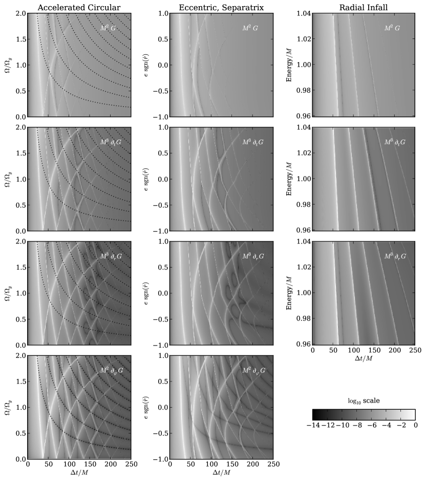
Figure 4: Plot of the Green function and its derivatives for all orbits considered in this paper, evaluated at the base point where the orbital radius is $r_{0}=6M$. The $x$-axis labels time $\Delta t/M$ from coincidence and the $y$-axis labels the parameter defining the orbit. The dotted curves for accelerated circular orbits correspond to the times at which the orbit crosses a point with an angle $\varphi=n\pi$, $n\in\mathbb{Z}^{+}$ relative to the Green function’s base point at $t=0$. Note: since light-shaded curves effectively correspond to null geodesics, the particular space-time points where two light-shaded curves intersect must necessarily lie, by symmetry, on a dotted curve (i.e., with $\varphi=n\pi$) and they are the caustic points which are encountered by the timelike orbits that we consider.

The left column in Fig. 4 shows the Green function itself (top left) and its derivatives (bottom three) evaluated along the orbits. As the shading in the plots indicate, the late-time tail decay is slowest for the Green function, faster for its time derivative, and fastest for the radial and azimuthal derivatives. We thus infer that late-time effects from back-scattering are more relevant for computing the self-field than they are for the self-force. This is in agreement with what was observed in Casals et al. (2013) in the specific instances of a circular geodesic and an eccentric orbit with $p=7.2$ and $e=0.5$. Conversely, caustic echoes give non-negligible contributions to the self-force at later times than they would for the self-field because the late-time tail contributes less. The contributions from the effects of curved geometry (back-scattering) and trapping (caustic echoes) to quantities of interest are clearer in our method than in other self-force calculation techniques.

The history-dependent part of the self-field and self-force evaluated along these orbits are given by

$$\Phi_{\rm hist}= q\sqrt{1-\frac{2M}{r_{0}}-r_{0}^{2}\Omega^{2}}\,\int^{0^{-}}_{-\infty}\!\!\!G_{\rm ret}(x;x^{\prime})dt^{\prime},$$

$$F^{\rm hist}_{\mu}= q^{2}\sqrt{1-\frac{2M}{r_{0}}-r_{0}^{2}\Omega^{2}}\,\int^{0^{-}}_{-\infty}\!\!\partial_{\mu}G_{\rm ret}(x;x^{\prime})dt^{\prime}.$$ (37)

These are plotted in the top panel of Fig. 5 as a function of $\Omega/\Omega_{g}$.

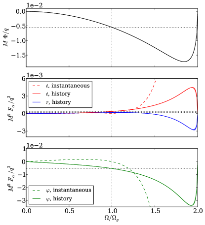
Figure 5: Regular part of the self-field and self-force on constantly accelerated circular orbits of radius $r_{0}=6M$ with different orbital frequencies $\Omega$ relative to the geodesic frequency $\Omega_{g}$. The motion is null when $\Omega=2\Omega_{g}$. The dashed black lines indicate the reference value of the self-field at the geodesic frequency from Haas and Poisson (2006). Error bars are included as shaded regions about the curves.

When the particle is at rest ($\Omega=0$) the self-field and self-force are consistent with zero within our error bars, as expected and in agreement with analytical results Wiseman (2000). Furthermore, the local and history-dependent pieces of the self-force components vanish separately, independently of each other. We also find that the history-dependent self-field and self-force vanish for a null circular orbit, [$\Omega=(r_{0}-2M)/r_{0}^{3}$]; this can be inferred immediately from Eq. (III.2) because the redshift factor,

$$z\big{|}_{\rm null~{}orbits}=\sqrt{1-\frac{2M}{r_{0}}-\frac{r_{0}-2M}{r_{0}}}=0$$ (38)

vanishes for all orbital radii. This is expected in the ultra-relativistic regime because the charge-field interaction term in the action is $q\int dt\,\Phi(z^{\alpha}(t))/\gamma$ where $\gamma$ is the boost factor relative to the given frame (e.g., the inertial frame of a distant observer). Because the field from a moving charge scales as $\Phi\sim q/(\gamma M)$, the scalar field amplitude decreases as the boost increases until $\Phi$ vanishes in the ultra-relativistic limit $\gamma\to\infty$. This situation is different in gravity where the metric perturbations couple strongly to the motion of the small mass, $h_{\mu\nu}\sim\gamma m/M$, and care must be taken in defining the perturbation theory in the ultra-relativistic regime where $\gamma\gg 1$ Galley and Porto (2013).

The history-dependent piece of the self-field on the circular orbits attains a minimum value of approximately $-0.01722\,q/M$ at $\Omega\approx 1.84\,\Omega_{g}$ and a maximum value of $0$ in the static and null limits. The maximum and minimum values of the history-dependent pieces of $\{F_{t},F_{r},F_{\varphi}\}$ are approximately $\{0.004459,0.0001731,0\}\,q^{2}/M^{2}$ and $\{0,-0.002786,-0.03387\}\,q^{2}/M^{2}$, respectively, at frequencies $\Omega/\Omega_{g}\approx\{1.93,1.08,0\text{ and }2\}$ and $\Omega/\Omega_{g}\approx\{0\text{ and }2,1.95,1.93\}$.

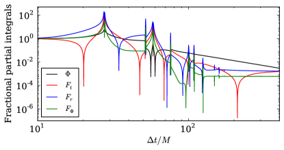
Figure 6: Fractional difference of the partial self-field and self-force components relative to the reference values in Haas and Poisson (2006) for a circular geodesic orbit at $r_{0}=6M$. See Fig.12 in Casals et al. (2013) for the corresponding plots of the actual partial self-field and self-force.

The RGF allows us distinguish which aspects of wave propagation in black hole spacetimes (caustic echoes or late-time backscattering) affect the self-field and self-force. Figure 6 shows the partial self-field and the self-force components for the circular geodesic orbit at $r_{0}=6M$ relative to the reference values $\Phi_{\rm reference}$ computed in Haas and Poisson (2006). The partial self-field is defined as the integral in Eq. (III.2) but with the lower limit of integration replaced by $-\Delta t$ as the independent variable in the figure. The fractional partial self-field is defined as

$$\bigg{|}1-\frac{\Phi_{\rm partial}(\Delta t)}{\Phi_{\rm reference}}\bigg{|}.$$ (39)

Similar definitions are taken for the fractional partial self-force components.

Most of the sharp features in Fig. 6 are caustic echoes intersecting the circular orbit. After $\sim 80M$ caustic echoes no longer appreciably affect the self-field while this occurs for the self-force components only after $\sim 150M$. This is roughly compatible with the structure of the RGF and its derivatives observed in the left column of Fig. 4. For this particular orbit we see from Fig. 4 that there are $8$ or $9$ caustic echoes within $\sim 150M$. The late-time tail from backscattering appears to have little influence, if any, on the radial and azimuthal self-force components as indicated by the plateaus after $\sim 150M$. However, the self-field and the time component of the self- force seem to depend more strongly on the late-time tail. In fact, the difference between the partial integral for $F_{t}$ and the reference value changes sign just after $200M$, as can be seen in Fig. 6 by the downward pointing spike. As a result, the partial $F_{t}$ value does not converge to its final value until late in the integration. The late-time tail itself has a strong influence on the self-field as the former changes the latter’s value by more than a factor of $30$ from $80M$ to $400M$. In addition, the self-field seems to have not yet converged after $400M$.

III.3 Geodesic eccentric orbits

Circular orbits are too special to be representative. For example, for circular orbits $\partial_{r}G_{\rm ret}(x,x^{\prime})=\partial_{r^{\prime}}G_{\rm ret}(x,x^{\prime})$ and one can avoid the careful treatment discussed in Sec. II.1.1 for computing the derivative of the Green function. To illustrate the flexibility of the RGF method, we now study a family of eccentric orbits, which are representative of generic orbits in Schwarzschild spacetime.

Bound geodesics of Schwarzschild spacetime are conveniently parametrized by their eccentricity, $e$, and semi-latus rectum, $p$. These can be defined in terms of the radial turning points of the orbit, the periastron ($r_{\rm min}$) and apastron ($r_{\rm max}$),

$$p=\frac{2r_{\rm min}r_{\rm max}}{M(r_{\rm min}+r_{\rm max})},\quad e=\frac{r_{\rm max}-r_{\rm min}}{r_{\rm max}+r_{\rm min}}.$$ (40)

The stable bound orbits are those for which $p\geq 6+2e$. The separatrix, defined by $p=6+2e$ separates the stable and unstable orbits and corresponds to the limiting case where the orbit comes in from apastron and spends an infinite amount of time whirling around periastron. In terms of this $p$–$e$ parametrization, the redshift factor for eccentric orbits is given by

$$z=\left(1-\frac{2M}{r}\right)\sqrt{\frac{p(p-3-e^{2})}{(p-2-2e)(p-2+2e)}}.$$ (41)

We focus on the portion of the $p$–$e$ parameter space corresponding to points along the separatrix. Fixing $p=6+2e$ and $r_{0}=6M$ we parametrize the orbits by their eccentricity $0\leq e\leq 1$ along with the choice of whether the radial motion is oriented inwards or outwards at $r_{0}=6M$. This family of geodesics are illustrated in Fig. 3.

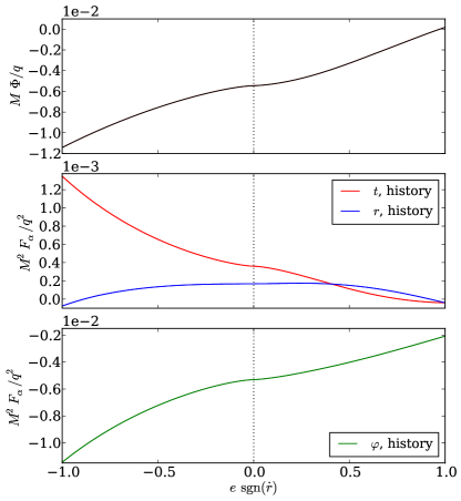
Figure 7: Regular part of the self-field and self-force on eccentric geodesic orbits along the separatrix $p=6+2e$ at the point when the orbital radius is $r_{0}=6M$. The orbits are parametrized by the eccentricity $e$ along with whether the motion is radially inward or outward, as measured by $\operatorname{sgn}\dot{r}$.

In Fig. 4 we plot the Green function (top, center) and its derivatives (bottom three, center) along the orbit for this family of geodesics. We find similar features to the accelerated circular orbits case, but the locations of the features are deformed as a result of the more complex orbital shape. This gives rise to qualitatively different results for the self-field and self-force, as illustrated in Fig. 7. In this case $\{\Phi,F_{t},F_{r},F_{\varphi}\}$ attain maximum and minimum values of approximately $\{0.0001839,0.001347,0.0001747,-0.002075\}\,q^{2}/M^{2}$ and $\{-0.01143,-0.00004040,-0.00007567,-0.01144\}\,q^{2}/M^{2}$, respectively, at eccentricities $e\operatorname{sgn}\dot{r}\approx\{1,-1,0.24,1\}$ and $e\operatorname{sgn}\dot{r}\approx\{-1,1,-1,-1\}$.

III.4 Radial infall

As a final example, we consider the unbound motion of a worldline falling radially inwards and compute the self-force at $r_{0}=6M$. Parametrizing the space of worldlines by the maximum radius $r_{\rm max}$ they attain, the position $r(t)$ at some time $\Delta t$ in the past is given by

$$\ddot{r}-\frac{2M}{r(r-2M)}\dot{r}^{2}+\frac{M(r-2M)^{2}}{r^{4}}\frac{r_{\rm max}}{(r_{\rm max}-2M)}=0,$$ (42)

where an overdot denotes differentiation with respect to Schwarzschild coordinate time. Once the motion reaches its maximum radius, $r_{\rm max}$, we hold its position fixed at $r=r_{\rm max}$ for the remainder of the time. This corresponds physically to a particle being held at rest at $r=r_{\max}$, then released and allowed to fall into the black hole.

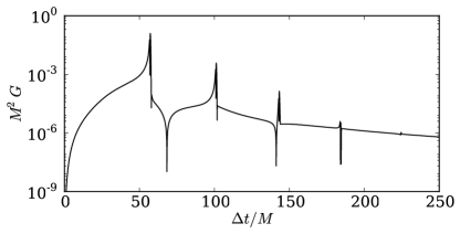
Figure 8: Green function along the worldline corresponding to a radial geodesic starting from rest at $r_{\rm max}=\infty$ and falling into $r_{0}=6M$. The two-fold singularity structure apparent in this case is in contrast to the standard four-fold structure which is typically seen for orbits in the Schwarzschild spacetime.

In Fig. 4 we plot the Green function along the worldline for this family of geodesics. One particularly interesting feature of this case is that the Green function no longer has the familiar four-fold structure of other orbits in Schwarzschild spacetime, but instead has a two-fold structure. This is due to the fact that, in this case, the singularities in the Green function always happen at caustics, where there is a $1$-parameter family of null geodesics crossing the worldline, rather than just a single null geodesic. This two-fold structure is clearly illustrated in Fig. 8, showing the case $r_{\rm max}=\infty$.

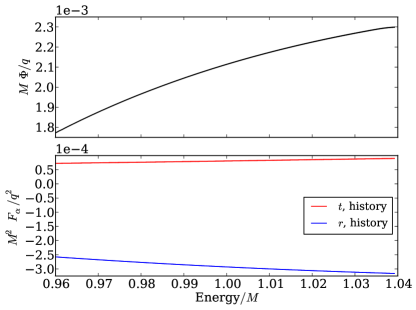
Figure 9: Regular part of the self-field and self-force on radial infall worldlines released from rest at different initial radii $r_{\rm max}$. The magnitude of the self-interaction increases as the energy of the motion is increased by increasing $r_{\rm max}$. The extrapolation to $r_{\rm max}=6M$ would correspond to the static case, where we would expect the self-interaction to be exactly $0$.

In Fig. 9 we plot the self-field and self-force as a function of the energy of the geodesic (which is directly related to $r_{\rm max}$). The symmetry of the problem demands $F_{\varphi}=0$ in all cases. Both the self-field and self-force are monotonic functions of the energy, with larger (in magnitude) values for more energetic worldlines. This behavior agrees with intuition; more energetic geodesics are moving faster and one could reasonably expect stronger self-interaction as a result.

IV Concluding remarks

We have presented a new method for numerically computing the self-force based on a global approximation of the RGF. The method takes advantage of the fact that the RGF is the fundamental solution to the wave equation in a curved background and can be used to build any inhomogeneous solution through a straightforward convolution integral with the source of interest. In this way, the quintessential features of wave propagation are disentangled from the arbitrary source.

Global numerical approximations for the RGF can be obtained in at least two ways: either by approximating the delta-distribution source by a Gaussian (as introduced in Zenginoglu and Galley (2012)) or using a Kirchhoff representation and approximating delta-distribution initial data by a Gaussian. In this paper we chose the latter and exploited the spherical symmetry of the Schwarzschild background to numerically solve the initial value problem as a system of uncoupled (1+1)-dimensional partial differential equations, one for each spherical-harmonic $\ell$ mode. The numerical solution was augmented with analytical approximations for the early-time Casals et al. (2009b) and late-time Casals and Ottewill (2012, 2014) behavior of the RGF.

IV.1 Advantages

The RGF approach introduced in this paper has several distinct advantages. First, the regular part of the self-field and the self-force are simply calculated by excluding the coincidence limit of the Green function when computing the worldline integrals in (5) and (6). This regularization procedure is valid for arbitrary worldlines, even accelerated ones. This feature should be compared to the regularization procedures used in the more established methods of mode-sum regularization and effective source. In both approaches the self-field and self-force are regularized using parameters in the former and an effective source in the latter. Both quantities must be derived and computed beforehand for the given worldline. In addition, calculating the effective source can involve a significant fraction of the numerical computing time.

Second, once the RGF has been computed for a given base point, we can compute the regular parts of the self-field and self-force for any worldline passing through that spacetime point, i.e. all geodesics as well as generic, accelerated worldlines. This remarkable feature is unique compared to mode-sum and effective source methods, which can only compute the self-force for one worldline at a time. In this aspect, our method is complementary to other methods. The worldline integration method gives the self-force for all worldlines but only at one base point, whereas mode-sum and effective-source methods compute the self-force at any point on a worldline but only for one worldline.

Third, our method admits geometrical interpretations and allows for quantitative comparisons between contributions from back-scattering and caustic echoes in determining the magnitude and sign of the self-field and self-force. Such a geometrical picture is lacking in other approaches to self-force computations. We anticipate this to carry through to gravitational self-force where one can make similar interpretations but only within the gauge choice made for the gravitational perturbations.

Fourth, our method allows for an offline/online decomposition of the problem. In the offline stage, we can devote as many computational resources as desired to produce a highly accurate numerical approximation of the RGF. The RGF can thus be computed accurately once and for all for a sufficient number of field and base points. With the global RGF available from the offline stage, the online stage involves only cheap convolution integrals to compute the self-field and the self-force on a given worldline. The offline/online decomposition is particularly advantageous when computing the RGF for a very narrow Gaussian where significant computational resources are necessary for computing the RGF but not for evaluating worldline integrals.

Fifth, and perhaps the most powerful advantage of our method, knowledge of the RGF and of the regular self-force equations in terms of the RGF allows for the computation of higher order self-force effects with little further work. For example, once the scalar RGF is known one can simply perform the worldline integrals in the formal second order self-force expressions Galley (2012a, b) to obtain the regular part of the second order self-force on an arbitrary worldline. In both mode-sum and effective source approaches the contributions at higher orders to the regularization parameters and effective source, respectively, need to be derived first, which is a nontrivial task, before nonlinear self-force computations can be performed.

IV.2 Challenges

We mention four main challenges for the future applications of the worldline integration method.

First, the computation of the RGF needs to be performed for each base point that a given worldline passes through. In practice, one would require only a sufficiently dense distribution of base points for which the symmetries of the background can be exploited. Nevertheless, the construction of such a distribution is computationally expensive and will require large memory storage. Depending on how similar the solutions are from one base point to another, it is likely that the full space of solutions (parameterized by the base point) admits a reduced representation that is spanned by a compact set of judiciously selected solutions. Such a representation can be found with the Reduced Basis Method Field et al. (2011). Further reduced-order modeling techniques can be implemented to effectively predict the RGF associated with an arbitrary base point using a surrogate model Field et al. (2013) in place of solving for the full wave equation separately for each base point. Surrogate models may provide a highly compressed and accurate representation of the full space of approximate Green functions, which are also inexpensive to evaluate. These methods offer a promising avenue for future work, to solve the otherwise prohibitive computational and memory storage requirements involved with approximating the RGF at many base points.

Second, obtaining increasingly accurate RGFs requires reducing the Gaussian width $\varepsilon$ and increasing the number of $\ell$ modes, which may become prohibitively expensive both in computing time and memory storage. In Sec. II.1.3 we showed that decreasing $\varepsilon$ improves the self-field and self-force as $\varepsilon^{2}$. Likewise, an increase in the number of $\ell$ modes yields an improvement that scales as $1/\ell^{2}$. This improvement stems primarily from the fact that at early times (within the normal neighborhood) the direct $U(x,x^{\prime})\delta(\sigma)$ part of the Hadamard form Green function, Eq. (7), is smeared out over the entire normal neighborhood by the finite sum over $\ell$ and contaminates the Green function in that region. A significant gain is therefore possible without decreasing $\varepsilon$ or increasing $\ell$, but by subtracting the $\ell$-decomposition of this direct part Nolan (2013); Casals and Nolan (2012) before summing over $\ell$. Another approach is to adapt numerical methods for high-frequency wave propagation such as the “frozen Gaussian approximation” Lu and Yang (2011) based on a paraxial approximation of the wave equation. Yet another is to supplement the numerical approximation of the RGF with (semi-)analytical high-frequency/large-$\ell$ methods such as the geometrical optics approximation discussed in Zenginoglu and Galley (2012), which was shown to capture the high-frequency behavior of the caustic echoes very accurately, and the large-$\ell$ asymptotics for the Green function multipolar modes, which accurately capture the global four-fold singularity structure Nolan (2013); Casals and Nolan (2012). These methods may provide a practical alternative to the brute force approach of reducing the Gaussian width.

Third, our method may not seem natural for computing self-consistent orbits as compared to, for example, the effective source method. The main challenge comes, again, from requiring the RGF at multiple base points. It should be possible to approximate the RGF at multiple base points for a self-consistent evolution by either using a sufficiently dense distribution of base points along with interpolation, or using the reduced order modeling techniques Field et al. (2011, 2013) discussed above.

Fourth, extending the method to compute gravitational self-force via the MiSaTaQuWa equation poses some technical challenges. The MiSaTaQuWa equation is formulated in terms of the derivatives of the Green function for a metric perturbation in Lorenz gauge. In Lorenz gauge, the metric perturbation on Schwarzschild spacetime may be decomposed in tensor spherical harmonics, leading to ten coupled 1+1D equations (or more precisely two sets, of 7 even and 3 odd-parity equations) Barack and Lousto (2005), which may be solved numerically with the methods described here. In principle, by starting with initial data in each component in turn, one may compute (an approximation to) the RGF and its derivatives. A naive method would require ten separate runs to compute the 100 components of the RGF, and computing derivatives of the RGF would require further runs with different initial data, as described in Sec. II.1.1. An additional challenge is posed by the low multipoles $\ell\leq 1$. These modes contain non-radiative physical content, related to the changes in mass and angular momentum of the system. In Lorenz gauge, initial-value formulations are also affected by linear-in-$t$ gauge mode instabilities in these modes, described in Sec. V of Ref. Dolan et al. (2013). A possible solution proposed there is to employ a generalized version of Lorenz gauge.

Unfortunately, in Lorenz gauge on Kerr spacetime the field equations cannot be separated into 1+1D form, and here we face a choice. Either we compute the RGF in Lorenz gauge by evolving multi-dimensional equations in the time domain (for example, the 2+1D approach of Ref. Dolan et al. (2013)), or we pursue a calculation in the radiation gauge Shah et al. (2011); Keidl et al. (2010); Shah et al. (2012). A key advantage of the latter approach is that the system is governed by ordinary differential equations. On the other hand, the radiation gauge calculation is highly technical (relying on Hertz potentials and metric reconstruction through application of linear differential operators) and is formulated entirely within the frequency domain, which would seem to negate the advantages of the time-domain approach developed here. Reformulating the MiSaTaQuWa equation to make use of radiation-gauge Green functions would present an additional challenge.

The resolution of these challenges should be the focus of future work to establish the worldline integration method as a practical and accurate approach to the self-force problem.