Testing the Perey Effect

Abstract

Background: The effects of non-local potentials have historically been approximately included by applying a correction factor to the solution of the corresponding equation for the local equivalent interaction. This is usually referred to as the Perey correction factor. Purpose: In this work we investigate the validity of the Perey correction factor for single-channel bound and scattering states, as well as in transfer $(p,d)$ cross sections. Method: We solve the scattering and bound state equations for non-local interactions of the Perey-Buck type, through an iterative method. Using the distorted wave Born approximation, we construct the T-matrix for $(p,d)$ on ¹⁷O, ⁴¹Ca, ⁴⁹Ca, ¹²⁷Sn, ¹³³Sn, and ²⁰⁹Pb at $20$ and $50$ MeV. Results: We found that for bound states, the Perey corrected wave function resulting from the local equation agreed well with that from the non-local equation in the interior region, but discrepancies were found in the surface and peripheral regions. Overall, the Perey correction factor was adequate for scattering states, with the exception of a few partial waves corresponding to the grazing impact parameters. These differences proved to be important for transfer reactions. Conclusions: The Perey correction factor does offer an improvement over taking a direct local equivalent solution. However, if the desired accuracy is to be better than 10%, the exact solution of the non-local equation should be pursued.

I Introduction

Optical potentials are a common ingredient in reaction studies. The optical model potential for nucleon-nucleus scattering has long been established as non-local Bell1959_PRL . While the vast majority of optical potentials found in the literature are assumed to be local and strongly energy dependent (i.e. Koning2003_NPA ; Varner1991_PR ), attempts have been made to determine non-local optical potentials Perey1962_NP ; Giannini1976_AP . Most often, optical potentials are phenomenologically based, fitted to elastic scattering. However, elastic scattering is predominantly an asymptotic process, so the short range details of the interaction cannot be uniquely constrained, particularly short-ranged non-local properties.

The predominant sources of non-locality in the effective nucleon-nucleus interaction arise from anti-symmetrization Canton2005_PRL ; Fraser2008_EPJ ; Rawitscher1994_PRC , multiple scattering Kerman1959_AP ; Crespo1996_PRC , and channel couplings Feshbach1958_AP ; Feshbach1962_AP . Jeukenne et al. developed a semi-microscopic formulation for the nucleon-nucleus optical potential based on the self-energy Jeukenne1974_PRC ; Jeukenne1977_PRC . This approach can provide good fits to elastic scattering data Bauge1998_PRC ; Bauge2001_PRC . Another approach consists on defining an optical potential based on the coupling of all inelastic channels to the elastic channel (the Feshbach channel coupling approach). These non-localities have been studied by Rawitscher Rawitscher1987_NPA . In either approaches, the resulting optical potential should be non-local, as well as energy dependent.

The precise form of the non-local potential is currently not known, and a number of forms have been considered (e.g. the parity-dependent potential of Cooper et al. Cooper1996_PRC and the velocity dependent potential Kisslinger1955_PR ; Zureikat2013_NPA ). In this work we consider the Perey-Buck form for the non-local potential Perey1962_NP ; Frahn1957_NC , which has energy and mass-independent potential parameters, and consists of a Woods-Saxon multiplied by a Gaussian which introduces the range of the non-locality. In Deltuva2009_PRC , the effect of non-locality of the Perey-Buck form is considered in deuteron induced reactions. Cross sections for various channels obtained when the nucleon-nucleus optical potentials are local CH89 Varner1991_PR differ considerably from those obtained using the non-local GR76 Giannini1976_AP . Since both CH89 and GR76 are global potentials with different fitting protocols, it is unclear whether the differences seen in Deltuva2009_PRC arise from the fact that these potentials are not phase equivalent, or genuinely from non-local effects. This deserves closer inspection.

Accounting for the non-locality through the energy dependence, as done for the local potentials, is known to be insufficient. One key feature of a non-local potential is that it reduces the amplitude of the wave function in the nuclear interior compared to the wave function from an equivalent local potential Austern1965_PR ; Fiedeldey1966_NP , the so-called Perey effect. Shortly after the introduction of the Perey-Buck potential, Austern studied the wave functions of non-local potentials and demonstrated the Perey effect in one-dimension Austern1965_PR . Subsequently, Fiedeldey did a similar study but in the three-dimensional case Fiedeldey1966_NP . Using a different method, Austern presented a way to relate wave functions obtained from non-local and local potentials in the three-dimensional case Austern1970_Book . Since then, non-local calculations have been avoided by using this Perey Correction Factor (PCF).

Recently, Timofeyuk and Johnson Timofeyuk2013_PRL ; Timofeyuk2013_PRC studied the effects of including an energy-independent non-local potential in $(d,p)$ reactions within the Adiabatic Distorted Wave Approximation (ADWA) Johnson1974_NPA . Non-locality was included approximately through expansions to construct a local equivalent potential and solving the corresponding local Schrödinger’s equation. They found that a Perey-Buck type non-locality can be effectively included in $(d,p)$ through a very significant energy shift in the evaluation of the local optical potentials to be used in constructing the deuteron distorted waves. This can impact cross sections dramatically, and calls for further investigations.

In this work, we determine the importance of non-local effects in the various components of a nuclear reaction process, and assess the validity of the PCF by studying a wide range of reactions, including neutron states bound to ¹⁶O, ⁴⁰Ca, ⁴⁸Ca, ¹²⁶Sn, ¹³²Sn, and ²⁰⁸Pb, and $(p,p)$ and $(p,d)$ on ¹⁷O, ⁴¹Ca, ⁴⁹Ca, ¹²⁷Sn, ¹³³Sn, and ²⁰⁹Pb at $20$ and $50$ MeV.

The paper is organized in the following way. In Sec. II we briefly describe the necessary theory. Numerical details can be found in Sec. III. The results are presented in Sec. IV, starting with a discussion of local equivalent potentials in Sec. IV.1 and of approximate local equivalent potentials in Sec. IV.2. We consider the effects of non-localities on scattering wave functions and ways to correct for non-localities in Sec. IV.3. The effects of non-localities on bound state wave functions are presented in Sec. IV.4. We then explore the effects of non-localities on transfer cross sections in Sec. IV.5. We discuss the connection of this work with other relevant studies in Sec. V. Finally, in Sec. VI, conclusions are drawn.

II Theoretical considerations

Let us consider a nucleon scattering off a composite nucleus. The effective interaction between the nucleon and the nucleus is a non-local optical potential. In this case, the two-body Schrödinger equation takes the form

$$\frac{\hbar^{2}}{2\mu}\nabla^{2}\Psi(\textbf{r})+E\Psi(\textbf{r})=U_{o}(\textbf{r})\Psi(\textbf{r})+\int U^{NL}(\textbf{r},\textbf{r}^{\prime})\Psi(\textbf{r}^{\prime})d\textbf{r}^{\prime}$$ (1)

where $\mu$ is the reduced mass of the nucleon-nucleus system, $E$ is the energy in the center of mass, $U_{o}(\textbf{r})$ is the local part of the potential, and $\Psi({\bf r})$ is the scattering wave function. A particular form of the non-local potential introduced by Frahn and Lemmer Frahn1957_NC is

$$U^{NL}(\textbf{r},\textbf{r}^{\prime})=U^{NL}_{WS}\left(\left|\frac{\textbf{r}+\textbf{r}^{\prime}}{2}\right|\right)\frac{\exp\left(-\left|\frac{\textbf{r}-\textbf{r}^{\prime}}{\beta}\right|^{2}\right)}{\pi^{3/2}\beta^{3}},$$ (2)

where, $\beta$ is the range of the non-locality, and typically takes on a value of $\approx 0.85$ fm. In this work, $U^{NL}_{WS}$ is of a Woods-Saxon form of the variable $\tfrac{1}{2}|\textbf{r}+\textbf{r}^{\prime}|$.

This type of potential was further investigated by Perey and Buck Perey1962_NP . Making the approximation $|\textbf{r}+\textbf{r}^{\prime}|\approx(r+r^{\prime})$ in $U^{NL}_{WS}$ allows for an analytic partial wave decomposition resulting in the partial wave equation

$$\frac{\hbar^{2}}{2\mu}\left[\frac{d^{2}}{dr^{2}}\right. - \left.\frac{\ell(\ell+1)}{r^{2}}\right]\psi^{NL}_{\ell}(r)+E\psi^{NL}_{\ell}(r)$$ (3)

$$= U_{o}(r)\psi^{NL}_{\ell}(r)+\int g_{\ell}(r,r^{\prime})\psi^{NL}_{\ell}(r^{\prime})dr^{\prime}.$$

Here, the kernel is explicitly given by:

$$g_{\ell}(r,r^{\prime})=\frac{2i^{\ell}z}{\pi^{\frac{1}{2}}\beta}j_{\ell}(-iz)\exp\left(-\frac{r^{2}+r^{\prime 2}}{\beta^{2}}\right)U^{NL}_{WS}\left(\frac{1}{2}(r+r^{\prime})\right),$$ (4)

where $j_{\ell}$ are spherical Bessel functions, and $z=2rr^{\prime}/\beta^{2}$. In our study, we assume the spin-orbit and Coulomb potentials are local, and therefore, $U_{o}(r)=V_{so}(r)+V_{\textrm{coul}}(r)$.

For a non-local potential of the Perey-Buck type, the depths of an approximate local equivalent potential can be found from the relations Perey1962_NP

$$V^{NL}_{v} = V^{Loc}_{v}\exp\left[\frac{\mu\beta^{2}}{2\hbar^{2}}\left(E-V_{c}+V^{Loc}_{v}\right)\right]$$

$$W^{NL}_{d} = W^{Loc}_{d}\exp\left[\frac{\mu\beta^{2}}{2\hbar^{2}}\left(E-V_{c}+V^{Loc}_{v}\right)\right].$$ (5)

Here, $V_{v}$ and $W_{d}$ are the depths of the real volume and imaginary surface terms in the Woods-Saxon potential, respectively, and are positive constants. $E$ is the center of mass energy, and $V_{c}$ is the Coulomb potential at the origin for a solid uniformly charged sphere with radius $R_{c}=r_{c}A^{1/3}$. Notice that even though the non-local potential is energy-independent, the transformed local depths are energy-dependent, which is a common feature of local global optical potentials.

Through use of Eq.(II) and fits to neutron elastic scattering data on ²⁰⁸Pb at low energies, the Perey-Buck non-local potential was determined: the corresponding parameters are given in the first column of Table 1. The parameters in the Perey-Buck potential are both energy and mass-independent.

For a given non-local potential, a local equivalent potential can often be found. However, in the nuclear interior, the wave function resulting from using a non-local potential is reduced compared to the wave function resulting from using a local equivalent potential. This phenomenon is known as the Perey effect Austern1965_PR . Correcting for the reduced amplitude is done via the PCF:

$$F(r)=\left[1-\frac{\mu\beta^{2}}{2\hbar^{2}}\left(U^{LE}(r)-U_{o}(r)\right)\right]^{-1/2}.$$ (6)

Note that here, $U^{LE}(r)$ is the local equivalent potential. As we required the spin-orbit and Coulomb terms to be identical in the local and non-local potentials, these terms in $U^{LE}$ exactly cancel $U_{o}$. Since $F(r)\rightarrow 1$ as $r\rightarrow\infty$, the correction factor Eq.(6) only affects the magnitude of the wave function within the range of the nuclear interaction. A derivation of Eq.(II) and Eq.(6) is given in Appendix A.

In the asymptotic limit, the wave function takes the form

$$\psi^{\textrm{asym}}_{\ell}(r)=\frac{i}{2}\left[H^{-}_{\ell}(\eta,kr)-\textbf{S}_{\ell j}H^{+}(\eta,kr)\right],$$ (7)

where $\eta=Z_{1}Z_{2}e^{2}\mu/\hbar^{2}k$ is the Sommerfeld parameter, $k$ is the wave number, $\textbf{S}_{\ell j}$ is the scattering matrix element, and $H^{-}$ and $H^{+}$ are incoming and outgoing spherical Hankel functions, respectively. For neutrons, $\eta=0$.

In Sec. IV.5, we use the Distorted Wave Born Approximation (DWBA) to calculate the T-matrix for the B$(p,d)$A reaction, which, neglecting the remnant term, is written as

$$T_{p,d}=\langle\psi_{dA}^{(-)}\phi_{d}|V_{np}|\psi_{pB}\phi_{nA}\rangle\;,$$ (8)

where $\psi_{dA}^{(-)}$ is the deuteron scattering wave function, $\phi_{d}$ is the deuteron bound state, $V_{np}$ is the Reid soft core $np$ interaction Reid1968_AP , $\psi_{pB}$ is the proton distorted wave, and $\phi_{nA}$ is the neutron bound state wave function. (for details on the formalism, please check Thompson2009_Book ).

Due to its simplicity, a common technique is to do a calculation with a suitable local equivalent potential, then introduce the non-locality by modifying the wave function with the PCF

$$\psi^{PCF}_{\ell}(r)=F(r)\psi^{Loc}_{\ell}.$$ (9)

This is precisely the approach we want to test in this study.

III Numerical details

In this systematic study, we consider elastic scattering $(p,p)$ on ¹⁷O, ⁴¹Ca, ⁴⁹Ca, ¹²⁷Sn, ¹³³Sn, and ²⁰⁹Pb at $20$ and $50$ MeV and the wave functions for a neutron bound to ¹⁶O, ⁴⁰Ca, ⁴⁸Ca, ¹²⁶Sn, ¹³²Sn, and ²⁰⁸Pb. In both cases, the full non-local equation is solved using the Perey-Buck potential, with the method described in Appendix B.

For the scattering process, a local equivalent potential is determined by fitting the elastic scattering generated from the non-local equation. This was done using the code sfresco fresco . Using the local equivalent potential, the local scattering equation is solved to obtain $\psi^{Loc}$ and, finally, the PCF is applied to the wave function Eq.(9). The corrected wave function, $\psi^{PCF}$, is then compared to the solution of the full non-local equation, $\psi^{NL}$.

A similar procedure is followed for the bound states. The full non-local equation is solved using a real Woods-Saxon form with radius $r=1.25$ fm, diffuseness $a=0.65$ fm, and a non-locality parameter $\beta=0.85$ fm. The depth is then adjusted to reproduce the physical binding energy of the system. The local equation is solved with the local depth $V_{ws}^{Loc}$ necessary to reproduce the binding energy. We then apply the PCF to the resulting wave function, and renormalize to unity, to obtained the corrected bound state. The corrected wave function, $\phi^{PCF}$, is then compared to the solution of the full non-local equation, $\phi^{NL}$.

The bound and scattering states resulting from either non-local or local potentials are then introduced into the DWBA T-matrix for $(p,d)$, Eq.(8), for describing the process at $20$ and $50$ MeV. Angular distributions are calculated using the code fresco fresco . Non-locality was only added in the entrance channel, namely through the proton distorted wave and the neutron bound state. The local global parameterization of Daehnick et al. was used to obtain $\psi_{dA}$ in the exit channel. The scattering wave functions were solved by using a $0.05$ fm radial step size with a matching radius of $40$ fm. For the bound state solutions, we used a radial step size of $0.02$ fm. The matching radius was half the radius of the nucleus under consideration, and the maximum radius was $30$ fm, except for a very low binding energy study, when a larger value was necessary. The cross sections contain contributions of partial waves up to $J=30$.

In the following subsection, we present the results and analyze the effect of non-locality and the approximate correction factor in detail.

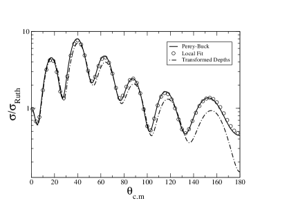
Figure 1: ⁴⁹Ca$(p,p)^{49}$Ca at $50.0$ MeV: the solid line is obtained from solving Eq.(3), the open circles are a fit to the non-local solution, and the dot-dash line is obtained by transforming the depths of the volume and surface potentials according to Eq.(II).

IV Results

IV.1 Local Equivalent Potentials

As described before, in order to study the correction factor, a local equivalent potential (LEP) needs to be found. A local potential is equivalent to a given non-local potential if it produces the same S-matrix elements, thus, producing the same elastic scattering angular distribution. A LEP is found by $\chi^{2}$ minimization starting from the transformed local potential obtained by using Eq.(II). We required that the spin-orbit and Coulomb terms of the Perey-Buck non-local potential and the LEP be exactly the same, thus only the real volume and imaginary surface terms were allowed to vary in the fit to find the LEP (a total of 6 parameters). For most cases we were able to obtain a near perfect fit. We demonstrate the procedure with the elastic scattering of protons on ⁴⁹Ca at 50 MeV. The ratio to Rutherford angular distributions are shown in Fig.1 for the case of the Perey-Buck non-local potential (solid line) and the LEP (circles). The angular distribution for the LEP sits on top of the one obtained from Perey-Buck, as it should.

IV.2 Transformed Local Equivalents

In order to obtain the LEP, we first had to solve the non-local equation, which in the past was too demanding computationally. Instead, the transformations shown in Eq.(II) were sometimes used. We consider again the case of ⁴⁹Ca$(p,p)^{49}$Ca at $50$ MeV. Table 1 contains the original Perey-Buck potentials, the transformed potentials and the LEP. The subscripts $v$, $d$, $so$, and $c$ denote the real volume, imaginary surface, spin-orbit, and Coulomb terms of the potential, respectively. $V_{v}$, $W_{v}$ and $V_{so}$ are the depths of the potentials in MeV. The radius parameter, $r$, is used to find the radius of the nucleus under consideration through the formula $R=rA^{1/3}$, and $a$ is the diffuseness of the Woods-Saxon potential.

	Perey-Buck	Transformed	Local Fit
$V_{v}$ (MeV)	71.000	37.151	37.842
$r_{v}$ (fm)	1.220	1.220	1.251
$a_{v}$ (fm)	0.650	0.650	0.629
$W_{d}$ (MeV)	15.000	7.849	8.697
$r_{d}$ (fm)	1.220	1.220	1.236
$a_{d}$ (fm)	0.470	0.470	0.440
$V_{so}$ (MeV)	7.180	7.180	7.180
$r_{so}$ (fm)	1.220	1.220	1.220
$a_{so}$ (fm)	0.650	0.650	0.650
$r_{c}$ (fm)	1.220	1.220	1.220

Table 1: Potential parameters for the reaction ⁴⁹Ca$(p,p)^{49}$Ca at $50.0$ MeV: the first column are the parameters for the Perey-Buck non-local potential (the range of the non-locality in the Perey-Buck potentials is fixed $\beta=0.85$ fm), the second column corresponds to the local potential where the depths of the real volume and imaginary surface terms were transformed according to Eq.(II), and the third column are the parameters for the local fit to the elastic distribution generated with the Perey-Buck potential.

Table 1 shows that the depths of the transformed local potential and the local fit are in fair agreement. In the local fit, the depth, radius, and diffuseness are adjusted for a better fit, while for the transformed local potential, the radius and diffuseness are the same as in the Perey-Buck potential. The dot-dashed line in Fig. 1 depicts the elastic scattering obtained from the transformed potential. Aside from significant discrepancies at large angles, the transformed local potential does a fair job in reproducing the non-local elastic cross section. However, using this transformation formula to construct a potential should be treated with caution, since the fact that the radius and diffuseness are unchanged does not allow for a correct description of the diffraction pattern.

IV.3 Corrections to Scattering Wave Functions

Once the LEP solution $\psi^{Loc}(r)$ is found, the PCF can be tested by comparing it to the solution to the full non-local equation, $\psi^{NL}(r)$, and the corrected wave function, $\psi^{PCF}(r)$.

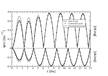
Figure 2: The real and imaginary parts of the $J^{\pi}=0.5^{-}$ partial wave of the scattering wave function for the reaction ⁴⁹Ca$(p,p)^{49}$Ca at $50.0$ MeV: $\psi^{NL}$ (solid line), $\psi^{PCF}$ (crosses) and $\psi^{Loc}$ (dashed line). Top (bottom) panel: absolute value of the real (imaginary) part of the scattering wave function.

For all cases investigated, the non-local wave function and the PCF corrected local wave function agree well for most partial waves. An example is provided in Fig.2. $\psi^{NL}$ (solid line) is reduced in the interior compared to $\psi^{Loc}$ (dashed line) but PCF accounts well for this reduction as shown by $\psi^{PCF}$ (crosses). However, in all cases, problems arose for partial waves corresponding to impact parameters around the surface region, as illustrated in Fig.3. The differences for these angular momenta are particularly relevant for transfer cross sections, which tend to be most sensitive to the surface region. The weaker performance of the PCF for partial waves corresponding to the surface is partly due to neglecting the $\nabla^{2}F$ term in the derivation of Eq.(6), which only contributes in the surface region (See Appendix A).

Occasionally we found slight differences in the asymptotic region due to small differences in the S-Matrix elements for a particular partial wave. Since the wave functions are normalized according to Eq.(7), small changes in the S-Matrix will result in different amplitudes for the real and imaginary parts of the scattering wave function in the asymptotic region.

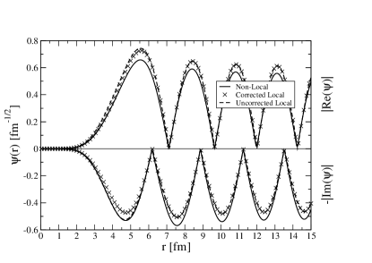
Figure 3: The real and imaginary parts of the $J^{\pi}=5.5^{+}$ partial wave of the scattering wave function for the reaction ⁴⁹Ca$(p,p)^{49}$Ca at $50.0$ MeV (see caption of Fig.2).

IV.4 Bound State Wave Functions

For the bound state case, the non-local and local equivalent potentials were chosen so that the correct binding energy was reproduced. Non-local volume and local spin-orbit terms were included. Only the depth of the central volume potential was varied to reproduce the binding energy. Since neutron bound states are of interest in $(d,p)$ and $(p,d)$ reactions, only these were considered. Like in the scattering case, Eq.(6) was used to correct the local wave function for non-locality. After the local wave function was corrected, the resulting wave function was renormalized. It is very important to renormalize the corrected wave function after applying Eq.(6). If the bound wave function is not normalized after applying the PCF, the resulting corrected wave function is worse than the uncorrected wave function.

The $2p_{3/2}$ ground state wave function for $n+^{48}$Ca is shown in Fig.4. Visually, the correction factor does an adequate job correcting for non-locality in the bound state. However, in the region between the two peaks of the wave function ($2-5$ fm), the PCF does very little to bring the local wave function into agreement with the non-local wave function. The inset in Fig.4 shows the difference between $\phi^{NL}$ and $\phi^{PCF}$ as a function of r. The bound wave function has a large slope in this region, so the percent difference between the non-local and corrected local wave functions can be large. Also, the amplitude in the asymptotic region of the local wave functions are smaller than the amplitude of $\phi^{NL}$. As we shall discuss next, in Section IV.5, these features influence the $(p,d)$ transfer cross section in different ways.

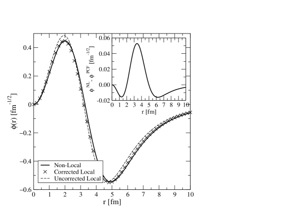
Figure 4: The ground state, $2p_{3/2}$, bound wave function for $n+^{48}$Ca (see caption of Fig.2). The inset shows the difference $\phi^{NL}-\phi^{PCF}$.

IV.5 Transfer Cross Sections

We now turn our attention to the transfer $(p,d)$ cross sections. In Fig.5 the $(p,d)$ transfer cross section for ⁴⁹Ca$(p,d)^{48}$Ca at 50.0 MeV in the proton laboratory frame is shown. The solid line corresponds to including non-locality in both the proton distorted wave and the neutron bound state, the dashed line corresponds to the distribution obtained when only local equivalent interactions are used, and the crosses correspond to the cross sections obtained when the proton scattering state and the neutron bound state are both corrected by the PCF. While the Perey correction improves upon the distribution involving local interactions only, it is still unable to fully capture the complex effect of non-locality. The prominent changes at zero degrees was unique to this case, but the very significant changes around the main peak was seen for most distributions studied.

We also show the separate effect of including only non-locality in the proton scattering state (dotted) and the neutron bound state (dot-dashed). For this case, the non-locality in the proton distorted wave acts in a similar way to the non-locality in the bound state, namely it increases the cross section at zero degrees and reduces the cross section around $15^{\circ}$.

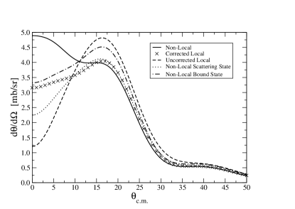
Figure 5: Angular distributions for ⁴⁹Ca$(p,d)^{48}$Ca at $50.0$ MeV: inclusion of non-locality in both the proton distorted wave and the neutron bound state (solid line), using LEP, then applying the correction factor to both the scattering and bound states (crosses), using the LEP without applying any corrections (dashed line); including non-locality only to the proton distorted wave (dotted line), and including non-locality in the neutron bound state only (dot-dashed line).

The reason for the large changes at small angles can be seen from an analysis of the scattering and bound wave functions of Figs. 2, 3, and 4. The existence of a node in the bound state wave function influences the cross section in a complex manner. The radius that corresponds to the surface for ⁴⁹Ca occurs at a radius slightly larger than that where the bound state wave function is zero. The bound wave function has a large slope in this region, so the percent difference between the non-local and local wave functions can be quite large in this region. For this case, the non-local bound wave function is smaller than the local wave functions in this region, reducing the cross section at the peak. On the other hand, the magnitude of the bound wave function is larger for the non-local case in the tail region, which enhances the cross section at forward angles.

For the scattering wave functions, the largest differences were for partial waves that corresponded to the surface. Also, the asymptotics of scattering partial waves were different due to small differences in the S-Matrix, mostly for surface partial waves. The larger the amplitude in the asymptotic region, the larger the cross section at forward angles. There is an interplay between the real and imaginary parts of the scattering wave function which influences the cross section at forward angles. In a very complex manner, the combination of all these effects produces the interesting behavior of the transfer cross section at forward angles, and the changes in the magnitude of the cross section at the peak for this particular reaction.

In order to better understand this case, we artificially modified the bound wave function. By changing the binding energy we altered the Q-value of the reaction. Different Q-values produced very different types of distributions, both in shape and in magnitude. Nevertheless, similar dramatic changes in the cross section due to non-locality were found. For very low binding energy, the normalization of the bound wave function was dominated by the asymptotics, so the PCF did very little. The node in the wave function altered the cross section in a very complex way. The PCF was not able to correct the bound wave function in the region around the node since the wave function and the PCF have a very large slope in this region, so inadequacies of the PCF were amplified.

Consider now the same target but lower energy. In Fig.6 we present the transfer angular distribution for ⁴⁹Ca$(p,d)^{48}$Ca at $20.0$ MeV. Non-locality is seen to have a large effect at small angles. Including non-locality in only the bound state increases the cross section at forward angles, which is to be expected from Fig.4, where it is seen that the magnitude of $\phi_{nA}^{NL}$ is larger than $\phi_{nA}^{PCF}$ and $\phi_{nA}^{Loc}$ in the asymptotic region. Non-locality in only the scattering state decreases the cross section, but only by a small amount. The net effect of non-locality is an overall increase in the cross section of $17.3\%$ relative to the cross section obtained with local interactions only. While the correction factor moves the transfer distribution in the right direction, it falls short by $5.2\%$.

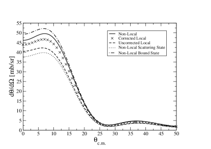
Figure 6: Angular distributions for ⁴⁹Ca$(p,d)^{48}$Ca at $20.0$ MeV (descriptions of each line is given in the caption of Fig.5).

Next we consider some heavier targets, ¹³³Sn and ²⁰⁹Pb, and study $(p,d)$ at $20$ MeV. In both cases, the inclusion of non-locality in the scattering state decreases the cross section by a small amount. This is due to the low energy of the proton, and the high charge of the target; the details of the scattering wave function within the nuclear interior are not significant for the transfer since these details are suppressed by the Coulomb barrier. Non-locality in the bound state is very significant, and increases the cross section by a large amount in both cases. In ¹³³Sn, the correction factor does a fair job taking non-locality into account, but there is still a noticeable discrepancy between the full non-local and corrected local results. In ²⁰⁹Pb, there are discrepancies at forward angles, but coincidentally the distributions resulting from the non-local potential and the local potential with the PCF agree quite well at the major peak of the distribution. This agreement is accidental and comes from the non-local effect in the bound state canceling that in the scattering state.

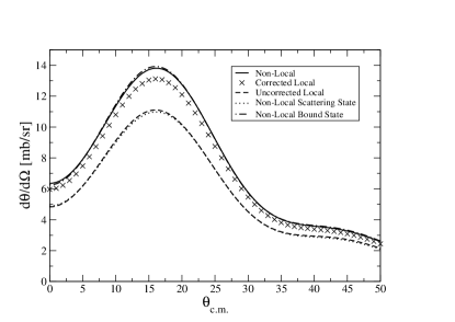
Figure 7: Angular distributions for ¹³³Sn$(p,d)^{132}$Sn at $20.0$ MeV (descriptions of each line is given in the caption of Fig.5).

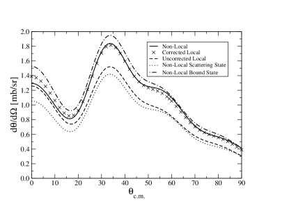
Figure 8: Angular distributions for ²⁰⁹Pb$(p,d)^{208}$Pb at $20.0$ MeV (descriptions of each line is given in the caption of Fig.5).

The percent differences at the first peak of the transfer distributions for all the cases that were studied are summarized in Table 2 and 3 for the $(p,d)$ reactions at $20$ and $50$ MeV.

	Corrected	Non-Local
$E_{lab}=20$ MeV	Relative to Local	Relative to Local
17O$(1d_{5/2})(p,d)$	$7.1\%$	$18.8\%$
17O$(2s_{1/2})(p,d)$	$20.1\%$	$26.5\%$
41Ca$(p,d)$	$11.4\%$	$21.9\%$
49Ca$(p,d)$	$10.4\%$	$17.3\%$
127Sn$(p,d)$	$17.5\%$	$17.3\%$
133Sn$(p,d)$	$18.2\%$	$24.4\%$
209Pb$(p,d)$	$19.4\%$	$20.8\%$

Table 2: Percent difference of the $(p,d)$ transfer cross sections at the first peak when using Eq.(6) (2nd column), or a non-local potential (3rd column), relative to the local calculation with the LEP, for a number of reactions occurring at $20$ MeV.

	Corrected	Non-Local
$E_{lab}=50$ MeV	Relative to Local	Relative to Local
17O$(1d_{5/2})(p,d)$	$17.0\%$	$35.4\%$
17O$(2s_{1/2})(p,d)$	$0.2\%$	$12.7\%$
41Ca$(p,d)$	$2.9\%$	$5.8\%$
49Ca$(p,d)$	$-16.0\%$	$-17.1\%$
127Sn$(p,d)$	$10.1\%$	$4.5\%$
133Sn$(p,d)$	$-6.7\%$	$-16.9\%$
209Pb$(p,d)$	$8.6\%$	$8.6\%$

Table 3: Percent difference of the $(p,d)$ transfer cross sections at the first peak when using Eq.(6) (2nd column), or a non-local potential (3rd column), relative to the local calculation with the LEP, for a number of reactions occurring at $50$ MeV.

It is seen that for both energies and for nearly all cases, the inclusion of non-locality in the entrance channel can have a very significant effect on the transfer cross section, often times introducing differences of $15-35\%$. Most of the time, adding non-locality increases the cross section at the first peak. In general, the correction factor moves the distribution obtained with local interactions in the direction of the distribution including the non-local interactions. In the case of ¹²⁷Sn$(p,d)$ at $50$ MeV, the correction factor overshoots at the first peak, but the overall shape of the corrected distribution is in better agreement with the exact result.

V Discussion

It should be noted that the PCF is only valid for non-local potentials of the Perey-Buck form. However, there is no reason to expect that the full non-locality in the optical potential will look anything like the Perey-Buck form. On physical grounds, the optical potential must be energy dependent due to non-localities arising from channel couplings. While the specific form chosen for the Perey-Buck potential is convenient for numerical calculations, a single Gaussian term mocking up all energy-independent non-local effects is likely to be an oversimplification.

In an earlier study, Rawitscher et al. Rawitscher1994_PRC calculated the exchange non-locality in $n-^{16}$O scattering and examined the PCF. The wave functions obtained from their microscopically derived exchange non-locality were reasonably corrected by the PCF. The exchange non-locality is based on anti-symmetrized wave functions, which will naturally reduce the amplitude of the wave function in the nuclear interior due to the Pauli exclusion principle, similarly to the PCF. Results in Rawitscher1994_PRC show that the PCF is able to approximately take into account the effects of including exchange. In another study by Rawitscher Rawitscher1987_NPA , the microscopic Feshbach optical potential from channel coupling is examined. The resulting potentials were strongly $\ell-$dependent, had emissive (positive imaginary) parts, and the non-local part did not resemble a Gaussian shape. The PCF obtained from the Wronskian was also strongly angular momentum dependent, and was found to be larger than unity in some cases. The channel coupling non-locality is therefore very different than the exchange non-locality, and one should not expect it to be corrected for in the same way. In those studies Rawitscher1994_PRC ; Rawitscher1987_NPA , the exchange and channel coupling non-localities were analyzed separately. To the authors knowledge, no study has examined the simultaneous inclusion of exchange and channel coupling non-localities.

Our results, together with Rawitscher1994_PRC ; Rawitscher1987_NPA , emphasize the need for non-locality to be treated explicitly, contrary to what has been preferred for more than 50 years. Since we have not yet found a good way to pin down non-locality phenomenologically, it would be extremely helpful to have microscopically derived optical potentials to guide further work. Microscopic $nA$ optical potentials based on the nucleon-nucleon interaction are particularly attractive because they immediately connect the intrinsic structure of the target to the reaction.

VI Conclusions

The long established Perey correction factor (PCF) was studied. To do so, the integro-differential equation containing the Perey-Buck non-local potential was solved numerically for single channel scattering and bound states. A local equivalent potential was obtained by fitting the elastic distribution generated by the Perey-Buck potential to a local potential. Both the local and non-local binding potentials reproduced the experimental binding energies. The scattering and bound state wave functions were used in a finite range DWBA calculation in order to calculate $(p,d)$ transfer cross sections. The PCF was applied to the wave functions generated with the local equivalent potentials.

For the $(p,d)$ transfer reactions, we found that the explicit inclusion of non-locality to the entrance channel increased the transfer distribution at the first peak by $15-35\%$. The transfer distribution from using a non-local potential increased relative to the distribution from the local potential in most cases. In all cases, the PCF moved the transfer distribution in the direction of the distribution which included non-locality explicitly. However, non-locality was never fully taken into account with the PCF.

ACKNOWLEDGEMENT

We are grateful to Jeff Tostevin for countless discussions and invaluable advice. We would also like to thank Nicolas Michel and Ron Johnson for many useful suggestions. This work was supported by the National Science Foundation under Grant No. PHY-0800026 and the Department of Energy under Contracts No. DE-FG52-08NA28552 and No. DE-SC0004087.

Appendix A Deriving the Perey correction factor

Here we provide details on the derivation of the PCF, Eq.(6). We also include the derivation of the transformation formulas Eq.(II), as well as the correct radial version of the transformation formulas which could be used to transform the non-local radius and diffuseness to their local counterpart.

We start from Eq.(1). Let us define a function $F(\textbf{r})$ that connects the local wave function $\Psi^{Loc}(\textbf{r})$, resulting from the potential $U^{LE}(\textbf{r})$, with the wave function resulting from a non-local potential, $\Psi^{NL}(\textbf{r})$

$${}\Psi^{NL}(\textbf{r})\equiv F(\textbf{r})\Psi^{Loc}(\textbf{r}).$$ (10)

Since the local and non-local equations describe the same elastic scattering, the wave functions should be identical outside the nuclear interior. Thus, $F(\textbf{r})\rightarrow 1$ as $r\rightarrow\infty$. By inserting Eq.(10) into the non-local equation Eq.(1) we can reduce the result to the following local equivalent equation

$$-\frac{\hbar^{2}}{2\mu}\nabla^{2}\Psi^{Loc}(\textbf{r})+U^{LE}(\textbf{r})\Psi^{Loc}(\textbf{r})=E\Psi^{Loc}(\textbf{r}),$$ (11)

where the local equivalent potential is given by:

$$U^{LE}(\textbf{r}) = \frac{-\frac{\hbar^{2}}{\mu}\nabla F(\textbf{r})\cdot\nabla\Psi^{Loc}(\textbf{r})-\frac{\hbar^{2}}{2\mu}(\nabla^{2}F(\textbf{r}))\Psi^{Loc}(\textbf{r})}{F(\textbf{r})\Psi^{Loc}(\textbf{r})}$$

$$+\frac{\int U^{NL}(\textbf{r},\textbf{r}^{\prime})F(\textbf{r}^{\prime})\Psi^{Loc}(\textbf{r}^{\prime})d\textbf{r}^{\prime}}{{F(\textbf{r})\Psi^{Loc}(\textbf{r})}}+U_{o}(\textbf{r}).$$

We next consider the second term of Eq.(A3) and introduce the explicit non-local potential form of Eq.(2). Using the definition $\textbf{s}=\textbf{r}-\textbf{r}^{\prime}$, expanding in powers of $s$ up to first order, the integral becomes

$$\int U^{NL}_{WS}\left(\left|\textbf{r}-\frac{1}{2}\textbf{s}\right|\right)H(s)F(\textbf{r}-\textbf{s})\Psi^{Loc}(\textbf{r}-\textbf{s})d\textbf{s}$$ (13)

$$\approx U_{WS}^{NL}(r)F(r)\int H(s)\Psi^{Loc}(\textbf{r}-\textbf{s})d\textbf{s}$$

$$-\frac{1}{2}F(r)\nabla U_{WS}^{NL}(\textbf{r})\cdot\int\textbf{s}H(s)\Psi^{Loc}(\textbf{r}-\textbf{s})d\textbf{s}$$

$$-\ U_{WS}^{NL}(r)\nabla F(\textbf{r})\int\textbf{s}H(s)\Psi^{Loc}(\textbf{r}-\textbf{s})d\textbf{s}$$

where

$$H(s)=\frac{\exp\left(-\frac{s^{2}}{\beta^{2}}\right)}{\pi^{3/2}\beta^{3}}.$$ (14)

Therefore, the local equivalent potential becomes:

$$U^{LE}(\textbf{r}) \approx \frac{1}{F(\textbf{r})\Psi^{Loc}(\textbf{r})}\left[-\frac{\hbar^{2}}{\mu}(\nabla F\cdot\nabla\Psi^{Loc})\right.$$ (15)

$$+\ \left.U^{NL}_{WS}(r)F(r)\int H(s)\Psi^{Loc}(\textbf{r}-\textbf{s})d\textbf{s}\right.$$

$$-\ \left.\frac{1}{2}F(r)\nabla U^{NL}_{WS}\cdot\int\textbf{s}H(s)\Psi^{Loc}(\textbf{r}-\textbf{s})d\textbf{s}\right.$$

$$-\ \left.U^{NL}_{WS}(r)\nabla F\cdot\int\textbf{s}H(s)\Psi^{Loc}(\textbf{r}-\textbf{s})d\textbf{s}\right]$$

$$-\ \frac{\hbar^{2}}{2\mu}\frac{\nabla^{2}F(\textbf{r})}{F(\textbf{r})}+U_{o}(\textbf{r}).$$

Consider the four terms in the brackets. All of these terms are divided by $\Psi^{Loc}$, which has nodes. The first, third, and fourth terms depend on dot products and gradients of $\Psi^{Loc}$. These terms are unlikely to individually equal zero when $\Psi^{Loc}$ in the denominator equals zero. Thus, we require that these terms sum to zero so that $U^{LE}(\textbf{r})$ remains finite. As pointed out in Austern1970_Book , this is not an approximation, but merely a condition for the method to work. Applying this condition gives us two equations:

$$U^{LE}(\textbf{r}) = U^{NL}_{WS}(r)\left[\frac{\int H(s)\Psi^{Loc}(\textbf{r}-\textbf{s})d\textbf{s}}{\Psi^{Loc}(\textbf{r})}\right]$$ (16)

$$+U_{o}({\bf r})-\frac{\hbar^{2}}{2\mu}\frac{\nabla^{2}F(\textbf{r})}{F(\textbf{r})}$$

$$0 = \frac{\hbar^{2}}{\mu}(\nabla F\cdot\nabla\Psi^{Loc})+\left[\frac{1}{2}F(r)\nabla U^{NL}_{WS}+U^{NL}_{WS}(r)\nabla F\right]$$ (17)

$$\cdot\int\textbf{s}H(s)\Psi^{Loc}(\textbf{r}-\textbf{s})d\textbf{s}.$$

Instead of using the local WKB approximations as in Austern Austern1970_Book , we use the operator form of the Taylor expansion to factorize the wave function:

$$\Psi^{Loc}(\textbf{r}-\textbf{s})=e^{-i\textbf{s}\cdot\textbf{k}}\Psi^{Loc}(\textbf{r}),$$ (18)

with $\textbf{k}=-i\nabla$. This simplifies the integrals in Eq.(16) and Eq.(17). Consider first the integral in Eq.(16)

$$\int H(s)\Psi^{Loc}(\textbf{r} - \textbf{s})d\textbf{s}=\left[\int e^{-i\textbf{s}\cdot\textbf{k}}H(s)d\textbf{s}\right]\Psi^{Loc}(\textbf{r})$$ (19)

$$= \exp\left[\frac{-k^{2}\beta^{2}}{4}\right]\Psi^{Loc}(\textbf{r}).$$

Therefore, assuming the potentials are scalar functions of $r$, and replacing Eq.(19) into Eq.(16) we obtain;

$$U^{LE}(r) = U^{NL}_{WS}(r)\exp\left[{-\frac{\mu\beta^{2}}{2\hbar^{2}}\left(E-U^{LE}(r)\right)}\right]$$ (20)

$$+U_{o}(r)-\frac{\hbar^{2}}{2\mu}\frac{\nabla^{2}F(r)}{F(r)},$$

where we used $k^{2}=-\nabla^{2}$ in the exponent to first order, and the Schrödinger’s equation. Making the replacement $U^{LE}(r)=U^{Loc}_{WS}(r)+U_{o}(r)$, gives us the radial transformation formula

$$U_{WS}^{NL}(r) = \left(U_{WS}^{Loc}(r)+\frac{\hbar^{2}}{2\mu}\frac{\nabla^{2}F(r)}{F(r)}\right)$$

$$\times\exp\left[\frac{\mu\beta^{2}}{2\hbar^{2}}\left(E-U_{WS}^{Loc}(r)-U_{o}(r)\right)\right].$$

The $\nabla^{2}F$ term is significant around the surface, but near the origin this term is negligible. Therefore, if we neglect this term, then we must remove the radial arguments, and consider this formula only near the origin. Therefore, for $r\approx 0$

$$U_{WS}^{NL}(0)\approx U_{WS}^{Loc}(0)\exp\left[\frac{\mu\beta^{2}}{2\hbar^{2}}\left(E-U_{WS}^{Loc}(0)-U_{o}(0)\right)\right].$$ (22)

The $U_{WS}(r)$ functions are of a Woods-Saxon form, and have real and imaginary parts

$$U_{WS}(r) = U_{R}(r)+iU_{I}(r)$$

$$= \frac{-V_{v}}{1+\exp\left(\frac{r-R}{a}\right)}+4i\frac{-W_{d}\exp\left(\frac{r-R}{a}\right)}{\left(1+\exp\left(\frac{r-R}{a}\right)\right)^{2}}.$$

Inserting this into Eq.(22) we obtain;

$$U_{R}^{NL}(r)+iU_{I}^{NL}(r)=(U_{R}^{Loc}(r)+iU_{I}^{Loc}(r))$$

$$\times \exp\left[\frac{\mu\beta^{2}}{2\hbar^{2}}\left(E-U_{o}(r)-U_{R}^{Loc}(r)-iU_{I}^{Loc}(r)\right)\right].$$

Near the origin, $U_{I}^{Loc}\approx 0$ so this term can be neglected in the exponent, and $U_{R}\approx-V_{v}$. While the spin-orbit term diverges at the origin, it rapidly goes to zero away from the origin, so we assume the spin-orbit contribution is negligible. Thus, $U_{o}=V_{c}$, where $V_{c}$ is the Coulomb potential at the origin for a uniform sphere of charge. Taking the real part of the above equation and making these substitutions gives

$$V^{NL}_{v}=V^{Loc}_{v}\exp\left[\frac{\mu\beta^{2}}{2\hbar^{2}}\left(E-V_{c}+V^{Loc}_{v}\right)\right],$$ (25)

which is the first equation in Eq.(II). For the imaginary part, we have:

$$U_{I}^{NL}(r)=U_{I}^{Loc}(r)\exp\left[\frac{\mu\beta^{2}}{2\hbar^{2}}\left(E-V_{c}+V^{Loc}_{v}\right)\right].$$ (26)

While $U_{I}(r)\approx 0$ near the origin, the local and non-local terms have the same form factor, so the form factors exactly cancel as long as the radius and diffuseness are identical. Therefore, the imaginary part of Eq.(A) gives

$$W^{NL}_{d}=W^{Loc}_{d}\exp\left[\frac{\mu\beta^{2}}{2\hbar^{2}}\left(E-V_{c}+V^{Loc}_{v}\right)\right],$$ (27)

which is the second equation in Eq.(II). It is important to note that these equations are only valid for transforming the depths of the potentials, thus Eq.(22) should not be used retaining the radial dependence. Indeed, Eq.(A13) is not valid for all r.

Now consider the integral in Eq.(17). Using Eq.(18) to expand the wave function, and evaluating the dot product we get

$$0 = \frac{\hbar^{2}}{\mu}(\nabla F\cdot\nabla\Psi^{Loc})+\left[\frac{1}{2}F(r)\nabla U^{NL}_{WS}+U^{NL}_{WS}(r)\nabla F\right]$$ (28)

$$\times\left[\int s\cos(\theta)H(s)e^{-i\textbf{s}\cdot\textbf{k}}d\textbf{s}\right]\Psi^{Loc}(\textbf{r}).$$

Doing the integral, we find that this becomes

$$0 = \frac{\hbar^{2}}{\mu}\nabla F-\left[\frac{1}{2}F(r)(\nabla U^{NL}_{WS})+U^{NL}_{WS}(r)(\nabla F)\right]$$ (29)

$$\times\frac{\beta^{2}}{2}\exp\left[-\frac{\mu\beta^{2}}{2\hbar^{2}}\left(E-U^{LE}(r)\right)\right].$$

If we assume that the local momentum approximation is valid, this equation can be solved exactly and has the solution

$$F(r)=\left[1-\frac{\mu\beta^{2}}{2\hbar^{2}}U^{NL}_{WS}(r)\exp\left({-\frac{\mu\beta^{2}}{2\hbar^{2}}\left(E-U^{LE}(r)\right)}\right)\right]^{-\frac{1}{2}}.$$ (30)

If the local momentum approximation is not valid, then insertion of Eq.(30) into the $r.h.s.$ of Eq.(29) will deviate from zero by a term related to the derivative of $U^{LE}(r)$. This additional term will be significant at the surface, and thus one can expect discrepancies in applying Eq.(30) in this region.

Comparing Eq.(30) with Eq.(20) we see that

$$F(r)=\left[1-\frac{\mu\beta^{2}}{2\hbar^{2}}\left(U^{LE}(r)-U_{o}(r)+\frac{\hbar^{2}}{2\mu}\frac{\nabla^{2}F(r)}{F(r)}\right)\right]^{-\frac{1}{2}}.$$ (31)

Neglecting the term containing $\nabla^{2}F$ gives us Eq.(6). The contribution of $\nabla^{2}F/F$ is only important at the surface, and again it is precisely for these radii that discrepancies can be expected in applying Eq.(6).

Appendix B Solving the Equation

In order to assess the validity of the local approximation we need to solve Eq.(3) exactly. For the scattering state, our approach follows Perey and Buck Perey1962_NP , where Eq.(3) is solved by iteration. For simplicity, we will drop the local part of the non-local potential, $U_{o}(r)$, in our discussion, although it is included in our calculations.

Scattering solutions are considered first, where the subscript $n$ denotes the $n$th order approximation to the correct solution. The iteration scheme starts with an initialization:

$$\frac{\hbar^{2}}{2\mu}\left[\frac{d^{2}}{dr^{2}}-\frac{\ell(\ell+1)}{r^{2}}\right]\psi_{n=0}(r)+[E-U_{\textrm{init}}(r)]\psi_{n=0}(r)=0,$$ (32)

where $U_{\textrm{init}}(r)$ is some suitable local potential used to get the iteration process started. Knowing $\psi_{o}(r)$ one then proceeds with solving:

$$\frac{\hbar^{2}}{2\mu}\left[\frac{d^{2}}{dr^{2}}-\frac{\ell(\ell+1)}{r^{2}}\right]\psi_{n}(r)+[E-U_{\textrm{init}}(r)]\psi_{n}(r)$$ (33)

$$= \int g_{\ell}(r,r^{\prime})\psi_{n-1}(r^{\prime})dr^{\prime}-U_{\textrm{init}}(r)\psi_{n-1}(r),$$

with as many iterations necessary for convergence. The number of iterations for convergence depends mostly on the partial wave being solved for (lower partial waves require more iterations) and the quality of $U_{\textrm{init}}(r)$. It was rare for any partial wave to require more than 20 iterations to converge, even with a very poor choice for $U_{\textrm{init}}(r)$. If the LEP is used as $U_{\textrm{init}}(r)$, then any partial wave converges with less than 10 iterations.

For the bound state problem, the method is somewhat different. A variety of methods exist in the literature, some developed specifically to handle non-analytic forms (e.g. Michel2009_EPJ ). Our approach may not be the most efficient, but it is straightforward, general and easy to implement. To solve the bound state problem with a non-local potential we begin by solving Eq.(32). Since we are using the wave function from the previous iteration to calculate the non-local integral, we need to keep track of the different normalizations of the inward and outward wave functions that results from the choice for the initial conditions for each wave function. Thus, the equations we iterate are:

$$\frac{\hbar^{2}}{2\mu}\left[\frac{d^{2}}{dr^{2}}-\frac{\ell(\ell+1)}{r^{2}}\right]\phi_{n}^{In}(r)+[E-U_{\textrm{init}}(r)]\phi_{n}^{In}(r)$$ (34)

$$= \int_{0}^{R_{Max}}g_{\ell}(r,r^{\prime})\phi_{n-1}^{In}(r^{\prime})dr^{\prime}-U_{\textrm{init}}(r)\phi_{n-1}^{In}(r)$$

$$\frac{\hbar^{2}}{2\mu}\left[\frac{d^{2}}{dr^{2}}-\frac{\ell(\ell+1)}{r^{2}}\right]\phi_{n}^{Out}(r)+[E-U_{\textrm{init}}(r)]\phi_{n}^{Out}(r)$$ (35)

$$= \int_{0}^{R_{Max}}g_{\ell}(r,r^{\prime})\phi_{n-1}^{Out}(r^{\prime})dr^{\prime}-U_{\textrm{init}}(r)\phi_{n-1}^{Out}(r),$$

where $R_{Max}$ is some maximum radius chosen greater than the range of the nuclear interaction. Note that $\phi^{In}(r)$ is the wave function for integrating from the edge of the box inward and has a normalization set by the Whittaker function as initial condition, while $\phi^{Out}(r)$ is the wave function for integrating from the origin outward and has the normalization set using the standard $r^{L+1}$ initial condition near the origin.

Even though $\phi^{Out}$ and $\phi^{In}$ differ by only a constant, these two equations, Eq.(B3) and Eq.(B4), are necessary because the value of the normalization constant is only known after convergence. For a given iteration, $\phi^{Out}$ and $\phi^{In}$ converge when their logarithmic derivatives agree at the matching point. To keep the proper normalization throughout the entire range $[0,R_{Max}]$, we need to retain two versions of the converged wave function for each iteration:

$$\phi_{n}^{\textrm{In}}(r)=\left\{\begin{array}[]{l l}C_{n}^{\textrm{Out}}\phi_{n}^{\textrm{Out}}(r)&\quad\textrm{for $0\leq r<R_{\textrm{Match}}$}\\ \phi_{n}^{\textrm{In}}(r)&\quad\textrm{for $R_{\textrm{Match}}\leq r\leq R_{\textrm{Max}}$}\end{array}\right.$$ (36)

$$\phi_{n}^{\textrm{Out}}(r)=\left\{\begin{array}[]{l l}\phi_{n}^{\textrm{Out}}(r)&\quad\textrm{for $0\leq r<R_{\textrm{Match}}$}\\ C_{n}^{\textrm{In}}\phi_{n}^{\textrm{In}}(r)&\quad\textrm{for $R_{\textrm{Match}}\leq r\leq R_{\textrm{Max}}$}\end{array}\right.$$ (37)

where

$$C^{\textrm{In(Out)}}=\frac{\phi^{\textrm{Out(In)}}(R_{\textrm{Match}})}{\phi^{\textrm{In(Out)}}(R_{\textrm{Match}})}$$ (38)

The full iteration scheme is converged when the binding energy obtained from the previous iteration agrees with the binding energy from the current iteration within a desired level of accuracy. Although this may not be the most efficient method, it is general (whatever the form of non-locality) and is very stable, providing a good option for future studies beyond the Perey-Buck potentials.

References

- (1) J.S. Bell and E.J. Squires, Phys. Rev. Lett. 3, 2 (1959).
- (2) A.J. Koning and J.P. Delaroche, Nucl. Phys. A 713, 231 (2003).
- (3) R. L. Varner, W.J. Thompson, T.L. McAbee, et. al. Phys. Rep. 201, 57 (1991).
- (4) F. Perey and B. Buck, Nucl. Phys. 32, 353 (1962).
- (5) M.M. Giannini and G. Ricco, Ann. 102, 458 (1976).
- (6) L. Canton, G. Pisent, J.P. Svenne, et al 94, 122503 (2005).
- (7) P. Fraser, K. Amos, S. Karataglidis, et al. Eur. Phys. J. A 35, 69 (2008).
- (8) G.H. Rawitscher, D. Lukaszek, R.S. Mackintosh, and S.G. Cooper, Phys. Rev. C. 49, 1621 (1994).
- (9) A.K. Kerman, H. McManus, and R.M. Thaler, Ann. Phys. (N.Y.) 8, 551 (1959).
- (10) R. Crespo, R.C. Johnson, and J.A. Tostevin, Phys. Rev. C 53, 3022 (1996).
- (11) H. Feshbach, Ann. Phys. 5, 357 (1958).
- (12) H. Feshbach, Ann. Phys. 19, 287 (1962).
- (13) J.P. Jeukenne, A. Lejeune, and C. Mahaux, Phys. Rev. C 10, 1391 (1974).
- (14) J.P. Jeukenne, A. Lejeune, and C. Mahaux, Phys. Rev. C.15, 10 (1977).
- (15) E. Bauge, J.P. Delaroche, and M. Girod, Phys. Rev. C 58, 1118 (1998).
- (16) E. Bauge, J.P. Delaroche, and M. Girod, Phys. Rev. C 63, 024607 (2001).
- (17) G.H. Rawitscher, Nucl. Phys. A 475, 519 (1987).
- (18) S.G. Cooper and R.S. Mackintosh, Phys. Rev. C 54, 3133 (1996).
- (19) L.S. Kisslinger, Phys. Rev. 98, 761 (1955).
- (20) R.A. Zureikat and M.I.Jaghoub, Nucl. Phys. A 916, 183 (2013).
- (21) W.E. Frahn and R.H. Lemmer, Nuovo Cim. 5, 1564 (1957).
- (22) A. Deltuva, Phys. Rev. C 79, 021602(R) (2009).
- (23) N. Austern, Phys. Rev. 137, 752 (1965).
- (24) H. Fiedeldey, Phys. Rev. 77, 1949 (1966).
- (25) N. Austern 1970 Diredct Nuclear Reaction Theories,New York: Wiley, ch 5.
- (26) N.K. Timofeyuk and R.C. Johnson, Phys. Rev. Lett. 110, 112501 (2013).
- (27) N.K. Timofeyuk and R.C. Johnson, Phys. Rev. C 87, 064610 (2013).
- (28) R.C. Johnson and P.C. Tandy, Nucl. Phys. A235, 56 (1974).
- (29) V. Reid, Ann. Phys. (NY) 50, 411 (1968).
- (30) I.J. Thompson and F.M. Nunes, Nuclear Reactions for Astrophysics, Cambridge: Cambridge Univ. Press, ch 3.
- (31) I. J. Thompson, Comput. Phys. Rep. 7, 167 (1988).
- (32) W.W. Daehnick, J.D. Childs, and Z. Vrcelj, Phys. Rev. C 21, 2253 (1980).
- (33) N. Michel, Eur. Phys. J. 42, 523 (2009).