Heat Conduction, and the Lack Thereof, in Time-Reversible Dynamical Systems: Generalized Nosé-Hoover Oscillators with a Temperature Gradient

Abstract

We use nonequilibrium molecular dynamics to analyze and illustrate the qualitative differences between the one-thermostat and two-thermostat versions of equilibrium and nonequilibrium (heat-conducting) harmonic oscillators. Conservative nonconducting regions can coexist with dissipative heat conducting regions in phase space with exactly the same imposed temperature field.

I Hamiltonian Background

In 1984, Shuichi Nosé modified Hamiltonian mechanics to make it consistent with Gibbs’ canonical isothermal distribution rather than the usual microcanonical isoenergetic oneb1 ; b2 . This achievement was a crucial step toward reconciling time-reversible microscopic mechanics with macroscopic (irreversible) thermodynamics. The time-reversible nature of the work we describe here owes its origin to elaborations of Nosé’s Hamiltonian researchb3 ; b4 ; b5 ; b6 and its relationship to the Second Law of Thermodynamicsb7 . Sprott discovered the special case detailed and embellished upon here through an independent, and quite different, approachb8 ; b9 . In their 1986 paper Politi, Oppo, and Badii investigated laser systems described by three-equation models similar to the thermostated oscillator systems treated hereb10 .

Shortly after Nosé’s seminal (equilibrium) papers, it was discovered that his time-reversible equations can lead directly to models for irreversible behavior, providing a computer-age rejoinder to Loschmidt’s Paradoxb7 . In the language of nonlinear dynamics, the time-reversible equations (in the sense that a reversed movie satisfies the same equations) lead to a dissipative contracting phase-space flow from a multifractal repellor to the repellor’s mirror image, $\{\ +p\longleftrightarrow-p\ \}$, a strange attractor.

A variety of problems were studied to help “understand” the consequences of Nosé’s work for irreversible flows. Some of these used periodic boundariesb7 , while others used separate “cold” and “hot” reservoir regionsb6 . Typically these systems had relatively complex behavior and are thus not a subject of current research. To illustrate Nosé’s work, we consider here the “simplest” interesting application, a one-dimensional harmonic oscillatorb3 ; b4 ; b5 ; b6 ; b8 ; b9 ; b11 ; b12 . The nonequilibrium dynamics of this oscillator is relatively complicated compared with its equilibrium counterpartb3 ; b4 . The modified oscillator Hamiltonian includes Nosé’s new “time-scaling” variable $s$ along with its conjugate momentum $p_{s}$ and a fixed thermodynamic temperature $T$:

$$2{\cal H}=(1/m)(p/s)^{2}+\kappa q^{2}+(1/M)p_{s}^{2}+kT\ln(s^{2})\ .$$

To simplify notation, we choose $(\ m,\kappa,M,k\ )$ all equal to unity in what follows, so that the modified equations of motion are:

$$\{\ \dot{q}=(p/s^{2})\ ;\ \dot{p}=-q\ ;\ \dot{s}=p_{s}\ ;\ \dot{p}_{s}=(p^{2}/s^{3})-(T/s)\ \}\ .$$

Nosé introduced an unusual trick, multiplying all the time derivatives by $s$ , which he called “scaling the time”b1 ; b2 ; b3 ; b4 . He then replaced $p/s$ with $p$ to obtain:

$$\{\ \dot{q}=p\ ;\ \dot{p}=-q-p_{s}p\ ;\ \dot{p}_{s}=p^{2}-T\ ;\ \dot{s}=sp_{s}\ \}\ .$$

Because $s$ plays no role in the evolution of the other variables, Hoover suggested omitting it and replacing the residual “momentum” $p_{s}$ by a “friction coefficient” $\zeta$ b3 .

Hoover also provided a simpler derivation of the “Nosé-Hoover” motion equations and pointed out that it is easy to verify that a generalized version of the canonical phase-space probability density is a stationary solution of the phase-space continuity equation coupled with the Nosé-Hoover equations of motion:

$$f(q,p,\zeta)\propto e^{-q^{2}/2T}e^{-p^{2}/2T}e^{-\zeta^{2}/2T}\stackrel{{\scriptstyle(\dot{q},\dot{p},\dot{\zeta})}}{{\longleftrightarrow}}(\partial f/\partial t)\equiv 0\ .$$

This observation provides the simplest derivation of the Nosé-Hoover motion equations: assume that the distribution has the desired form and use that assumption to find consistent equations of motion by applying the continuity equation. Bauer, Bulgac, and Kusnezov carried out a systematic exploration of thermostated equations of motion based on this probability-density approachb13 . Among their many results, two stand out: [1] cubic frictional terms (such as $-\zeta p^{3}\ {\rm or}\ -\zeta^{3}p$ as discussed further here) facilitate ergodicity; [2] with three fully time-reversible control variables (“demons” in the BBK terminology), even Brownian motion can be simulated with time-reversible mechanics.

A dozen years later, Dettmann discovered that these same motion equations follow from a slightly-different Hamiltonianb14 ; b15 , provided this alternate Hamiltonian is set equal to zero:

$$\{\ \dot{q}=p\ ;\ \dot{p}=-q-\zeta p\ ;\ \dot{\zeta}=p^{2}-T\ \}\longleftarrow{\cal H}_{\rm Dettmann}\equiv s{\cal H}_{\rm Nos\acute{e}}\equiv 0\ [\ !\ ]\ .$$

II Nonequilibrium Applications of Nosé’s Ideas

The Second Law of Thermodynamics affirms that nonequilibrium systems generate entropy in themselves or in their surroundings. Nosé-Hoover mechanics identifies this Gibbsian statistical-mechanical entropy with the heat extracted by the friction coefficient(s) $\{\ \zeta(T)\ \}$, divided by the corresponding temperature(s) $T$. Identifying the microscopic $\langle\ p^{2}\ \rangle$ with the macroscopic temperature gives the usual thermodynamic relation linking entropy to heat flow. Furthermore, it is established that the friction coefficient $\zeta$ is the rate of entropy extraction from the system. If the system is in a steady nonequilibrium state, then this extraction rate equals the rate of entropy production within the system:

$$\langle\ \dot{S}=\dot{Q}/T=\zeta(p^{2}/T)=\zeta\ \rangle_{\rm Steady\ State}\ .$$

There is a voluminous literature detailing applications of Nosé-Hoover mechanics to heat extraction from systems undergoing nonequilibrium flows of mass, momentum, and energy.

It is less well-known that Hamiltonian systems are unable to play this rôle of linking the microscopic and macroscopic descriptions of dissipation. In typical situations, where conservative Lagrangian/Hamiltonian mechanics is used to constrain the temperature of selected degrees of freedom, the conservative nature of the mechanics prevents heat transfer, so that one can generate systems with huge temperature gradients (imposed by hot and cold constraints on selected degrees of freedom described by Hamiltonian mechanics), which nevertheless transmit no heatb16 .

The goal of this paper is to study the detailed dynamics of simple oscillator systems in a nonequilibrium thermal environment to elucidate the link established by Nosé between microscopic mechanics/dynamics and macroscopic irreversible thermodynamics. In the following two sections we give detailed numerical studies of heat transfer, or its lack, in these nonequilibrium oscillator systems. Afterward, we point out additional problems not addressed here but worthy of study. Finally, we summarize the conclusions.

III Heat Transfer, or not, with a Harmonic Oscillator

From the standpoint of dynamics, a bare-bones parsimonious equilibrium system (free of time-averaged dissipation) is a thermostated harmonic oscillator,

$$\{\ \dot{q}=p\ ;\ \dot{p}=-q-\zeta p\ ;\ \dot{\zeta}=p^{2}-T\ \}\ .$$

Sprott found these same equations with an automated computer search for simple dynamical equations displaying chaosb8 , and it was the simplest time-reversible system found. When the initial conditions are specified, the equilibrium oscillator maps out a portion of the $(\ q,p,\zeta\ )$ phase space consistent with these initial conditions. When the temperature $T$ is constant, a wide variety of stationary phase-volume conserving solutions are obtained by varying the initial conditions. The set of initial conditions $(\ q,p,\zeta\ )=(\ 0,5,0\ )$, generates a chaotic sea, a contiguous Lyapunov unstable region perforated by an infinity of quasi-periodic toroidal orbits. By contrast, the initial conditions $(\ q,p,\zeta\ )=(\ 1,0,0\ )$ generate a simple torus. If the response rate of the thermostat $\dot{\zeta}$ is scaled by a relaxation time $\tau$:

$$\dot{\zeta}=[\ p^{2}-T\ ]/\tau^{2}\ ,$$

an infinite variety of different equilibrium solutions can be obtained, with the complexity of the structures increasing as $\tau$ approaches zerob4 ; b6 . Figure 1 shows three equilibrium cross sections from the chaotic sea as well as two tori and the projection of one of them onto the $(q,p)$ plane. These solutions are not dissipative, and they obey a time-averaged version of the equilibrium Liouville’s Theorem, $\langle\ (d\ln f/dt)\ \rangle\equiv 0$.

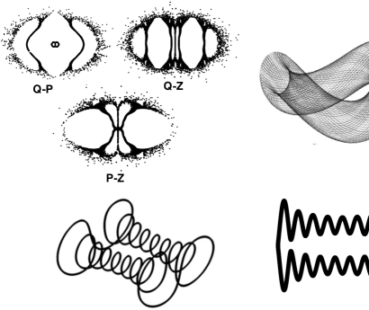
Figure 1: Chaotic and torus solutions of the equilibrium Nosé-Hoover equations:
$\{\ \dot{q}=p\ ;\ \dot{p}=-q-\zeta p\ ;\ \dot{\zeta}\propto p^{2}-1\ \}\$. See Reference 4 for more details.

Consider next the nonequilibrium situation where the imposed temperature field is a function of the oscillator coordinate $q$. We use a simple interpolation between $T(\mp\infty)=1\mp\epsilon$ :

$$T(q)=1+\epsilon\tanh(q)\ .$$

Here $\epsilon$ is the maximum value of the temperature gradient, $(dT/dq)$, which occurs at $q=0$. One would expect the dissipation to cause the oscillator to transfer heat in the direction counter to the gradient. In a dissipative solution, there is a persistent loss of phase volume, $\langle\ \dot{\otimes}\ \rangle<0$. This loss, along with chaos, is the identifying characteristic of a strange attractor with a fractional information dimension.

Accurate solutions of the temperature-dependent motion equations testing this idea of irresistible dissipation (and often verifying it) can be obtained by numerical integration. For sufficiently-large gradients the oscillator typically has a limit cycle in which heat is transferred in the negative $q$ direction. For smaller gradients, the details become messy, with the same sort of intricate Poincaré structures associated with Hamiltonian chaos. At $\epsilon=0.45$ most trajectories collapse to a limit cycle, while at $\epsilon=0.40$ there is a stable torus solution. In addition to these relatively robust structures, holes in the strange-attractor cross sections for $0<\epsilon<0.40$ indicate the locations of the (infinitely-many) quasi-periodic solutions which thread through the chaotic region. Careful work locates the transition linking the chaotic and limit-cycle solutions near $\epsilon=0.4053_{6}$ .

The two-dimensional sections of the three-dimensional flow are dazzling in their complexity. Their analysis yields a hybrid surprise: parts of the nonequilibrium phase space are, as expected, dissipative, with $\langle\ \zeta\ \rangle>0$ ; but other parts, invariant tori, are conservative, with $\langle\ \zeta\ \rangle=0$. We found it puzzling that these tori are not dissipative.

A helpful referee pointed out to us that a very similar coexistence of conservative and dissipative solutions was found in the laser models investigated in Reference 10. A little reflection suggests that a torus mapping into itself must obey Liouville’s Theorem and so cannot shrink. If dissipation were possible it would necessarily cause the tori to shrink, until they reached their limit cycles. On the other hand, by applying a sufficiently large temperature gradient ($\epsilon=0.45$ is large enough), all the tori can be made to disappear. This remarkable feature, where conservative states coexist with dissipative states is possible because the damping is nonlinear with a local rate of contraction given by the mean friction $\langle\ \zeta\ \rangle$. The time-averaged contraction rate $\langle\ \zeta\ \rangle$ is zero on some orbits and positive on others.

Figure 2 shows two invariant tori coexisting with a limit cycle for $\epsilon=0.42$ projected onto the $qp$-plane. The tori are produced using the initial conditions $(q,\ p,\ \zeta)=(-2.3,\ 0,\ 0)$ and $(3.5,\ 0,\ 0)$, and their Lyapunov exponents are $(0,\ 0,\ 0)$. The limit cycle is produced using the initial conditions $(-2.7,\ 0,\ 0)$, and its Lyapunov exponents are $(0,\ -0.0256,\ -0.0788)$. The three objects are interlinked as shown in Figure 2.

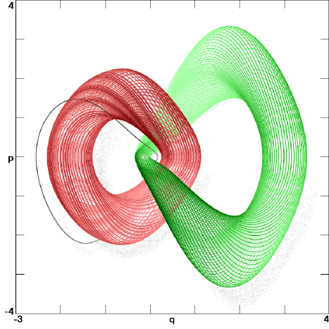
Figure 2: Three interlocked phase-space structures, two conservative “invariant” tori and a dissipative limit cycle, obtained with maximum temperature gradient $\epsilon=0.42$, as described in the text. If time is reversed, with both $p$ and $\zeta$ changing signs, this structural portrait remains unchanged. In the $(q,p,\zeta)$ phase space the temperature is $1+\epsilon\tanh(q)$ .

These tori are only two of an infinite sequence of nested tori as shown in the $\zeta=0$ cross section in Figure 3 where 128 initial conditions are taken uniformly over the interval $-5<q<5$ with $p=\zeta=0$. The cross section of the limit cycle is shown there as two small red dots. The basin boundary of the limit cycle appears to coincide with the outermost torus and extends to infinity in all directions. Orbits starting at points near the basin boundary exhibit transient chaos before eventually converging to the limit cycle.

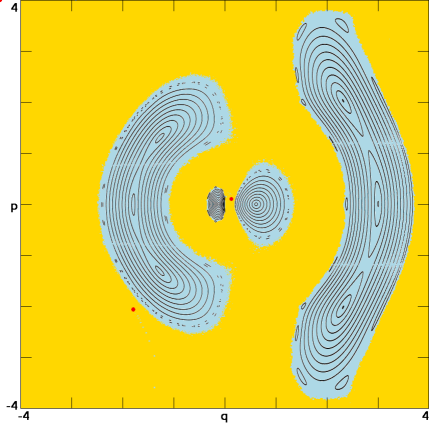
Figure 3: Detailed cross section for $\zeta=0$ of the structure shown in Figure 2 for $\epsilon=0.42$ with 128 initial conditions. The limit cycle is shown in cross section by the two red dots. The dissipative region is shown in maize, the conservative in blue.

Because the system is trapping and invariant under the transformation $p\rightarrow-p,\ \zeta\rightarrow-\zeta,\ t\rightarrow-t$, there is a repelling cycle symmetric with the limit cycle toward which all orbits in the basin of the limit cycle are drawn when time is reversed, while orbits on the tori remain on the tori.

As $\epsilon$ is decreased, the limit cycle loses its stability around $\epsilon=0.4053_{6}$ and becomes a weakly chaotic, nearly space-filling strange attractor while the tori increase in size and complexity. At $\epsilon=0.38$, the Lyapunov exponents in the chaotic region are $(0.0019,\ 0,\ -0.0020)$, and the Kaplan-Yorke dimension is $2.945$. The time-averaged dissipation is tiny as given by $\langle\ \zeta\ \rangle\simeq 1.2\times 10^{-4}$, but decidedly nonzero. This attractor dimension is in sharp contrast to the dimensions of strange attractors like Lorenz’, and Rössler’s. Those three-dimensional flows have fractal dimensions only slightly greater than $2.0$. A cross section of our $(q,\ p,\ \zeta)$ flow with $\epsilon=0.38$ in the $\zeta=0$ plane is shown in Figure 4. What looks like a conservative chaotic sea is actually a weakly dissipative multifractal strange attractor with a capacity dimension of $3.0$ and a correlation dimension of $2.09$. The laser solutions of Reference 10 show similar structures.

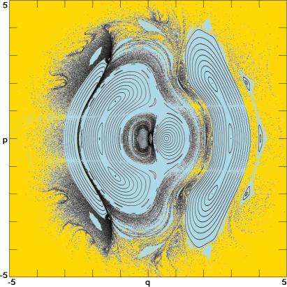
Figure 4: Cross section for $\zeta=0$ using 128 initial conditions ( dissipative in maize and conservative in blue ) as in Figure 3, but with a maximum temperature gradient $\epsilon=0.38$, as described in the text.

As $\epsilon$ is decreased further, the strange attractor becomes more chaotic (its largest Lyapunov exponent increases) while the dissipation decreases until it vanishes at $\epsilon=0$ where the strange attractor becomes a chaotic sea with Lyapunov exponents of $(0.0139,\ 0,\ -0.0139)$. The system is then purely conservative with invariant tori coexisting with the chaotic sea.

The complexity of the single-thermostat oscillator system $(\ q,p,\zeta\ )$ is due to its extreme lack of ergodicity. This property of the model led to attempts to remedy that lackb17 ; b18 ; b19 . Two of these, one fixing both the second and the fourth moments of momentumb17 , and the other fixing the oscillator second moment as well as the second moment of the friction coefficientb19 , are applied to the oscillator problem in the following Section.

IV Robust Heat Transfer with a Harmonic Oscillator

Hoover and Holianb17 used two thermostat control variables, $\zeta$ and $\xi$, fixing both the second and the fourth long-time-averaged moments of momentum, $\langle\ p^{2},p^{4}\ \rangle$ . The four equations of motions, which generate Gibbs’ canonical distribution for a fixed temperature $T$ become:

$$\{\ \dot{q}=p\ ;\ \dot{p}=-q-\zeta p-\xi p^{3}\ ;\ \dot{\zeta}=p^{2}-T\ ;\ \dot{\xi}=p^{4}-3p^{2}T\ \}\ {\rm[\ HH\ ]}\ .$$

Both $\zeta$ and $\xi$ have Gaussian distributionsb17 . These equations of motion are evidently ergodic, according to careful tests carried out by Posch and Hooverb6 . Another isothermal set of four motion equations, due to Martyna, Klein, and Tuckermanb18 , are likewise thought to be ergodic:

$$\{\ \dot{q}=p\ ;\ \dot{p}=-q-\zeta p\ ;\ \dot{\zeta}=p^{2}-T-\xi\zeta\ ;\ \dot{\xi}=\zeta^{2}-T\ \}\ {\rm[\ MKT\ ]}\ .$$

To avoid confusion, but perhaps not controversy, we explain what we mean by “ergodicity”, which we believe to be quite similar to the Ehrenfests’ concept of “quasi-ergodicity”. We choose a generalized (four-dimensional) cube (or parallelepiped, or sphere, or some other compact shape) and ask whether a trajectory started anywhere within this four-dimensional volume will eventually come arbitrarily near any other point in the volume. If so, “ergodic”. If not, not ergodic.

Let us consider next generalized versions of the Hoover-Holian and Martyna-Klein-Tuckerman oscillators with the hyperbolic-tangent temperature field $T=1+\epsilon\tanh(q)$ . First, consider the four-dimensional, time-reversible dynamics of the doubly-thermostated, one-dimensional HH oscillator with a maximum temperature gradient of $\epsilon=0.40$. Figure 5 shows those $(\ q,p\ )$ values close to equilibrium whenever $|\zeta|<0.005$ and $|\xi|<0.005$. This method of obtaining a double cross section has the virtue that the density of points in the two-dimensional plot is proportional to the density in the full $(q,p,\zeta,\xi)$ four-dimensional phase space. Although there is considerable structure in the plot, there is no evidence for the holes common to the three-dimensional system. We believe that the reason for this uniformity is the vanishing likelihood for finding a periodic orbit in the three-dimensional space defining a three-dimensional “Poincaré volume”, analogous to a two-dimensional Poincaré section. Figure 6 is the double cross section view using the MKT chain-thermostat idea of Reference 18 with $\epsilon=0.20$.

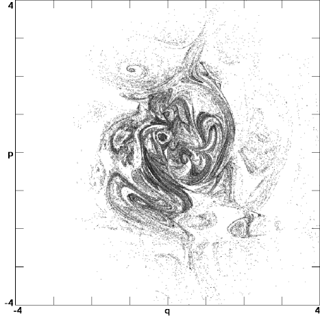
Figure 5: Double cross section ($\zeta=\xi=0$) for the nonequilibrium version of the four HH equations of Reference 17 with $\epsilon=0.40$. The three-dimensional tori are absent here. The Lyapunov exponents are $\{\ 0.0878,\ 0,\ -0.0084,\ -0.1184\ \}$, with capacity dimension 4, Kaplan-Yorke dimension 3.687, and correlation dimension $3.38$.

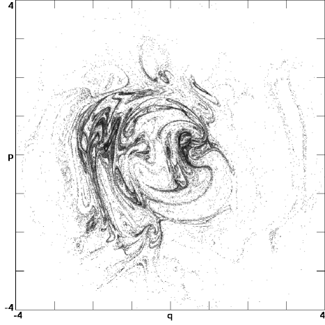
Figure 6: Double cross section ($\zeta=\xi=0$) for the nonequilibrium version of the four MKT equations of Reference 18 with $\epsilon=0.20$. The three-dimensional tori are absent here. The Lyapunov exponents are $\{\ 0.0692,\ 0,\ -0.0159,\ -0.0856\ \}$, with capacity dimension 4, Kaplan-Yorke dimension 3.624, and correlation dimension $3.39$.

Because, for sufficiently small temperature gradients, the HH motion equations from Reference 17 and the MKT motion equations from Reference 18 yield space-filling ergodic solutions, the conventional descriptions in terms of periodic orbits and saddle points are not useful. It appears that perturbing the smoothly continuous Gaussian density,

$$f(q,p,\zeta,\xi)\propto e^{-(q^{2}+p^{2}+\zeta^{2}+\xi^{2})/2}\ ,$$

away from isothermal equilibrium, by adding a further nonlinearity, leads to fractally-concentrated ridges and depleted valleys in the density, much like the perturbations responsible for the earth’s basin and range construction. The formally unanswered question of why the four-dimensional equations are ergodic while the three-dimensional ones are not is important, but we can only provide an informal explanation. We encourage the mathematically-inclined reader to pursue it with vigor and imagination. A simple explanation seems unlikely.

Very recently Patra and Bhattacharya suggested a different thermostating method, fixing both the kinetic and configurational temperatures simultaneously by using two thermostating control variablesb19 . We thank them for several useful emails. Applied to the harmonic oscillator problem, their equations of motion are:

$$\{\ \dot{q}=p-\xi q\ ;\ \dot{p}=-q-\zeta p\ ;\ \dot{\zeta}=p^{2}-T\ ;\ \dot{\xi}=q^{2}-T\ ;\ T\equiv 1+\epsilon\tanh(q)\ \}\ .$$

From the standpoint of control theory the Patra-Bhattacharya thermostating idea is not far from ( a rewritten form of ) the laser equations (2.3) of Politi, Oppo, and Badii :

$$\{\ \dot{q}=p-\zeta q\ ;\ \dot{p}=-q-\zeta p\ ;\ \dot{\zeta}=q^{2}+p^{2}-T\ \}\ .$$

It is interesting to see that the Patra-Bhattacharya set of four equations shows all the complexity of the Nosé-Hoover equations but lacks the space-filling ergodicity of the two other four-dimensional systems investigated here. With $\epsilon=0$ the equilibrium Patra-Bhattacharya equations show a strong correlation between the oscillator coordinate and momentum, with $\langle\ q^{2}p^{2}\ \rangle\simeq 1.41$ rather than unity. Numerical work with these equations is complicated by the fixed points at $\epsilon=0$, $(q,p)=(\pm 1,\pm 1)$ , which can be removed by using other moments.

Sprottb20 has discovered another time-reversible three-dimensional dynamical system which displays coexisting conservative and dissipative regions:

$$\{\ \dot{x}=y+2xy+xz\ ;\ \dot{y}=1-2x^{2}+yz\ ;\ \dot{z}=x-x^{2}-y^{2}\ \}\ .$$

There are now a wealth of such time-reversible dynamical systems which exhibit thermodynamic characteristics.

V Conclusions and Recommendations

A reïnvestigation of the decades-old Nosé-Hoover-Posch-Sprott-Vesely work is well warranted by the more-recent advances in processor speeds. The calculations described here can be carried out on a laptop computer in a clock time measured in a few minutes or hours. In 1984 such problems required multi-million-dollar Cray Supercomputers.

The simplest of the Nosé-Hoover nonequilibrium simulations show a qualitative difference between tori and limit cycles. Only the limit cycles can support dissipation. This dissipation is shared with the space-filling strange attractor that surrounds the various quasi-periodic solutions of the motion equations. How do the tori resist dissipation? A clear explanation is still lacking.

The difference between the complexity of the three-dimensional systems and the relative simplicity of two of the four-dimensional ones (but not the Patra-Bhattacharya equations) is striking. This observation suggests that quasi-periodic structures are relatively rare in four-equation two-or-three-dimensional Poincaré cross sections. On the other hand quasi-periodic structures are commonplace in three-equation two-dimensional Poincaré cross sections. Quasi-periodic solutions are inevitable in two dimensions. The question remains as to why the Patra-Bhattacharya oscillator shows quasi-periodic toroidal behavior for even the smallest values of $\epsilon$.

These results should provide grist for the mathematicians’ mills for some time. We also recommend them to students for further rewarding study.

VI Acknowledgment

We thank Antonio Politi, Karl Travis, and the referees for their suggestions and careful readings of the manuscript. One referee asked that we include the clarifying explanation that “homoclinic cycles partition the phase space into its conservative and dissipative parts, though the relevance of such cycles to macroscopic thermodynamics is still unexplored”.

References

- (1) S. Nosé, “A Molecular Dynamics Method for Simulations in the Canonical Ensemble”, Molecular Physics 52, 255-268 (1984).
- (2) S. Nosé, “A Unified Formulation of the Constant Temperature Molecular Dynamics Methods”, Journal of Chemical Physics 81, 511-519 (1984).
- (3) W. G. Hoover, “Canonical Dynamics: Equilibrium Phase-Space Distributions”, Physical Review A 31, 1695-1697 (1985).
- (4) H. A. Posch, W. G. Hoover, and F. J. Vesely, “Canonical Dynamics of the Nosé Oscillator: Stability, Order, and Chaos”, Physical Review A 33, 4253-4265 (1986).
- (5) H. Bosetti, H. A. Posch, Ch. Dellago, and Wm. G. Hoover, “Time-Reversal Symmetry and Covariant Lyapunov Vectors for Simple Particle Models In and Out of Thermal Equilibrium”, Physical Review E 82, 046218 (2010).
- (6) H. A. Posch and Wm. G. Hoover, “Time-Reversible Dissipative Attractors in Three and Four Phase-Space Dimensions”, Physical Review E 55, 6803-6810 (1997).
- (7) B. L. Holian, W. G. Hoover, and H. A. Posch, “Resolution of Loschmidt’s Paradox: the Origin of Irreversible Behavior in Reversible Atomistic Dynamics”, Physical Review Letters 59, 10-13 (1987).
- (8) J. C. Sprott, “Some Simple Chaotic Flows”, Physical Review E 50, R647-R650 (1994).
- (9) Wm. G. Hoover, “Remark on ‘Some Simple Chaotic Flows’ ”, Physical Review E 51, 759-760 (1995).
- (10) A. Politi, G. L. Oppo, and R. Badii, “Coexistence of Conservative and Dissipative Behavior in Reversible Dynamical Systems”, Physical Review A 33, 4055-4060 (1986).
- (11) Wm. G. Hoover, C. G. Hoover, H. A. Posch, and J. A. Codelli, “The Second Law of Thermodynamics and MultiFractal Distribution Functions: Bin Counting, Pair Correlations, and the [ definite failure of the ] Kaplan-Yorke Conjecture”, Communications in Nonlinear Science and Numerical Simulation 12, 214-231 (2007).
- (12) Wm. G. Hoover and C. G. Hoover, “Why Instantaneous Values of the ‘Covariant’ Lyapunov Exponents Depend upon the Chosen State-Space Scale”, Communications in Nonlinear Science and Numerical Simulation 20, 5-8 (2014).
- (13) D. Kusnezov, A. Bulgac, and W. Bauer, “Canonical Ensembles from Chaos”, Annals of Physics 204, 155-185 (1990) and 214, 180-218 (1992).
- (14) Wm. G. Hoover, “ Mécanique de Nonéquilibre à la Californienne”, Physica 240, 1-11 (1997).
- (15) C. P. Dettmann and G. P. Morriss, “Hamiltonian Reformulation and Pairing of Lyapunov Exponents for Nosé-Hoover Dynamics”, Physical Review E 55, 3693-3696 (1997).
- (16) Wm. G. Hoover and C. G. Hoover, “Hamiltonian Dynamics of Thermostated Systems: Two-Temperature Heat-Conducting Chains”, Journal of Chemical Physics 126, 164113 (2007).
- (17) Wm. G. Hoover and B. L. Holian, “Kinetic Moments Method for the Canonical Ensemble Distribution”, Physics Letters A 211, 253-257 (1996).
- (18) C. J. Martyna, M. L. Klein, and M. Tuckerman, “Nosé-Hoover Chains –the Canonical Ensemble via Continuous Dynamics”, Journal of Chemical Physics 97, 2635-2643 (1992).
- (19) P. K. Patra and B. Bhattacharya, “A Deterministic Thermostat for Controlling Temperature using All Degrees of Freedom”, Journal of Chemical Physics 140, 064106 (2014).
- (20) J. C. Sprott, “A Dynamical System with a Strange Attractor and Invariant Tori”, Physics Letters A 378, 1361-1363 (2014).