Order, chaos and quasi symmetries in
a first-order quantum phase transition

Abstract

We study the competing order and chaos in a first-order quantum phase transition with a high barrier. The boson model Hamiltonian employed, interpolates between its U(5) (spherical) and SU(3) (deformed) limits. A classical analysis reveals regular (chaotic) dynamics at low (higher) energy in the spherical region, coexisting with a robustly regular dynamics in the deformed region. A quantum analysis discloses, amidst a complicated environment, persisting regular multiplets of states associated with partial U(5) and quasi SU(3) dynamical symmetries.

1 Introduction

Quantum phase transitions (QPTs) are qualitative changes in the ground state properties of a physical system induced by a variation of parameters $\lambda$ in the quantum Hamiltonian $\hat{H}(\lambda)$ [1, 2]. Such ground-state transformations have received considerable attention in recent years and have found a variety of applications in many areas of physics and chemistry [3]. The particular type of QPT is reflected in the topology of the underlying mean-field (Landau) potential $V(\lambda)$. Most studies have focused on second-order (continuous) QPTs [4], where $V(\lambda)$ has a single minimum which evolves continuously into another minimum. The situation is more complex for discontinuous (first-order) QPTs, where $V(\lambda)$ develops multiple minima that coexist in a range of $\lambda$ values and cross at the critical point, $\lambda\!=\!\lambda_{c}$. The interest in such QPTs stems from their key role in phase-coexistence phenomena at zero temperature. Examples are offered by the metal-insulator Mott transition [5], heavy-fermion superconductors [6], quantum Hall bilayers [7] and shape-coexistence in mesoscopic systems, such as atomic nuclei [8].

The competing interactions in the Hamiltonian that drive these ground-state phase transitions can affect dramatically the nature of the dynamics and, in some cases, lead to the emergence of quantum chaos. This effect has been observed in quantum optics models of $N$ two-level atoms interacting with a single-mode radiation field [9], where the onset of chaos is triggered by continuous QPTs. In the present contribution, we address the mixed regular and chaotic dynamics associated with a first order QPT [10, 11, 12]. For that purpose, we employ an interacting boson model which describes such QPTs between spherical and axially-deformed nuclei. The model is amenable to both classical and quantum treatments, has a rich group structure and inherent geometry, which makes it an ideal framework for studying the intricate interplay of order and chaos and the role of symmetries in such shape-phase transitions.

2 Symmetries, geometry and quantum phase transitions in the IBM

The interacting boson model (IBM) [13] describes low-lying quadrupole collective states in nuclei in terms of $N$ interacting monopole $(s)$ and quadrupole $(d)$ bosons representing valence nucleon pairs. The bilinear combinations ${\cal G}_{ij}\equiv b^{{\dagger}}_{i}b_{j}=\{s^{{\dagger}}s,\,s^{{\dagger}}d_{m},\,d^{{\dagger}}_{m}s,\,d^{{\dagger}}_{m}d_{m^{\prime}}\}$ span a U(6) algebra, which serves as the spectrum generating algebra. The IBM Hamiltonian is expanded in terms of these generators, $\hat{H}=\sum_{ij}\epsilon_{ij}\,{\cal G}_{ij}+\sum_{ijk\ell}u_{ijk\ell}\,{\cal G}_{ij}{\cal G}_{k\ell}$, and consists of Hermitian, rotational-invariant interactions which conserve the total number of $s$- and $d$- bosons, $\hat{N}=\hat{n}_{s}+\hat{n}_{d}=s^{\dagger}s+\sum_{m}d^{\dagger}_{m}d_{m}$. A dynamical symmetry (DS) occurs if the Hamiltonian can be written in terms of the Casimir operators of a chain of nested sub-algebras of U(6). The Hamiltonian is then completely solvable in the basis associated with each chain. The three dynamical symmetries of the IBM and corresponding bases are

$${\rm U(6)}\supset{\rm U(5)}\supset{\rm O(5)}\supset{\rm O(3)}\qquad|N,n_{d},\tau,n_{\Delta},L\rangle\;\;\;\;\,\;{\rm spherical\;vibrator}$$ (1a)

$${\rm U(6)}\supset{\rm SU(3)}\supset{\rm O(3)}\qquad\qquad\;\;\,|N,(\lambda,\mu),K,L\rangle\quad\;\;{\rm axially}{\rm-deformed\;rotor}$$ (1b)

$${\rm U(6)}\supset{\rm O(6)}\supset{\rm O(5)}\supset{\rm O(3)}\qquad|N,\sigma,\tau,n_{\Delta},L\rangle\qquad\,\gamma{\rm-unstable\;deformed\;rotor}\qquad\quad$$ (1c)

The associated analytic solutions resemble known limits of the geometric model of nuclei [14], as indicated above. The basis members are classified by the irreducible representations (irreps) of the corresponding algebras. Specifically, the quantum numbers $N,n_{d},(\lambda,\mu),\sigma,\tau$ and $L$ label the relevant irreps of ${\rm U(6),U(5),SU(3),O(6),O(5)}$ and ${\rm O(3)}$, respectively. $n_{\Delta}$ and $K$ are multiplicity labels needed for complete classification in the reductions ${\rm O(5)}\supset{\rm O(3)}$ and ${\rm SU(3)}\supset{\rm O(3)}$, respectively. Each basis is complete and can be used for a numerical diagonalization of the Hamiltonian in the general case. A geometric visualization of the model is obtained by a potential surface, $V(\beta,\gamma)\!=\!\langle\beta,\gamma;N|\hat{H}|\beta,\gamma;N\rangle$, defined by the expectation value of the Hamiltonian in the intrinsic condensate state [15, 16]

$$|\beta,\gamma;N\rangle = (N!)^{-1/2}[\,\Gamma^{\dagger}_{c}(\beta,\gamma)\,]^{N}|0\rangle~{},$$ (2a)

$$\Gamma^{\dagger}_{c}(\beta,\gamma) = \left[\beta\cos\gamma d^{\dagger}_{0}+\beta\sin{\gamma}(d^{\dagger}_{2}+d^{\dagger}_{-2})/\sqrt{2}+\sqrt{2-\beta^{2}}s^{\dagger}\right]/\sqrt{2}~{}.$$ (2b)

Here $(\beta,\gamma)$ are quadrupole shape parameters analogous to the variables of the collective model of nuclei. Their values $(\beta_{\mathrm{eq}},\gamma_{\mathrm{eq}})$ at the global minimum of $V(\beta,\gamma)$ define the equilibrium shape for a given Hamiltonian. For one- and two-body interactions, the shape can be spherical $(\beta_{\mathrm{eq}}=0)$ or deformed $(\beta_{\mathrm{eq}}>0)$ with $\gamma_{\mathrm{eq}}=0$ (prolate), $\gamma_{\mathrm{eq}}=\pi/3$ (oblate), or $\gamma$-independent.

The dynamical symmetries of Eq. (1), correspond to phases of the system, and provide analytic benchmarks for the dynamics of stable nuclear shapes. Quantum phase transitions (QPTs) between such stable shapes have been studied extensively in the IBM framework [16, 17] and are manifested empirically in nuclei [8]. The Hamiltonians employed mix interaction terms from different DS chains, e.g., $\hat{H}(\lambda)=\lambda\hat{H}_{a}+(1-\lambda)\hat{H}_{b}$. The coupling coefficient $(\lambda$) responsible for the mixing, serves as the control parameter and the surface, $V(\lambda)\equiv V(\lambda;\beta,\gamma)$, serves as the Landau potential. In general, under such circumstances, solvability is lost, there are no remaining non-trivial conserved quantum numbers and all eigenstates are expected to be mixed. However, for particular symmetry breaking, some intermediate symmetry structure can survive. The latter include partial dynamical symmetry (PDS) [18] and quasi-dynamical symmetry (QDS) [19]. In a PDS, the conditions of an exact dynamical symmetry (solvability of the complete spectrum and existence of exact quantum numbers for all eigenstates) are relaxed and apply to only part of the eigenstates. In a QDS, particular states continue to exhibit selected characteristic properties (e.g., energy and B(E2) ratios) of the closest dynamical symmetry, in the face of strong-symmetry breaking interactions. This “apparent” symmetry is due to the coherent nature of the mixing. As discussed below, both PDS and QDS are relevant to quantum phase transitions [19, 20].

In view of the central role of the Landau potential, $V(\beta,\gamma)$, for QPTs, it is convenient to resolve the Hamiltonian into two parts, $\hat{H}=\hat{H}_{\mathrm{int}}+\hat{H}_{\mathrm{col}}$ [21]. The intrinsic part ($\hat{H}_{\mathrm{int}}$) determines the potential surface while the collective part ($\hat{H}_{\mathrm{col}}$) is composed of kinetic terms which do not affect the shape of $V(\beta,\gamma)$. For first-order QPTs, the resolution allows the construction of an intrinsic Hamiltonian with a high-barrier [22], and by treating it separately, one avoids the complication of rotation-vibration couplings that can obscure the simple pattern of mixed dynamics, reported below. Henceforth, we confine the discussion to the dynamics of the intrinsic Hamiltonian.

3 Intrinsic Hamiltonian for a first-order QPT

Focusing on first-order QPTs between stable spherical ($\beta_{\mathrm{eq}}=0$) and prolate-deformed ($\beta_{\mathrm{eq}}>0$, $\gamma_{\mathrm{eq}}=0$) shapes, the intrinsic Hamiltonian reads

$$\hat{H}_{1}(\rho)/\bar{h}_{2} = 2(1\!-\!2\rho^{2})\hat{n}_{d}(\hat{n}_{d}\!-\!1)+2R^{{\dagger}}_{2}(\rho)\cdot\tilde{R}_{2}(\rho)~{},$$ (3a)

$$\hat{H}_{2}(\xi)/\bar{h}_{2} = \xi P^{{\dagger}}_{0}P_{0}+P^{{\dagger}}_{2}\cdot\tilde{P}_{2}~{},$$ (3b)

where $\hat{n}_{d}$ is the $d$-boson number operator, $R^{{\dagger}}_{2\mu}(\rho)\!=\!\sqrt{2}s^{\dagger}d^{\dagger}_{\mu}+\rho\sqrt{7}(d^{\dagger}d^{\dagger})^{(2)}_{\mu}$, $P^{{\dagger}}_{0}\!=\!d^{\dagger}\cdot d^{\dagger}-2(s^{\dagger})^{2}$ and $P^{{\dagger}}_{2\mu}\!=\!2s^{\dagger}d^{\dagger}_{\mu}+\sqrt{7}(d^{\dagger}d^{\dagger})^{(2)}_{\mu}$. Here $\tilde{R}_{2\mu}\!=\!(-1)^{\mu}R_{2,-\mu}$, $\tilde{P}_{2\mu}\!=\!(-1)^{\mu}P_{2,-\mu}$ and the dot implies a scalar product. Scaling by $\overline{h}_{2}\equiv h_{2}/N(N-1)$ is used throughout, to facilitate the comparison with the classical limit. The control parameters that drive the QPT are $\rho$ and $\xi$, with $0\leq\rho\leq\tfrac{1}{\sqrt{2}}$ and $0\leq\xi\leq 1$.

The intrinsic Hamiltonian in the spherical phase, $\hat{H}_{1}(\rho)$, has by construction the intrinsic state of Eq. (2) with $\beta_{\mathrm{eq}}\!=\!0$ as zero energy eigenstate. For large $N$, its normal modes involve quadrupole vibrations about the spherical global minimum of the potential surface, with frequency $\epsilon\!=\!4\bar{h}_{2}N$. For $\rho=0$ it reduces to

$$\hat{H}_{1}(\rho=0)/\bar{h}_{2} = 2\hat{n}_{d}(\hat{n}_{d}-1)+4(\hat{N}-\hat{n}_{d})\hat{n}_{d}~{}.$$ (4)

Since $\hat{n}_{d}$ is the linear Casimir operator of U(5), $\hat{H}_{1}(\rho=0)$ has U(5) dynamical symmetry (DS). The spectrum is completely solvable $E_{\rm DS}=[2n_{d}(n_{d}-1)+4(N-n_{d})n_{d}]\bar{h}_{2}$, and the eigenstates, $|N,n_{d},\tau,n_{\Delta},L\rangle$, are those of the U(5) chain, Eq. (1a). The spectrum resembles that of an anharmonic spherical vibrator, describing quadrupole excitations of a spherical equilibrium shape. The lowest U(5) multiplets involve states with quantum numbers $(n_{d}\!=\!0,\tau\!=\!0,L\!=\!0)$, $(n_{d}\!=\!1,\tau\!=\!1,L\!=\!2)$, $(n_{d}\!=\!2,\tau\!=\!2,L\!=\!2,4;\tau=0,L=0)$, $(n_{d}\!=\!3,\tau\!=\!3,L\!=\!6,4,3,0;\tau\!=\!1,L\!=\!2)$.

For $\rho>0$, $\hat{H}_{1}(\rho)$ has an additional $\rho[(d^{{\dagger}}d^{{\dagger}})^{(2)}\cdot\tilde{d}s+s^{{\dagger}}d^{{\dagger}}\cdot(\tilde{d}\tilde{d})^{(2)}]$ term, which breaks the U(5) DS, and induces U(5) and O(5) mixing subject to $\Delta n_{d}=\pm 1$ and $\Delta\tau=\pm 1,\pm 3$. The explicit breaking of O(5) symmetry leads to non-integrability and, as will be shown in subsequent discussions, is the main cause for the onset of chaos in the spherical region. Although $\hat{H}_{1}(\rho>0)$ is not diagonal in the U(5) chain, it retains the following selected solvable U(5) basis states

$$|N,n_{d}=\tau=L=0\rangle\;\;\;\; E_{\rm PDS}=0~{},$$ (5a)

$$|N,n_{d}=\tau=L=3\rangle\;\;\;\; E_{\rm PDS}=12\left(N-2+3\rho^{2}\right)\bar{h}_{2}~{},$$ (5b)

while other eigenstates are mixed with respect to U(5). As such, it exhibits U(5) partial dynamical symmetry [U(5)-PDS].

The intrinsic Hamiltonian in the deformed phase, $\hat{H}_{2}(\xi)$, has by construction the intrinsic state of Eq. (2) $|\beta_{\mathrm{eq}}=\tfrac{2}{\sqrt{3}},\gamma_{\mathrm{eq}}=0;N\rangle$ as zero energy eigenstate. For large $N$, its normal modes involve both $\beta$ and $\gamma$ vibrations about the deformed global minimum of $V(\beta,\gamma)$, with frequencies $\epsilon_{\beta}\!=\!4\bar{h}_{2}N(2\xi+1)$ and $\epsilon_{\gamma}\!=\!12\bar{h}_{2}N$. For $\xi=1$, the Hamiltonian reduces to

$$\hat{H}_{2}(\xi=1)/\bar{h}_{2} = -\hat{C}_{\rm SU(3)}+2\hat{N}(2\hat{N}+3)~{},$$ (6)

It involves the quadratic Casimir of SU(3) and hence has SU(3) DS. The spectrum is completely solvable, $E_{\rm DS}/\bar{h}_{2}=[-(\lambda^{2}+\mu^{2}+\lambda\mu+3\lambda+3\mu)+2N(2N+3)]\bar{h}_{2}$, and the eigenstates, $|N,(\lambda,\mu),K,L\rangle$, are those of the SU(3) chain , Eq. (1b). The spectrum resembles that of an axially-deformed rotor with degenerate $K$-bands arranged in SU(3) $(\lambda,\mu)$ multiplets, $K$ being the angular momentum projection on the symmetry axis. The rotational states in each band have angular momenta $L=0,\,2,\,4\ldots$, for $K=0$ and $L=K,K+1,K+2,\ldots$, for $K>0$. The lowest SU(3) multiplets are $(2N,0)$ which contains the ground band $g(K=0)$, and $(2N-4,2)$ which contains the $\beta(K=0)$ and $\gamma(K=2)$ bands.

For $\xi<1$, $\hat{H}_{2}(\xi)$ has an additional term, $(\xi-1)P^{{\dagger}}_{0}P_{0}$, which breaks the SU(3) DS and most eigenstates are mixed with respect to SU(3). However, the following states

$$|N,(2N,0)K=0,L\rangle\;\;\;\;L=0,2,4,\ldots,2N$$

$$E_{\rm PDS}=0$$ (7a)

$$|N,(2N-4k,2k)K=2k,L\rangle\;\;\;\;L=K,K+1,\ldots,(2N-2k)\qquad\;k>0~{},\qquad\qquad$$

$$E_{\rm PDS}=6k\left(2N-2k+1\right)\bar{h}_{2}$$ (7b)

remain solvable with good SU3) symmetry. As such, $\hat{H}_{2}(\xi<1)$ exhibits SU(3) partial dynamical symmetry [SU(3)-PDS]. The selected states of Eq. (7) span the ground band $g(K=0)$ and $\gamma^{k}(K=2k)$ bands.

The intrinsic Hamiltonians, $\hat{H}_{1}(\rho)$ and $\hat{H}_{2}(\xi)$ of Eq. (3), with $0\leq\rho\leq\tfrac{1}{\sqrt{2}}$ and $0\leq\xi\leq 1$, interpolate between the U(5) $(\rho\!=\!0)$ and SU(3) $(\xi\!=\!1)$ DS limits. The two Hamiltonians coincide at the critical point $\rho_{c}\!=\!\tfrac{1}{\sqrt{2}}$ and $\xi_{c}\!=\!0$: $\hat{H}_{1}(\rho_{c})=\hat{H}_{2}(\xi_{c})$. Both Hamiltonians support subsets of solvable PDS states, Eqs. (5) and (7), whose analytic properties provide unique signatures for their identification in the quantum spectrum.

4 Classical limit and topology of the Landau potential

The classical limit of the IBM is obtained through the use of Glauber coherent states. This amounts to replacing $(s^{\dagger},\,d^{\dagger}_{\mu})$ by six c-numbers $(\alpha_{s}^{*},\,\alpha_{\mu}^{*})$ rescaled by $\sqrt{N}$ and taking $N\rightarrow\infty$, with $1/N$ playing the role of $\hbar$ [23]. Number conservation ensures that phase space is 10-dimensional and can be phrased in terms of two shape (deformation) variables, three orientation (Euler) angles and their conjugate momenta. The shape variables can be identified with the $\beta,\gamma$ variables introduced through Eq. (2). Setting all momenta to zero, yields the classical potential which is identical to $V(\beta,\gamma)$ mentioned above. In the classical analysis presented below we consider, for simplicity, the dynamics of $L=0$ vibrations, for which only two degrees of freedom are active. The rotational dynamics with $L>0$ is examined in the subsequent quantum analysis.

For the intrinsic Hamiltonian of Eq. (3), constrained to $L=0$, the above procedure yields the following classical Hamiltonian

$$\mathcal{H}_{1}(\rho)/h_{2} = {\cal H}_{d,0}^{2}+2(1-{\cal H}_{d,0}){\cal H}_{d,0}+2\rho^{2}p_{\gamma}^{2}$$ (8a)

$$+\rho\sqrt{2(1-{\cal H}_{d,0})}\left[\,(p_{\gamma}^{2}/\beta-\beta p^{2}_{\beta}-\beta^{3})\cos{3\gamma}+2p_{\beta}p_{\gamma}\sin{3\gamma}\,\right]~{},$$

$$\mathcal{H}_{2}(\xi)/h_{2} = {\cal H}_{d,0}^{2}+2(1\!\!-\!\!{\cal H}_{d,0}){\cal H}_{d,0}+p_{\gamma}^{2}$$ (8b)

$$+\sqrt{1-{\cal H}_{d,0}}\left[\,(p_{\gamma}^{2}/\beta-\beta p^{2}_{\beta}-\beta^{3})\cos{3\gamma}+2p_{\beta}p_{\gamma}\sin{3\gamma}\,\right]\qquad$$

$$+\xi\left[\,\beta^{2}p_{\beta}^{2}+\tfrac{1}{4}(\beta^{2}-T)^{2}-2(1-{\cal H}_{d,0})(\beta^{2}-T)+4(1\!\!-\!\!{\cal H}_{d,0})^{2}\,\right]~{}.$$

Here the coordinates $\beta\in[0,\sqrt{2}]$, $\gamma\in[0,2\pi)$ and their canonically conjugate momenta $p_{\beta}\in[0,\sqrt{2}]$ and $p_{\gamma}\in[0,1]$ span a compact classical phase space. The term, ${\cal H}_{d,0}=(T+\beta^{2})/2$ with $T=p_{\beta}^{2}+p_{\gamma}^{2}/\beta^{2}$, denotes the classical limit of $\hat{n}_{d}$ (restricted to $L=0$) and forms an isotropic harmonic oscillator Hamiltonian in the $\beta$ and $\gamma$ variables. Notice that the classical Hamiltonian of Eq. (8) contains complicated momentum-dependent terms originating from the two-body interactions in the Hamiltonian (3), not just the usual quadratic kinetic energy $T$. Setting $p_{\beta}=p_{\gamma}=0$ in Eq. (8) leads to the following classical potential

$$V_{1}(\rho)/h_{2} = 2\beta^{2}-2\rho\sqrt{2\!-\!\beta^{2}}\beta^{3}\cos 3\gamma-\textstyle{\frac{1}{2}}\beta^{4}~{},$$ (9a)

$$V_{2}(\xi)/h_{2} = 2(1-3\xi)\beta^{2}-\sqrt{2(2\!-\!\beta^{2})}\beta^{3}\cos 3\gamma+\textstyle{\frac{1}{4}}(9\xi-2)\beta^{4}+4\xi~{}.$$ (9b)

The variables $\beta$ and $\gamma$ can be interpreted as polar coordinates in an abstract plane parametrized by Cartesian coordinates $x\!=\!\beta\cos{\gamma}$ and $y\!=\!\beta\sin{\gamma}$. Using these relations together with $p_{x}\!=\!p_{\beta}\cos\gamma-(p_{\gamma}/\beta)\sin\gamma$ and $p_{y}\!=\!(p_{\gamma}/\beta)\cos\gamma+p_{\beta}\sin\gamma$, one can cast the classical Hamiltonian, Eq. (8) and potential, Eq. (9), in Cartesian form. Thus, ${\cal H}_{d,0}=(p_{x}^{2}+p_{y}^{2}+x^{2}+y^{2})/2$ and the potentials $V(\beta,\gamma)=V(x,y)$ depend on the combinations $\beta^{2}\!=\!x^{2}+y^{2}$, $\beta^{4}=(x^{2}+y^{2})^{2}$ and $\beta^{3}\cos 3\gamma\!=\!x^{3}-3xy^{2}$.

The control parameters $\rho$ and $\xi$ determine the landscape and extremal points of the potentials $V_{1}(\rho;\beta,\gamma)$ and $V_{2}(\xi;\beta,\gamma)$, Eq. (9). Important values of these parameters at which a pronounced change in structure is observed, are the spinodal point $(\rho^{*})$ where a second (deformed) minimum occurs, an anti-spinodal point $(\xi^{**})$ where the first (spherical) minimum disappears and a critical point $(\rho_{c},\xi_{c})$ in-between, where the two minima are degenerate. For the potentials under discussion, the values of the control parameters at these points are

$$\rho^{*}=\tfrac{1}{2}\;\;\;,\;\;\;(\rho_{c}=\tfrac{1}{\sqrt{2}}\,,\,\xi_{c}=0)\;\;\;,\;\;\;\xi^{**}=\tfrac{1}{3}\;\;\;.$$ (10)

The critical point separates the spherical and deformed phases. The spinodal and anti-spinodal points embrace it and mark the boundary of the phase coexistence region.

In general, the only $\gamma$-dependence in the potentials (9) is due to the $\sqrt{2-\beta^{2}}\beta^{3}\cos 3\gamma$ term. This induces a three-fold symmetry about the origin $\beta\!=\!0$. As a consequence, the deformed extremal points are obtained for $\gamma\!=\!0,\tfrac{2\pi}{3},\tfrac{4\pi}{3}$ (prolate shapes), or $\gamma\!=\!\tfrac{\pi}{3},\textstyle{\pi},\tfrac{5\pi}{3}$ (oblate shapes). It is therefore possible to restrict the analysis to $\gamma=0$ and allow for both positive and negative values of $\beta$, corresponding to prolate and oblate deformations, respectively. The potentials $V(\beta,\gamma=0)\!=\!V(x,y=0)$ for several values of $\xi,\rho$, are shown at the bottom rows of Figs. 2-4.

The relevant potential in the spherical phase is $V_{1}(\rho;\beta,\gamma)$, Eq. (9a), with $0\leq\rho\leq\rho_{c}$. In this case, $\beta_{\rm eq}=0$ is a global minimum of the potential at an energy $V_{\rm sph}=0$, representing the spherical equilibrium shape. The limiting value at the domain boundary is $V_{\rm lim}=V_{1}(\rho;\beta=\sqrt{2},\gamma)=2h_{2}$. For $\rho=0$, (the U(5) limit), the potential is independent of $\gamma$ and has $\beta_{\rm eq}=0$ as a single minimum. For $\rho>0$, the potential depends on $\gamma$, and $\beta=0$ remains a single minimum for $0\leq\rho<\rho^{*}$, At the spinodal point $\rho^{*}$, $V_{1}(\rho)$ acquires an additional deformed local minimum at an energy $V_{\rm def}>0$, and a barrier develops between the two minima. The spherical and deformed minima cross and become degenerate at the critical point $(\rho_{c},\xi_{c})$.

The relevant potential in the deformed phase is $V_{2}(\xi;\beta,\gamma)$, Eq. (9b), with $\xi\geq\xi_{c}$. In this case, $[\beta_{\rm eq}=\tfrac{2}{\sqrt{3}},\gamma_{\rm eq}=0]$ is a global minimum of the potential at an energy $V_{\rm def}=0$, representing the deformed equilibrium shape. The limiting value of the domain boundary is $V_{\rm lim}=V_{2}(\xi;\beta=\sqrt{2},\gamma)=(2+\xi)h_{2}$. The two potentials coincide at the critical point $(\rho_{c},\xi_{c})$, $V_{2}(\xi_{c};\beta,\gamma)=V_{1}(\rho_{c};\beta,\gamma)$, and the barrier height is $V_{\rm bar}\!=\!\frac{1}{2}h_{2}(1-\sqrt{3})^{2}=0.268h_{2}$. The spherical minimum turns local in $V_{2}(\xi)$ for $\xi>\xi_{c}$ with energy $V_{\rm sph}=4h_{2}\xi>0$, and disappears at the anti-spinodal point $\xi^{**}$. For $\xi>\xi^{**}$, $\beta=0$ turns into a maximum and the potential remains with a single deformed minimum, reaching the SU(3) limit at $\xi=1$.

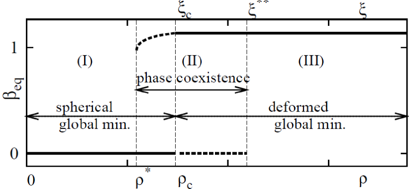
Figure 1: Behavior of the order parameter, $\beta_{\mathrm{eq}}$, as a function of the control parameters ($\rho,\xi$) of the intrinsic Hamiltonian, Eq. (3). Here $\rho^{*},\,(\rho_{c},\,\xi_{c}),\,\xi^{**}$, are the spinodal, critical and anti-spinodal points, respectively, with values given in Eq. (10). The deformation at the global (local) minimum of the Landau potential (9) is marked by solid (dashed) lines. $\beta_{\mathrm{eq}}\!=\!0$ ($\beta_{\mathrm{eq}}\!=\tfrac{2}{\sqrt{3}}$) on the spherical (deformed) side of the QPT. Region I (III) involves a single spherical (deformed) shape, while region II involves shape-coexistence.

The indicated changes in the topology of the potential surfaces upon variation of the control parameters $(\rho,\xi)$, identify three regions with distinct structure.

1. The region of a stable spherical phase, $\rho\in[0,\rho^{*}]$, where the potential has a single spherical minimum.

2. The region of phase coexistence, $\rho\in(\rho^{*},\rho_{c}]$ and $\xi\in[\xi_{c},\xi^{**})$, where the potential has both spherical and deformed minima which cross and become degenerate at the critical point.

3. The region of a stable deformed phase, $\xi>\xi^{**}$, where the potential has a single deformed minimum.

The potential surface in each region serves as the Landau potential of the QPT, with the equilibrium deformations as order parameters. The latter evolve as a function of the control parameters ($\rho,\xi$) and exhibit a discontinuity typical of a first order transition. As depicted in Fig 1, the order parameter ${\beta_{\mathrm{e}q}}$ is a double-valued function in the coexistence region (in-between $\rho^{*}$ and $\xi^{**}$) and a step-function outside it. In what follows, we examine the nature of the classical and quantum dynamics in each region.

5 Classical analysis

Chaotic properties of the IBM have been studied extensively [24], albeit, with a simplified Hamiltonian, giving rise to an extremely low barrier. A new element in the present study is the presence of a high barrier at the critical-point, $V_{\rm bar}/h_{2}\!=\!0.268$, compared to $V_{\rm bar}/h_{2}\!=\!0.0018$ in previous works. This allows the uncovering of a rich pattern of regularity and chaos across a generic first-order QPT in a wide coexistence region.

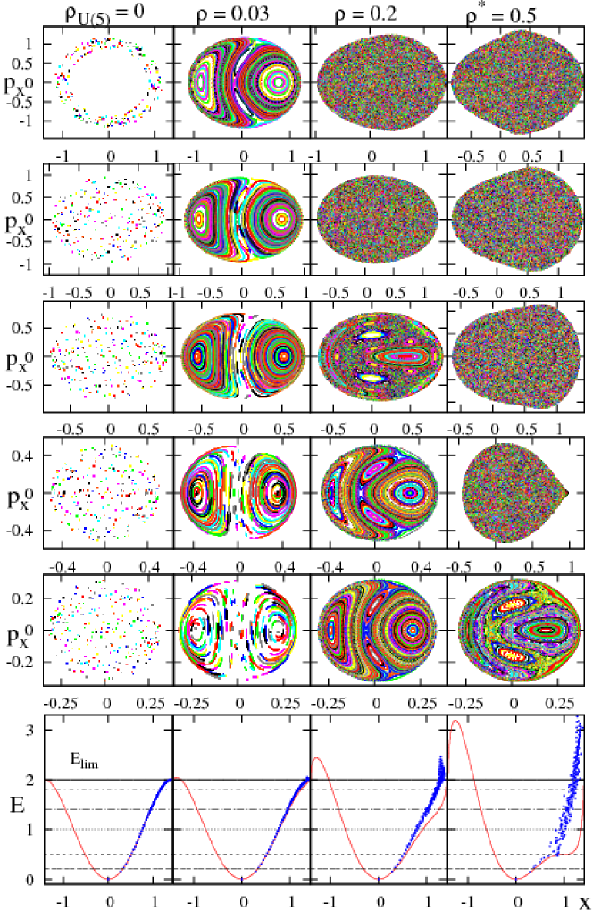
Figure 2: Poincaré sections in the stable spherical phase (region I). Upper five rows depict the classical dynamics of ${\cal H}_{1}(\rho)$ (8a) with $h_{2}=1$, for several values of $\rho\leq\rho^{**}$. The bottom row displays the Peres lattices $\{x_{i},E_{i}\}$, portraying the quantum dynamics for $(N=80,L=0)$ eigenstates of $\hat{H}_{1}(\rho)$ (3a), overlayed on the classical potentials $V_{1}(\rho;x,y=0)$ (9a). The five energies at which the sections were calculated consecutively, are indicated by horizontal lines.

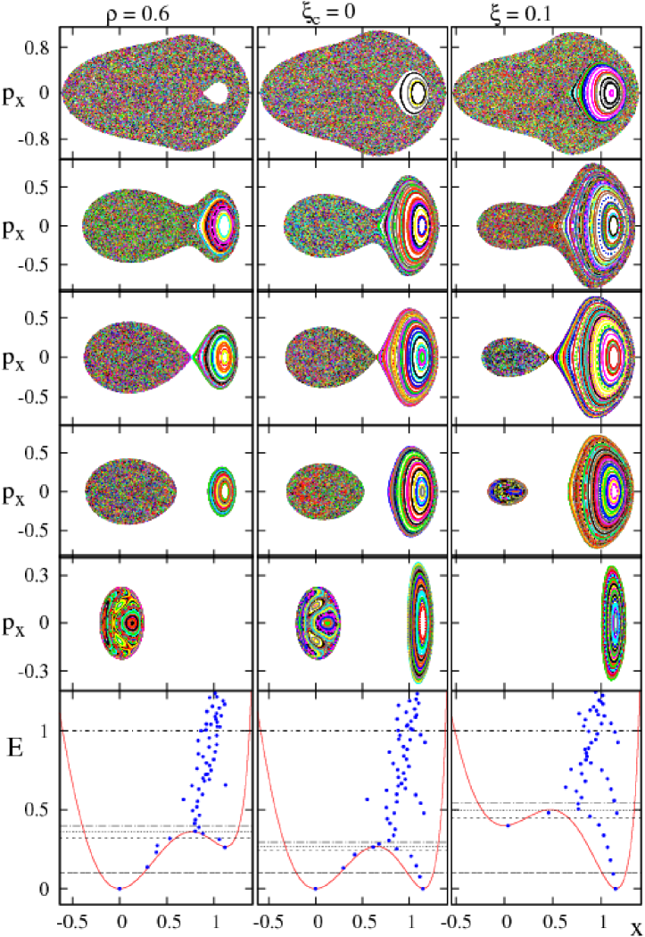
Figure 3: Poincaré sections in the region of phase-coexistence (region II). The panels are as in Fig. 2, but for the classical Hamiltonians ${\cal H}_{1}(\rho)$ (8a) with $\rho^{**}<\rho\leq\rho_{c}$, and ${\cal H}_{2}(\xi)$ (8b) with $\xi_{c}\leq\xi<\xi^{**}$. The classical potentials are $V_{1}(\rho;x,y=0)$ (9a) and $V_{2}(\xi;x,y=0)$ (9b). The Peres lattices involve the quantum Hamiltonians $\hat{H}_{1}(\rho)$ (3a) and $\hat{H}_{2}(\xi)$ (3b).

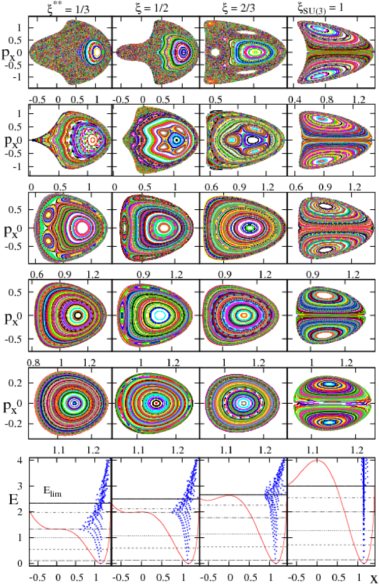
Figure 4: Poincaré sections in the stable deformed phase (region III). The panels are as in Fig. 2, but for the classical Hamiltonian ${\cal H}_{2}(\xi)$ (8b) and potential $V_{2}(\xi;x,y=0)$ (9b), with $\xi\geq\xi^{**}$. The Peres lattices involve the quantum Hamiltonian $\hat{H}_{2}(\xi)$ (3b).

The classical dynamics constraint to $L=0$, can be depicted conveniently via Poincaré surfaces of sections in the plane $y=0$, plotting the values of $x$ and the momentum $p_{x}$ each time a trajectory intersects the plane [25]. Regular trajectories are bound to toroidal manifolds within the phase space and their intersections with the plane of section lie on 1D curves (ovals). In contrast, chaotic trajectories randomly cover kinematically accessible areas of the section.

The Poincaré sections associated with the classical Hamiltonian of Eq. (8) are shown in Figs. 2-3-4 for representative energies, below the domain boundary, and control parameters ($\rho,\xi$) in regions I-II-III, respectively. The bottom row in each figure displays the corresponding classical potential $V(\beta,\gamma\!=\!0)=V(x,y\!=\!0)$, Eq. (9). In region I $(0\leq\rho\leq\rho^{*}$), for $\rho=0$, ${\cal H}_{1}(\rho\!=\!0)={\cal H}_{d,0}(2-{\cal H}_{d,0})$, involves the 2D harmonic oscillator Hamiltonian and $V_{1}(\rho\!=\!0)\!\propto\!2\beta^{2}-\beta^{4}/2$. The system is in the U(5) DS limit and is completely integrable. The orbits are periodic and, as shown in Fig. 2, appear in the surface of section as a finite collection of points. The sections for $\rho\!=\!0.03$ in Fig. 2, show the phase space portrait typical of an anharmonic (quartic) oscillator with two major regular islands, weakly perturbed by the small $\rho\cos 3\gamma$ term. The orbits are quasi-periodic and appear as smooth one-dimensional invariant curves. For small $\beta$, $V_{1}(\rho)\!\approx\!\beta^{2}\!-\!\rho\sqrt{2}\beta^{3}\cos 3\gamma$ and resembles the well-known Hénon-Heiles potential (HH) [26]. Correspondingly, as shown for $\rho\!=\!0.2$ in Fig. 2, at low energy, the dynamics remains regular and two additional islands show up. The four major islands surround stable fixed points and unstable (hyperbolic) fixed points occur in-between. At higher energy, one observes a marked onset of chaos and an ergodic domain. The chaotic component of the dynamics increases with $\rho$ and maximizes at the spinodal point $\rho^{*}\!=\!0.5$. The chaotic orbits densely fill two-dimensional regions of the surface of section.

The dynamics changes profoundly in region II of phase coexistence $(\rho^{*}<\rho\leq\!\rho_{c}$ and $\xi_{c}\leq\xi<\xi^{**})$. The Poincaré sections before at and after the critical point, ($\rho\!=\!0.6$, $\xi_{c}\!=\!0$, $\xi\!=\!0.1$) are shown in Fig. 3. In general, the motion is predominantly regular at low energies and gradually turning chaotic as the energy increases. However, the classical dynamics evolves differently in the vicinity of the two wells. As the local deformed minimum develops, robustly regular dynamics attached to it appears. The trajectories form a single island and remain regular even at energies far exceeding the barrier height $V_{\rm bar}$. This behavior is in marked contrast to the HH-type of dynamics in the vicinity of the spherical minimum, where a change with energy from regularity to chaos is observed, until complete chaoticity is reached near the barrier top. The clear separation between regular and chaotic dynamics, associated with the two minima, persists all the way to the barrier energy, $E=V_{\rm bar}$, where the two regions just touch. At $E>V_{\rm bar}$, the chaotic trajectories from the spherical region can penetrate into the deformed region and a layer of chaos develops, and gradually dominates the surviving regular island for $E\gg V_{\rm bar}$. As $\xi$ increases, the spherical minimum becomes shallower, and the HH-like dynamics diminishes.

Fig. 4 displays the classical dynamics in region III $(\xi^{**}\leq\xi\leq 1)$. The local spherical minimum and the associated HH-like dynamics disappear at the anti-spinodal point $\xi^{**}=1/3$. The regular motion, associated with the single deformed minimum, prevails for $\xi\!\geq\!\xi^{**}$. Here a single stable fixed point, surrounded by a family of elliptic orbits, continues to dominate the Poincaré section. In certain regions of the control parameter $\xi$ and energy, the section landscape changes from a single to several regular islands, reflecting the sensitivity of the dynamics to local degeneracies of normal modes. A notable exception to such variation is the SU(3) DS limit ($\xi=1$), for which the system is integrable and the phase space portrait is the same for any energy.

6 Quantum analysis

Quantum manifestations of classical chaos are often detected by statistical analyses of energy spectra [25]. In a quantum system with mixed regular and irregular states, the statistical properties of the spectrum are usually intermediate between the Poisson and the Gaussian orthogonal ensemble (GOE) statistics. Such global measures of quantum chaos are, however, insufficient to reflect the rich dynamics of an inhomogeneous phase space structure encountered in Figs. 2-4, with mixed but well-separated regular and chaotic domains. To do so, one needs to distinguish between regular and irregular subsets of eigenstates in the same energy intervals. For that purpose, we employ the spectral lattice method of Peres [27], which provides additional properties of individual energy eigenstates. The Peres lattices are constructed by plotting the expectation values $O_{i}=\langle i|\hat{O}|i\rangle$ of an arbitrary operator, $[\hat{O},\hat{H}]\neq 0$, versus the energy $E_{i}=\langle i|\hat{H}|i\rangle$ of the Hamiltonian eigenstates $|i\rangle$. The lattices $\{O_{i},E_{i}\}$ corresponding to regular dynamics can be shown to display an ordered pattern, while chaotic dynamics leads to disordered meshes of points [27, 28].

In the present analysis we choose the Peres operator to be $\hat{n}_{d}$. The lattices correspond to the set of points $\{x_{i},E_{i}\}$, with $x_{i}\equiv\sqrt{2\langle i|\hat{n}_{d}|i\rangle/N}$ and $|i\rangle$ being the eigenstates of the quantum Hamiltonian (3). The expectation value of $\hat{n}_{d}$ in the condensate of Eq. (2) is related to the deformation $\beta$ and the coordinate $x$ in the classical potential (9). Accordingly, the particular choice of lattices $\{x_{i},E_{i}\}$ can distinguish regular from irregular states and associate them with a given region in phase space, through the classical-quantum correspondence $\beta\!=\!x\!\leftrightarrow\!x_{i}$.

The Peres lattices for $L\!=\!0$ eigenstates of the intrinsic Hamiltonian (3) with $N\!=\!80$, are shown on the bottom rows of Figs. 2-4, overlayed on the classical potentials $V(x,y=0)$ of Eq (9). For $\rho\!=\!0$, the Hamiltonian (4) has U(5) dynamical symmetry with a solvable spectrum, a function of $n_{d}$. For large $N$ and replacing $x_{i}$ by $\beta$, the Peres lattice coincides coincides with $V_{1}(\rho=0)$, a trend seen exactly for $\rho=0$ and approximately at $\rho=0.03$ in Fig. 2. For $\rho=0.2$, at low energy a few lattice points still follow the potential curve $V_{1}(\rho)$, but at higher energies one observes sizeable deviations and disordered meshes of lattice points, in accord with the onset of chaos in the classical Hénon-Heiles system. The disorder in the Peres lattice enhances at the spinodal point $\rho^{*}=0.5$, where the chaotic component of the classical dynamics maximizes. As seen in Figs. 3-4, whenever a deformed minimum occurs in the potential, the Peres lattices exhibit regular sequences of states localized within and above the deformed well. They form several chains of lattice points close in energy, with the lowest chain originating at the deformed ground state. A close inspection reveals that the $x_{i}$-values of these regular states, lie in the intervals of $x$-values occupied by the regular tori in the Poincaré sections. Similarly to the classical tori, these regular sequences persist to energies well above the barrier $V_{\rm bar}$. The lowest sequence consists of $L\!=\!0$ bandhead states of the ground $g(K=0)$ and $\beta^{n}(K=0)$ bands. Regular sequences at higher energy correspond to $\beta^{n}\gamma^{2}(K=0)$, $\beta^{n}\gamma^{4}(K=0)$ bands, etc. In contrast, the remaining states, including those residing in the spherical minimum, do not show any obvious patterns and lead to disordered (chaotic) meshes of points at high energy. For $\xi>\xi^{**}$, a larger number and longer sequences of regular $K=0$ bandhead states are observed in the vicinity of the single deformed minimum ($x\approx 1$), as its depth increases.

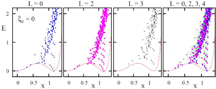
Figure 5: Peres lattices $\{x_{i},E_{i}\}$, for $L=0,2,3,4$, eigenstates of the critical-point Hamiltonian $\hat{H}_{1}(\rho_{c})=\hat{H}_{2}(\xi_{c})$ with $h_{2}=1$ and $N=50$. The right column combines the separate-$L$ lattices and overlays them on the corresponding classical potential.

Peres lattices can also be used to visualize the dynamics of quantum states with non-zero angular momenta. Examples for $N\!=\!50$, $L=0,2,3,4$, eigenstates of the critical-point Hamiltonian, $\hat{H}_{1}(\rho_{c})=\hat{H}_{2}(\xi_{c})$, are shown in Fig. 5. The right column in the figure combines the separate-$L$ lattices and overlays them on the relevant classical potential. Rotational states with $L=0,2,4,\ldots$, comprise the regular $K\!=\!0$ bands mentioned above, and are accompanied by sequences $L=2,3,4,\ldots$, forming $K=2$ bands. Additional $K$-bands (not shown in Fig. 5), corresponding to multiple $\beta$ and $\gamma$ vibrations about the deformed shape, can also be identified. The states in each regular band share a common intrinsic structure, as indicated by their nearly equal values of $\langle\hat{n}_{d}\rangle$ and a similar coherent decomposition of their wave functions in the SU(3) basis, to be discussed in Section 7. These ordered band structures show up in the vicinity of the deformed well and are not present in the disordered (chaotic) portions of the Peres lattice. Their occurrence and persistence in the spectrum throughout the coexistence region, including the critical-point, is somewhat unexpected, in view of the strong mixing and abrupt structural changes taking place.

7 Symmetry aspects

Away from the U(5) and SU(3) limits ($\rho>0$ and $\xi<1$), both dynamical symmetries are broken in the intrinsic Hamiltonian (3). The competition between terms with different symmetry character, drives the system through a first-order QPT with a characteristic pattern of mixed dynamics. It is of great interest to study the symmetry properties of the Hamiltonian eigenstates across the QPT and, in particular, seek for a symmetry-based explanation for the persistence of regular subsets of states amidst a complicated environment.

Consider an eigenfunction of the Hamiltonian, $|L_{i}\rangle$, with angular momentum $L$ and ordinal number $i$ (enumerating the occurrences of states with the same $L$, with increasing energy). Its expansion in the U(5) DS basis, $|N,n_{d},\tau,n_{\Delta},L\rangle$ of Eq. (1a), and in the SU(3) DS basis, $|N,(\lambda,\mu),K,L\rangle$ of Eq. (1b), reads

$$|L_{i}\rangle = \sum_{n_{d},\tau,n_{\Delta}}C^{(L_{i})}_{n_{d},\tau,n_{\Delta}}|N,n_{d},\tau,n_{\Delta},L_{i}\,\rangle~{},$$ (11)

$$= \sum_{(\lambda,\mu),K}C^{(L_{i})}_{(\lambda,\mu),K}|N,(\lambda,\mu),K,L_{i}\,\rangle~{}.$$

The U(5) ($n_{d}$) probability distribution, $P_{n_{d}}^{(L_{i})}$, and the SU(3) [$(\lambda,\mu)$] probability distribution, $P_{(\lambda,\mu)}^{(L_{i})}$, are calculated as

$$P_{n_{d}}^{(L_{i})} = \sum_{\tau,n_{\Delta}}|C^{(L_{i})}_{n_{d},\tau,n_{\Delta}}|^{2}~{},$$ (12a)

$$P_{(\lambda,\mu)}^{(L_{i})} = \sum_{K}|C^{(L_{i})}_{(\lambda,\mu),K}|^{2}~{}.$$ (12b)

The purity of eigenstates with respect to a DS basis can be evaluated by means of the U(5) and SU(3) Shannon entropies defined as

$$S_{\mathrm{U5}}(L_{i}) = -\frac{1}{\ln D_{5}}\sum_{n_{d}}P_{n_{d}}^{(L_{i})}\ln P_{n_{d}}^{(L_{i})}~{},$$ (13a)

$$S_{\mathrm{SU3}}(L_{i}) = -\frac{1}{\ln D_{3}}\sum_{(\lambda,\mu)}P_{(\lambda,\mu)}^{(L_{i})}\ln P_{(\lambda,\mu)}^{(L_{i})}~{}.$$ (13b)

The normalization $D_{5}$ ($D_{3}$) counts the number of possible $n_{d}$ [$(\lambda,\mu)$] values for a given $L$. A Shannon entropy vanishes when the considered state is pure with good $G$-symmetry [$S_{\mathrm{G}}(L_{i})\!=\!0$], and is positive for a mixed state. The maximal value [$S_{\mathrm{G}}(L_{i})\!=\!1$] is obtained when $|L_{i}\rangle$ is uniformly spread among the irreps of $G$, i.e. for $P_{G}^{(L_{i})}\!=\!1/D_{G}$. Intermediate values, $0<S_{\mathrm{G}}(L_{i})<1$, indicate partial fragmentation of the state $|L_{i}\rangle$ in the respective DS basis.

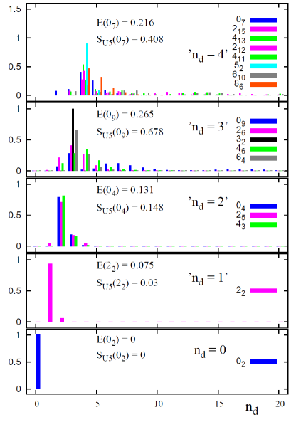
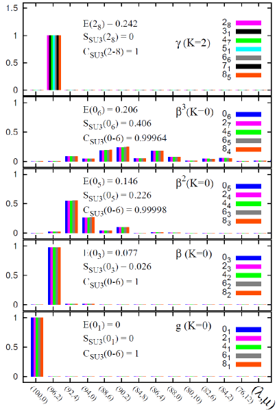
Figure 6: U(5) $n_{d}$-probability distribution, $P_{n_{d}}^{(L_{i})}$ (12a) [left column], and SU(3) $(\lambda,\mu)$-probability distribution, $P_{(\lambda,\mu)}^{(L_{i})}$ (12b) [right column], for selected eigenstates of the critical-point $(\rho_{c},\xi_{c})$ Hamiltonian (3), with $N=50$. The U(5) Shannon entropy, $S_{\rm U5}(L_{i})$ (13a), and SU(3) correlator, $C_{\rm SU3}(0{\rm-}6)$ (14), are indicated for spherical and deformed type of states, respectively.

Focusing on the critical-point Hamiltonian, the states shown on the left column of Fig. 6 were selected on the basis of having the largest components with $n_{d}=0,1,2,3,4$, within the given $L$ spectra. States with different $L$ values are arranged into panels labeled by ‘$n_{d}$’ to conform with the structure of the $n_{d}$-multiplets of the U(5) DS limit, Eq. (4). Each panel depicts the U(5) $n_{d}$-probabilities, $P_{n_{d}}^{(L_{i})}$ (12a), for states in the multiplet and lists the U(5) Shannon entropy $S_{\rm U5}(L_{i})$ of a representative eigenstate. In particular, the zero-energy $L\!=\!0^{+}_{2}$ state is seen to be a pure $n_{d}\!=\!0$ state, with $S_{\rm U5}\!=\!0$, which is the solvable U(5)-PDS eigenstate of Eq. (5a). The state $2^{+}_{2}$ has a pronounced $n_{d}\!=\!1$ component (96%) and the states ($L=0^{+}_{4},\,2^{+}_{5},\,4^{+}_{3}$) in the third panel, have a pronounced $n_{d}\!=\!2$ component and a low value of $S_{\rm U5}<0.15$. All the above states with $`n_{d}\leq 2^{\prime}$ have a dominant single $n_{d}$ component, and hence qualify as ‘spherical’ type of states. These multiplets comprise the lowest left-most states shown in the combined Peres lattices of Fig. 5. In contrast, the states in the panels ‘$n_{d}=3$’ and ‘$n_{d}=4$’ of Fig. 6, are significantly fragmented. Notable exceptions are the $L=3^{+}_{2}$ state, which is the solvable U(5)-PDS state of Eq. (5b) with $n_{d}=3$, and the $L=5^{+}_{2}$ state with a dominant $n_{d}=4$ component. The existence in the spectrum of specific spherical-type of states with either $P_{n_{d}}^{(L)}\!=\!1$ $[S_{\rm U5}(L)\!=\!0]$ or $P_{n_{d}}^{(L)}\approx 1$ $[S_{\rm U5}(L)\approx 0]$, exemplifies the presence of an exact or approximate U(5) PDS at the critical-point.

The states shown on the right column of Fig. 6 have a different character. They belong to the five lowest regular sequences seen in the combined Peres lattices of Fig. 5. They have a broad $n_{d}$-distribution, hence are qualified as ‘deformed’-type of states, forming rotational bands: $g(K\!=\!0),\,\beta(K\!=\!0),\,\beta^{2}(K\!=\!0),\,\beta^{3}(K\!=\!0)$ and $\gamma(K\!=\!2)$. Each panel depicts the SU(3) $(\lambda,\mu)$-distribution, $P_{(\lambda,\mu)}^{(L_{i})}$ (12b) for the rotational states in each band. The ground $g(K=0)$ and the $\gamma(K=2)$ bands are pure $[S_{\rm SU3}=0$] with $(\lambda,\mu)=(2N,0)$ and $(2N-4,2)$ SU3) character, respectively. These are the solvable bands of Eq. (7) with SU(3) PDS. The non-solvable $K$-bands are mixed with respect to SU(3), but the mixing is similar for the different $L$-states in the same band. Such strong but coherent ($L$-independent) mixing is the hallmark of SU(3) quasi-dynamical symmetry (QDS). It results from the existence of a single intrinsic state for each such band and imprints an adiabatic motion and increased regularity [29].

The coherent decomposition characterizing SU(3) QDS, implies strong correlations between the SU(3) components of different $L$-states in the same band. This can be used as a criteria for the identification of rotational bands. We focus here on the $L=0,2,4,6$, members of $K=0$ bands. Given a $L=0^{+}_{i}$ state, among the ensemble of possible states, we associate with it those $L_{j}>0$ states which show the maximum correlation, $\max_{j}\{\pi(0_{i},L_{j})\}$. Here $\pi(0_{i},L_{j})$ is a Pearson coefficient whose values lie in the range $[-1,1]$. Specifically, $\pi(0_{i},L_{j})=1,-1,0,$ indicate a perfect correlation, a perfect anti-correlation, and no linear correlation, respectively, among the SU(3) components of the $0_{i}$ and $L_{j}$ states. To quantify the amount of coherence (hence of SU(3)-QDS) in the chosen set of states, we employ the following product of the maximum correlation coefficients [30]

$$C_{\rm SU3}(0_{i}{\rm-}6)\equiv\max_{j}\{\pi(0_{i},2_{j})\}\,\max_{k}\{\pi(0_{i},4_{k})\}\,\max_{\ell}\{\pi(0_{i},6_{\ell})\}~{}.$$ (14)

We consider the set of states $\{0_{i},\,2_{j},\,4_{k},\,6_{\ell}\}$ as comprising a $K=0$ band with SU(3)-QDS, if $C_{\rm SU3}(0_{i}{\rm-}6)\approx 1$. As expected, we find the values $C_{\rm SU3}(0_{i}{\rm-}6)\approx 1$ for all the ‘deformed’ $K$-bands, shown in the right column of Fig. 6. It should be noted that the coherence property of a band of states, as measured by $C_{\rm SU3}(0_{i}{\rm-}6)$, is independent of its purity, as measured by $S_{\rm SU3}(L_{i})$. Thus, in Fig. 6, the pure $g(K=0)$ and $\gamma(K=2)$ bands with SU(3) PDS have $C_{\rm SU3}(0_{i}{\rm-}6)=1$ and $S_{\rm SU3}=0$, while the mixed $\beta^{3}(K=0)$ band has $C_{\rm SU3}(0_{i}{\rm-}6)=0.9996$ and $S_{\rm SU3}=0.406$.

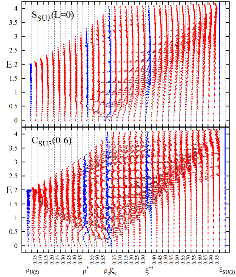
Figure 7: SU(3) Shannon entropy $S_{\rm SU3}(L\!=\!0)$ (13b) [top panel], and SU(3) correlator, $C_{\rm SU3}(0{\rm-}6)$ (14) [bottom panel] for energy eigenstates of the Hamiltonian (3) with $N\!=\!50$, as a function of the control parameters $(\rho,\xi)$. The vertical dashed lines are explained in the text.

The top panel of Fig. 7 displays the values of the SU(3) Shannon entropy (13b) for $L=0$ eigenstates of the Hamiltonian (3), with $N=50$. The vertical axis lists the energy $E$ of the states, while the horizontal axis lists 35 values of the control parameters $(\rho,\xi)$. Vertical dashed lines which embrace each control parameter, correspond to the value $S_{SU3}(L\!=\!0)=0$ (left) and $S_{SU3}(L\!=\!0)=1$ (right). Thus, states which are pure with respect to SU(3) are represented by points on the vertical dashed line to the left of the given control parameter. Departures from this vertical line, $0<S_{SU3}(L\!=\!0)\leq 1$, indicate the amount of SU(3) mixing. The bottom panel of Fig. 7, displays the values of the SU(3) correlation coefficient $C_{\mathrm{SU3}}(0{\rm-}6)$, Eq. (14), correlating sequences of $L=0,2,4,6$ states, throughout the entire spectrum. The energy $E$, listed on the vertical axis, corresponds to the energy of the $L=0$ eigenstate in each sequence. The vertical dashed lines correspond now to the value $C_{\mathrm{SU3}}(0{\rm-}6)=1$ (right) and $C_{\mathrm{SU3}}(0{\rm-}6)=0$ (left). Thus, a highly-correlated sequence of $L=0,2,4,6$ states, comprising a $K=0$ band and manifesting SU(3)-QDS, are represented by points lying on or very close to the vertical dashed line to the right of the given control parameter, corresponding to $C_{\rm SU3}(0{\rm-}6)\approx 1$. Slight departures from this vertical line, $C_{\rm SU3}(0{\rm-}6)<1$, indicate a reduction of SU(3) coherence.

At the SU(3) DS limit ($\xi_{\rm SU(3)}=1$), the SU(3) entropy, $S_{\rm SU3}(L)=0$, vanishes for all states. In this case, the $L$-states in a given $K$-band belong to a single SU(3) irrep, hence necessarily $C_{\rm SU3}(0{\rm-}6)=1$. For $\xi<1$, $S_{\rm SU3}(L\!=0)>0$ acquires positive values, reflecting an SU(3) mixing. The SU(3) breaking becomes stronger at higher energies and as $\xi$ approaches $\xi_{c}=0$ from above, resulting in higher values of $S_{\rm SU3}(L\!=\!0)$. A notable exception to this behavior is the deformed ground state ($L=0_{1}$) of $\hat{H}_{2}(\xi)$, which maintains $S_{\rm SU3}(L\!=\!0_{1})=0$ throughout region III ($\xi^{**}\leq\xi\leq 1$) and in part of region II ($\xi_{c}\leq\xi<\xi^{**}$), in accord with its SU(3)-PDS property, Eq. (7a). In contrast to the lack of SU(3)-purity in all excited $L=0$ states, the SU(3) correlation function maintains a value close to unity, $C_{\mathrm{SU3}}(0{\rm-}6)\approx 1$. This indicates that the SU(3) mixing is coherent and that these $L=0$ states serve as bandhead states of $K=0$ bands with a pronounced SU(3) QDS. This band-structure is observed throughout region III in extended energy domains, consistent with the classical analysis, which revealed a robustly regular dynamics in this region.

In region I ($0\leq\rho\leq\rho^{*}$), all states show high values of $S_{\rm SU3}(L\!=\!0)\approx 1$ and $C_{\rm SU3}(0{\rm-}6)<1$, indicating considerable SU(3) mixing and lack of SU(3) coherence. This is in line with the presence of spherical-states, at low energy, and of more complex-type of states at higher energy, and the absence of rotational bands in this region. In region II of phase coexistence ($\rho^{*}<\rho\leq\rho_{c}$ and $\xi_{c}\leq\xi<\xi^{**}$), one encounters both points with $C_{\rm SU3}(0{\rm-}6)\approx 1$, and points with $C_{\rm SU3}(0{\rm-}6)<1$. This reflects the presence of deformed states arranged into regular bands, exemplifying SU(3) QDS, and at the same time, the presence of spherical states and other states of a different nature. These results highlight the relevance of U(5)-PDS (partial purity) and SU(3)-QDS (coherence) for clarifying the survival of regular subsets of states in the presence of more complicated type of states, a situation encountered in QPTs of non-integrable systems.

This work is supported by the Israel Science Foundation. M.M. acknowledges the Golda Meir Fellowship Fund and the Czech Science Foundation (P203-13-07117S).

References

- [1] Hertz J A 1976 Phys. Rev. B 14 (1976) 1165
- [2] Gilmore R and Feng D H 1978 Nucl. Phys. A 301 189; Gilmore R 1979 J. Math. Phys. 20 891
- [3] Carr L ed 2010 Understanding Quantum Phase Transitions (CRC press)
- [4] S. Sachdev 1999 Quantum Phase Transitions (Cambridge: Cambridge Univ. Press)
- [5] Marianetti C A , Kotliar G and Ceder G 2004 Nature Mater. 3 627
- [6] Pfleiderer C 2009 Rev. Mod. Phys. 81 1551
- [7] Karmakar B, Pellegrini V, Pinczuk A, Pfeiffer L N and West K W 2009 Phys. Rev. Lett. 102 036802
- [8] Cejnar P, Jolie J and Casten R F 2010 Rev. Mod. Phys. 82 2155
- [9] Emary C and Brandes T 2003 Phys. Rev. Lett. 90 044101; Phys. Rev. E 67 066203
- [10] Macek M and Leviatan A 2011 Phys. Rev. C 84 041302(R)
- [11] Leviatan A and Macek M 2012 Phys. Lett. B 714 110
- [12] Macek M and Leviatan A 2013 in preparation
- [13] Iachello F and Arima A 1987 The Interacting Boson Model (Cambridge: Cambridge Univ. Press)
- [14] Bohr A and Mottelson B R 1998 Nuclear Structure Vol. II (Singapore: World Scientific)
- [15] Ginocchio J N and Kirson M W 1980 Phys. Rev. Lett. 44 1744
- [16] Dieperink A E L, Scholten O and Iachello F 1980 Phys. Rev. Lett. 44 1747
- [17] Cejnar P and Jolie J 2009 Prog. Part. Nucl. Phys. 62 210
- [18] Leviatan A 1996 Phys. Rev. Lett. 77 818; Leviatan A 2011 Prog. Part. Nucl. Phys. 66 93
- [19] Rowe D J 2004 Phys. Rev. Lett. 93 122502; Rosensteel G and Rowe D J 2005 Nucl. Phys. A 759 92
- [20] Leviatan A 2007 Phys. Rev. Lett. 98 242502
- [21] Leviatan A Ann. Phys. (NY) 179 201
- [22] Leviatan A 2006 Phys. Rev. C 74 051301(R)
- [23] Hatch R L and Levit S 1982 Phys. Rev. C 25 614
- [24] Whelan N and Alhassid Y 1993 Nucl. Phys. A 556 42
-
[25]
Reichl L E 1992
The Transition to Chaos in Conservative Classical Systems:
Quantum Manifestations,
(New York: Springer-Verlag). - [26] Hénon M H and Heiles C 1964 Astron. J. 69 73
- [27] A. Peres A 1984 Phys. Rev. Lett. 53 1711
- [28] Stránský P, Hruška P and Cejnar P 2009 Phys. Rev. E 79 066201
- [29] Macek M, Dobeš J , Stránský P and Cejnar P 2010 Phys. Rev. Lett. 105 072503
- [30] Macek M, Dobeš J and Cejnar P 2010 Phys. Rev. C 82 014308