Exit probability in inflow dynamics: nonuniversality induced by range, asymmetry and fluctuation

Abstract

Probing deeper into the existing issues regarding the exit probability (EP) in one dimensional dynamical models, we consider several models where the states are represented by Ising spins and the information flows inwards. At zero temperature, these systems evolve to either of two absorbing states. The exit probability $E(x)$, which is the probability that the system ends up with all spins up starting with $x$ fraction of up spins is found to have the general form $E(x)=x^{\alpha}/\left[x^{\alpha}+(1-x)^{\alpha}\right]$. The exit probability exponent $\alpha$ strongly depends on $r$, the range of interaction, the symmetry of the model and the induced fluctuation. Even in a nearest neighbour model, nonlinear form of EP can be obtained by controlling the fluctuations and for the same range, different models give different results for $\alpha$. Non-universal behaviour of the exit probability is thus clearly established and the results are compared to existing studies in models with outflow dynamics to distinguish the two dynamical scenarios.

There are many systems in condensed matter physics, magnetism, biology and social phenomena bio ; gen-dyn ; book ; soc2 which are found to reach an ordered state following certain dynamical rules. The dynamical rules represent the mechanisms by which macroscopic structures are generated from the microscopic interactions. The role of the dynamics is reflected in the scaling behaviour of relevant variables. Often we note power law scaling behaviour, e.g. in coarsening phenomena, domains grow in a power law manner with time. If two different dynamical schemes lead to identical behaviour of the relevant variables one may conclude that the two schemes are actually equivalent. However, careful studies are required to establish such equivalence.

Of late, a debate on whether inflow dynamics is different from outflow dynamics has emerged glauber ; sznajd ; krupa ; cas . Precisely, in models involving spins, when the state of the central spin is dictated by its neighbours, it is a case of inflow of information. Outflow of information occurs when a group of neighbouring spins dictates the state of all other spins neighbouring them. To settle the debate, the exit probability (EP) is one of the features which is studied when the spins can be in up or down states. Starting with $x$ fraction of spins in the up state, exit probability $E(x)$ is the probability to reach a final state with all spins up.

The Ising-Glauber model glauber is an example of inflow dynamics where the local field determines whether a spin will flip or not. An example where outflow of information takes place is the Sznajd model sznajd . In the Ising-Glauber model, a spin is selected randomly and its state is updated following an energy minimisation scheme. In one dimension, this always leads to either of two absorbing states: all spins up or all down. In the Sznajd model, a plaquette of neighbouring spins is considered, if they agree then the spins on the boundary of the plaquette are oriented along them. In one-dimension, the plaquette is a panel of two spins. The Sznajd model has the same two absorbing states as in the Ising model. The two models also have identical exponents associated with domain growth and persistence behaviour during coarsening behera ; stauffer1 . However, a few other dynamic quantities were shown to be different for generalised models with inflow and outflow dynamics where a suitable parameter associated with the spin flip probability was introduced godreche ; krupa . The Ising Glauber and Sznajd models can be obtained by choosing specific values of the parameters in the generalised models with inflow and outflow dynamics respectively.

The exit probability plays an important role in the debate as it shows a marked difference in behaviour for the two models: for the Ising Glauber model, EP is linear; $E(x)=x$ while for the Sznajd model slanina ; redner ; cas

$$E(x)=\frac{x^{2}}{x^{2}+(1-x)^{2}},$$ (1)

a distinctly nonlinear function of $x$.

Another version of a generalised model with inflow and outflow dynamics was proposed more recently cas in which the range $r$ of the interaction was varied. The Sznajd model with range $r$ (S(r) model hereafter) showed a range independent behaviour of the exit probability; EP is given by eq. (1) for all $r$. For the generalised Ising Glauber model with $r$ neighbours (G(r) model henceforth), numerical simulations were made which showed very good fitting to the form given in eq. (1) for $r=2$ from which it was claimed that non-linear behaviour of $E(x)$ can be observed for inflow dynamics as well.

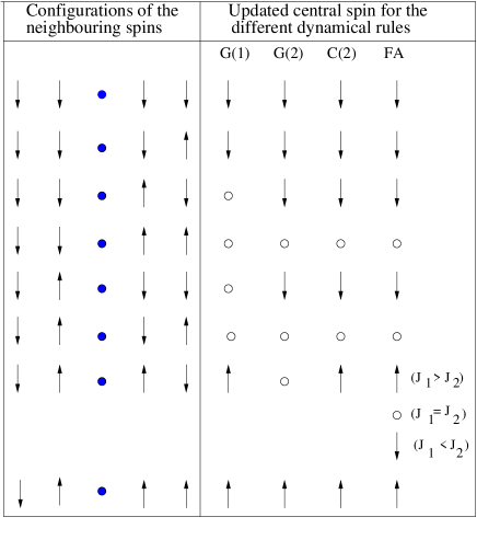
Figure 1: (Color online) Left panel shows configuration of the neighbouring spins of the central spin represented by a •which means either of the up/down states at time $t$. Right panel shows the state of the central spin after it is updated according to the different dynamical rules. A $\circ$ implies an “undecided” state when the up/down state occurs with equal probability. The other eight states can be obtained by inversion.

A generalised $q$-voter model which involves outflow dynamics has also been proposed qvoter in which $q$ neighbouring spins, if they agree, influence their other neighbouring spins. In one dimension, $q=2$ corresponds to the Sznajd model and the random version with $q=1$ (where only one of the two boundary spins is updated with equal probability) corresponds to the Ising Glauber/voter model. The exit probability here again showed the property that it is independent of range.

The shape of the exit probability is an important issue. Another interesting point to be noted is, in all the different models studied so far cas ; redner ; slanina ; qvoter in one dimension, no finite size dependence has been noted in EP. However, there is a school of thought that such effects do exist and in reality exit probability has a step function behaviour in the thermodynamic limit galam as observed in higher dimensions stauffer ; networks ; cas2d . Such a step function behaviour also occurs for a special class of one-dimensional models where the dynamical rule involves the size of the neighbouring domains bss ; rbs . However, in the present work, we consider only those models with inflow dynamics (all of which are short ranged) which belong to the Ising-Glauber class as far as dynamical behaviour is concerned. Our aim is to find out how EP depends on various factors incorporated in the dynamics. Our main result is that a general form for the exit probability given by

$$E(x)=\frac{x^{\alpha}}{x^{\alpha}+(1-x)^{\alpha}}$$ (2)

exists, where $\alpha$, the so called exit probability exponent is very much dependent on factors like the range of interaction, asymmetry of the model and fluctuation present in the dynamics.

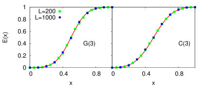
Figure 2: (Color online) Exit probability versus initial concentration of up spins in the generalised Ising (G(r); left panel) and cutoff models (C(r); right panel) with $r=3$. The $L=1000$ curves are fitted with the best fit line of the form given in eq. (2).

Models and results:
1. The Ising Glauber model with $r$ neighbours (G(r)) : To update the $i$th spin $s_{i}(=\pm 1)$ here, one computes

$$x=\sum_{j=1}^{r}[s_{i+j}+s_{i-j}].$$ (3)

If $x>0,s_{i}=1$, if $x<0,s_{i}=-1$ and $s_{i}$ is flipped with probability 1/2 if $x=0$. For G(r), results are known for $r=1$ (exact) book and $2$ (numerical) cas . We have obtained results for higher values of $r$.
2. The cutoff model: A model with a cutoff at $r$ called the C(r) model proposed in biswas-sen2 was also studied. Here only the spins sitting at the domain boundary are liable to flip. To update such a spin on site $i$, we calculate two quantities $r_{1}$ and $r_{2}$. $r_{1}$ is determined from the condition
$s_{i+1}=s_{i+2}=\cdots=s_{i+r_{1}}\neq s_{i+r_{1}+1}$;
and similarly $r_{2}$ is calculated from the spins on the left side of the $i$th spin. $r_{1}$ and $r_{2}$ are both restricted to a maximum value $r$. Hence the neighbouring domain sizes $r_{1}$ and $r_{2}$ are calculated subject to the restriction that the maximum size is $r$. When $r_{1}$ is greater (less) than $r_{2}$, the state of the right (left) neighbours is adopted. If $r_{1}=r_{2}$, the spin is flipped with probability 1/2. C(r) is equivalent to G(r) for $r=1$.
3. The ferromagnetic asymmetric next nearest model (FA) model: The G(2) or C(2) models can in fact be shown to be special cases of the Ising model with second neighbour interaction. The Hamiltonian for this model is

$$H=-J_{1}\sum_{i}s_{i}s_{i+1}-J_{2}\sum_{i}s_{i}s_{i+2}.$$ (4)

Here, the role of asymmetry can be studied by varying $\kappa=J_{2}/J_{1}$. The special case $\kappa=1$ is identical to G(2). $\kappa<1$ corresponds to C(2) and for $\kappa>1$ one may expect a different behaviour. This system can be regarded as a ANNNI chain selke with both interactions positive (ferromagnetic). By definition the FA model has range $r=2$.
4. The W(r) model: The W(r) model is exactly like the Ising Glauber model except for the fact that when $x=0$ in eq. (3), the spins are flipped with probability $W_{0}$ godreche . It is known that for $W_{0}=0$, which is called the constrained Glauber model, absorbing states are frozen states which are not the all up/down states. $W_{0}=0.5$ corresponds to the Ising Glauber model while $W_{0}=1$ is the case of Metropolis rule. $W_{0}$ in a sense quantifies the fluctuation induced by the dynamics, the fluctuation is maximum when $W_{0}=1$ which causes the spins to flip whenever $x$ in eq. (3) equals zero. In this model, we have studied the case for $r\geq 1$.

In Fig. 1, we have presented the possible updated configurations for the central spin corresponding to eight different configurations of its 4 nearest neighbours for G(1), G(2), C(2) and FA. The other eight cases can be obtained by inverting all the spins. It is immediately noted that G(r) and C(r) differ even for $r=2$. For FA, we may expect a new value of $\alpha$ for $\kappa>1$, which, however, should not depend on the exact value of the $\kappa$. It is also seen that the central spin is “undecided” in maximum number of cases in G(1), such cases are less in number for G(2) and even less in C(2) and FA with $\kappa\neq 1$. We will discuss the effect of this feature on EP later.

As mentioned before, the EP follows a behaviour given by eq. (2) in all cases. Typical variation of the EP for G(r) and C(r) for $r=3$ are shown in Fig. 2. In Fig. 3, we plot the values of $\alpha$ against $r$ for these two models. We note that $\alpha$ is an increasing function of $r$ for both models. Hence $\alpha$ for G(r) is greater than 2 for $r>2$ and the value of $\alpha=2$ coincides with the S(r) value only for $r=2$. On the other hand, $\alpha$ for C(r) is less compared to G(r) for all $r>1$. We try a general form to fit $\alpha$ with $r$ as

$$(\alpha-1)=a(r-1)^{b}$$ (5)

and note that it shows a fairly good fitting for both G(r) and C(r) with $a=1.04\pm 0.02$, $b=0.66\pm 0.02$ for G(r) and $a=0.85\pm 0.01$, $b=0.56\pm 0.01$ for C(r). Both $a$ and $b$ are larger for G(r) indicating the stronger dependence on $r$.

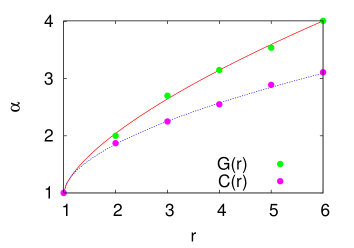
Figure 3: (Color online) Plot of the exponent $\alpha$ against range $r$ for $G(r)$ and $C(r)$ models. The full line corresponds to the fitting form of eq.(5)

.

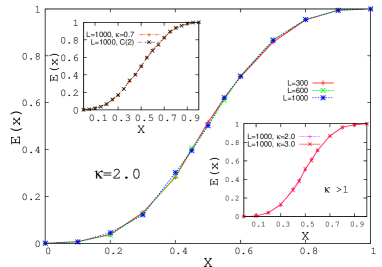
Figure 4: (Color online) Exit probability for the FA model: main plot shows the result for $\kappa=2$ for different system sizes. Top left inset shows $E(x)$ for $\kappa<1$ and C(2) which give identical results as expected; bottom right inset shows that for $\kappa>1$, EP is independent of the exact value of $\kappa$. The solid lines are guides to the eye.

The FA model, as expected, gives $\alpha=1.85\pm 0.03$ for $\kappa<1$ which is identical to the C(2) value ($1.85\pm 0.02$) and $\alpha=2$ for $\kappa=1$ (the G(2) model). In the third case $\kappa>1$, we get a new value of $\alpha=2.24\pm 0.04$. The results are shown in Fig. 4.

The W(r) model leads to both qualitatively and quantitatively different results. Even for $r=1$, the exit probability does not have a linear dependence on $x$ for $W_{0}\neq 0.5$; $\alpha\neq 1$ unlike the Ising-Glauber case (Fig. 5). Here too we find $\alpha$ to be dependent on $r$. We plot the dependence of $\alpha$ against $W_{0}$ for $r=1,2$ and $3$ in Fig. 6. For the W(1) model, $\alpha$ behaves as $1/\sqrt{2W_{0}}$ as $W_{0}\to 1$. The values of $\alpha$ for $r=2$ and $r=1$ differ by unity for any $W_{0}$ as in the Ising Glauber model. However, the differences in the values of $\alpha$ for W(3) and W(2) weakly increase with $W_{0}$. It is interesting to note here that Glauber ($W_{0}=0.5$) and Metropolis ($W_{0}=1$) algorithms give different values of $\alpha$ although for any $W_{0}\neq 0$, the W(r) model belongs to the Glauber universality class godreche .

Some general features can immediately be noted from the results. If $r$ is increased, $\alpha$ increases indicating that the exit probability becomes steeper in models with inflow dynamics. When $r$ is same in two models, $\alpha$ assumes different values due to the presence of other factors. For example, both $G(2)$ and FA ($\kappa>1$) have $r=2$, but $\alpha$ is larger in the latter. The two models differ in the number of so called “undecided states” (see Fig. 1) and apparently $\alpha$ is larger when such states are less in number. In order to account for the fact that C(2) has a smaller value of $\alpha$ compared to G(2), although the number of undecided states is less here, one must also note that the effective number of neighbours in C(2) is less than 2. The combined effect makes the value of $\alpha$ smaller indicating that the range has a stronger effect on EP than stochasticity.

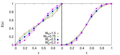
Figure 5: (Color online) Exit probability versus initial concentration of up spins in the W(r) model, $r=1$ (left panel) and $r=2$ (right panel). The solid lines are guides to the eye.

The results in the W(r) model can be qualitatively explained. For $r=1$, we note that the EP curves have different curvature for $W_{0}$ below and above $W_{0}=0.5$. Let us take the case when $x<0.5$ where EP is larger for $W_{0}>0.5$ compared to the value at $W_{0}=0.5$. This happens since the initial state here contains more spins in the down state, and the flipping probability is larger than 1/2. Same logic explains why EP is less when $x>0.5$. At $x=0.5$, $E(x)$ is equal to 1/2 for all models as $E(x)+E(1-x)=1$. So the curves cross at $x=0.5$ and $\alpha$ has a smaller value than 1 for $W_{0}>0.5$ and larger value than 1 for $W_{0}<0.5$ (as for $W_{0}=0.5,~{}E(x)=x$, or $\alpha=1$). $W_{0}$ effectively controls the fluctuation and we find that it can alter the value of $\alpha$. For larger values of $r$, similarly, $\alpha$ is larger (smaller) than the G(r) values for $W_{0}<0.5$ ($W_{0}>0.5$). However, the curvatures are same as $\alpha>1$ always.

We also note that no system size dependence of the EP is observed in any of the models even when $r$ is increased, asymmetry is introduced or fluctuation is modified. So no indication of a step function like EP is there for finite values of $r$ even in the thermodynamic limit. However, as $r$ is made larger, $\alpha$ increases and one can conclude that in the fully connected model corresponding to the infinite dimensional case, $\alpha$ will diverge giving rise to a step function behaviour in the EP at $x=1/2$.

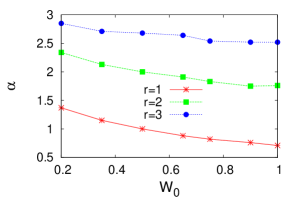
Figure 6: (Color online) Exponent $\alpha$ against $W_{0}$ in the W(r) model with $r=1$, $2$ and $3$. The solid lines are guides to the eye.

Some of the issues discussed in the beginning may be addressed now. First of all, it is evident that EP shows range dependence in models with inflow of information in general in contrast to models with outflow of information, where increasing the range only results in change in timescales. In inflow dynamics, increasing $r$ apparently makes the system approach higher dimensional behaviour, although no system size dependence appears. The fact that EP for S(r) and G(2) model cas ; qvoter ; slanina shows identical behaviour ($\alpha=2$) seems to be purely accidental; there are inflow and outflow models with $r=2$ which have $\alpha\neq 2$. However, $\alpha$ can be nonintegral in inflow dynamics in contrast to known models with outflow dynamics cas ; qvoter ($\alpha=q$ for the $q$ voter model).

An important issue is the question of universality. As already mentioned, all the models studied here have the same dynamical behaviour as far as coarsening is concerned; they all belong to the Ising-Glauber class with the dynamic exponent and persistence exponent identical. In fact, even the models with outflow dynamics like the Sznajd model belongs to this universality class stauffer1 (we have checked for $r=2$ as well). Thus we find that the exit probability is a nonuniversal quantity, it depends on the details of the dynamical rule and is not simply determined by the fact whether information flows out or in. However, it seems safe to make the statement that there is a clear difference: outflow dynamics is characterised by no range dependence while inflow dynamics is.

The question that may naturally arise after this discussion is why does the EP behave differently when the coarsening behaviour is identical. Here it should be remembered that coarsening behaviour is strictly relevant to a completely random initial configuration corresponding to $x=1/2$. Indeed, at $x=1/2$, in all the cases $E(x)=1/2$. Hence a deviation from the perfectly random state results in reaching the all up/down states with different probabilities for the different models.

In summary, we present evidence that the exit probability can be expressed in a general form. An exponent $\alpha$ associated with the EP is identified which is strongly dependent on the details of the system as far as inflow dynamics is concerned. $\alpha$ can have nonintegral values (even less than unity) for inflow dynamics while for the models with outflow dynamics studied so far, only integral values have been obtained. Most of the observed results can be qualitatively explained.

The range dependence distinguishes the inflow dynamics from outflow dynamics. Apart from the range dependence, the role of other factors in the dynamical rules also show their effect on EP in inflow dynamics. Effect of these factors in outflow dynamics may bring out further distinguishing features, a study in progress rb .

Acknowledgement: PR acknowledges financial support from UGC. PS acknowledges financial support from CSIR project. S.B. thanks the Department of Theoretical Physics, TIFR, for the use of its computational resources.

References

- (1) A. M. Turing, Phil. Trans. Roy. Soc. B 237, 37 (1952).
- (2) A. J. Bray, Adv. Phys. 43, 357 (1994).
- (3) P. Sen and B. K. Chakrabarti, Sociophysics: An Introduction (2013).
- (4) C. Castellano, S. Fortunato, and V. Loreto, Rev. Mod. Phys. 81, 591 (2009).
- (5) R. J. Glauber, J. Math. Phys. 4, 294 (1963).
- (6) K. Sznajd-Weron and J. Sznajd, Int. J. Mod. Phys. C 11, 1157 (2000).
- (7) K. Sznajd-Weron and S. Krupa, Phys. Rev. E 74, 031109 (2006).
- (8) C. Castellano and R. Pastor-Satorras, Phys. Rev. E 83, 016113 (2011).
- (9) Behera, L., Schweitzer, F. On spatial consensus formation: Is the Sznajd model different from a voter model? Int. J. Mod. Phys. C 14, 1331 (2003).
- (10) D. Stauffer and P.M.C. de Oliveira, Eur. Phys. J. B 30, 587–592 (2002).
- (11) C. Godréche and J. M. Luck, J. Phys: Condens. Matter 17, S2573 (2005).
- (12) R. Lambiotte and S. Redner, Europhys. Lett. 82, 18007 (2008).
- (13) F. Slanina, K. Sznajd-Weron and P. Przybyla, Europhys. Lett. 82, 18007 (2008).
- (14) P. Przybyla, K. Sznajd-Weron, M. Tabiszewski, Phys. Rev. E 84, 031117 (2011).
- (15) S. Galam and A. C. R.Martins, Europhys. Lett. 95, 48005 (2011) and the references therein.
- (16) D. Stauffer, A. O. Sousa and S. M. de Oliveira, Int. J. Mod. Phys. C, 11,1239 (2000).
- (17) N. Crokidakis and P. M. C. de Oliveira, J. Stat. Mech. (2011) P11004 and the references therein.
- (18) C. Castellano and R. Pastor-Satorras, Physical Review E 86, 051123 (2012).
- (19) S. Biswas, S. Sinha and P. Sen, Phys. Rev. E 88, 022152 (2013).
- (20) P. Roy, S. Biswas, P. Sen (in preparation).
- (21) S. Biswas and P. Sen,J. Phys. A: Math. Theor. 44, 145003 (2011).
- (22) W. Selke, Phys. Rep. 170, 213 (1988).
- (23) P. Roy and S. Biswas (to be published).