Complex temporal structure of activity in on-line electronic auctions

Abstract

We analyze empirical data from the internet auction site Aukro.cz. The time series of activity shows truncated fractal structure on scales from about 1 minute to about 1 day. The distribution of waiting times as well as the distribution of number of auctions within fixed interval is a power law, with exponents $1.5$ and $3$, respectively. Possible implications for the modeling of stock-market fluctuations are briefly discussed.

1 Introduction

Electronic markets emerged immediately after the rise of the World-Wide Web. The initial enthusiasm fueled by the great expectations of the “New economy” was harshly put in its place by the “dot-com” crash in the years 2000 to 2002, but in realistic view, electronic commerce plays indeed ever increasing role within its own segment of economy. There is nothing that would deserve the label “New economy”, but there are plenty of new chances where the “Old good economy” can get new blood. Among the various incarnations of e-markets, we shall concentrate on a single segment, namely the on-line auctions. The best-known example is the site Ebay.com, where virtually anybody can sell and buy almost every legally accessible item. A good deal of other services throughout the word imitate more or less successfully the Ebay.

Despite many studies devoted to it, some aspects of e-markets still escape attention of the practitioners, perhaps because the questions are considered too academic. However, we believe that asking fundamental, “academic” questions is beneficial for economic practice in the long run. The agents’ activity on electronic markets has been studied for quite a long time now [1]. Besides the analyses of overall structure of on-line auctions [4], much attention was devoted to the problem of winning strategy [11, 10, 18, 17, 15, 8] and timing of the placement of bids [2, 13, 18, 7]. The study of network aspects of on-line auctions was initiated in the work [19] and then it was investigated in depth [20, 5]. One of the most important questions asked was how the agents on the network cluster spontaneously [20, 12, 9, 16, 14].

The empirical studies of “Old good economy” concentrate mainly on the amount and quality of fluctuations of prices [6, 3]. Distribution of price changes and their correlations reveal well-known complex patterns, the so-called “stylized facts”. This information is immediately used by speculators, so that the knowledge of them translates directly into money.

On the other hand, fluctuations in electronic markets were much less studied. In this work, we have in mind the fluctuations in the intensity of trading. Although they may seem less practically relevant, they are more academically appealing. Indeed, the complexity of the noise in e. g. the stock market, is usually understood as a sign of complex reaction of the system of large number of interacting economic agents on a random external input, which may be a trivial white noise. It is also supposed that feedback effects play fundamental role and are behind the herding and other phenomena. In short, an input, which may or may not be a Gaussian noise, is processed in a complex way to give rise complex fluctuations seen in stock markets.

On the contrary, the processing of random input signal is supposed much weaker in electronic auctions. Essentially, most of the items traded are independent. It can be also formulated as saying that the ratio of number of commodities/number of agents is $\ll 1$ at stock market, while $\gg 1$ at electronic auctions. Hence, the fluctuations are mostly due to the dynamics of decisions of quasi-independent agents and therefore their properties can be considered fairly close to the hypothetical input noise of the stock market.

In this work we investigate the quantity and quality of fluctuations which occur in trading at on-line auctions. The questions asked are analogous to those well studied within the “Old good economy”, namely the fractal nature of the time series encoding the activity of individual agents. Similarly to the “stylized facts” established in stock markets, we try to grasp at least some of the “stylized facts” pertinent to electronic markets. Specifically, we shall analyze data from the site aukro.cz, which is the Czech Republic division of the multinational Allegro group.

2 Description of the data set

Most of the studies of on-line auctions were conducted on the best-known Ebay, or on similar huge sites. From practical point of view, less prestigious sites may be more attractive, because they often reveal information which is hidden on Ebay and their smaller extent enables collecting data sets which are “full” in the sense that they cover nearly all activity on the site. We found that the site aukro.cz, acting in the Czech Republic, has just the size we can effectively download using a single dedicated computer.

We downloaded systematically all the information on the auctions that were posted on the aukro.cz site, starting on 1 December 2009 and ending 18 November 2011. Due to occasional hardware and software problems the data are not absolutely complete, but we estimate that the missing parts are not larger than a few per cent of the existing data. In total, we have information on $M=46,240,059$ auctions. Among them, there were $M_{\mathrm{rea}}=11,473,486$ realized auctions, i. e those with at least one bid. Each auction has a unique seller and if realized, one or more bidders. We have information on unique ID numbers of all sellers and bidders in all downloaded auctions. We identified $N=1,083,276$ agents, among them $N_{\mathrm{sel}}=460,867$ distinct sellers and $N_{\mathrm{bid}}=1,004,703$ bidders. Of them, $N_{\mathrm{double}}=382,294$ are double agents, i. e. are present both in the set of sellers and in the set of bidders.

Here we are interested in the properties of the time sequence of activity of individual sellers. For each auction we know its ending time. In the early stages of the project, we systematically recorded the ended auctions. With this technology, the starting time and price is lost. Only later we started recording the auction both at start and end. Therefore, starting time sequences we have are shorter and we do not analyze them here.

Thus, for each member of the set of sellers we construct the sequence of ending times of all auctions where she acted as a seller. (Note that the same could be done also for bidders and more complicated structures can be also studied, for example combined bidder ans seller sequences for double agents.) For the seller $a$, $a=1,2...,N_{\mathrm{sel}}$, we obtain the sequence of times $T_{i,a}$, $i=1,2,...,M_{a}$. In all the analysis, the unit of measurement is one day. We denoted $M_{a}$ the number of auctions posted by the seller $a$. We found that the maximum is $\max_{a}M_{a}=150,916$, so that the time sequences can be fairly long. In the following we shall denote $T_{\mathrm{min},a}=T_{1,a}$ the starting time of the sequence corresponding to the seller $a$, $T_{\mathrm{max},a}=T_{M_{a},a}$ the ending time and $T_{\mathrm{span},a}=T_{\mathrm{max},a}-T_{\mathrm{min},a}$ the entire time span covered by the series.

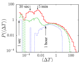
Figure 1: Histogram of average distances between consecutive auctions of the same seller. Full line corresponds to all sellers, dashed line to sellers who initiated at least $10$ auctions, dotted line to sellers who initiated at least $100$ auctions. Time is given in days. The arrows indicate the positions of the features at $\langle\Delta T\rangle=1$ hour, $5$ minutes, $30$ seconds, and the minimum measured value $\langle\Delta T\rangle=1$ sec.

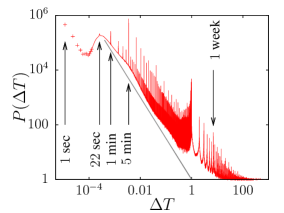
Figure 2: Distribution of distances between consecutive auctions of the same seller. The data are summed for all time series in the data set. The unit of time is one day. The arrows indicate the positions of the maxima at $\Delta T=1$ sec, $22$ secs, $1$ min, $5$ minutes, and $1$ week. The straight line is the power-law dependence $\propto(\Delta T)^{-1.5}$. For $\Delta T>1$ day, the distribution is averaged over intervals $(\Delta T,\Delta T+1\;\mathrm{min})$, in order to see better the structure of peaks at multiples of days.

3 Analysis of the time series

When we analyze the time series of auctions, the first thing to look at is the average density in which the auctions appear. Each seller acts with different mean frequency, so we should ask first, what is the distribution of the average distances between auctions $\langle\Delta T\rangle_{a}=T_{\mathrm{span},a}/(M_{a}-1)$. The results are shown in Fig. 1. We can see that most sellers act at a scale up to $1$ day, with a broad tail extending up to several hundred days, which is about the total extent of our data. So, the tail is to a large extent determined by the finite observation time. The maximum of the distribution lies around $\langle\Delta T\rangle\simeq 5$ minutes and it is not simple, but fairly broad an structured, signaling several types of sellers. So, the set of sellers is very heterogeneous.

However, if we average the distances between auctions over all sellers, we get quite a long time, about $30$ days. This means that the peaks at short distances are somehow not typical. To check this, we looked at what types of sellers constitute these short-distance peaks. We found that mostly they are occasional sellers, who tried to sell a chunk of items within very short time and then they never acted again. Most of them sold at most 10 items. Among about $8000$ sellers characterized by average distance between auctions at most $10$ min, we identified just $13$ intense traders, i. e. those with at least $1000$ auctions. They specialized in several typical branches, like used books (at least $4$ of these $13$ sellers), cosmetics, collectibles (old postcards, fossils, etc.), bijou, and the like. To filter out the occasional sellers, we plot in Fig. 1 also two other histograms, restricted to sellers with at least $10$ and at least $100$ auctions. We can clearly see that the peaks at very small average time distances substantially diminish in the former and vanish in the latter histogram. But still the set of sellers with at least $100$ auctions cover scales of $\langle T\rangle$ starting at $5$ minutes and ending at tens of days. This is a fairly wide range of scales.

When we look at the time series (examples will be shown soon), we observe complex patterns. The first step in understanding the patterns is to see the distribution of the distances between auctions

$$P(\Delta T)=\sum_{a}\sum_{i=1}^{M_{a}-1}\delta\Big{(}T_{a,i+1}-T_{a,i}-\Delta T\Big{)}\;.$$ (1)

(Recall that the time series belongs to a single seller, so the distance is the time which separates the consecutive auctions of the same seller.) The distribution is shown in Fig. 2. We can see large number of sharp peaks at special values of the time distances. However, all of them are artifacts in the sense that they correspond to multiples of natural units of time in which the sellers organize their activity, namely minutes, multiples of $5$ minutes, and especially multiples of days. The non-trivial feature is rather the background decay, over which the peaks are superposed. The data in Fig. 2 suggest that within the time scale of minutes to one day, the background decay is a power law $P(\Delta T)\sim(\Delta T)^{-\gamma}$ with $\gamma\simeq 1.5$.

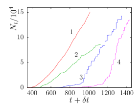
Figure 3: Four typical examples of the time series of activity of sellers on the Aukro site. The numbers $1$ to $4$ refer to corresponding data in Figs. 4 and 5. Time is given in days, day $0$ is 1 January 2009. For better visibility, the time was shifted by the interval $\delta t=0$ for curve $1$, $\delta t=100$ for curve $2$, $\delta t=300$ for curve $3$, and $\delta t=400$ for curve $4$.

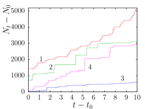
Figure 4: Details of the timeseries shown in Fig. 3, covering $10$ days. The starting day was $t_{0}=750$ for curves $1$, $2$, and $4$, and $t_{0}=970$ for curve $3$. For better visibility, the curves were shifted downwards by $N_{0}=65000$, $47500$, $116200$, and $7600$ for curves $1$, $2$, $3$, and $4$, respectively. Time is given in days.

Let us turn to the analysis of the individual time series now. The overall impression on the time series can be glimpsed from the cumulative number of auctions for one seller up to time $t$, i. e.

$$N_{t,a}=\sum_{i=1}^{M_{a}}\theta(t-T_{i,a})$$ (2)

where $\theta(x)=1$ for $x>0$ and $\theta(x)=0$ elsewhere. We show in Fig. 3 four examples of such time series. We can see that they look rather different. Some of them appear fairly smooth, other exhibit marked steps. Details of the same time series, covering interval of just 10 days is shown in Fig. 4. We can again observe steps at this smaller scale, indicating that a structure close to a fractal is present at least in some of the series. Among several methods of checking the fractality of the series we chose the standard box-counting method, i. e. covering the time span of the series by intervals of variable length.

Let us take one time series, for seller $a$. We fix for a moment a time interval $\Delta t$ and divide the time span $T_{\mathrm{span},a}=T_{\mathrm{max},a}-T_{\mathrm{min},a}$ into non-overlapping intervals of length $\Delta t$. Then, we count the number $N_{\mathrm{occup},a}(\Delta t)$ of such intervals containing at least one auction. Of course, we do that only for $\Delta t<T_{\mathrm{span},a}$.

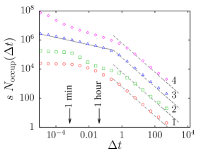
Figure 5: Number of intervals of length $\Delta t$, containing at least one auction, for the timeseries shown in Fig. 3. Time is given in days, arrows showing the scale of one minute and one hour. For better visibility, the data are shifted upwards by a factor $s=1$, $10$, $100$, and $1000$, for curves $1$, $2$, $3$, and $4$, respectively. The straight lines are power dependencies $\propto(\Delta t)^{-0.25}$ (solid line), and $\propto(\Delta t)^{-1}$ (dashed lines).

We can see in Fig. 5 the dependence $N_{\mathrm{occup},a}(\Delta t)$ for the same four examples of time series as shown in Fig 3. (We drop the index $a$ in the axis label, as it bears no information there.) Several regimes can be identified. At times longer than about one day, all the four time series exhibit the behavior $N_{\mathrm{occup}}(\Delta t)\propto(\Delta t)^{-1}$, typical for fractal dimension $\kappa=1$. At shorter time scales, the behavior is much different and non-universal. For example, the time series No. 2 exhibits two shoulders, at $1$ day and at $1$ minute. There is a clear plateau below $1$ minute, showing that at such small scales the fractal dimension is zero. Less clear “plateau” can be seen between $1$ minute and $1$ day, which may perhaps be better characterized as a depression at scale about $1$ hour. This suggests that two typical scales are there. The auctions are put no closer than about $1$ minute, but in bunches extending no more than about one hour. On a scale larger than about one day, the time series looks uniform. This is in marked contrast with time series No. 3 and No 4. At scales shorter than $1$ day, the auctions seem to form a set close to a fractal, more clear for No. 3, with fractal dimension $\kappa\simeq 0.25$, and less clear for No. 4, with slightly larger fractal dimension. The time series No. 1 is yet another type. Again, there are no structures in the time series below the scale of $1$ minute and beyond $1$ day the time series is uniform. However, at the intermediate scales, there is a broad crossover, with neither a clear separation of time scales nor any sign of fractality.

Despite the diversity of the characters of the time series we looked also on their average properties. However, we have to be careful in making the average, for several reasons. First, the time span of the time series varies and so varies the maximum interval $\Delta t$ which enters into the time span. If we averaged directly the number of occupied intervals, we would introduce a systematic error. Therefore, we average the normalized quantity

$$\overline{N_{\mathrm{occup,norm}}(\Delta t)}=\Big{(}\sum_{a}\theta(\Delta t-T_{\mathrm{span},a})\Big{)}^{-1}\sum_{a}\theta(\Delta t-T_{\mathrm{span},a})\frac{N_{\mathrm{occup},a}(\Delta t)}{T_{\mathrm{span},a}}\;.$$ (3)

Second, we found that time sequences with too short time span or containing too few auctions introduce spurious artifacts. Therefore, we limit the sum over $a$ in (3) to such series, for which time span extends more than one week, i. e. $T_{\mathrm{span},a}>7$, and which contain at least $300$ auctions, i. e. $M_{a}\geq 300$.

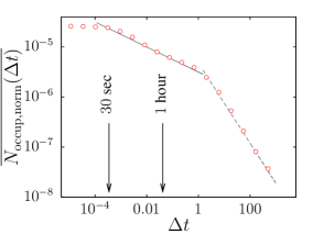
Figure 6: Number of intervals of length $\Delta t$, containing at least one auction, normalized to the time span, and averaged over all timeseries in the data set longer than one week and containing at least $300$ auctions. Time is given in days, arrows showing the scale of one minute and one hour. The straight lines are power dependencies $\propto(\Delta t)^{-0.25}$ (solid line), and $\propto(\Delta t)^{-0.8}$ (dashed line).

The result is shown in Fig. 6. After averaging, three regimes are clearly visible. For the scales below $\Delta t_{1}\simeq 30$ seconds, the fractal dimension is zero on average, indicating that typical time sequences contain no structure at times shorter than $\Delta t_{1}$. Between $\Delta t_{1}$ and the longer scale $\Delta t_{2}\simeq 1$ day, the power-law decay suggests fractal structure with dimension $\kappa\simeq 0.25$. On longer scales than $\Delta t_{2}$, the decay follows a power law with exponent $\kappa\simeq 0.8$, somewhat lower than $1$, showing some non-trivial structure also at longer scales. This result deviates from the data shown in Fig. 5, where all four samples are fitted to $\kappa\simeq 1$ at long time scales, but the deviation is rather small. This indicates that some time series are structured also at larger times, but it is not common.

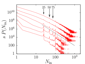
Figure 7: Distribution of number of auctions $N_{\mathrm{in}}$ contained within a time interval $\Delta t$, summed for all time series in the data set. The six curves correspond to intervals (from the bottom to the top) $\Delta t=1$ sec, $10$ sec, $100$ sec, $10^{3}$ sec, $10^{4}$ sec, and $10^{5}$ sec. For better visibility, the data are shifted upwards by the factors (from the bottom to the top) $s=1$, $10$, $100$, $10^{3}$, $10^{4}$, and $10^{5}$. The arrows indicate the positions of $N_{\mathrm{in}}=25$, $50$, and $75$, to stress that these are just the positions of the first peaks. The straight line is the power-law dependence $\propto N_{\mathrm{in}}^{-3}$.

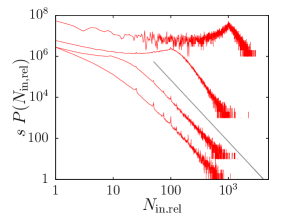
Figure 8: Distribution of number of auctions $N_{\mathrm{in,rel}}$ contained within a time interval $\Delta t=k\langle\Delta T\rangle$, where $\langle\Delta T\rangle$ is the average distance between consecutive auctions in the same time series. The data are summed for all time series in the data set. The four curves correspond to multiples (from the bottom to the top) $k=1$, $10$, $100$ and $1000$. For better visibility, the data are shifted upwards by the factors (from the bottom to the top) $s=1$, $10$, $10^{3}$, and $10^{6}$. The straight line is the power-law dependence $\propto N_{\mathrm{in,rel}}^{-3}$.

The box counting method used above does not reveal all the complexity. A complementary method consists in plotting distribution of number of auctions present within an interval of fixed length. We divide the time span into intervals $(t_{l,a},t_{l+1,a})$, $t_{l,a}=T_{\mathrm{min},a}+l\Delta t$ for $0\leq l<T_{\mathrm{span},a}/\Delta t$ and count

$$P(N_{\mathrm{in}})=\sum_{a}\sum_{k}\delta\Bigg{(}\sum_{i=1}^{M_{a}}\theta(T_{i,a}-t_{l,a})\theta(t_{l+1,a}-T_{i,a})-N_{\mathrm{in}}\Bigg{)}\;.$$ (4)

The results are shown in Fig. 7 for intervals of lengths $\Delta t=10^{n}$ seconds, $n=0,1,2,3,4,5$. We can see that all these interval lengths lead to the same general form of the distribution, with a tail following a power law $P(N_{\mathrm{in}})\sim N_{\mathrm{in}}^{-\tau}$ with exponent $\tau\simeq 3$. However, on top of this background power law, there are significant structures of peaks. The peaks are highest at the shortest interval $\Delta t=1$ sec and they gradually vanish when $\Delta t$ increases. The most interesting fact is that the positions of the peaks are at integer multiples of $25$, the highest ones being at $N_{\mathrm{in}}=25$ and $N_{\mathrm{in}}=100$. This is clearly due to large-scale sellers which place large chunks of auctions at one moment (within one second). More detailed view shows that for $\Delta t=1$ s the peaks at $50$ and $75$ are smaller than those at $25$ and $100$, while for $\Delta t=100$ s these four peaks are of comparable weight, if measured with respect to the background power law, and also the peaks at multiples of $100$ are more pronounced than in the distribution corresponding to $\Delta t=1$ s. This means that there are sellers who put several chunks of sizes $25$, or $100$ not exactly at the same second, but still not farther than about one minute.

In the distribution $P(N_{\mathrm{in}})$, as shown in Fig. 7, we mix sellers who act with different intensity. We have already seen the distribution of the average distances between auctions in Fig. 1. In order to take into account the observed heterogeneity in average distance between auctions, we modify the statistics defined by (4) so that the time span of seller $a$ is divided into intervals of length $\Delta t=k\langle T\rangle_{a}$, i. e. $t_{l,a}=T_{\mathrm{min},a}+lk\langle T\rangle_{a}$. The results are shown in Fig. 8. Again, we can observe the power-law tail with exponent close to $\tau\simeq 3$, but a peak develops at the value $N_{\mathrm{in,rel}}=k$, as should be expected, because $k$ is exactly the average value for the number of auctions within the interval $\Delta t=k\langle T\rangle_{a}$, for every $a$. The exponent of the power-law tail seems to decrease when $k$ increases, but the power-law dependence is still visible. We can conclude that the power-law tail with exponent $\tau\simeq 3$ is due to intrinsic structure of the time series, rather than heterogeneity of the average time scales. Therefore, the noise induced by the activity of the individual agents is itself complex.

4 Conclusions

We performed analysis of complex structure of activity in on-line auctions. For each individual seller, we looked at the time series of the auctions she initiated. The basic, though naturally expected, fact is that the set of sellers is very heterogeneous. The average distance between auctions of the same seller varies from seconds to hundreds of days.

The distribution of distances between subsequent auctions of the same seller exhibits fundamental power-law decay on the scale from $1$ minute to $1$ day, with exponent $\simeq 1.5$. On top of this power-law, there are peaks at natural units of time, like one minute or multiples of $5$ minutes.

We tested the signs of fractality in the time series of auctions. Although each series is unique, the common features can be identified. We must note in advance that the word “fractality” is somewhat abused here, as we always talk on fractal properties within a limited range of scales. By the box counting method, we found that beyond the scale of one day, the series are uniform, i. e. their fractal dimension is $1$. On the other end of the scales, for times shorter than about $30$ seconds the series appears as a set of isolated points, since the measured fractal dimension is $0$. In the intermediate range, from $30$ sec to $1$ day, self-similar structure is observed, with fractal dimension $\simeq 0.25$. Note, however, that these measurements describe averaged properties of the time series, but individual time series may deviate from this mean behavior. Indeed, we observed individual time series with clear fractal shape, and others, in which just two typical scales were observed, without signs of fractality.

From the other side, we found the statistics of number of auctions within an interval of fixed length. This length was either equal for all sellers, or a fixed multiple of average distance between auctions, i. e. different for each seller. In both cases we observed a power-law tail with exponent $\simeq 3$, just the value at the border between Lévy stable and Gaussian distributions. So, the tail is not due to heterogeneity of the set of sellers, but due to the dynamics of each seller separately.

In all the analyses we observed complex patterns of noise in the placement of auctions by individual sellers. There is power-law statistics in the waiting times between actions of the agents, there is power law in the statistics of cumulative activity of an agent over fixed time interval. We may speculate on the consequences of these findings for possible modeling of the behavior of agents in, for example, stock markets. If the agents issued orders to buy or sell shares, rather than placed auctions, the cumulative effect of the power-law distributed numbers of orders would be a power law slowly converging to a Gaussian, which is just the general view of how the statistic of stock market price changes looks like.

Finally, let us mention that similar study of buyer behavior was done. The results seem to be fairly similar, which is probably due to the fact that content and timing of the auctions is entirely in hands of the sellers and the buyers just follow what they could. More subtle differences between the sellers’ and buyers’ side and their possible synchronization will be investigated in a future study.

References

- [1] Alt, R. and Klein, S., Twenty years of electronic markets research - looking backwards towards the future, Electronic Markets, 21 (2011) 41-51.
- [2] Borle, S., Boatwright, P. and Kadane, J. B., The Timing of Bid Placement and Extent of Multiple Bidding: An Empirical Investigation Using eBay Online Auctions, Statistical Science, 21 (2006) 194-205.
- [3] Bouchaud, J.-P. and Potters, M., Theory of Financial Risk and Derivative Pricing (Cambridge University Press, Cambridge, 2003).
- [4] Hou, J. and Blodgett, J., Market structure and quality uncertainty: a theoretical framework for online auction research, Electronic Markets, 20 (2010) 21-32.
- [5] Jank, W. and Yahav, I., E-loyalty networks in online auctions, Annals of Applied Statistics, 4 (2010) 151-178.
- [6] Mantegna, R. N. and Stanley, H. E., Introduction to Econophysics: Correlations and Complexity in Finance (Cambridge University Press, Cambridge, 2000).
- [7] Namazi, A. and Schadschneider, A., Statistical properties of online auctions, International Journal of Modern Physics C, 17 (2006) 1485-1493.
- [8] Papadimitriou, C. and Pierrakos, G., On Optimal Single-Item Auctions, arXiv:1011.1279 (2010).
- [9] Peng, J. and M, H.-G., Distance-based clustering of sparsely observed stochastic processes, with applications to online auctions, Annals of Applied Statistics, 2 (2008) 1056-1077.
- [10] Pigolotti, S., Bernhardsson, S., Juul, J., Galster, G. and Vivo, P., Equilibrium strategy and population-size effects in lowest unique bid auctions, arXiv:1105.0819 (2011).
- [11] Radicchi, F., Baronchelli, A. and Amaral, L. A. N., Rationality, irrationality and escalating behavior in online auctions, arXiv:1105.0469 (2011).
- [12] Reichardt, J. and Bornholdt, S., Clustering of sparse data via network communities - a prototype study of a large online market, J. Stat. Mech., (2007) P06016.
- [13] Shmueli, G., Russo, R. P., Jank, W., The BARISTA: A model for bid arrivals in online auctions, Annals of Applied Statistics, 1 (2007) 412-441.
- [14] Slanina, F. and Konopásek, Z., Eigenvector localization as a tool to study small communities in online social networks, Adv. Compl. Syst., 13 (2010) 699-723.
- [15] Srinivasan, K. and Wang, X., Bidders’ Experience and Learning in Online Auctions: Issues and Implications, Marketing Science, (2010) 988-993.
- [16] Srivastava, A., Motif Analysis in the Amazon Product Co-Purchasing Network, arXiv:1012.4050 (2010).
- [17] Wang, X. and Hu, Y., The effect of experience on Internet auction bidding dynamics, Marketing Letters, 20 (2009) 245-261.
- [18] Yang, I. and Kahng, B., Bidding process in online auctions and winning strategy: Rate equation approach, Phys. Rev. E, 73 (2006) 067101.
- [19] Yang, I., Jeong, H., Kahng, B. and Barabási, A.-L., Emerging behavior in electronic bidding, Phys. Rev. E, 68 (2003) 016102.
- [20] Yang, I., Oh, E. and Kahng, B., Network analysis of online bidding activity, Phys. Rev. E, 74 (2006) 016121.