Differential geometry and scalar gravitational waves

Abstract

Following some strong argumentations of differential geometry in the Landau’s book, some corrections about errors in the old literature on scalar gravitational waves (SGWs) are given and discussed.

In the analysis of the response of interferometers the computation is first performed in the low frequencies approximation, then the analysis is applied to all SGWs in the full frequency and angular dependences.

The presented results are in agreement with the more recent literature on SGWs.

Institute for Theoretical Physics and Mathematics Einstein-Galilei, Via Santa Gonda, 14 - 59100 Prato, Italy

PACS numbers: 04.80.Nn, 04.30.Nk, 04.50.+h

1 Introduction

Second generation interferometric GW detectors, such as Advanced LIGO, are expected to begin operation by 2015 [1]. The realization of a GW astronomy, by giving a significant amount of new information, will be a cornerstone for a better understanding of gravitational physics. In fact, the discovery of GW emission by the compact binary system PSR1913+16, composed by two Neutron Stars [2], has been, for physicists working in this field, the ultimate thrust allowing to reach the extremely sophisticated technology needed for investigating in this field of research. GW astronomy plans to reach sensitivities that will permit to test General Relativity in the dynamical, strong field regime and investigate departures from its predictions, becoming, alternatively, a strong endorsement for Extended Theories like $f(R)$ Theories or Scalar Tensor Gravity [3].

While the response of interferometers to standard tensor GWs in General Relativity has been calculated in lots of works (see for example [3]-[9]), the interaction between interferometers and SGWs arising from Scalar Tensor Gravity is a more recent field of interest and it has not an analogous number of works in the literature. The first work of [10] was improved by the work of the authors of [11]. In [10] the authors did not realize that in their gauge the beam splitter is not left at the origin by the passage of the SGW and furthermore computed a coordinate-time interval than a proper-time interval, reaching the incorrect conclusion that the SGW has longitudinal effect, and does not have transverse one. In [11] the transverse effect of SGWs was shown in the gauge in [10]. After this, in [12], the analysis of [11] was generalized with the computation of the frequency-dependent angular pattern of interferometers in the gauge of [10], while in [11] the angular pattern was only computed in the low frequencies approximation (wavelength much larger than the linear dimensions of the interferometer, under this assumption the amplitude of the SGW, $\Phi$, can be considered ”frozen” at a value $\Phi_{0}$ ).

In this paper the gauge in [10] is re-analysed. Following some strong argumentations on differential geometry in the Landau’s book [13], we show that in [10] there were errors in the geodesic equations of motion too. These errors reflected also in [11] and [12] where incorrect equation of motion taken from [10] were used. Thus, we correct erroneous results which were in three papers published in Physical Review D [10, 11, 12].

In the analysis of the response of interferometers the computation is first made in the low frequencies approximation like in [11], then the calculation is generalized to all SGWs.

At the end of this paper, the correct detector pattern of interferometers in the gauge in [10] is computed. The presented results are in full agreement with the recent ones in [3, 14, 15, 16].

2 A particular gauge for scalar gravitational waves

We consider a gauge which was proposed in the first time in [10]. In this gauge a purely plane SGW is travelling in the $z+$ direction (progressive wave $\Phi\equiv\Phi(t-z)$) and acting on an interferometer whose arms are aligned along the $x$ and $z$ axes [3, 10, 11, 14]). In this gauge it is [10, 11, 14]

$$e_{\mu\nu}^{(s)}=\eta_{\mu\nu}.$$ (1)

Thus, the line element results the conformally flat one (we work with $c=1$ and $\hbar=1$ in this paper)

$$ds^{2}=[1+\Phi(t-z)](-dt^{2}+dz^{2}+dx^{2}+dy^{2}).$$ (2)

Eq. (1) can be rewritten as

$$(\frac{dt}{d\tau})^{2}-(\frac{dx}{d\tau})^{2}-(\frac{dy}{d\tau})^{2}-(\frac{dz}{d\tau})^{2}=\frac{1}{(1+\Phi)},$$ (3)

where $\tau$ is the proper time of the test masses.

From eqs. (2) and (3) the authors of [10] obtained the geodesic equations of motion for test masses (i.e. the beam-splitter and the mirrors of the interferometer), see eq. 3.21, 3.22 and 3.23 of [10],

$$\begin{array}[]{ccc}\frac{d}{d\tau}[(1+\Phi)\frac{dx}{d\tau}]&=&0\\ \\ \frac{d}{d\tau}[(1+\Phi)\frac{dy}{d\tau}]&=&0\\ \\ \frac{d}{d\tau}[(1+\Phi)\frac{dt}{d\tau}]&=&\frac{1}{2}\frac{\partial_{t}(1+\Phi)}{(1+\Phi)}\\ \\ \frac{d}{d\tau}[(1+\Phi)\frac{dz}{d\tau}]&=&-\frac{1}{2}\frac{\partial_{z}(1+\Phi)}{(1+\Phi)}.\end{array}$$ (4)

By using some strong argumentations on differential geometry in the Landau’s book [13], below we will show that eqs. (4) are not correct.

Other incorrect geodesic equations of motion were used in [12], see eqs. 4.2, 4.3, 4.4 and 4.5, in this case for a wave travelling in the $z-$direction (regressive wave). Therefore, the results of [12] and in particular the frequency-dependent angular pattern of eq. (5.25) are not correct.

To derive the correct geodesic equation of motion for a progressive wave, eq. (87,3) in [13], which is

$$\frac{d^{2}x^{i}}{d\tau^{2}}+\Gamma_{kl}^{i}\frac{dx^{k}}{d\tau}\frac{dx^{l}}{d\tau}=0,$$ (5)

can be used.

In this way, using equation (3), one gets

$$\begin{array}[]{ccc}\frac{d^{2}x}{d\tau^{2}}&=&0\\ \\ \frac{d^{2}y}{d\tau^{2}}&=&0\\ \\ \frac{d^{2}t}{d\tau^{2}}&=&\frac{1}{2}\frac{\partial_{t}(1+\Phi)}{(1+\Phi)^{2}}\\ \\ \frac{d^{2}z}{d\tau^{2}}&=&-\frac{1}{2}\frac{\partial_{z}(1+\Phi)}{(1+\Phi)^{2}}.\end{array}$$ (6)

Now, following [13], we show the difference between the correct eqs. (6) and the incorrect ones (4). Let us review the important demonstration in Chapter 10, Paragraph 86 of [13], which implies that the covariant derivative of the metric tensor is equal to zero, i.e. the metric tensor works like a constant in the covariant derivative. Calling $DA_{i}$ the covariant derivative of an arbitrary vector $A_{i}$, it is [13]

$$Du_{i}=g_{ik}Du^{k},$$ (7)

but it is also [13]

$$Du_{i}=D(g_{ik}u^{k})=(Dg_{ik})u^{k}+g_{ik}Du^{k}.$$ (8)

Eqs. (7) and (8) imply

$$Dg_{ik}=0.$$ (9)

On the other hand, eqs. (5) arise from eq. (87,2) in [13], which is

$$Du^{i}=0.$$ (10)

By combining eqs. (10) with eqs. (9) one realizes immediately that the components of the metric tensor, which are all equal to $(1+\Phi)$ in the line element (2), have to be put outside the derivatives in eqs. (4). In other words, eqs. (4) have to be rewritten as

$$\begin{array}[]{ccc}(1+\Phi)\frac{d^{2}x}{d\tau^{2}}&=&0\\ \\ (1+\Phi)\frac{d^{2}y}{d\tau^{2}}&=&0\\ \\ (1+\Phi)\frac{d^{2}t}{d\tau^{2}}&=&\frac{1}{2}\frac{\partial_{t}(1+\Phi)}{(1+\Phi)}\\ \\ (1+\Phi)\frac{d^{2}z}{d\tau^{2}}&=&-\frac{1}{2}\frac{\partial_{z}(1+\Phi)}{(1+\Phi)}.\end{array}$$ (11)

that become

$$\begin{array}[]{ccc}\frac{d^{2}x}{d\tau^{2}}&=&0\\ \\ \frac{d^{2}y}{d\tau^{2}}&=&0\\ \\ \frac{d^{2}t}{d\tau^{2}}&=&\frac{1}{2}\frac{\partial_{t}(1+\Phi)}{(1+\Phi)^{2}}\\ \\ \frac{d^{2}z}{d\tau^{2}}&=&-\frac{1}{2}\frac{\partial_{z}(1+\Phi)}{(1+\Phi)^{2}}.\end{array}$$ (12)

These last equations are exactly eqs. (6).

In [10] the authors did not take in due account the important issue of differential geometry that every component of the metric tensor works like a constant in the covariant derivative. Instead, previous analysis will be fundamental for the conservation of some quantities in the next analysis.

The first and the second of eqs. (6) can be immediately integrated obtaining

$$\frac{dx}{d\tau}=C_{1}=const.$$ (13)

$$\frac{dy}{d\tau}=C_{2}=const.$$ (14)

In this way eq. (3) becomes

$$(\frac{dt}{d\tau})^{2}-(\frac{dz}{d\tau})^{2}=\frac{1}{(1+\Phi)}.$$ (15)

Assuming that test masses are at rest initially it is $C_{1}=C_{2}=0$. Thus, even if the SGW arrives at test masses, there is not motion of test masses within the $x-y$ plane in this gauge.

Now, we show that, in presence of a SGW, there is motion of test masses in the $z$ direction which is the direction of the propagating wave. An analysis of eqs. (6) shows that, to simplify equations, the retarded and advanced time coordinates ($u,v$) can be introduced, exactly like in [10]

$$\begin{array}[]{c}u=t-z\\ \\ v=t+z.\end{array}$$ (16)

From the third and the fourth of eqs. (6) we get

$$\frac{d}{d\tau}\frac{du}{d\tau}=\frac{\partial_{v}[1+\Phi(u)]}{(1+\Phi(u))^{2}}=0.$$ (17)

Equation (17) represents the fundamental difference with the work of [10]. The authors of [10] found the equation (see eq. (3.27) of [10])

$$\frac{d}{d\tau}([1+\Phi(u)]\frac{du}{d\tau})=\frac{\partial_{v}[1+\Phi(u)]}{1+\Phi(u)}=0,$$ (18)

which was integrated obtaining (eq. (3.28) of [10])

$$\frac{du}{d\tau}=\frac{a}{1+\Phi},$$ (19)

while, using eq. (17) we obtain

$$\frac{du}{d\tau}=\alpha,$$ (20)

where $\alpha$ is an integration constant.

From eqs. (15) and (20), it is also

$$\frac{dv}{d\tau}=\frac{\beta}{1+\Phi}$$ (21)

where $\beta\equiv\frac{1}{\alpha}$, and

$$\tau=\beta u+\gamma,$$ (22)

where the integration constant $\gamma$ corresponds simply to the retarded time coordinate translation $u$. Thus, without loss of generality, it can be put equal to zero.

Instead, in [10] the authors found (eq. (3.29) of [10])

$$\frac{dv}{d\tau}=\frac{1}{a}$$ (23)

and (eq. (3.30) of [10])

$$\tau=av+b.$$ (24)

The difference between eqs. (12) and eqs. (4) generates the differences between the incorrect eqs. (3.28) and (3.29) in [10] and the correct eqs. (20) and (21) of this paper, i.e. in our work we obtain the conservation of $\frac{du}{d\tau}$ while the authors of [10] obtained the conservation of $\frac{dv}{d\tau}.$

Now, let us see what is the meaning of the other integration constant $\beta$ (see also [10]). From eqs. (20) and (21) the equation for $z$ can be written as

$$\frac{dz}{d\tau}=\frac{1}{2\beta}(\frac{\beta^{2}}{1+\Phi}-1).$$ (25)

When it is $\Phi=0$ (i.e. before the SGW arrives at the test masses) eq. (25) becomes

$$\frac{dz}{d\tau}=\frac{1}{2\beta}(\beta^{2}-1).$$ (26)

But this is exactly the initial velocity of the test mass, thus $\beta=1$ has to be chosen because test masses are supposed at rest initially. This also imply $\alpha=1$.

To find the motion of a test mass in the $z$ direction, we note that from eq. (22) it is $d\tau=du$, while from eq. (21) it is $dv=\frac{d\tau}{1+\Phi}$.

Because it is also $z=\frac{v-u}{2},$ we obtain

$$dz=\frac{1}{2}(\frac{d\tau}{1+\Phi}-du),$$ (27)

which can be integrated as

$$\begin{array}[]{c}z=z_{0}+\frac{1}{2}\int(\frac{du}{1+\Phi}-du)=\\ \\ =z_{0}-\frac{1}{2}\int_{-\infty}^{t-z}\frac{\Phi(u)}{1+\Phi(u)}du,\end{array}$$ (28)

where $z_{0}$ is the initial position of the test mass.

The displacement of the test mass in the $z$ direction can be written as

$$\begin{array}[]{c}\Delta z=z-z_{0}=-\frac{1}{2}\int_{-\infty}^{t-z_{0}-\Delta z}\frac{\Phi(u)}{1+\Phi(u)}du\\ \\ \simeq-\frac{1}{2}\int_{-\infty}^{t-z_{0}}\frac{\Phi(u)}{1+\Phi(u)}du.\end{array}$$ (29)

The results can be also rewritten in function of the time coordinate $t$:

$$\begin{array}[]{ccc}x(t)&=&x_{0}\\ \\ y(t)&=&y_{0}\\ \\ z(t)&=&z_{0}-\frac{1}{2}\int_{-\infty}^{t-z_{0}}\frac{\Phi(u)}{1+\Phi(u)}d(u)\\ \\ \tau(t)&=&t-z(t),\end{array}$$ (30)

which are different from

$$\begin{array}[]{ccc}x(t)&=&x_{0}\\ \\ y(t)&=&y_{0}\\ \\ z(t)&=&z_{0}+\frac{1}{2}I(t-z(t))\\ \\ \tau(t)&=&t+z(t)\end{array}$$ (31)

with

$$I(t-z(t))\equiv\int_{-\infty}^{t-z_{0}}\Phi(u)du$$ (32)

used from the authors of [11] starting from the incorrect geodesic equations (4).

In [12], for a regressive wave (i.e. in this case it is $\Phi\equiv\Phi(t+z)$), one finds also:

$$\begin{array}[]{ccc}\overline{x}&=&\overline{x}_{i}\\ \\ \overline{y}&=&\overline{y}_{i}\\ \\ \overline{z}&=&\overline{z}_{i}-\frac{1}{2}\int_{-\infty}^{t+\overline{z}_{i}}\delta\Phi(v)d(v)\\ \\ \frac{d\tau}{dv}&=&1+\delta\Phi,\end{array}$$ (33)

see eqs. 4.11 - 4.14, which are incorrect too (note: while in [12] the scalar field is indicated with $\delta\Phi$, and the coordinates are barred, in this paper we use the same notations of [12] only in eq. (33) and (34)). With an analysis analogous to the one used above, it is simple to show that the correct equations of motion for a regressive SGW are

$$\begin{array}[]{ccc}\overline{x}&=&\overline{x}_{i}\\ \\ \overline{y}&=&\overline{y}_{i}\\ \\ \overline{z}&=&\overline{z}_{i}+\frac{1}{2}\int_{-\infty}^{t+\overline{z}_{i}}\frac{\delta\Phi(v)}{1+\delta\Phi(v)}d(v)\\ \\ \tau&=&t+z,\end{array}$$ (34)

Now, let us resume what happens in the gauge (1). We have shown that in the $x-y$ plane an inertial test mass initially at rest remains at rest throughout the entire passage of the SGW, while in the $z$ direction an inertial test mass initially at rest has a motion during the passage of the SGW. Thus, it could appear that SGWs have a longitudinal effect and do not have a transversal one (incorrect conclusion of [10]), but the situation is different as it will be shown in the following analysis.

3 Analysis in the low frequencies approximation

We have to clarify the use of words “at rest”. We want to mean that the coordinates of test masses do not change in the presence of the SGW in the $x-y$ plane, but we will show that the proper distance between the beam-splitter and the mirror of an interferometer changes even though their coordinates remain the same. On the other hand, we will also show that the proper distance between the beam-splitter and the mirror of an interferometer does not change in the $z$ direction even if their coordinates change in the gauge (2).

A good way to analyse variations in the proper distance (time) is by means of “bouncing photons”: a photon can be launched from the beam-splitter to be bounced back by the mirror (see ref. [3, 5, 14] and figure 1).

Figure 1: Photons can be launched from the beam-splitter to be bounced back by the mirror, adapted from ref. [14]

In this section we only deal with the case in which the frequency $f$ of the SGW is much smaller than $\frac{1}{T_{0}}=\frac{1}{L_{0}}$, where $2T_{0}=2L_{0}$ is the total round-trip time of the photon in absence of the SGW, exactly like in [11], but the correct eqs. (30) will be used differently from the authors of [11] that used the incorrect ones (31). The analysis will be generalized to all frequencies in the next section.

Assuming that test masses are located along the $x$ axis and the $z$ axis of the coordinate system the $y$ direction can be neglected because the absence of the $y$ dependence in the metric (2) implies that photon momentum in this direction is conserved [3, 5, 14], and the interval can be rewritten in the form

$$ds^{2}=[1+\Phi(t-z)](-dt^{2}+dx^{2}+dz^{2}).$$ (35)

Let us start by considering the interval for a photon which propagates in the $x$ axis. Photon momentum in the $z$ direction is not conserved, for the $z$ dependence in eq. (2) [3, 5, 14]. Thus, photons launched in the $x$ axis will deflect out of this axis. But this effect can be neglected because the photon deflection into the $z$ direction will be at most of order $\Phi$ [3, 5, 14]. Then, to first order in $\Phi$, the $dz^{2}$ term can be neglected. Thus, from eq. (35) one gets

$$ds^{2}=(1+\Phi)(-dt^{2})+(1+\Phi)dx^{2}.$$ (36)

The condition for null geodesics ($ds^{2}=0$) for photons gives

$$\frac{dx_{photon}}{dt}=\pm 1\Rightarrow x_{photon}=const\pm t.$$ (37)

In the gauge (2) the $x$ coordinates of the beam-splitter and the mirrors are unaffected by the passage of the SGW (see the first of eqs. (30)), then, from eq. (37) one gets that the interval, in coordinate time $t$, that the photon takes for run one round trip in the $x$ arm of the interferometer is

$$T=2L_{0}$$ (38)

(i.e. the photon leaves the beam-splitter at $t=0$ and returns a $t=T$). But this quantity is not invariant under coordinate transformations [3, 5, 14], and we have to work in terms of the beam-splitter proper time which measures the physical length of the arms. In this way, we call $\tau(t)$ and $z_{b}(t)$ the proper time and $z$ coordinate of the beam-splitter at time coordinate $t$ with initial condition $z_{b}(-\infty)=0$. From eqs. (30) it is

$$\begin{array}[]{ccc}z_{b}(t)&=&-\frac{1}{2}\int_{-\infty}^{t-z_{b}(t)}\frac{\Phi(u)}{1+\Phi(u)}du\\ \\ \tau(t)&=t&+\frac{1}{2}\int_{-\infty}^{t-z_{b}(t)}\frac{\Phi(u)}{1+\Phi(u)}du.\end{array}$$ (39)

Thus, calling $\tau_{x}$ the proper time interval that the photon takes to run a round-trip in the $x$ arm, it is

$$\begin{array}[]{c}\tau_{x}=\tau(T)-\tau(0)=T+\frac{1}{2}\int_{-z_{b}(0)}^{t-z_{b}(t)}\frac{\Phi(u)}{1+\Phi(u)}du\simeq\\ \\ \simeq T+\frac{1}{2}\Phi_{0}[T+z_{b}(0)-z_{b}(T)]\simeq\\ \\ \simeq 2L_{0}(1+\frac{1}{2}\Phi_{0}),\end{array}$$ (40)

which is the same result obtained in [11], but here it is obtained from the correct equations of motion.

In the above computation, eq. (38) have been used and, by considering only the first order in $\Phi,$ with $\Phi\ll 1$, the scalar field $\Phi$ has also been considered “frozen” at a fixed value $\Phi_{0}$. Note that $z_{b}(0)-z_{b}(T)$ is second order in $\Phi_{0}$.

The computation of [11] is correct but it starts from incorrect equations of motion, i.e. the authors of [11] casually obtained the correct result (40) starting from incorrect equations of motion. This is because the correct equation of motion (34) for a regressive SGW are casually very similar to the wrong ones (31) for a progressive SGW. In fact, using the notation of [11] and rewriting the correct equations of motion for a regressive wave (34), one gets

$$\begin{array}[]{ccc}x(t)&=&x_{0}\\ \\ y(t)&=&y_{0}\\ \\ z(t)&=&z_{0}+\frac{1}{2}\int_{-\infty}^{t+z_{0}}\frac{\Phi(u)}{1+\Phi(u)}d(u)\\ \\ \tau(t)&=&t+z(t),\end{array}$$ (41)

and, because it is $\Phi(u)\ll 1$ one obtains

$$\frac{\Phi(u)}{1+\Phi(u)}\simeq\Phi(u),$$ (42)

and the only difference between eqs. (41) and eqs. (31) is the different parametrization of the wave: regressive in eq. (41), progressive in eq. (31).

Now, let us consider the $z$ direction: the $x$ direction can be neglected because the absence of the $x$ dependence in the metric (35) implies that photon momentum in this direction is conserved [3, 5, 14]. From eq. (35) it is:

$$ds^{2}=(1+\Phi)(-dt^{2})+(1+\Phi)dz^{2},$$ (43)

and the condition for null geodesics ($ds^{2}=0$) for photons gives

$$\frac{dz_{photon}}{dt}=\pm 1\Rightarrow z_{photon}=const\pm t.$$ (44)

We suppose that the photon leaves the beam splitter at $t=0$; let us ask: how much time does the photon need to arrive at the mirror in the $z$ axis? Calling $T_{1}$ this time one needs the condition

$$z_{b}(0)+T_{1}=z_{m}(T_{1}),$$ (45)

where $z_{m}(t)$ is the $z$ coordinate of the mirror in the $z$ axis at coordinate time $t$ with $z_{m}(-\infty)=L_{0}$. In the same way, when returning from the mirror, the photon arrives again at the beam-splitter at $t=T_{z}=T_{1}+T_{2}$, then

$$z_{m}(T_{1})-T_{2}=z_{b}(T_{z}).$$ (46)

Subtracting eq. (46) from eq. (45) we get

$$T_{z}=T_{1}+T_{2}=[z_{m}(T_{1})-z_{b}(0)]+[z_{m}(T_{1})-z_{b}(T_{z})].$$ (47)

From eq. (30) the equations of motion for $z_{b}$ and $z_{m}$ are:

$$\begin{array}[]{ccc}z_{m}(t)&=&L_{0}-\frac{1}{2}\int_{-\infty}^{t-z_{m}(t)}\frac{\Phi(u)}{1+\Phi(u)}du\\ \\ z_{b}(t)&=&-\frac{1}{2}\int_{-\infty}^{t-z_{b}(t)}\frac{\Phi(u)}{1+\Phi(u)}du,\end{array}$$ (48)

and, substituting them in eq. (47), one obtains

$$T_{z}=2L_{0}-\frac{1}{2}\int_{-z_{b}(0)}^{T_{1}-z_{m}(T_{1})}\frac{\Phi(u)}{1+\Phi(u)}du-\frac{1}{2}\int_{T_{z}-z_{b}(T_{z})}^{T_{1}-z_{m}(T_{1})}\frac{\Phi(u)}{1+\Phi(u)}du.$$ (49)

From eq. (45), the first integral in eq. (49) is zero. The second integral is simple to compute by considering the SGW frozen at a value $\Phi_{0}$. To first order in this value we get

$$\begin{array}[]{c}-\frac{1}{2}\int_{T_{z}-z_{b}(T_{z})}^{T_{1}-z_{m}(T_{1})}\frac{\Phi(u)}{1+\Phi(u)}du\simeq-\frac{1}{2}\Phi_{0}[T_{1}-z_{m}(T_{1})-T_{z}+z_{b}(T_{z})]\simeq\\ \\ \simeq-\frac{1}{2}\Phi_{0}(L_{0}-L_{0}-2L_{0})=+\frac{1}{2}\Phi_{0}2L_{0}.\end{array}$$ (50)

In this way, eq. (49) becomes

$$T_{z}=(1+\frac{1}{2}\Phi_{0})2L_{0}.$$ (51)

Then, calling $\tau_{z}$ the proper time interval that the photon takes to run a round-trip in the $z$ arm, with the same kind of analysis which leaded to eq. (40), we get

$$\begin{array}[]{c}\tau_{z}=\tau(T_{z})-\tau(0)=T_{z}+\frac{1}{2}\int_{-z_{b}(0)}^{t-z_{b}(t)}\frac{\Phi(u)}{1+\Phi(u)}du\simeq\\ \\ \simeq T_{z}+\frac{1}{2}\Phi_{0}[T_{z}+z_{b}(0)-z_{b}(T)]\simeq\\ \\ \simeq T_{z}(1-\frac{1}{2}\Phi_{0})\simeq 2L_{0},\end{array}$$ (52)

which is also the same result of the correspondent equation in [11]:

$$\tau_{z}\simeq T_{z}(1+\frac{1}{2}\Phi_{0})\simeq 2L_{0}.$$ (53)

This is also due to the similarity of eqs. (41) and eqs. (31): the difference in sign between eqs. (52) and (53) is due to the difference between the progressive and the regressive wave. In [11] we find also

$$T_{z}=(1-\frac{1}{2}\Phi_{0})2L_{0},$$ (54)

i.e. a difference in sign with eq. (51), which compensates the difference in sign between eqs. (52) and (53).

Thus, from eqs. (40) and (52) one can say that there is a variation of the proper distance in the $x$ direction (transverse effect of the SGW), while there is not a variation of the proper distance in the $z$ direction (no longitudinal effect).

4 Generalized analysis

Now, let us generalize to all the frequencies the previous result, with an analysis that, with a transform of the time coordinate to the proper time, generalizes to the gauge (1) the analysis of [14]. In this way the response function of the interferometer to SGWs in the gauge (1) will be obtained.

Let us start with the $x$ arm of the interferometer. The condition of null geodesic (37) can be also rewritten as

$$dt^{2}=dx^{2}.$$ (55)

In [3] we used the condition of null geodesic in the case of the transverse-traceless (TT) gauge for tensor waves [18] to obtain the coordinate velocity of the photon which was used for calculations of the photon propagation times between the test masses (eq. (7) in [3]). But from eq. (55) we see that the coordinate velocity of the photon in the gauge (1) is equal to the speed of light. Thus, in this case, the analysis of [3] cannot be used starting directly from the condition of null geodesic. Let us ask which is the important difference between the gauge (1) and the TT gauge for tensor waves analysed in [3]. The answer is that the TT gauge of [3] is a “synchrony gauge”, a coordinate system in which the time coordinate $t$ is exactly the proper time (about the synchrony coordinate system see Cap. (9) of ref. [13]). In the coordinates (2) $t$ is only a time coordinate. The rate $d\tau$ of the proper time is related to the rate $dt$ of the time coordinate from [13]

$$d\tau^{2}=g_{00}dt^{2}.$$ (56)

Only making the time transform (56) the analysis of [3] can be applied to the gauge (1).

From eq. (36) we get $g_{00}=(1+\Phi)$. Then, using eq. (55), one obtains

$$d\tau^{2}=(1+\Phi)dx^{2},$$ (57)

which gives

$$d\tau=\pm(1+\Phi)^{\frac{1}{2}}dx.$$ (58)

Now, we show that the analysis of [3, 5, 14] works in this case too.

From eqs. (30) the coordinates of the beam-splitter $x_{b}=l$ and of the mirror $x_{m}=l+L_{0}$ do not changes under the influence of the SGW in the gauge (2). Hence, the proper duration of the forward trip can be found as

$$\tau_{1}(t)=\int_{l}^{L_{0}+l}[1+\Phi(t)]^{\frac{1}{2}}dx.$$ (59)

To first order in $\Phi$ this integral can be approximated with

$$\tau_{1}(t)=T_{0}+\frac{1}{2}\int_{l}^{L_{0}+l}\Phi(t^{\prime})dx$$ (60)

where

$t^{\prime}=t-(l+L_{0}-x)$.

In the last equation $t^{\prime}$ is the delay time (i.e. $t$ is the time at which the photon arrives in the position $l+L_{0}$, thus $l+L_{0}-x=t-t^{\prime}$ [3, 5, 14]).

In the same way, for the proper duration of the return trip, we write

$$\tau_{2}(t)=T_{0}+\frac{1}{2}\int_{l+L_{0}}^{l}\Phi(t^{\prime})(-dx)$$ (61)

where now

$t^{\prime}=t-(x-l)$

is the delay time and

$T_{0}=L_{0}$

is the transit proper time of the photon in the absence of the SGW, which also corresponds to the transit coordinate time of the photon in the presence of the SGW (see eq. (55)).

Thus, the round-trip proper time will be the sum of $\tau_{2}(t)$ and $\tau_{1}(t-T_{0})$. Then, to first order in $\Phi$, the proper duration of the round-trip will be

$$\tau_{r.t.}(t)=\tau_{1}(t-T_{0})+\tau_{2}(t).$$ (62)

By using eqs. (60) and (61) one immediately gets that deviations of this round-trip proper time (i.e. proper distance) from its unperturbed value are given by

$$\delta\tau(t)=\frac{1}{2}\int_{l}^{L_{0}+l}[\Phi(t-2T_{0}+x-l)+\Phi(t-x+l)]dx.$$ (63)

Eq. (63) generalizes eq. (40) which was derived in the low frequencies approximation. Defining the signal in the arm in the $x$ axis like

$$\frac{\delta\tau(t)}{T_{0}}\equiv\frac{1}{2T_{0}}\int_{l}^{L_{0}+l}[\Phi(t-2T_{0}+x-l)+\Phi(t-x+l)]dx,$$ (64)

the analysis can be translated in the frequency domain using the Fourier transform of the field which is [14]

$$\tilde{\Phi}(\omega)=\int_{-\infty}^{\infty}dt\Phi(t)\exp(i\omega t).$$ (65)

By using definition (65), from eq. (64) we get

$$\frac{\delta\tilde{\tau}(\omega)}{T_{0}}=\Upsilon(\omega)\tilde{\Phi}(\omega),$$ (66)

where $\Upsilon(\omega)$ is the response of the $x$ arm of the interferometer to SGWs [14]:

$$\Upsilon(\omega)=\frac{\exp(2i\omega T_{0})-1}{2i\omega T_{0}}.$$ (67)

Notice that an analysis similar to the one performed in this Section has been used in ref. [3] for tensor waves.

Now, let us see what happens in the $z$ coordinate (see figure 2).

Figure 2: the beam splitter and the mirror are located in the direction of the incoming GW, adapted from ref. [14]

From eq. (43) and the condition $ds^{2}=0$ for null geodesics we get

$$dz=\pm dt.$$ (68)

But, from the last of eqs. (30) the proper time is

$$d\tau(t)=dt-dz,$$ (69)

and, combining eq. (68) with eq. (69), one obtains

$$d\tau(t)=dt\mp dt.$$ (70)

Hence

$$\tau_{1}(t)=0$$ (71)

for the forward trip

and

$$\tau_{2}(t)=\int_{0}^{T_{0}}2dt=2T_{0}$$ (72)

for the return trip. At the end we get

$$\tau(t)=\tau_{1}(t)+\tau_{2}(t)=2T_{0}.$$ (73)

Thus, it is $\delta\tau=\delta L_{0}=0$, i.e. there is no longitudinal effect. This is a direct consequence of the fact that a SGW propagates at the speed of light. In this way in the forward trip the photon travels at the same speed of the SGW and its proper time is equal to zero (eq. (71)), while in the return trip the photon travels against the SGW and its proper time redoubles (eq. (72)).

5 The detector pattern

As the arms of an interferometer are in general in the $\overrightarrow{u}$ and $\overrightarrow{v}$ directions, to compute the line element in the $\overrightarrow{u}$ and $\overrightarrow{v}$ directions, a spatial rotation of the coordinates (2) is needed:

$$\begin{array}[]{ccc}u&=&-x\cos\theta\cos\phi+y\sin\phi+z\sin\theta\cos\phi\\ \\ v&=&-x\cos\theta\sin\phi-y\cos\phi+z\sin\theta\sin\phi\\ \\ w&=&x\sin\theta+z\cos\theta,\end{array}$$ (74)

or, in terms of the $x,y,z$ frame:

$$\begin{array}[]{ccc}x&=&-u\cos\theta\cos\phi-v\cos\theta\sin\phi+w\sin\theta\\ \\ y&=&u\sin\phi-v\cos\phi\\ \\ z&=&u\sin\theta\cos\phi+v\sin\theta\sin\phi+w\cos\theta.\end{array}$$ (75)

In this way, the SGW is propagating from an arbitrary direction $\overrightarrow{r}$ to the interferometer (see figure 3).

Figure 3: a SGW incoming from an arbitrary direction, adapted from ref. [14]

The metric tensor transforms like (see Chap. (10) of ref. [13]):

$$g^{ik}=\frac{\partial x^{i}}{\partial x^{\prime l}}\frac{\partial x^{k}}{\partial x^{\prime m}}g^{\prime lm}.$$ (76)

Using eq. (74), eq. (75) and eq. (76), in the new rotated frame, the line element (2) in the $\overrightarrow{u}$ direction becomes (here one can neglect the $v$ and $w$ directions because bouncing photons will be used and the photon deflection into the $v$ and $w$ directions will be at most of order $\Phi,$ then, to first order in $\Phi$, the $dv^{2}$ and $dw^{2}$ terms can be neglected [14]):

$$ds^{2}=[1+(1-\sin^{2}\theta\cos^{2}\phi)\Phi(t-u\sin\theta\cos\phi)](du^{2}-dt^{2}).$$ (77)

Considering a photon launched from the beam-splitter to be bounced back by the mirror, the condition for null geodesics ($ds^{2}=0$) in eq. (77) gives

$$du^{2}=dt^{2}.$$ (78)

Thus, also in this case, the analysis of [3] cannot be used starting directly from the condition of null geodesic. But a generalization of previous analysis can be used. In fact, also the metric (77) is not a “synchrony coordinate system”, thus, also in this line element, $t$ is only a time coordinate. The rate $d\tau$ of the proper time is related to the rate $dt$ of the time coordinate from eq. (56).

From eq. (77) we get

$$g_{00}=[1+(1-\sin^{2}\theta\cos^{2}\phi)\Phi(t-u\sin\theta\cos\phi)].$$ (79)

.

Then, using eq. (78), we obtain

$$d\tau^{2}=[1+(1-\sin^{2}\theta\cos^{2}\phi)\Phi(t-u\sin\theta\cos\phi)]du^{2}$$ (80)

which gives

$$d\tau=\pm[1+(1-\sin^{2}\theta\cos^{2}\phi)\Phi(t-u\sin\theta\cos\phi)]{}^{\frac{1}{2}}du.$$ (81)

We put the beam splitter in the origin of the new coordinate system (i.e. $u_{b}=0$, $v_{b}=0$, $w_{b}=0$). From eqs. (30) one gets that an inertial test mass initially at rest in the $x-y$ plane of the coordinates (2), remains at rest throughout the entire passage of the SGW. We also know that the coordinates of the beam-splitter and of the mirror change under the influence of the SGW in the $z$ direction, but this fact does not influence the total variation of the round trip proper time of the photon (eq. (73)). Then, in the computation of the variation of the proper distance in the gauge (2), the coordinates of the beam-splitter $u_{b}=0$ and of the mirror $u_{m}=L_{0}$ can be considered fixed even in the $u-v$ plane, because the rotation (74) does not change the situation. Thus, the proper duration of the forward trip can be found as

$$\tau_{1}(t)=\int_{0}^{L_{0}}[1+(1-\sin^{2}\theta\cos^{2}\phi)\Phi(t-u\sin\theta\cos\phi)]{}^{\frac{1}{2}}du$$ (82)

with

$t^{\prime}=t-(L_{0}-u)$.

In the last equation $t^{\prime}$ is the delay time (see Section 4).

To first order in $\Phi$ this integral is well approximated with

$$\tau_{1}(t)=T_{0}+\frac{1-\sin^{2}\theta\cos^{2}\phi}{2}\int_{0}^{L_{0}}\Phi(t^{\prime}-u\sin\theta\cos\phi)du,$$ (83)

where

$T_{0}=L_{0}$

is the transit time of the photon in the absence of the SGW. Similarly, the duration of the return trip will be

$$\tau_{2}(t)=T_{0}+\frac{1-\sin^{2}\theta\cos^{2}\phi}{2}\int_{L_{0}}^{0}\Phi(t^{\prime}-u\sin\theta\cos\phi)(-du),$$ (84)

though now the delay time is

$t^{\prime}=t-(u-l)$.

The round-trip time will be the sum of $\tau_{2}(t)$ and $\tau_{1}[t-T_{0}]$. Thus, to first order in $\Phi$, the proper duration of the round-trip will be

$$\tau_{r.t.}(t)=\tau_{1}[t-T_{0}]+\tau_{2}(t).$$ (85)

Using eqs. (83) and (84) one immediately gets that deviations of this round-trip time (i.e. proper distance) from its unperturbed value are given by

$$\begin{array}[]{c}\delta\tau(t)=\frac{1-\sin^{2}\theta\cos^{2}\phi}{2}\int_{0}^{L_{0}}[\Phi(t-2L_{0}+u(1-\sin\theta\cos\phi))+\\ \\ +\Phi(t-u(1+\sin\theta\cos\phi))]du.\end{array}$$ (86)

By using the Fourier transform of the scalar field defined by eq. (65), in the frequency domain it is:

$$\delta\tilde{\tau}(\omega)=(1-\sin^{2}\theta\cos^{2}\phi)\tilde{H}_{u}(\omega,\theta,\phi)\Phi(\omega)$$ (87)

where

$$\begin{array}[]{c}\tilde{H}_{u}(\omega,\theta,\phi)=\frac{-1+\exp(2i\omega L_{0})}{2i\omega(1-\sin^{2}\theta\cos^{2}\phi)}+\\ \\ +\frac{\sin\theta\cos\phi((1+\exp(2i\omega L_{0})-2\exp i\omega L_{0}(1+\sin\theta\cos\phi)))}{2i\omega(1-\sin^{2}\theta\cos^{2}\phi)},\end{array}$$ (88)

and one immediately obtains that $\tilde{H}_{u}(\omega,\theta,\phi)\rightarrow L_{0}$ when $\omega\rightarrow 0$.

Thus, the total response function of the arm of the interferometer in the $\overrightarrow{u}$ direction to the SGW is:

$$\Upsilon_{u}^{SGW}(\omega)=\frac{1-\sin^{2}\theta\cos^{2}\phi}{L_{0}}\tilde{H}_{u}(\omega,\theta,\phi).$$ (89)

In the same way, the line element (2) in the $\overrightarrow{v}$ direction becomes:

$$ds^{2}=[1+(1-\sin^{2}\theta\sin^{2}\phi-)\Phi(t-v\sin\theta\sin\phi)](dv^{2}-dt^{2}),$$ (90)

and, with the same kind of analysis used for the $\overrightarrow{u}$ direction, the response function of the $\overrightarrow{v}$ arm of the interferometer to the SGW results:

$$\Upsilon_{v}^{SGW}=\frac{1-\sin^{2}\theta\sin^{2}\phi}{L_{0}}\tilde{H}_{v}(\omega,\theta,\phi),$$ (91)

where

$$\begin{array}[]{c}\tilde{H}_{v}(\omega,\theta,\phi)=\frac{-1+\exp(2i\omega L_{0})}{2i\omega(1-\sin^{2}\theta\sin^{2}\phi)}+\\ \\ +\frac{\sin\theta\sin\phi((1+\exp(2i\omega L_{0})-2\exp i\omega L(1+\sin\theta\sin\phi)))}{2i\omega(1-\sin^{2}\theta\sin^{2}\phi)},\end{array}$$ (92)

and we see that also $\tilde{H}_{v}(\omega,\theta,\phi)\rightarrow L_{0}$ when $\omega\rightarrow 0$.

Then, the detector pattern of an interferometer to the SGW is:

$$\begin{array}[]{c}\tilde{H}^{SGW}(\omega)=\frac{1-\sin^{2}\theta\cos^{2}\phi}{L_{0}}\tilde{H}_{u}(\omega,\theta,\phi)-\frac{1-\sin^{2}\theta\sin^{2}\phi}{L_{0}}\tilde{H}_{v}(\omega,\theta,\phi)=\\ \\ =\frac{\sin\theta}{2i\omega L}\{\cos\phi[1+\exp(2i\omega L)-2\exp i\omega L(1+\sin\theta\cos\phi)]+\\ \\ -\sin\phi[1+\exp(2i\omega L_{0})-2\exp i\omega L_{0}(\sin\theta\sin\phi-1)]\},\end{array}$$ (93)

that is exactly the detector pattern of eq. (150) of [14], where the computation was made in the TT gauge, and the same result of eq. (18) of [19], where this response function has been used to analyse the cross-correlation between the Virgo interferometer and the MiniGRAIL resonant sphere for the detection of SGWs.

For a sake of clearness, the derivation of this detector pattern in the TT gauge will be sketch in the appendix [17].

In the low frequencies limit ($\omega\rightarrow 0$) eq. (93) is also in perfect agreement with the detector pattern of eq. (15) of [11], and also with the low frequencies detector pattern of [15, 16]:

$$\tilde{H}^{SGW}(\omega\rightarrow 0)=-\sin^{2}\theta\cos 2\phi.$$ (94)

The detector pattern of eq. (93) is different from the one in eq. (5.25) of [12], because in [12] the computation was made starting from incorrect equations of motion. The similarity between the two detector patterns is due to the fact that the correct equations of motion (30) for a progressive SGW are casually very similar to the incorrect ones (33) for a regressive SGW used in [12] (see also comments in Section 3 about the casual similarity between wrong and correct equations of motion).

Notice that also in this case an analysis similar to the one performed in this Section has been used in ref. [3] for tensor waves.

The absolute value of the total response function of the Virgo interferometer ($L=3$ Km) for SGWs with $\theta=\frac{\pi}{4}$ and $\phi=\frac{\pi}{3}$ and the angular dependence of the response of the Virgo interferometer for a SGW with a frequency of $f=100Hz$ are respectively shown in figs. 4 and 5.

Figure 4: the absolute value of the total response function of the Virgo interferometer to SGWs for $\theta=\frac{\pi}{4}$ and $\phi=\frac{\pi}{3}$, adapted from ref. [14]

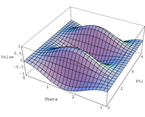
Figure 5: the angular dependence of the response of the Virgo interferometer for a SGW with a frequency of $f=100Hz$, adapted from ref. [14]

6 Conclusions

Following some ideas in the Landau’s book, some corrections about errors in the old literature on SGWs have been released and discussed. In the analysis of the response of interferometers the computation has been first performed in the low frequencies approximation. After this, the analysis has been applied to all SGWs in the full frequency and angular dependences.

The presented results are in agreement with the more recent literature on SGWs.

Appendix

For a sake of completeness, let us sketch the derivation of the detector pattern (93) in the TT gauge. We emphasize that hereafter we closely follow the papers [14, 19].

The TT gauge can be extended to SGWs in Scalar Tensor Gravity too [3, 11, 14, 19]. In the TT gauge, for a purely massless SGW propagating in the positive $z$ direction, with the interferometer located at the origin of the coordinate system with arms in the $\overrightarrow{x}$ and $\overrightarrow{y}$ directions, the metric perturbation is given by [3, 11, 14, 19]

$$h_{\mu\nu}(t-z)=\Phi(t-z)e_{\mu\nu}^{(s)},$$ (95)

where $\Phi\ll 1$, $e_{\mu\nu}^{(s)}\equiv diag(0,1,1,0)$, and the line element is

$$ds^{2}=-dt^{2}+dz^{2}+[1+\Phi(t-z)][dx^{2}+dy^{2}].$$ (96)

To compute the response function for an arbitrary propagating direction of the SGW one recalls that the arms of the interferometer are in the $\overrightarrow{u}$ and $\overrightarrow{v}$ directions, while the $x,y,z$ frame of (96) is adapted to the propagating SGW. Thus, the spatial rotations of the coordinate system (74) and (75) are needed. In this way the SGW is propagating from an arbitrary direction to the interferometer (see figure 3). The beam splitter is also put in the origin of the new coordinate system (i.e. $u_{b}=0$, $v_{b}=0$). By using eq. (74), eq. (75) and eq. (76), the line element (96) in the $\overrightarrow{u}$ direction becomes:

$$ds^{2}=-dt^{2}+[1+(1-\sin^{2}\theta\cos^{2}\phi)\Phi(t-u\sin\theta\cos\phi)]du^{2}.$$ (97)

In this case, by applying the condition for null geodesics ($ds^{2}=0$) in eq. (97) one gets immediately eq. (80) because in the TT gauge the coordinate time is exactly the proper time. In the same way, the line element (96) in the $\overrightarrow{v}$ direction becomes:

$$ds^{2}=-dt^{2}+[1+(1-\sin^{2}\theta\sin^{2}\phi)\Phi(t-v\sin\theta\sin\phi)]dv^{2}.$$ (98)

At this point, one can perform in detail exactly the same analysis in section 5 in order to obtain the detector pattern (93).

References

• [1] The LIGO Scientific Collaboration: B. Abbott, et al., Rept. Prog. Phys. 72, 076901 (2009).
• [2] R. A. Hulse and J.H. Taylor, Astrophys. J. Lett. 195, 151 (1975).
• [3] C. Corda, Int. Journ. Mod. Phys. D, 18, 14, 2275-2282 (2009, Honorable Mention Gravity Research Foundation).
• [4] P. Saulson, Fundamental of Interferometric Gravitational Waves Detectors, World Scientific, Singapore (1994).
• [5] M. Rakhmanov, Phys. Rev. D 71, 084003 (2005).
• [6] L. P. Grishchuk, Sov. Phys. JETP 39, 402 (1974).
• [7] F. B. Estabrook and H. D. Wahlquist, Gen. Relativ. Gravit. 6, 439 (1975).
• [8] M. Tinto, F.B. Estabrook and J. W. Armstrong, Phys. Rev. D 65, 084003 (2002).
• [9] K.S. Thorne KS, Proc. Snowmass’94 Summer Study On Particle and Nuclear Astrophysics and Cosmology - Ed. E. W. Kolb and R. Peccei - World Scientific, Singapore, p. 398 (1995).
• [10] M. Shibata, K. Nakao and T. Nakamura, Phys. Rev. D 50, 7304 (1994).
• [11] M. Maggiore and A. Nicolis, Phys. Rev. D 62 024004 (2000).
• [12] K. Nakao, T. Harada, M. Shibata, S. Kawamura and T. Nakamura, Phys. Rev. D 63, 082001 (2001).
• [13] L. D. Landau and E. M. Lifshitz, Classical Theory of Fields (3rd ed.), London: Pergamon. ISBN 0-08-016019-0. Vol. 2 of the Course of Theoretical Physics. (1971).
• [14] S. Capozziello and C. Corda, Int. J. Mod. Phys. D 15, 1119 -1150 (2006).
• [15] N. Bonasia N and M. Gasperini, Phys. Rew. D, 71 104020 (2005).
• [16] M. E. Tobar, T. Suzuki and K. Kuroda, Phys. Rev. D 59, 102002 (1999).
• [17] Private communication Maria Felicia De Laurentis of the Naples University.
• [18] C. W. Misner, K. S. Thorne and J. A. Wheeler , β€œGravitation” , W. H. Feeman and Company -(1973=
• [19] C. Corda, Mod. Phys. Lett. A 22, 23, 1727–1735 (2007).