Exact Bayesian Inference for the Bingham Distribution

Abstract

This paper is concerned with making Bayesian inference from data that are assumed to be drawn from a Bingham distribution. A barrier to the Bayesian approach is the parameter-dependent normalising constant of the Bingham distribution, which, even when it can be evaluated or accurately approximated, would have to be calculated at each iteration of an MCMC scheme, thereby greatly increasing the computational burden. We propose a method which enables exact (in Monte Carlo sense) Bayesian inference for the unknown parameters of the Bingham distribution by completely avoiding the need to evaluate this constant. We apply the method to simulated and real data, and illustrate that it is simpler to implement, faster, and performs better than an alternative algorithm that has recently been proposed in the literature

.

1 Introduction

Observations that inherit a direction occur in many scientific disciplines (see, for example, Mardia and Jupp, 2000). For example, directional data arise naturally in the biomedical field for protein structure (Boomsma et al., 2008), cell–cycle (Rueda et al., 2009) and circadian clock experiments (Levine et al., 2002); see also the references in Ehler and Galanis (2011). A distribution that has proved useful as a model for spherical data which arise as unsigned directions is the Bingham distribution (Bingham, 1974; Mardia and Jupp, 2000).

The Bingham distribution can be constructed by conditioning a zero-mean multivariate Normal (MVN) distribution to lie on the sphere $\mathcal{S}^{q-1}$ of unit radius in $\mathbb{R}^{q}$. In particular, for a given matrix $A$ of dimension $q\times q$, the density with respect to the uniform measure on $\mathcal{S}^{q-1}$ is given by

$$f({\bm{x}};A)=\frac{\exp{(-{\bm{x}}^{T}A{\bm{x}})}}{c(A)},\quad{\bm{x}}^{T}{\bm{x}}=1\mbox{ and }{\bm{x}}\in\mathbb{R}^{q},$$ (1)

where $c(A)$ is the corresponding normalising constant.

Having observed some directional data, interest then lies in inference for the matrix $A$ in (1). The likelihood of the observed data given the parameters can easily be written down and at first glance it appears that maximum likelihood inference for $A$ is straightforward. However, inferring the matrix $A$ is rather challenging. That is due to the fact that the likelihood of the observed data given the matrix $A$ involves the parameter-dependent normalising constant $c(A)$ which, in the general case, is not available in closed form. Therefore this poses significant challenges to undertake statistical inference involving the Bingham distribution either in a frequentist or Bayesian setting.

Although a maximum likelihood estimator for $A$ can be derived by iterative techniques which are based on being able to approximate $c(A)$ (see, for example, Kent, 1987; Kume and Wood, 2005, 2007; Sei and Kume, 2013), very little attention has been drawn in the literature concerning estimation of $A$ within a Bayesian framework. Walker (2013) considered Bayesian inference for the Bingham distribution which removes the need to compute the normalising constant, using a (more general) method that was developed earlier (Walker, 2011) and cleverly gets around the intractable nature of the normalising constant. However, it requires the introduction of several latent variables and a Reversible-Jump Markov Chain Monte Carlo (RJMCMC) sampling scheme.

The main contribution of this paper is to show how one can draw Bayesian inference for the matrix $A$, by exploiting the recent developments in Bayesian computation for distributions with doubly intractable normalising constants (Møller et al., 2006; Murray et al., 2006). The main advantage of our approach is that it does not require any numerical approximation to $c(A)$ and hence, enables exact (in the Monte Carlo sense) Bayesian inference for $A$. Our method relies on being able to simulate exact samples from the Bingham distribution which can be done by employing an efficient rejection sampling algorithm proposed by Kent and Ganeiber (2012).

The rest of the paper is structured as follows. In Section 2 we introduce the family of Angular Central Gaussian distributions and illustrate how such distributions serve as efficient proposal densities to sample from the Bingham distribution. In Section 3 we describe our proposed algorithm while in Section 4 we illustrate our method both using simulated and real directional data from earthquakes in New Zealand. In Section 5 we discuss the computational aspects of our method as well as directions for future research.

2 Rejection Sampling

2.1 Preliminaries

Rejection sampling (Ripley, 1987) is a method for drawing independent samples from a distribution with probability density function $f(x)=f^{*}(x)/Z_{f}$ assuming that we can evaluate $f^{*}(x)$ for any value $x$, but may not necessarily know $Z_{f}$. Suppose that there exists another distribution, with probability density function $g(x)=g^{*}(x)/Z_{g}$, often termed an envelope density, from which we can easily draw independent samples and can evaluate $g^{*}(x)$ at any value $x$. We further assume that there exists a constant $M^{*}$ for which $M^{*}g^{*}(x)\geq f^{*}(x)$ $\forall x$. We can then draw samples from $f(x)$ as follows:

1. Draw a candidate value $y$ from $g(x)$ and $u$ from $U(0,1)$;

2. if $u\leq\frac{f^{*}(y)}{M^{*}g^{*}(y)}$ accept $y$; otherwise reject $y$ and go to step 1.

The set of accepted points provides a sample from the target density $f(x)$. It can be shown that the number of trials until a candidate is accepted has a geometric distribution with mean $M$, where

$$M=\sup_{x\in\mathcal{R}}\left\{\frac{f(x)}{g(x)}\right\}<\infty.$$ (2)

Therefore, the algorithm will work efficiently provided that $M$ is small or, in other words, the probability of acceptance $(1/M)$ is large. Moreover, it is important to note that it is not necessary to know the normalising constants $Z_{f}$ and $Z_{g}$ to implement the algorithm; the only requirement is being able to draw from the envelope density $g(x)$ and knowledge of $M^{*}$ (rather than $M$).

2.2 The Angular Central Gaussian Distribution

The family of the angular central Gaussian(ACG) distributions is an alternative to the family of the Bingham distributions for modelling antipodal symmetric directional data (Tyler, 1987). An angular central Gaussian distribution on the $(q-1)-$dimensional sphere $\mathcal{S}^{q-1}$ can be obtained by projecting a multivariate Gaussian distribution in $\mathbb{R}^{q}$, $q\geq 2$, with mean zero onto $\mathcal{S}^{q-1}$ with radius one. In other words, if the vector ${\bm{y}}$ has a multivariate Normal distribution in $\mathbb{R}^{q}$ with mean ${\bm{0}}$ and variance covariance matrix $\Psi$, then the vector ${\bm{x}}={\bm{y}}/||{\bm{y}}||$ follows an ACG distribution on $\mathcal{S}^{q-1}$ with $q\times q$ symmetric positive$-$definite parameter matrix $\Psi$ (Mardia and Jupp, 2000). The probability density function of the ACG distribution with respect to the surface measure on $\mathcal{S}^{q-1}$ is given by

$$g({\bm{x}};\Psi)=w_{q}^{-1}|\Psi|^{-1/2}\left({\bm{x}}^{T}\Psi^{-1}{\bm{x}}\right)^{-q/2}=c_{\mathrm{ACG}}(\Psi)g^{*}({\bm{x}};\Psi)$$ (3)

where the constant $w_{q}=2\pi^{q/2}/\Gamma(q/2)$ represents the surface area on $\mathcal{S}^{q-1}$. Denote by $c_{\mathrm{ACG}}(\Psi)=w_{q}^{-1}|\Psi|^{-1/2}$ the normalising constant where $\Psi$ is a $q\times q$ symmetric positive$-$definite matrix.

2.3 Rejection Sampling for the Bingham Distribution

Kent and Ganeiber (2012) have demonstrated that one can draw samples from the Bingham distribution using the ACG distribution as an envelope density within a rejection sampling framework. In particular, the following algorithm can be used to simulate a value from the Bingham distribution with parameter matrix $A$:

1. Set $\Psi^{-1}=I_{q}+\frac{2}{b}A$ and $M^{*}\geq\sup_{\bm{x}}\left\{\frac{f*(x)}{g*(x)}\right\};$

2. draw $u$ from $U(0,1)$ and a candidate value ${\bm{y}}$ from the ACG distribution on the sphere with parameter matrix $\Psi$;

3. if $u<\frac{f^{*}({\bm{y}};A)}{M^{*}g^{*}({\bm{y}};\Psi)}$ accept ${\bm{y}}$; otherwise reject ${\bm{y}}$ and go to Step 1.

Here, $f^{*}(\bm{y};A)=\exp(-\bm{y}^{T}A\bm{y})$, and $g^{*}(\bm{y};\Psi)=(\bm{y}^{T}\Psi^{-1}\bm{y})^{-\frac{q}{2}}$, the unnormalized Bingham and ACG densities respectively, and $b<q$ is a tuning constant. We found that setting $b=1$ as a default works well in many situations, but an optimal value can be found numerically by maximising the acceptance probability $1/M$ (see, for example, Ganeiber, 2012).

3 Bayesian Inference

3.1 Preliminaries

Consider the probability density function of the Bingham distribution as given in (1). If $A=V\Lambda V^{T}$ is the Singular Value Decomposition of $A$ where $V$ is orthogonal and $\Lambda=\mbox{diag}(\lambda_{1},\ldots,\lambda_{q})$, then it can be shown that if ${\bm{x}}$ is drawn from a distribution with probability density function $f({\bm{x}};A)$, the corresponding random vector ${\bm{y}}=X^{T}V$ is drawn from a distribution with density $f({\bm{x}};\Lambda)$ (see, for example, Kume and Walker, 2006; Kume and Wood, 2007). Therefore, without loss of generality, we assume that $A=\Lambda=\mbox{diag}(\lambda_{1},\ldots,\lambda_{q})$. Moreover, to ensure identifiability, we assume that $\lambda_{1}\geq\lambda_{2}\geq\ldots\lambda_{q}=0$ (Kent, 1987). Therefore, the probability density function becomes

$$f({\bm{x}};\Lambda)=\frac{\exp\left\{-\sum_{i=1}^{q-1}\lambda_{i}x_{i}^{2}\right\}}{c(\Lambda)}$$ (4)

with respect to a uniform measure on the sphere and

$$c(\Lambda)=\int_{{\bm{x}}\in S^{q-1}}\exp\left\{-\sum_{i=1}^{q-1}\lambda_{i}x_{i}^{2}\right\}\mbox{ d}S^{q-1}({\bm{x}}).$$

Suppose $({{\bm{x}}_{1},{\bm{x}}_{2},\ldots,{\bm{x}}_{n}})$ is a sample of unit vectors in $\mathcal{S}^{q-1}$ from the Bingham distribution with density (4). Then the likelihood function is given by

$$L(\Lambda)=\frac{1}{c(\Lambda)^{n}}\exp\left\{-\sum_{i=1}^{q-1}\lambda_{i}\sum_{j=1}^{n}\left(x_{j}^{i}\right)^{2}\right\}=\frac{1}{c(\Lambda)^{n}}\exp\left\{-n\sum_{i=1}^{q-1}\lambda_{i}\tau_{i}\right\},$$ (5)

where $\tau_{i}=\frac{1}{n}\sum_{i=1}^{n}\left(x_{j}^{i}\right)^{2}$. The data can therefore be summarised by $(n,\tau_{1},\ldots,\tau_{q-1})$, and $(\tau_{1},\ldots,\tau_{q-1})$ are sufficient statistics for $(\lambda_{1},\ldots,\lambda_{q-1})$.

3.2 Bayesian Inference

We are interested in drawing Bayesian inference for the matrix $\Lambda$, or equivalently, for ${\bm{\lambda}}=(\lambda_{1},\ldots,\lambda_{q-1})$. The likelihood function in (5) reveals that the normalising constant $c(\Lambda)$ plays a crucial role. The fact that there does not exist a closed form expression for $c(\Lambda)$ makes Bayesian inference for $\Lambda$ very challenging.

For example, if we assign independent Exponential prior distributions to the elements of ${\bm{\lambda}}$ with rate $\mu_{i}$ (i.e. mean $1/\mu_{i}$) subject to the constraint that $\lambda_{1}\geq\lambda_{2}\geq\ldots\geq\lambda_{q-1}$ then the density of the posterior distribution of $\Lambda$ up to proportionality given the data is as follows:

$$\pi({\bm{\lambda}}|{\bm{x}}_{1},\ldots,{\bm{x}}_{n}) \propto L(\Lambda)\prod_{i=1}^{q-1}\exp\{-\lambda_{i}\mu_{i}\}\cdot{\bm{1}}\left(\lambda_{1}\geq\lambda_{2}\geq\ldots\geq\lambda_{q-1}\right)$$ (6)

$$= \frac{1}{c(\Lambda)^{n}}\exp\left\{-\sum_{i=1}^{q-1}\lambda_{i}(n\tau_{i}+\mu_{i})\right\}\cdot{\bm{1}}\left(\lambda_{1}\geq\lambda_{2}\geq\ldots\geq\lambda_{q-1}\right).$$

Consider the following Metropolis-Hastings algorithm which aims to draw samples from $\pi({\bm{\lambda}}|{\bm{x}}_{1},\ldots,{\bm{x}}_{n})$:

1. Suppose that the current state of the chain is ${\bm{\lambda}}^{\mbox{cur}}$;

2. Update ${\bm{\lambda}}$ using, for example, a random walk Metropolis step by
   proposing ${\bm{\lambda}}^{\mbox{can}}\sim N_{q-1}\left({\bm{\lambda}}^{\mbox{cur}},\Sigma\right)$;

3. Repeat steps 1-2.

Note that $N_{q-1}\left({\bm{m}},S\right)$ denotes the density of a multivariate Normal distribution with mean vector ${\bm{m}}$ and variance-covariance matrix $S$. Step 2 of the above algorithm requires the evaluation of the ratio $\pi\left({\bm{\lambda}}^{\mbox{can}}|{{\bm{x}}_{1},\ldots,{\bm{x}}_{n}}\right)/\pi\left({\bm{\lambda}}^{\mbox{cur}}|{{\bm{x}}_{1},\ldots,{\bm{x}}_{n}}\right)$, which in turn involves evaluation of the ratio $c(\Lambda^{\mbox{can}})/c(\Lambda^{\mbox{cur}})$. Therefore, implementing the above algorithm requires an approximation of the normalising constant. In principle, one can employ one of the proposed methods in the literature which are based either on asymptotic expansions (Kent, 1987), saddlepoint approximations (Kume and Wood, 2005) or holonomic gradient methods (Sei and Kume, 2013). Although such an approach is feasible, in practice, it can be very computationally costly since the normalising constant would have to be approximated at every single MCMC iteration. Furthermore, despite how accurate these approximations may be, the stationary distribution of such an MCMC algorithm won’t be the distribution of interest $\pi({\bm{\lambda}}|{\bm{x}}_{1},\ldots,{\bm{x}}_{n})$, but an approximation to it.

3.2.1 An Exchange Algorithm

The main contribution of this paper is to demonstrate that recent developments in Markov Chain Monte Carlo algorithms for the so-called doubly intractable distributions enable drawing exact Bayesian inference for the Bingham distribution without having to resort to any kind of approximations.

Møller et al. (2006) proposed an auxiliary variable MCMC algorithm to sample from doubly intractable distributions by introducing a cleverly chosen variable in to the Metropolis-Hastings (M-H) algorithm such that the normalising constants cancel in the M-H ratio. In order for their proposed algorithm to have good mixing and convergence properties, one should have access to some sort of typical value of the parameter of interest, for example a pseudo-likelihood estimator. A simpler version that avoids having to specify such an appropriate auxiliary variable was proposed in Murray et al. (2006). Although both approaches rely on being able to simulate realisations from the Bingham distribution (see Section 2.3), we choose to adapt to our context the approach presented in Murray et al. (2006) because it is simple and easy to implement, since a value of the parameter of interest does not need to be specified.

Consider augmenting the observed data with auxiliary data ${\bm{y}}$, so that the corresponding augmented posterior density becomes

$$\pi({\bm{\lambda}},{\bm{y}},|{\bm{x}})\propto\pi({\bm{x}}|{\bm{\lambda}})\pi({\bm{\lambda}})\pi({\bm{y}}|{\bm{\lambda}}),$$ (7)

where $\pi({\bm{y}}|{\bm{\lambda}})$ is the same distribution as the original distribution on which the data ${\bm{x}}$ is defined (i.e. in the present case, the Bingham distribution). Proposal values for updating the parameter ${\bm{\lambda}}$ are drawn from a proposal density $h(\cdot|{\bm{\lambda}})$, although in general this density does not have to depend on the variables ${\bm{\lambda}}$. For example, random walk proposals centred at ${\bm{\lambda}}$ or independence sampler proposals could be used.

Now consider the following algorithm:

1. Draw ${\bm{\lambda}}^{\prime}\sim h(\cdot|{\bm{\lambda}})$;

2. Draw ${\bm{y}}\sim\pi(\cdot|{\bm{\lambda}}^{\prime})$;

3. Propose the exchange move from ${\bm{\lambda}}$ to ${\bm{\lambda}}^{\prime}$ with probability

   $$\min\left(1,\frac{f^{*}({\bm{x}}|{\bm{\lambda}}^{\prime})\pi({\bm{\lambda}}^{\prime})h({\bm{\lambda}}|{\bm{\lambda}}^{\prime})f^{*}({\bm{y}}|{\bm{\lambda}})}{f^{*}({\bm{x}}|{\bm{\lambda}})\pi({\bm{\lambda}})h({\bm{\lambda}}^{\prime}|{\bm{\lambda}})f^{*}({\bm{y}}|{\bm{\lambda}}^{\prime})}\times\frac{c(\Lambda)c(\Lambda^{\prime})}{c(\Lambda)c(\Lambda^{\prime})}\right),$$

where $f^{*}(\bm{x};A)=\exp(-\bm{x}^{T}A\bm{x})$ is the unnormalized Bingham density as previously. This scheme targets the posterior distribution of interest (the marginal distribution of ${\bm{\lambda}}$ in (7)), but most importantly, note that all intractable normalising constants cancel above and below the fraction. Hence, the acceptance probability can be evaluated, unlike in the case of a standard Metropolis-Hastings scheme. In practice, the exchange move proposes to offer the observed data ${\bm{x}}$ to the auxiliary parameter ${\bm{\lambda}}^{\prime}$ and similarly to offer the auxiliary data ${\bm{y}}$ the parameter ${\bm{\lambda}}$.

4 Applications

4.1 Artificial Data

We illustrate the proposed algorithm to sample from the posterior distribution of ${\bm{\lambda}}$ using artificial data.

Dataset 1

Consider a sample of $n=100$ unit vectors $({\bm{x}}_{1},\ldots,{\bm{x}}_{100})$ which result in the pair of sufficient statistics ($\tau_{1},\tau_{2})=(0.30,0.32)$. We assign independent Exponential prior distributions with rate $0.01$ (i.e. mean 100) to the parameters of interest $\lambda_{1}$ and $\lambda_{2}$ subject to the constraint that $\lambda_{1}\geq\lambda_{2}$; note that we also implicitly assume that $\lambda_{1}\geq\lambda_{2}\geq\lambda_{3}=0$. We implemented the algorithm which was described in Section 3.2.1. The parameters were updated in blocks by proposing a candidate vector from a bivariate Normal distribution with mean the current values of the parameters and variance-covariance matrix $\sigma I$, where $I$ is the identity matrix and the samples were thinned, keeping every 10th value. Convergence was assessed by visual inspection of the Markov chains and we found that by using $\sigma=1$ the mixing was good and achieved an acceptance rate between 25% and 30%. Figure 1 shows a scatter plot of the sample from the joint posterior distribution (left panel) whilst the marginal posterior densities for $\lambda_{1}$ and $\lambda_{2}$ are shown in the top row of Figure 2. The autocorrelation function (ACF) plots, shown in the top row of Figure 3 reveal good mixing properties of the MCMC algorithm and by (visual inspection) appears to be much better than the algorithm proposed by Walker (2013, Figure 1). Mardia and Zemroch (1977) report maximum likelihood estimates of $\hat{\lambda}_{1}=0.588$, $\hat{\lambda}_{2}=0.421$, with which our results broadly agree. Although in principle one can derive (approximate) confidence intervals based on some regularity conditions upon which it can be proved that the MLEs are (asymptotically) Normally distributed, an advantage of our (Bayesian) approach is that it allows quantification of the uncertainty of the parameters of interest in a probabilistic manner.

Dataset 2

We now consider an artificial dataset of 100 vectors which result in the pair of sufficient statistics $(\tau_{1},\tau_{2})=(0.02,0.40)$ for which the maximum likelihood estimates are $\hat{\lambda}_{1}=25.31$, $\hat{\lambda}_{2}=0.762$ as reported by Mardia and Zemroch (1977). We implement the proposed algorithm by assigning the same prior distributions to $\lambda_{1}$ and $\lambda_{2}$ as for the Dataset 1. A scatter plot of a sample from the joint posterior distribution in shown in Figure 1, showing that our approach gives results which are consistent with the MLEs. This examples shows that our algorithm performs well even when $\lambda_{1}>>\lambda_{2}$.

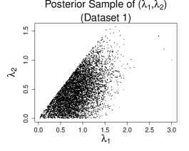
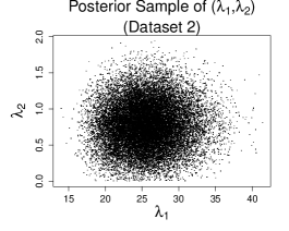
Figure 1: Sample from the joint posterior distribution of $\lambda_{1}$ and $\lambda_{2}$ for Dataset 1 (left) and Dataset 2 (right) as described in Section 4.

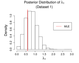
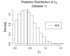
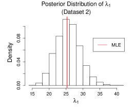
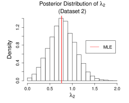
Figure 2: Marginal posterior densities and ACFs for $\lambda_{1}$ and $\lambda_{2}$ for Dataset 1 (top) and Dataset 2 (bottom) in Section 4.

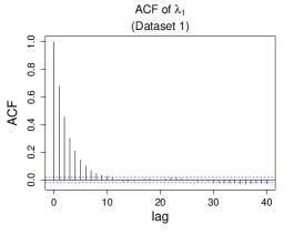
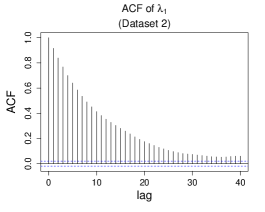
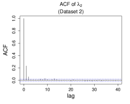
Figure 3: ACFs for $\lambda_{1}$ and $\lambda_{2}$ for Dataset 1 (top) and Dataset 2 (bottom) in Section 4.

4.2 Earthquake data

As an illustration of an application to real data, we consider an analysis of earthquake data recently analysed by Arnold and Jupp (2013). An earthquake gives rise to three orthogonal axes, and geophysicists are interested in analysing such data in order to compare earthquakes at different locations and/or at different times. An earthquake gives rise to a pair of orthogonal axes, known as the compressional (P) and tensional (T) axes, from which a third axis, known as the null (A) axis is obtained via $A=P\times T$. Each of these quantities are determined only up to sign, and so models for axial data are appropriate. The data can be treated as orthogonal axial $3$-frames in $\mathbb{R}^{3}$ and analysed accordingly, as in Arnold and Jupp (2013), but we will illustrate our method using the A axes only. In general, an orthogonal axial $r$-frame in $\mathbb{R}^{p},\hskip 2.84544ptr\leq p$, is an ordered set of $r$ axes, $\{\pm u_{1},\ldots,\pm u_{r}\}$, where $u_{1},\ldots,u_{r}$ are orthonormal vectors in $\mathbb{R}^{p}$ (Arnold and Jupp, 2013). The more familiar case of data on the sphere $\mathcal{S}^{2}$ is the special case corresponding to $p=3,r=1$, which is the case we consider here.

The data consist of three clusters of observations relating to earthquakes in New Zealand. The first two clusters each consist of $50$ observations near Christchurch which took place before and after a large earthquake on 22 February 2011, and we will label these two clusters CCA and CCB respectively. For these two clusters, the P and T axes are quite highly concentrated in the horizontal plane, and as a result the majority of the A axes are concentrated about the vertical axis. It is of interest to geophysicists to establish whether there is a difference between the pattern of earthquakes before and after the large earthquake. The third cluster is a more diverse set of $32$ observations obtained from earthquakes in the north of New Zealand’s South Island, and we will label this cluster SI. We will illustrate our method by fitting Bingham models to the A axes from each of the individual clusters and considering the posterior distributions of the Bingham parameters. We will denote the parameters from the CCA, CCB and SI models as $\lambda_{i}^{A}$, $\lambda_{i}^{B}$ and $\lambda_{i}^{S}$ respectively, $i=1,2$.

The observations for the two clusters of observations near Christchurch yield sample data of $(\tau_{1}^{A},\tau_{2}^{A})=(0.1152360,0.1571938)$ for CCA and $(\tau_{1}^{B},\tau_{2}^{B})(0.1127693,0.1987671)$ for CCB. The data for the South Island observations are $(\tau_{1}^{S},\tau_{2}^{S})=(0.2288201,0.3035098)$. We fit each dataset separately by implementing the proposed algorithm.Exponential prior distributions to all parameters of interest (mean 100) were assigned, subject to the constraint that $\lambda_{1}^{j}\geq\lambda_{2}^{j}$ for $j=A,B,S$. Scatter plots from the joint posterior distributions of the parameters from each individual analysis are shown in Figure 4. The plots for CCA and CCB look fairly similar, although $\lambda_{2}$ is a little lower for the CCB cluster. The plot for SI cluster suggests that these data are somewhat different.

Figure 4: Posterior samples for differences in $\lambda_{1}$ and $\lambda_{2}$ for the two sets of Christchurch data (left) and South Island and Christchurch data A (right). This shows a clear difference between the South Island and Christchurch data, but suggests no difference between the two sets of Christchurch data.

To establish more formally if there is any evidence of a difference between the two Christchurch clusters, we consider the bivariate quantity $(\lambda_{1}^{A}-\lambda_{1}^{B},\lambda_{2}^{A}-\lambda_{2}^{B}).$ If there is no difference between the two clusters, then this quantity should be $(0,0)$. In Figure 5 (left panel), we show the posterior sample of this quantity, and a 95% probability region obtained by fitting a bivariate normal distribution with parameters estimated from this sample. The origin is contained comfortably within this region, suggesting there is no real evidence for a difference between the two clusters. Arnold and Jupp (2013) obtained a $p$-value of $0.890$ from a test of equality for the two populations based on treating the data as full axial frames, and our analysis on the A axes alone agrees with this.

The right panel of Figure 5 shows a similar plot for the quantity $(\lambda_{1}^{A}-\lambda_{1}^{S},\lambda_{2}^{A}-\lambda_{2}^{S}).$ Here, the origin lies outside the 95% probability region, suggesting a difference between the first Christchurch cluster and the South Island cluster. Arnold and Jupp (2013) give a $p$-value of less than 0.001 for equality of the two populations, so again our analysis on the A axes agrees with this.

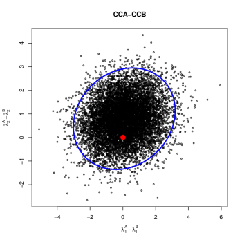
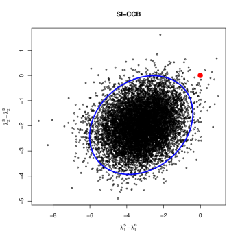
Figure 5: Posterior samples for differences in $\lambda_{1}$ and $\lambda_{2}$ for the two sets of Christchurch data (left) and South Island and Christchurch data A (right). This shows a clear difference between the South Island and Christchurch data, but suggests no difference between the two sets of Christchurch data.

5 Discussion

There is a growing area of applications that require inference over doubly intractable distributions including directional statistics, social networks (Caimo and Friel, 2011), latent Markov random fields (Everitt, 2012), and large–scale spatial statistics (Aune et al., 2012) to name but a few. Most conventional inferential methods for such problems relied on approximating the normalising constant and embedded the latter into a standard MCMC algorithm (e.g. Metropolis-Hastings). Such approaches not only are only approximate in the sense that the target distribution is an approximation to the true posterior distribution of interest, but they can also suffer from being very computationally intensive. It is only until fairly recently that algorithms which avoid the need of approximating/evaluating the normalising constant became available; see Møller et al. (2006); Murray et al. (2006); Walker (2011); Girolami et al. (2013).

In this paper we were concerned with exact Bayesian inference for the Bingham distribution which has been a difficult task so far. We proposed an MCMC algorithm which allows us to draw samples from the posterior distribution of interest without having to approximate this constant. We have shown that the MCMC scheme is i) fairly straightforward to implement, ii) mixes very well in a relatively short number of sweeps and iii) does not require the specification of good guesses of the unknown parameters. We have applied our method to both real and simulated data, and showed that the results agree with maximum likelihood estimates for the parameters. However, we believe that a fully Bayesian approach has the benefit of providing an honest assessment of the uncertainty of the parameter estimates and allows exploration of any non-linear correlations between the parameters of interest. In comparison to the approach recently proposed by Walker (2013) (which also avoids approximating the normalising constant) we argue that our algorithm is easier to implement, runs faster and the Markov chains appear to mix better.

In terms of the further computational aspects, our algorithm is not computationally intensive and this is particularly true for the number of dimensions that are commonly met in practice (e.g. $q=3$). For all the results presented here, we ran our MCMC chains for $10^{6}$ iterations for each of the simulated and real data examples, which we found to be sufficient for good mixing in all cases. Our method was implemented in C++ and each example took between $20$ and $30$ seconds on a desktop PC with 3.1GHz processor; note, that is considerably faster than the algorithm proposed by Walker (2013) in which “running $10^{5}$ iterations takes a matter of minutes on a standard laptop”. In general the time taken for our proposed algorithm will depend on the number of auxiliary data points $n$ that need to be simulated, as well as the efficiency of the underlying rejection algorithm for the particular parameter values at each iteration. In addition, the efficiency of the rejection algorithm is likely to deteriorate as the dimension $q$ increases, but we found it to be very efficient for all our examples and it is reasonably efficient for at least a moderate number of dimensions according to simulations by Ganeiber (2012).

Statistical inference, in general, is not limited to parameter estimation. Therefore, a possible direction for future research within this context is to develop methodology to enable calculation of the model evidence (marginal likelihood). This quantity is vital in Bayesian model choice and knowledge of it will allow a formal comparison between competing models for a given dataset such as the application presented in Section 4.2.

References

- (1)
- Arnold and Jupp (2013) Arnold, R. and Jupp, P. E. (2013). Statistics of orthogonal axial frames, Biometrika 100(3): 571–586.
- Aune et al. (2012) Aune, E., Simpson, D. P. and Eidsvik, J. (2012). Parameter estimation in high dimensional gaussian distributions, Statistics and Computing pp. 1–17.
- Bingham (1974) Bingham, C. (1974). An antipodally symmetric distribution on the sphere, Ann. Statist. 2: 1201–1225.
- Boomsma et al. (2008) Boomsma, W., Mardia, K., Taylor, C., Ferkinghoff-Borg, J., Krogh, A. and Hamelryck, T. (2008). A generative, probabilistic model of local protein structure., Proc Natl Acad Sci U S A 105(26): 8932–7.
- Caimo and Friel (2011) Caimo, A. and Friel, N. (2011). Bayesian inference for exponential random graph models, Social Networks 33(1): 41–55.
- Ehler and Galanis (2011) Ehler, M. and Galanis, J. (2011). Frame theory in directional statistics, Statistics and Probability Letters 81(8): 1046–1051.
- Everitt (2012) Everitt, R. G. (2012). Bayesian parameter estimation for latent markov random fields and social networks, Journal of Computational and Graphical Statistics 21(4): 940–960.
- Ganeiber (2012) Ganeiber, A. M. (2012). Estimation and simulation in directional and statistical shape models, PhD thesis, University of Leeds.
- Girolami et al. (2013) Girolami, M., Lyne, A.-M., Strathmann, H., Simpson, D. and Atchade, Y. (2013). Playing russian roulette with intractable likelihoods, ArXiv preprint; arXiv:1306.4032 .
-
Kent (1987)
Kent, J. T. (1987).
Asymptotic expansions for the Bingham distribution, J. Roy.
Statist. Soc. Ser. C 36(2): 139–144.
http://dx.doi.org/10.2307/2347545 - Kent and Ganeiber (2012) Kent, J. T. and Ganeiber, A. M. (2012). Simulation of the Bingham distribution in directional statistics, in K. V. Mardia, A. Gusnato, A. D. Riley and J. Voss (eds), New Statistics and Modern Natural Sciences, Leeds University Press, Leeds, pp. 57–59.
-
Kume and Walker (2006)
Kume, A. and Walker, S. G. (2006).
Sampling from compositional and directional distributions, Stat.
Comput. 16(3): 261–265.
http://dx.doi.org/10.1007/s11222-006-8077-9 -
Kume and Wood (2005)
Kume, A. and Wood, A. T. A. (2005).
Saddlepoint approximations for the Bingham and Fisher-Bingham
normalising constants, Biometrika 92(2): 465–476.
http://dx.doi.org/10.1093/biomet/92.2.465 -
Kume and Wood (2007)
Kume, A. and Wood, A. T. A. (2007).
On the derivatives of the normalising constant of the Bingham
distribution, Statist. Probab. Lett. 77(8): 832–837.
http://dx.doi.org/10.1016/j.spl.2006.12.003 - Levine et al. (2002) Levine, J. D., Funes, P., Dowse, H. B. and Hall, J. C. (2002). Resetting the circadian clock by social experience in drosophila melanogaster, Science Signaling 298(5600): 2010–2012.
- Mardia and Jupp (2000) Mardia, K. V. and Jupp, P. E. (2000). Directional statistics, Wiley Series in Probability and Statistics, John Wiley & Sons Ltd., Chichester. Revised reprint of ıt Statistics of directional data by Mardia [ MR0336854 (49 #1627)].
- Mardia and Zemroch (1977) Mardia, K. V. and Zemroch, P. J. (1977). Table of maximum likelihood estimates for the bingham distribution, Statist. Comput. Simul. 6: 29–34.
-