Dust reverberation mapping in the era of big optical surveys
and its cosmological application

Abstract

The time lag between optical and near-infrared (IR) flux variability can be taken as a means to determine the sublimation radius of the dusty “torus” around supermassive black holes in active galactic nuclei (AGN). I will show that data from big optical survey telescopes, e.g. the Large Synoptic Survey Telescope (LSST), can be used to measure dust sublimation radii as well. The method makes use of the fact that the Wien tail of the hot dust emission reaches into the optical and can be reliably recovered with high-quality photometry. Simulations show that dust sublimation radii for a large sample of AGN can be reliably established out to redshift $z\sim 0.1-0.2$ with the LSST. Owing to the ubiquitous presence of AGN up to high redshifts, they have been studies as cosmological probes. Here, I discuss how optically-determined dust time lags fit into the suggestion of using the dust sublimation radius as a “standard candle” and propose and extension of the dust time lags as “standard rulers” in combination with IR interferometry.

1. Introduction

The near-infrared (IR) light curves of active galactic nuclei (AGN) show variability that is consistent with the optical light curves, however lagging by tens to hundreds of days (e.g. Clavel et al., 1989; Glass, 1992; Oknyanskij et al., 1999; Glass, 2004; Suganuma et al., 2006; Koshida et al., 2009). The lag supposedly represents the distance from the central engine to the region where the temperature drops to about 1500 K so that dust can marginally survive. This sublimation radius, $R_{\mathrm{sub}}$, has been found to scale with the square-root of the AGN luminosity using both time delay (e.g. Oknyanskij & Horne, 2001; Minezaki et al., 2004; Suganuma et al., 2006; Kishimoto et al., 2011a) and IR interferometric measurements(e.g. Kishimoto et al., 2011a), as expected from dust in local thermal equilibrium (e.g. Barvainis, 1987).

Both IR interferometry and dust reverberation mapping are limited by their technical requirements of either sensitive long-baseline arrays or simultaneous availability of optical and IR instrumentation. Here, I will show that upcoming large optical surveys can recover time lags from hot dust emission for a huge number of AGN using optical bands, therefore overcoming some of these limitations.

Since AGN are ubiquitous in the universe, they may be attractive targets as cosmological probes. Both the broad-line region (BLR) radius (Haas et al., 2011; Watson et al., 2011; Czerny et al., 2013) and hot-dust radius (e.g. Kobayashi et al., 1998; Oknyanskij, 1999, 2002; Yoshii et al., 2004) seem promising “standard candles”, based on the observationally well-established BLR lag-luminosity (e.g. Kaspi et al., 2000; Peterson et al., 2004) and NIR lag-luminosity relations (e.g. Oknyanskij & Horne, 2001; Minezaki et al., 2004; Suganuma et al., 2006). For the BLR, Elvis & Karovska (2002) proposed that a combination of interferometric observations of emission lines and lag times may be used as “standard rulers”, thus bypassing the cosmic distance ladder. Here, I suggest that the hot-dust lags and near-IR interferometric sizes can also serve as standard rulers, although requiring advancements in IR interferometry.

2. Principles of dust reverberation mapping at optical wavelengths

Dust around AGN absorbs the UV/optical radiation from the putative accretion disk and reemits in the IR. At about 1500 K, the dust sublimates, corresponding to the hottest dust emission peaking at $\sim 2\,\micron$. Despite the exponential decrease of the Wien tail, some contribution of the hot-dust emission will reach into optical wavebands. Indeed, such a dust contribution has been reported by Sakata et al. (2010) in the $I$-band from analyzing the color variability of optical variability. Therefore, the optical emission consists of contributions from two different emission regions, leading to a relative lag.

Dust is considered to be in local thermal equilibrium (LTE), allowing us to calculate the dust temperature/emission directly from the absorbed incident radiation. In Hönig & Kishimoto (2011), we presented a theoretical framework showing that these LTE considerations can be used to calculate temperature changes $\mathrm{d}T$ for variable incident radiation $\mathrm{d}L$ as $\mathrm{d}T/T=1/4\,\mathrm{d}L/L$ . Based on this relation, changes in the temperature and emission of a pre-defined dust distribution can be calculated to derive near-IR light curves (Hönig & Kishimoto, 2011).

The optical emission is dominated by the AGN central engine’s “big blue bump” (BBB). The BBB spectral energy can be approximated as $\lambda F_{\lambda}\propto\lambda^{-4/3}$ (e.g. Elvis et al., 1994; Richards et al., 2006; Stern & Laor, 2012). For the purpose of this study, I will assume that the host galaxy is constant and readily removable by image decomposition and that broad- and narrow-lines do not contribute significantly ($\lesssim 1-10\%$) to the broad-band fluxes (see Sect. 4.1). Therefore, the AGN emission in the optical can be approximated by

$$F_{\mathrm{AGN}} =F_{V}\cdot\left(\frac{\lambda}{0.55\,\micron}\right)^{-7/3}$$ (1)

$$+\frac{F_{\mathrm{BBB}}(1.2\,\micron)}{\pi B_{\mathrm{1.2\,\micron}}(1400\,K)}\cdot\pi B_{\mathrm{\lambda}}(1400\,K)$$

$F_{V}$ denotes the $V$-band flux at $0.55\,\micron$, $F_{\mathrm{BBB}}(1.2\,\micron)$ is the BBB flux component at 1.2 $\micron$, and $\pi B_{\mathrm{1.2\,\micron}}(1400\,K)$ represents the flux of a 1400 K black body at 1.2 $\micron$ (observed near-IR color temperature; Kishimoto et al., 2007, 2011b). The normalization accounts for the fact that AGN show a generic turnover from BBB-dominated emission to host-dust emission at about $1-1.2\,\micron$ (e.g. Neugebauer et al., 1979; Elvis et al., 1994).

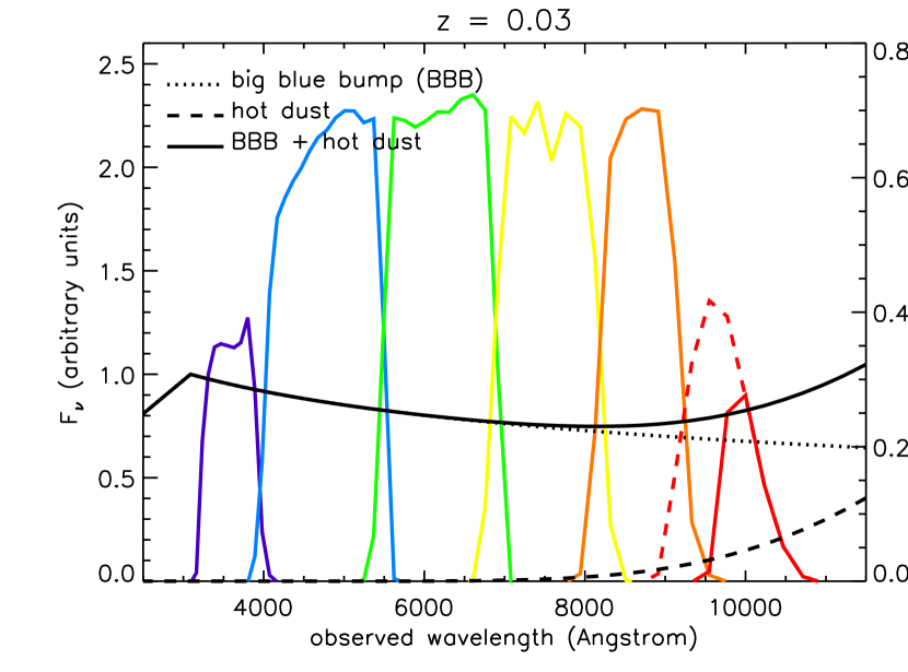
Figure 1.— AGN template SED for a redshift of $z=0.03$ in the wavelength range from $2500-20\,000\AA$. The dotted line is the big-blue bump component and the dashed line represents a black-body with temperature $T=1500\,$K. The solid line is the combination of both emission components. The colored solid lines illustrate the transmission of the LSST $u$, $g$, $r$, $i$, $z$, and $y3$ wavebands (violet to red), respectively. The dashed-red line shows the alternative $y4$ filter.

Table 1Relative contributions of hot dust to wavebands at different redshifts.

redshift	$z=0$	$z=0.05$	$z=0.1$	$z=0.2$	$z=0.3$
$i$ band	0.019	0.012	0.007	0.003	$\ldots$
$z$ band	0.073	0.052	0.031	0.014	0.004
$y$ band ($y3$)	0.206	0.158	0.109	0.053	0.020
$y$ band ($y4$)	0.168	0.126	0.085	0.041	0.015

Fig. 1 shows the total AGN SED, the BBB, and hot-dust components for a simulated object at redshift $z=0.03$. Overplotted are the transmission curves for the LSST filters $u$, $g$, $r$, $i$, $z$, and $y$, where the latter may either be represented by the $y3$ (referred to as $y$ in the following) or $y4$ filter. The Wien tail of the hot dust reaches into the $z$ and $y$ bands. However, the fractional contribution of the dust is very sensitive to the object’s redshift. In Table 1, hot-dust contributions to the total flux in $i$, $z$, and $y$ are listed for $0<z<0.3$. Out to about $z\sim 0.1$ the dust contribution to the $y$ band is $\gtrsim$10% and drops to $\sim$5% at $z=0.2$. Therefore, the dust component may be detected above the BBB out to $z\sim 0.1-0.2$.

3. A dust reverberation mapping experiment for optical surveys

In this letter I propose to use optical wavebands for dust reverberation mapping of AGN. Suitable telescope projects are currently being explored or under construction. The most promising survey for this experiment will be the LSST. Its cornerstones are high photometric quality ($<$1%), high cadence, and multi-year operation. The feasibility for LSST will be illustrated in the following. It can be easily translated to other surveys.

3.1. Simulation of observed light curves and construction of a mock survey

First, it is necessary to simulate survey data and find a method that allows for recovering dust time lags. Kelly et al. (2009) show that the optical variability is well reproduced by a stochastic model based on a continuous autoregressive process (Ornstein-Uhlenbeck process; see also Kelly et al., 2013). The model consists of a white noise process with characteristic amplitude $\sigma$ that drives exponentially-decaying variability with time scale $\tau$ around a mean magnitude $m_{0}$. The parameters $\sigma$ and $\tau$ have been found to scale with black hole mass $M_{\mathrm{BH}}$ and/or luminosity $L$ of the AGN (e.g. Kelly et al., 2009, 2013). For the simulations, $L$ and $M_{\mathrm{BH}}$ are chosen and $\sigma$ and $\tau$ are drawn from the error distribution of the respective relation given in Kelly et al. (2009). Since the amplitude of variability depends on wavelength, it was adjusted by $\sigma(\lambda)=\sigma\times(\lambda/5500\,\mathrm{\AA})^{-0.28}$ as empirically found by Meusinger et al. (2011).

The BBB light curves are then propagated outward into the dusty region. Its inner edge, $R_{\mathrm{sub}}$, and thus the dust time lag $\tau(R_{\mathrm{sub}})$, scales with $L$ as $R_{\mathrm{sub}}\propto\tau(R_{\mathrm{sub}})\propto L^{1/2}$. The reaction of the dust on BBB variability is modeled using the principles outlined in Sect. 2. For that, the dust is distributed in a disk with a surface density distribution $\Sigma(r)\propto r^{a}$, and the temperature of the dust at distance $r$ from the AGN is calculated using the black-body approximation for LTE, $T(r)=T_{\mathrm{sub}}\times(r/R_{\mathrm{sub}})^{-0.5}$ (sublimation temperature $T_{\mathrm{sub}}=1500\,$K). The power law index $a$ represents the compactness of the dust distribution ($a$ very negative = compact; $a\sim 0$ = extended) and results in smearing out the variability signal/transfer function. Since its actual value is rather unconstrained, a random value is picked in the range $-2.5<a<-0.5$, motivated by observations (Hönig et al., 2010; Kishimoto et al., 2011b; Hönig et al., 2012, 2013). Using the dust variability model on actual data showed that only a fraction of the incident variable BBB energy, $w_{\mathrm{eff}}$, is converted into hot-dust variability (for details see Hönig & Kishimoto, 2011). Thus, a random $w_{\mathrm{eff}}$ is picked in the interval $w_{\mathrm{eff}}\ \epsilon\ [0.2,0.8]$ for each simulated AGN. In summary, the hot dust emission and its variability is fully characterized by $a$ and $w_{\mathrm{eff}}$.

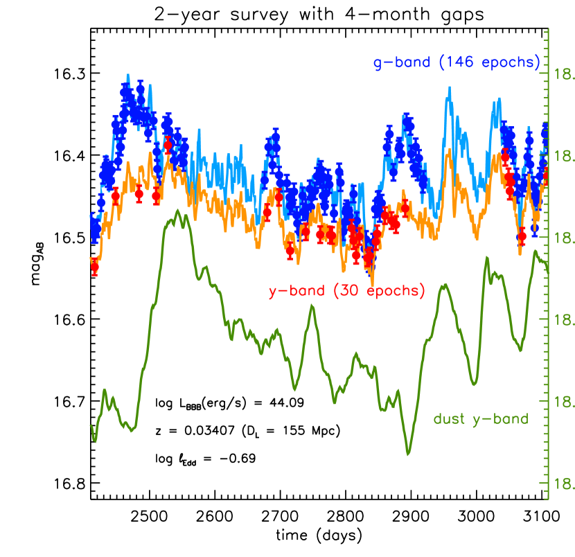
Figure 2.— Simulated AGN light curves in the $g$- (light blue) and $y$-band (light red) filters for a period of two years. The blue and red circles with error bars represent mock observations of these $g$- and $y$-band light curves, respectively, based on the LSST photometric precision and an average sampling of 4 days ($g$-band) and 17 days ($y$-band). The green line represents the dust-only model light curve in the $y$-band (magnitude scale on right axis). The AGN characteristics are listed in the top-left corner.

Magnitudes at all LSST wavebands are extracted for the combined BBB + hot-dust emission for AGN with luminosities $L$ at distances $D_{L}$. The “mock observations” take into account the expected statistical and systematic errors of the LSST . It is assumed that each AGN is observed once every 7 days in $u$, 3 days in $g$, 5 days in $r$, 10 days in $i$, 20 days in $z$, and 15 days in $y$.

For illustration of the proposed method, AGN properties observed in the local universe ($z\lesssim 0.1$) were approximated as follows: First, a redshift is randomly picked from a $(1+z)^{3}$-distribution. Then, luminosities are drawn randomly from the interval $\log L(\mathrm{erg/s})\epsilon[42.7,44.3]$ and adjusted by $10\cdot z$ (quasars become more abundant with $z$). $M_{\mathrm{BH}}$ is determined based on $L$ and an Eddington ratio picked randomly around the $L$-dependent mean $\log\left<\ell_{\mathrm{Edd}}\right>=-1.0+0.3\times\log L/\left<L\right>$ (Gaussian with standard deviation $\sigma_{\log\ell}=0.22\,$dex), producing an $L$-$\ell_{\mathrm{Edd}}$ correlation.

3.2. How to recover dust time lags

A catalog with 301 AGN has been simulated. Example light curves in the $g$ and $y$ bands are presented in Fig. 2. The circles with error bars are the observed epochs that will be used as input for the reverberation experiment. In the following, a very simple cross-correlation approach will be used to successfully recover dust lags. The intention is to provide a proof-of-concept, while optimization or tests of better approaches (e.g. Chelouche & Daniel, 2012; Chelouche & Zucker, 2013; Zu et al., 2013) are encouraged for future studies.

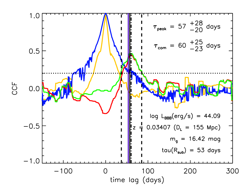
Figure 3.— Six-days-smoothened cross-correlation function (CCF) of an AGN (catalog ID 160). The red line shows the CCF between the $y-$BBB light curve and the BBB light curve, while the blue and orange lines are auto-correlation functions of the BBB and $y-$BBB light curves, respectively. The green line is the $y-BBB$ CCF after subtracting a scaled combination of the two ACFs. The dotted line marks the CCF cutoff for automated time-delay detection. The black-solid and -dashed-dotted lines denote the auto-detected peak time lag $\tau_{\mathrm{peak}}$ and center-of-mass time lag $\tau_{\mathrm{com}}$, respectively. The dashed lines mark the error regions where the CCF is half of its peak value. For reference, the purple-solid line marks the time lag of the sublimation radius in the input model. The AGN input properties are listed as well.

First, the observed photometric light curves in each band and with very different time resolution and inhomogeneous coverage were resampled to a common $\Delta t=1$ day using the stochastic interpolation technique described in (Peterson et al., 1998) and Suganuma et al. (2006). For each band, 10 random realizations of the resampled light curves were simulated. From the resampled $ugri$ light curves, a reference BBB light curve was extracted. For that, the mean fluxes and standard deviations over the 10 random realizations of each band and epoch were calculated and a simple power law $f_{\mathrm{\nu}}\propto\nu^{\beta}$ was fit to the resulting $ugri$ fluxes at each resampled epoch. Based on this fit, a $V$-band flux at 0.55 $\micron$ was determined. This method uses the maximum information of all bands simultaneously and the resulting BBB light curve is very close to the input AGN variability pattern.

In the next step, the BBB light curve was subtracted from the $y$ band fluxes. This procedure can produce negative fluxes and leaves some BBB variability in the result because of the overestimation of the BBB underlying the $y$ band and the wavelength-dependence of the variability. However, as we are interested only in the time delay signal, this does not need to be of concern. The most important result from this procedure is that a large part of the BBB signal has been removed in this $y-$BBB light curve.

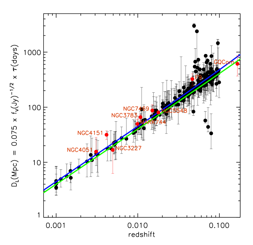
Figure 4.— Redshift-independent luminosity distances based on dust time lags and AGN $V$-band flux plotted against redshift. The black circles with error bars are AGN from the mock survey. The red points are observed AGN with known dust time lags. The blue line shows the $z-D_{\mathrm{L}}$ relation for the Planck cosmological parameters, while the green line assumes $H_{0}=75$ (km/s)/Mpc, $\Omega_{m}=1$ and $\Omega_{\Lambda}=0$.

Finally, the observed epochs of the $y-$BBB light curve are (discretely) cross-correlated with the BBB light curve by interpolating the BBB flux at the observed $y$ band epochs and accounting for different lags. An example cross-correlation function (CCF) for a ten-year LSST survey, smoothed with a box-car kernel with a width of 6 days, is shown in Fig. 3. The CCF shows a distinct negative/anti-correlation peak at zero lag. This peak originates from the subtraction method discussed above. As such, it closely follows the auto-correlation functions of the BBB and $y-$BBB light curves. After linearily-combining both ACFs and scaling to the 0-lag negative peak, the BBB effect on the CCF can be effectively removed.

To recover the dust lag, the highest peak in the CCF after ACF subtraction was automatically identified. A positive detection is considered if the peak CCF $\geq$0.2. An error region is defined as the range over which the CCF is at least half the peak CCF. The maximum CCF defines the time lag of the peak $\tau_{\mathrm{peak}}$. A center-of-mass time lag $\tau_{\mathrm{com}}$ is also determined at half the integrated CCF within the error region.

As a final remark, a direct cross-correlation between the observed $y$ band and any optical band did not recover a time delay, although a corresponding peak is seen when cross-correlating the input model light curves. In addition, the “shifted reference” method by Chelouche & Daniel (2012) developed to recover time lags of the BLR from photometric filters was not successful. This originates from the fact that the target signal does not vary with the same amplitude as the reference band and is significantly smeared, and may require the refinement presented in Chelouche & Zucker (2013).

4. Discussion

4.1. Time delays in a real survey

The quality of lag recovery critically depends on the cadence as well as the continuity of observations. Typically, objects will not be observable year-round. In order to simulate this effect, annual gaps of 2, 4, and 6 months were introduced for 1/6, 1/3, and 1/2 of the catalog, respectively. Due to strong noise features for lags longer than $\sim$350 days, the CCF was analyzed only for lags $<$300 days. In general, lags are detected for about 70% or more of all AGN, independent of gap length. Out of these lags, about 80% are consistent within error bars with the sublimation radius of the input model. This is arguably a high rate given the simplicity of the lag recovery scheme and the completely blind analysis without any human interaction. The success rates might be boosted with more sophisticated methods and a way to deal with the longer lags. Note that these numbers are strictly valid only for the specific AGN sample parameters (see Sect. 3.1).

There are some issues that merit further attention. The current simulations do not take into account contributions of broad lines. This should be a minor issue for the recovery of the BBB light curve given the multi-filter fitting scheme. However, broad components of Paschen lines in the $y$-band may impose a secondary lag signal onto the dust light curve (see Chelouche & Daniel, 2012, for Balmer lines). While their contribution is probably smaller than the dust contribution in this band (see spectra in Landt et al., 2011), they should be part of a more advanced recovery scheme (see Sect 3.2). Furthermore, potential scattered light from the BBB (e.g. Kishimoto et al., 2008; Gaskell et al., 2012) and the Paschen continuum are also neglected, but their contribution to the total $y$-band flux is estimated to be of the order of 1%.

The host flux has been neglected in the modeling (see Sect. 2). Based on the optical AGN/host decomposition of Bentz et al. (2009), the contribution of the host to the total flux can reach 50% at $L_{\mathrm{AGN}}\lesssim 10^{43}$ erg/s and will drop to $\sim$10% for $L_{\mathrm{AGN}}\lesssim 10^{45}$ erg/s in the $V$-band. Therefore, if the host contribution was considered, the presented simulations would apply to a sample that is brighter by $\sim 0.1-0.7$  mag.

4.2. Cosmological applications of dust time lags and dust emission sizes

Radius-luminosity relations open up the possibility to use AGN as “standard candles” in cosmology. Such applications have been discussed for both the BLR (Haas et al., 2011; Watson et al., 2011) and the dust (e.g. Kobayashi et al., 1998; Oknyanskij, 1999, 2002; Yoshii et al., 2004). While the current AGN reverberation sample is larger for the BLR than for the hot dust, the proposed use of optical surveys may change this picture significantly. Fig. 4 shows the 231 objects from the 301-object mock AGN catalog for which time lags $\tau_{\mathrm{peak}}$ were recovered. For each of these AGN, the $V$-band flux $f_{V}$ was measured and a luminosity distance $D_{L}$ independent of redshift was calculated as

$$D_{L}(\mathrm{Mpc})=0.075\times f_{V}(\mathrm{Jy})^{-1/2}\times\tau_{\mathrm{peak}}(\mathrm{days})\ .$$ (2)

The scaling factor of 0.075 was obtained by fitting $f_{V}^{-1/2}\cdot\tau$ to the known distances of the objects in the mock survey (a real survey will require normalizing to the cosmic distance ladder). The errors of individual data points are dominated by the uncertainties in $\tau$ as long as $f_{V}$ can be determined with $\lesssim 30\%$ accuracy. Overplotted are $z-D_{L}$-relations for a standard cosmology according to the latest Planck results ($H_{0}=67.3$ (km/s)/Mpc, $\Omega_{m}=0.315$, $\Omega_{\Lambda}=0.685$) as well as for a universe without cosmological constant ($H_{0}=75$ (km/s)/Mpc, $\Omega_{m}=1$, $\Omega_{\Lambda}=0$). For comparison, $K$-band reverberation-mapped AGN from literature are also shown (NGC 3227, NGC 4051, NGC 5548, NGC 7469: Suganuma et al. (2006); NGC 4151: Koshida et al. (2009); Fairall 9: Clavel et al. (1989); GQ Com: Sitko et al. (1993); NGC 3783: Glass (1992); Mark 744: Nelson et al. (1996)). The limitation to optical bands does not allow for distinguishing between different cosmological parameters. However, such a nearby sample ($z\lesssim 0.1$) can be used to determine the scaling factor. Under the same configuration as taken for the optical bands, a survey using near-IR filters will reach $z\sim 0.3$ in the $J$-band, $z\sim 0.7$ in the $H$-band, and $z\sim 1.3$ in the $K$-band.

One of the disadvantages of standard candles are their reliance on the cosmic distance ladder. This dependence can be overcome with “standard rulers” for which an angular diameter distance $D_{A}$ is determined by comparing physical with angular sizes. Elvis & Karovska (2002) proposed the use of AGN BLR time lags in combination with spatially- and spectrally-resolved interferometry of broad emission lines for this purpose. However, optical/near-IR interferometry of AGN needs 8-m class telescopes (e.g. at the VLTI or Keck) and is limited to about 130m baseline lengths. A broad emission line in the near-IR has only been successfully observed and resolved for one AGN to-date (3C273; Petrov et al., 2012).

Here, it is proposed that the dust time lags may also be used as a “standard ruler” in combination with directly measured near-IR angular sizes, $\rho_{K}$, from interferometry to determine angular size distances $D_{A}$, via the relation

$$D_{A}(\mathrm{Mpc})=0.126\times\frac{\tau(\mathrm{days})}{\xi_{\mathrm{int}}\cdot\rho_{K}(\mathrm{mas})}\ .$$ (3)

$\xi_{\mathrm{int}}$ corrects the different sensitivities of the CCF and interferometry measurements to extended dust distributions (e.g. Kishimoto et al., 2011a, 2014) and may be determined from spectral or interferometric modeling.

For both the standard candle and ruler, time lags for the hot dust have to be determined. As compared to the BLR, the dust lags are about a factor of 4 longer (comparing the $\mathrm{H\beta}$ relation in Bentz et al. (2009) with the dust relation in Kishimoto et al. (2007)), resulting in longer monitoring campaigns. On the other hand, dust monitoring does not require spectroscopy or the use of specific narrow-band filters, but can be executed with any telescope that has broad-band filters and sufficient sensitivity. Moreover, the hot-dust emission and sublimation radius are extremely uniform across AGN, e.g. showing a narrow range of color temperatures (e.g. Glass, 2004), a universal turn-over at $\sim 1-1.2\,\micron$ (e.g. Neugebauer et al., 1979; Elvis et al., 1994), and an emissivity close to order unity (e.g. Kishimoto et al., 2011b). This points toward simple physics (radiative reprocessing within $\sim\micron$-sized dust grains) involved in dust emission at $R_{\mathrm{sub}}$, which arguably removes some physical uncertainties that are inherent to other methods.

For hot dust radii as standard rulers, the emission region has to be spatially resolved without the need for spectral resolution. This has been achieved for 13 nearby AGN to-date ($z\leq 0.16$; e.g. Kishimoto et al., 2011a; Weigelt et al., 2012; Kishimoto et al., 2014) with the limiting factor being sensitivity of IR interferometers. However, using a potential km-sized heterodyne array (e.g. the Planet Formation Imager with sufficient wavelength coverage into the $L$ and $M$ bands, space-based or on the ground, may allow for direct distance estimates directly into the Hubble flow out to $z\gtrsim 1$, entirely bypassing the cosmological distance ladder (Hönig et al., in prep.).

References

- Barvainis (1987) Barvainis, R. 1987, ApJ, 320, 537
- Bentz et al. (2009) Bentz, M. C., Peterson, B., M., Netzer, H., Pogge, R. W., & Vestergaard, M. 2009, ApJ, 697, 160
- Chelouche & Daniel (2012) Chelouche, D., & Daniel, E. 2012, ApJ, 747, 62
- Chelouche & Zucker (2013) Chelouche, D., & Zucker, S. 2013, ApJ, 769, 124
- Clavel et al. (1989) Clavel, J., Wamsteker, W., & Glass, I. S. 1989, ApJ, 337, 236
- Czerny et al. (2013) Czerny, B., Hryniewicz, K., Maity, I., et al. 2013, A&A, 556, A97
- Elvis et al. (1994) Elvis, M., Wilkes, B. J., McDowell, J. C., Green, R. F., et al. 1994, ApJSS, 95, 1
- Elvis & Karovska (2002) Elvis, M., & Karovska, M. 2001, ApJL, 581, 67
- Gaskell et al. (2012) Gaskell, C. M., Goosmann, R. W., Merkulova, N. I., Shakhovskoy, N. M., & Shoji, M. 2012, ApJ. 749, 148
- Glass (1992) Glass, I. S. 1992, MNRAS, 256, 23
- Glass (2004) Glass, I. S. 2004, MNRAS, 350, 1049
- Haas et al. (2011) Haas, M., Chini, R., Ramolla, M., et al. 2011, A&A, 535, A73
- Hönig et al. (2010) Hönig, S. F., Kishimoto, M., Gandhi, P., et al. 2010, A&A, 515, 23
- Hönig & Kishimoto (2010) Hönig, S. F., & Kishimoto, M. 2010, A&A, 523, 27
- Hönig & Kishimoto (2011) Hönig, S. F., & Kishimoto, M. 2011, A&A, 534, 121
- Hönig et al. (2012) Hönig, S. F., Kishimoto, M., Antonucci, R., et al. 2012, ApJ, 755, 149
- Hönig et al. (2013) Hönig, S. F., Kishimoto, M., Tristram, K. R. W., et al. 2013, ApJ, 771, 87
- Kaspi et al. (2000) Kaspi, S., Smith, P. S., Netzer, H., et al. 2000, ApJ, 553, 631
- Kelly et al. (2009) Kelly, B., C., Bechthold, J., & Siemiginowska, A. 2009, ApJ, 698, 895
- Kelly et al. (2013) Kelly, B., C., Treu, T., Malkan, M., et al. 2013, ApJ, submitted (arXiv:1307.5253)
- Kishimoto et al. (2007) Kishimoto, M., Hönig, S. F., Beckert, T., & Weigelt, G. 2007, A&A, 476, 713
- Kishimoto et al. (2008) Kishimoto, M., Antonucci, R., Blaes, O., et al. 2008, Nature, 454, 492
- Kishimoto et al. (2011a) Kishimoto, M., Hönig, S. F., Antonucci, R., et al. 2011a, A&A, 527, 121
- Kishimoto et al. (2011b) Kishimoto, M., Hönig, S. F., Antonucci, R., et al. 2011b, A&A, 536, 78
- Kishimoto et al. (2013) Kishimoto, M., Hönig, S. F., Antonucci, R., et al. 2013, ApJ, 775, L36
- Kishimoto et al. (2014) Kishimoto, M., et al. 2014, A&A, submitted
- Kobayashi et al. (1998) Kobayashi, Y., Yoshii, Y., Peterson, B. A., et al. 1998, SPIE, 3354, 769
- Koshida et al. (2009) Koshida, S., Yoshii, Y., Kobayashi, Y., et al. 2009, ApJ, 700, L109
- Landt et al. (2011) Landt, H., Elvis, M., Ward, M. J., et al. 2011, MNRAS, 414, 218
- Meusinger et al. (2011) Meusinger, H., Hinze, A., & de Hoon, A. 2011, A&A, 525, 37
- Neugebauer et al. (1979) Neugebauer, G., Oke, J. B., Becklin, E. E., & Matthews, K. 1979, ApJ, 230, 79
- Minezaki et al. (2004) Minzaki, T., Yoshii, Y., Kobayashi, Y., et al. 2004, ApJL, 600, 35
- Mor & Netzer (2011) Mor, R., & Netzer, H. 2011, ApJ, 420, 526
- Nelson et al. (1996) Nelson, B. O. 1996, ApJ, 465, L87
- Oknyanskij et al. (1999) Oknyanskij, V. L., Lyuty, V. M., Taranova, O. G., & Shenavrin, V. I. 1999, AstL, 25, 483
- Oknyanskij (1999) Oknyanskij, V. L. 1999, OAP, 12, 99
- Oknyanskij & Horne (2001) Oknyanskij, V. L., & Horne, K. 2001, ASPC, 224, 149
- Oknyanskij (2002) Oknyanskij, V. L. 2002, ASPC, 282, 330
- Peterson et al. (1998) Peterson, B. M., Wanders, I., Horne, K., et al. 1998, PASP, 110, 660
- Peterson et al. (2004) Peterson, B. M., Ferrarese, L., Gilbert, K. M., et al. 2004, ApJ, 613, 682
- Petrov et al. (2012) Petrov, R. G., Millour, F., Lagarde, S., et al. 2012, SPIE, 8445, 88450W
- Richards et al. (2006) Richards, G. T., Lacy, M., Storrie-Lombardi, L. J., Hall, P. B., et al. 2006, ApJSS, 166, 470
- Sakata et al. (2010) Sakata, Y., Minezaki, T., Yoshii, Y., et al. 2010, ApJ, 711, 461
- Sitko et al. (1993) Sitko, M. L., Sitko, A. K., Siemiginowska, A., & Szczerba, R., 1993, ApJ, 409, 139
- Stern & Laor (2012) Stern, J., & Laor, A. 2012, MNRAS, 423, 600
- Suganuma et al. (2006) Suganuma, M., Yoshii, Y., Kobayashi, Y., et al. 2006, ApJ, 639, 46
- Watson et al. (2011) Watson, D., Denney, K. D., Verstergaard, M., & Davis, T. M. 2011, ApJL, 740, 49
- Weigelt et al. (2012) Weigelt, G., Hofmann, K.-H., Kishimoto, M., et al. 2012, A&A, 541, L9
- Yoshii et al. (2004) Yoshii, Y., Kobayashi, Y., & Minezaki, T. 2004, AN, 325, 540
- Zu et al. (2013) Zu, Y., Kochanek, C. S., Kozlowski, S., & Peterson, B. M. 2013, arXiv:1310.6774