The clustering of galaxies in the SDSS-III Baryon Oscillation Spectroscopic Survey: modeling of the luminosity and colour dependence in the Data Release 10

Abstract

We investigate the luminosity and colour dependence of clustering of CMASS galaxies in the Sloan Digital Sky Survey-III Baryon Oscillation Spectroscopic Survey Tenth Data Release, focusing on projected correlation functions of well-defined samples extracted from the full catalog of $\sim 540,000$ galaxies at $z\sim 0.5$ covering about $6,500\,\deg^{2}$. The halo occupation distribution framework is adopted to model the measurements on small and intermediate scales (from $0.02$ to $60\,h^{-1}{\rm{Mpc}}$), infer the connection of galaxies to dark matter halos and interpret the observed trends. We find that luminous red galaxies in CMASS reside in massive halos of mass $M{\sim}10^{13}$–$10^{14}\,h^{-1}{\rm M_{\sun}}$ and more luminous galaxies are more clustered and hosted by more massive halos. The strong small-scale clustering requires a fraction of these galaxies to be satellites in massive halos, with the fraction at the level of 5–8 per cent and decreasing with luminosity. The characteristic mass of a halo hosting on average one satellite galaxy above a luminosity threshold is about a factor $8.7$ larger than that of a halo hosting a central galaxy above the same threshold. At a fixed luminosity, progressively redder galaxies are more strongly clustered on small scales, which can be explained by having a larger fraction of these galaxies in the form of satellites in massive halos. Our clustering measurements on scales below $0.4\,h^{-1}{\rm{Mpc}}$ allow us to study the small-scale spatial distribution of satellites inside halos. While the clustering of luminosity-threshold samples can be well described by a Navarro-Frenk-White (NFW) profile, that of the reddest galaxies prefers a steeper or more concentrated profile. Finally, we also use galaxy samples of constant number density at different redshifts to study the evolution of luminous red galaxies, and find the clustering to be consistent with passive evolution in the redshift range of $0.5\lesssim z\lesssim 0.6$.

1 Introduction

Galaxy luminosity and colour, the two readily measurable quantities, encode important information about galaxy formation and evolution processes. The clustering of galaxies as a function of luminosity and colour helps reveal the role of environment in such processes. The dependence of clustering on such galaxy properties is therefore a fundamental constraint on theories of galaxy formation, and it is also important when attempting to constrain cosmological parameters with galaxy redshift surveys, since the different types of galaxies trace the underlying dark matter distribution differently. In this paper, we present the modeling of the luminosity and colour dependent clustering of massive galaxies in the Sloan Digital Sky Survey-III (SDSS-III; Eisenstein et al., 2011).

A fundamental measure of clustering is provided by measuring galaxy two-point correlation functions (2PCFs). Galaxy clustering provides a powerful approach to characterize the distribution of galaxies and probe the complex relation between galaxies and dark matter. More luminous and redder galaxies are generally observed, in various galaxy surveys, to have higher clustering amplitudes than their fainter and bluer counterparts (e.g. Davis & Geller, 1976; Davis et al., 1988; Hamilton, 1988; Loveday et al., 1995; Benoist et al., 1996; Guzzo et al., 1997; Norberg et al., 2001, 2002; Zehavi et al., 2002, 2005, 2011; Budavári et al., 2003; Madgwick et al., 2003; Li et al., 2006; Coil et al., 2006, 2008; Meneux et al., 2006, 2008, 2009; Wang et al., 2007; Wake et al., 2008, 2011; Swanson et al., 2008; Ross & Brunner, 2009; Ross, Percival, & Brunner, 2010; Ross et al., 2011; Skibba & Sheth, 2009; Skibba et al., 2013; Loh et al., 2010; Christodoulou et al., 2012; Bahcall & Kulier, 2013; Guo et al., 2013, 2014).

The clustering dependence of galaxies on their luminosity and colour can be theoretically understood through the halo occupation distribution (HOD) modeling (see e.g. Jing, Mo, & Boerner, 1998; Peacock & Smith, 2000; Seljak, 2000; Scoccimarro et al., 2001; Berlind & Weinberg, 2002; Berlind et al., 2003; Zheng et al., 2005, 2009; Miyatake et al., 2013) or the conditional luminosity function (CLF) method (Yang, Mo, & van den Bosch, 2003; Yang et al., 2005). In HOD modeling, two determining factors that affect the clustering are the host dark matter halo mass, $M$, and the satellite fraction $f_{\rm{sat}}$. The emerging explanation for the observed trends is that more luminous galaxies are generally located in more massive halos, while for galaxies of the same luminosity, redder ones tend to have a higher fraction in the form of satellite galaxies in massive halos (e.g. Zehavi et al., 2011). Residing in more massive halos leads to a stronger clustering of galaxies on large scales, while a higher satellite fraction results in stronger small-scale clustering.

In this paper, we investigate the colour and luminosity dependent galaxy clustering measured from the SDSS-III Baryon Oscillation Spectroscopic Survey (BOSS; Dawson et al., 2013) Data Release 10 (DR10; Anderson et al., 2013; Ahn et al., 2014). The SDSS-III BOSS survey is providing a large sample of luminous galaxies that will allow a study of the galaxy-halo connection and the evolution of massive galaxies (with a typical stellar mass of $10^{11.3}\,h^{-1}{\rm M_{\sun}}$). By carefully accounting for the effect of sample selections to construct nearly complete subsamples, Guo et al. (2013) (hereafter G13) investigated the luminosity and colour dependence of galaxy 2PCFs from BOSS DR9 CMASS sample (Anderson et al., 2012) in the redshift range of $0.43<z<0.7$. It was found that more luminous and redder galaxies are generally more clustered, consistent with the previous work. The evolution of galaxy clustering on large scales (characterized by the bias factor) in the CMASS sample was also found to be roughly consistent with passive evolution predictions.

While G13 presented the clustering measurements based on the DR9 sample, in this paper we move a step forward to perform the HOD modeling to infer the connection between galaxies and the hosting dark matter halos, using the clustering measurements from the DR10 data. White et al. (2011) presented the first HOD modeling result for an early CMASS sample (from the first semester of data). Now with DR10, the survey volume is more than 11 times larger than that in White et al. (2011), which allows us to study the detailed relation between the properties (specifically luminosity and colour) of the CMASS galaxies and their dark matter halos. We build on similar studies for the SDSS MAIN sample galaxies at $z{\sim}0.1$ (Zehavi et al., 2011) and luminous red galaxies (LRGs) at $z{\sim}0.3$ (Zheng et al., 2009), extending them now to higher redshifts ($z{\sim}0.5$) and for galaxies at the high-mass end of the stellar mass function. Given the key role of the CMASS galaxies as a large-scale structure probe, it is also important to understand in detail how the CMASS galaxies relate to the underlying dark matter halos for optimally utilizing them for constraining cosmological parameters.

With about a factor of two increase in survey volume from DR9 to DR10, the DR10 data produce more accurate measurements of the 2PCFs, and thus better constraints on HOD parameters. After applying a fibre-collision correction, with the method developed and tested in Guo, Zehavi, & Zheng (2012), we obtain good measurements of the 2PCFs down to scales of ${\sim}20\,h^{-1}{\rm{kpc}}$, with the help of the larger survey area of DR10. This leads to the possibility of determining the small-scale galaxy distribution profiles within halos, and we also present the results of such a study.

The paper is organized as follows. In Section 2, we briefly describe the CMASS DR10 sample and the clustering measurements for the luminosity and colour samples. The HOD modeling method is presented in Section 3. We present our modeling results in Section 4 and give a summary in Section 5.

Throughout the paper, we assume a spatially flat $\Lambda$CDM cosmology (the same as in G13), with $\Omega_{m}=0.274$, $h=0.7$, $\Omega_{b}h^{2}=0.0224$, $n_{s}=0.95$, and $\sigma_{8}=0.8$.

2 Data and Measurements

2.1 BOSS Galaxies and Luminosity and Colour Subsamples

The SDSS-III BOSS selects galaxies for spectroscopic observations from the five-band SDSS imaging data (Fukugita et al., 1996; Gunn et al., 1998, 2006; York et al., 2000). A detailed overview of the BOSS survey is given by Bolton et al. (2012) and Dawson et al. (2013), and the BOSS spectrograph is described in Smee et al. (2013). BOSS is targeting $1.5$ million galaxies and $150,000$ quasars covering about $10,000\deg^{2}$ of the SDSS imaging area. About $5$ per cent of the fibres are devoted to more than $75,000$ ancillary targets probing a wide range of different types of objects (Dawson et al., 2013). In one BOSS ancillary program, fibre-collided galaxies in the BOSS sample were fully observed in a small area. We will present their clustering results in another paper (Guo et al., in preparation).

We focus on the analysis of the CMASS sample (Eisenstein et al., 2011; Anderson et al., 2012, 2013) selected from SDSS-III BOSS DR10. The sample covers an effective area of about $6,500\deg^{2}$, almost twice as large as in DR9. The selection of CMASS galaxies is designed to be roughly stellar-mass limited at $z>0.4$. The detailed selection cuts are defined by,

$$17.5<i_{\rm cmod} < 19.9$$ (1)

$$d_{\perp} > 0.55,$$ (2)

$$i_{\rm cmod} < 19.86+1.6(d_{\perp}-0.8)$$ (3)

$$i_{\rm fib2} < 21.5$$ (4)

$$r_{\rm mod}-i_{\rm mod} < 2.0$$ (5)

where all magnitudes are Galactic-extinction corrected (Schlegel, Finkbeiner, & Davis, 1998) and are in the observed frame. While the magnitudes are calculated using cmodel magnitudes (denoted by the subscript ‘cmod’), the colours are computed using model magnitudes (denoted by the subscript ‘mod’). The magnitude $i_{\rm fib2}$ corresponds to the $i$-band flux within the fibre aperture ($2^{\prime\prime}$ in diameter). The quantity $d_{\perp}$ in Equations (2) and (3) is defined as

$$d_{\perp}=(r_{\rm mod}-i_{\rm mod})-(g_{\rm mod}-r_{\rm mod})/8.$$ (6)

Since the blue galaxies are generally far from complete in CMASS due to the selection cuts of Equations (2) and (3) (see also Figure 1 of G13), we focus in this paper on the clustering and evolution of the red galaxies. The red galaxies in this paper are selected by a luminosity-dependent colour cut (G13),

$$(r-i)>0.679-0.082(M_{i}+20)$$ (7)

where the absolute magnitude $M_{i}$ and $r-i$ colour are both k+e corrected to $z=0.55$ (Tojeiro et al., 2012).

Table 1: Samples of different luminosity thresholds in the redshift range $0.48<z<0.55$

$M_{i}^{max}$	$N_{\rm gal}$	$\bar{n}(z)$	$\chi^{2}/\rm{dof}$	$\log M_{\rm min}$	$\sigma_{\log M}$	$\log M_{0}$	$\log M_{1}^{\prime}$	$\alpha$	$f_{\rm{sat}}$(per cent)
$-21.6$	114417	$2.18\times 10^{-4}$	19.74/14	$13.37\pm 0.05$	$0.58\pm 0.05$	$0.57\pm 2.09$	$14.30\pm 0.02$	$1.56\pm 0.03$	$7.91\pm 0.43$
$-21.8$	65338	$1.25\times 10^{-4}$	28.83/14	$13.57\pm 0.05$	$0.59\pm 0.05$	$3.67\pm 4.25$	$14.46\pm 0.02$	$1.64\pm 0.07$	$6.30\pm 0.40$
$-22.0$	33964	$0.65\times 10^{-4}$	21.19/14	$13.80\pm 0.06$	$0.61\pm 0.06$	$2.81\pm 3.07$	$14.59\pm 0.03$	$1.82\pm 0.09$	$5.04\pm 0.36$

The mean number density $\bar{n}(z)$ is in units of $h^{3}{\rm{Mpc}}^{-3}$. The halo mass is in units of $\,h^{-1}{\rm M_{\sun}}$. The satellite faction $f_{\rm{sat}}$ is the derived parameter from the HOD fits. The best-fitting $\chi^{2}$ and the degrees of freedom (dof) with the HOD modeling are also given. The degrees of freedom are calculated as ${\rm dof}=N_{w_{p}}+1-N_{\rm par}$, where the total number of data points ($N_{w_{p}}+1$) is that of the $w_{p}(r_{p})$ data points plus one number density data point, and $N_{\rm par}$ is the number of HOD parameters.

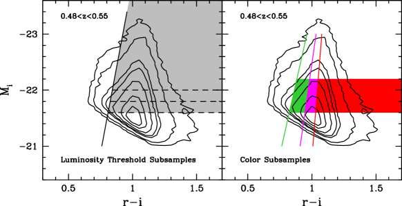
Figure 1: Left: the selection of the luminosity threshold samples in the colour-magnitude diagram (CMD). The contours represent the density distribution of the CMASS galaxies in the CMD. The shaded regions show the galaxies covered in the luminosity threshold samples. The solid line denotes the colour cut of Equation (7), and the three dashed lines represent the three luminosity thresholds. Right: the selection of the ‘green’, ‘redseq’ and ‘reddest’ colour samples in the luminosity range of $-22.2<M_{i}<-21.6$ and redshift range of $0.48<z<0.55$. The three colour solid lines are the three cuts for the fine colour samples. The green line is for the cut between the ‘blue’ and ‘green’ samples. The magenta line is the cut between the ‘green’ and ‘redseq’ samples. The red line is the cut between the ‘redseq’ and ‘reddest’ samples. The shaded regions represent our selection of the corresponding colour samples.

In this paper, we focus on modeling the luminosity and colour dependence of the CMASS red galaxies. We therefore construct suitable luminosity and colour subsamples of galaxies. Three luminosity threshold samples of red galaxies are constructed, with $M_{i}<-21.6$, $M_{i}<-21.8$, and $M_{i}<-22.0$, in the same redshift range, $0.48<z<0.55$. We use luminosity threshold samples to facilitate a more straight-forward HOD modeling of the measurements. The redshift range is selected to ensure that the red galaxies in the samples are nearly complete and minimally suffer from the selection effects (G13). Details of the samples are given in Table 1 (together with the best-fitting parameters from HOD modeling to be presented in Section 3). The left panel of Figure 1 shows the selection of the three luminosity-threshold samples in the colour-magnitude diagram (CMD). The contours represent the density distribution of the CMASS galaxies in the CMD. The solid line denotes the colour cut of Equation (7) and the shaded region and the three dashed lines show the selection of the luminosity threshold samples.

For studying the colour dependence of clustering, we divide the CMASS galaxies into ‘green’, ‘redseq’, and ‘reddest’ subsamples, using the colour cuts in Table 2 of G13. In order to have the best signal-to-noise ratio and decouple the colour dependence from the luminosity dependence, we only select galaxies in the redshift range of $0.48<z<0.55$ and luminosity range of $-22.2<M_{i}<-21.6$. The right panel in Figure 1 shows the selection of the three subsamples. The three coloured solid lines are the three cuts for the fine colour samples (G13): the green, magenta, and red lines divide the galaxies into ‘blue’, ‘green’, ‘redseq’, and ‘reddest’ subsamples, respectively. The ‘reddest’ sample has the reddest colour, while the ‘redseq’ sample represents the galaxies occupying the central part of the red sequence in the CMD. The ‘green’ sample is selected to represent the transition from blue to red galaxies. The ‘blue’ galaxy sample is not considered here because of its low completeness. More information on the colour subsamples can be found in Table 2.

2.2 Measurements of the Galaxy 2PCFs

Approximately $1.5$ per cent of CMASS galaxies in DR10 were previously observed in SDSS-II whose angular distribution differs from other BOSS galaxies (see more details in Anderson et al., 2012). The redshift measurements of these SDSS-II ‘Legacy’ galaxies are, by construction, $100$ per cent complete, while the redshift and angular completeness of BOSS galaxies vary with sky position. The different distributions of these ‘Legacy’ galaxies and the newly observed BOSS galaxies need to be carefully taken into account for clustering measurement. In previous work (e.g. Anderson et al. 2012,G13), this is achieved by subsampling the SDSS-II galaxies to match the sector completeness of BOSS survey. Here, to preserve the full information in the ‘Legacy’ galaxies, we adopt an alternative method, with a decomposition of the total 3D correlation functions as follows (Zu et al. 2008; Guo et al. 2012)

$$\xi_{T}={n_{L}^{2}\over n_{T}^{2}}\xi_{LL}+{2n_{L}n_{B}\over n_{T}^{2}}\xi_{LB}+{n_{B}^{2}\over n_{T}^{2}}\xi_{BB},$$ (8)

where $n_{L}$, $n_{B}$ and $n_{T}$ are the number densities of the Legacy, (uniquely) BOSS, and all galaxies, respectively, $\xi_{LL}$ is the auto-correlation function of Legacy galaxies, $\xi_{BB}$ is the auto-correlation function of BOSS galaxies, and $\xi_{LB}$ is the cross-correlation of Legacy and BOSS galaxies. The decomposition can be understood in terms of galaxy pair counts – the total number of galaxy pairs is composed of Legacy-Legacy pairs (related to $\xi_{LL}$), BOSS-BOSS pairs (related to $\xi_{BB}$), and the Legacy-BOSS cross-pairs (related to $\xi_{LB}$). The random samples are separately constructed for Legacy and BOSS galaxies to reflect the different angular and redshift distributions.

In galaxy surveys using fibre-fed spectrographs, the precise small-scale auto-correlation measurements are hindered by the effect that two fibres on the same plate cannot be placed closer than certain angular scales, which is $62^{\prime\prime}$ in SDSS-III, corresponding to about $0.4\,h^{-1}{\rm{Mpc}}$ at $z{\sim}0.55$. Such fibre-collision effects can be corrected by using the collided galaxies that are assigned fibres in the tile overlap regions, as proposed and tested by Guo et al. (2012) and implemented in G13.

We apply the same method here to BOSS galaxies to correct for the fibre-collision effect in measuring the 2PCFs. We divide the BOSS sample into two distinct populations, one free of fibre collisions (labelled by subscript ‘1’) and the other consisting of potentially collided galaxies (labelled by subscript ‘2’). With such a division, Equation  (8) is further decomposed into six terms as,

$$\xi_{T} = {n_{L}^{2}\over n_{T}^{2}}\xi_{LL}+{2n_{L}n_{B_{1}}\over n_{T}^{2}}\xi_{LB_{1}}+{2n_{L}n_{B_{2}}\over n_{T}^{2}}\xi_{LB_{2}}$$ (9)

$$+{n_{B_{1}}^{2}\over n_{T}^{2}}\xi_{B_{1}B_{1}}+{2n_{B_{1}}n_{B_{2}}\over n_{T}^{2}}\xi_{B_{1}B_{2}}+{n_{B_{2}}^{2}\over n_{T}^{2}}\xi_{B_{2}B_{2}}.$$

In actual measurements, the correlation functions $\xi_{LB_{2}}$, $\xi_{B_{1}B_{2}}$, and $\xi_{B_{2}B_{2}}$ involving the collided galaxies are estimated using the resolved collided galaxies in tile overlap regions (as detailed in Guo et al. 2012).

We first measure the redshift-space 2PCF $\xi(r_{p},r_{\pi})$ in bins of transverse separation $r_{p}$ and line-of-sight separation $r_{\pi}$ ($r_{p}$ in logarithmic bins from $\sim$0.02 to $\sim$63$\,h^{-1}{\rm{Mpc}}$ with $\Delta\log r_{p}=0.2$ and $r_{\pi}$ in linear bins from 0 to 100$\,h^{-1}{\rm{Mpc}}$ with $\Delta r_{\pi}=2\,h^{-1}{\rm{Mpc}}$), using the Landy & Szalay (1993) estimator. We then integrate the 2PCF along the line-of-sight direction to obtain the projected 2PCF $w_{p}(r_{p})$

$$w_{p}(r_{p})=2\int_{0}^{r_{\pi,\rm max}}\xi(r_{p},r_{\pi})dr_{\pi},$$ (10)

with $r_{\pi,\rm max}=100\,h^{-1}{\rm{Mpc}}$. This projected 2PCF is what we present and model in this paper. The covariance error matrix for $w_{p}(r_{p})$ is estimated from 200 jackknife subsamples (Zehavi et al. 2002, 2005,G13). We provide the measurements for the projected 2PCF, $w_{p}(r_{p})$, for all the subsamples used in this paper in the Appendix B. With the advantage of larger sky coverage in DR10, the correlation function measurements have much smaller errors compared with those in DR9. The measurements in DR9 and DR10 are generally consistent within the errors.

Table 2: HOD parameters for the colour samples in $-22.2<M_{i}<-21.6$

Sample	$N_{\rm gal}$	$\bar{n}(z)$	$\chi^{2}/\rm{dof}$	$\log M_{1}^{\prime}$	$f_{\rm{sat}}$(per cent)
‘green’	28835	$0.54$	20.81/16	$14.57\pm 0.04$	$3.68\pm 0.47$
‘redseq’	32221	$0.61$	15.62/18	$14.42\pm 0.03$	$6.15\pm 0.46$
‘reddest’	34670	$0.66$	35.26/18	$14.30\pm 0.02$	$9.35\pm 0.46$

The mean number density $\bar{n}(z)$ is in unit of $10^{-4}h^{3}{\rm{Mpc}}^{-3}$. The halo mass is in units of $\,h^{-1}{\rm M_{\sun}}$. The redshift range of colour samples are limited to $0.48<z<0.55$.

3 HOD modeling

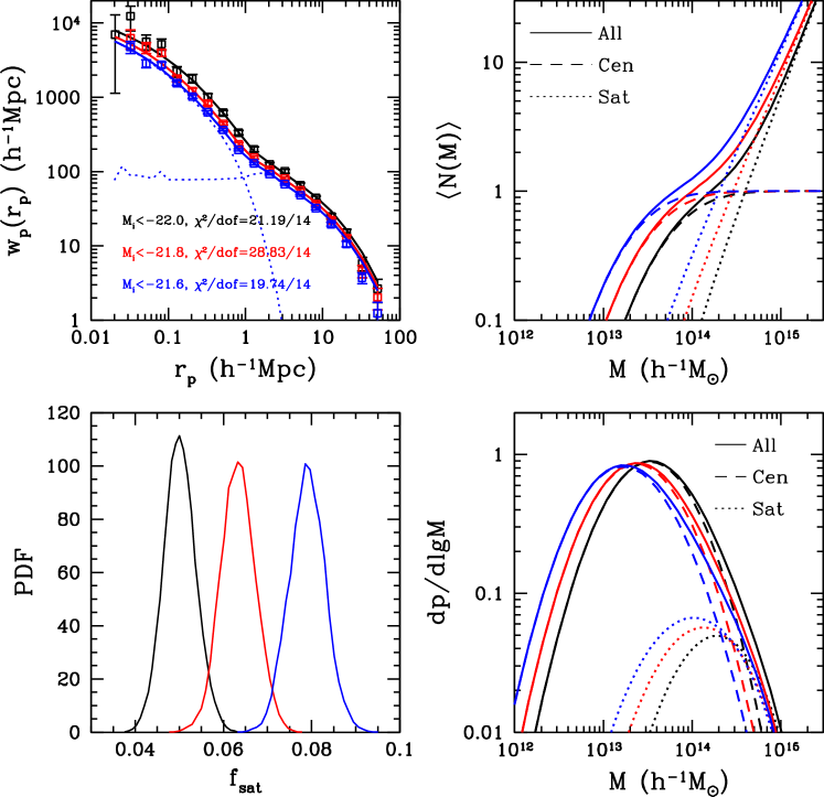
Figure 2: Projected two-point correlation functions measured in DR10 and the corresponding best-fitting HOD models for the three luminosity threshold samples. Top left: the measurements of $w_{p}(r_{p})$ from DR10 (squares) compared with the best-fitting HOD models (lines). The blue dotted lines represent the one-halo and two-halo terms for the sample of $M_{i}<-21.6$. The $\chi^{2}$ per degree of freedom (dof) for the three best-fittings are also shown. Top right: the mean occupation number distributions of the three samples. The total mean halo occupation function (solid lines) is decomposed into contributions from central galaxies (dashed lines) and satellite galaxies (dotted lines). Bottom left: The probability distribution of $f_{\rm{sat}}$. Bottom Right: The probability distribution of the host halo mass.

We perform the HOD fits to the projected two-point auto-correlation functions $w_{p}(r_{p})$, measured in different luminosity and colour bins. In the HOD framework, it is helpful to separate the contribution to the mean number $\langle N(M)\rangle$ of galaxies in halos of mass $M$ into those from central and satellite galaxies (Kravtsov et al., 2004; Zheng et al., 2005).

For luminosity-threshold samples, we follow Zheng, Coil, & Zehavi (2007) to parameterize the mean occupation functions of central and satellite galaxies as

$$\langle N_{\rm cen}(M)\rangle = {1\over 2}\left[1+{\rm erf}\left(\frac{\log M-\log M_{\rm min}}{\sigma_{\log M}}\right)\right]$$ (11)

$$\langle N_{\rm sat}(M)\rangle = \langle N_{\rm cen}(M)\rangle\left(\frac{M-M_{0}}{M_{1}^{\prime}}\right)^{\alpha}$$ (12)

where ${\rm erf}$ is the error function. In total, there are five free parameters in this parametrization. The parameter $M_{\rm min}$ describes the cutoff mass scale of halos hosting central galaxies ($\langle N_{\rm cen}(M_{\rm min})\rangle=0.5$). The cutoff profile is step-like but softened to account for the scatter between galaxy luminosity and halo mass (Zheng et al., 2005), and is characterized by the width $\sigma_{\log M}$. The three parameters for the mean occupation function of satellites are the cutoff mass scale $M_{0}$, the normalization $M_{1}^{\prime}$, and the high-mass end slope $\alpha$ of $\langle N_{\rm sat}(M)\rangle$. In halos of a given mass, the occupation numbers of the central and satellite galaxies are assumed to follow the nearest integer and Poisson distributions with the above means, respectively. In our fiducial model, the spatial distribution of satellite galaxies in halos is assumed to follow that of the dark matter, i.e. the Navarro-Frenk-White (NFW) profile (Navarro, Frenk, & White, 1997), with halo concentration parameter

$$c(M)=c_{0}(M/M_{\rm nl})^{\beta}(1+z)^{-1},$$ (13)

where $M_{\rm nl}$ is the non-linear mass scale at $z=0$, $c_{0}=11$ and $\beta=-0.13$ (Bullock et al., 2001; Zhao et al., 2009). Later in this paper, we will also consider a generalized NFW profile and use the 2PCF measurements to constrain it. Halos here are defined to have a mean density 200 times that of the background universe.

To theoretically compute the real-space 2PCF of galaxies within the HOD framework, we follow the procedures laid out in Zheng (2004) and Tinker et al. (2005). When computing the projected 2PCF from the real-space 2PCF, we also incorporate the effect of residual redshift-space distortions to improve the modeling on large scales. This is done by decomposing the 2PCF into monopole, quadrupole, and hexadecapole moments and applying the method of Kaiser (1987) (also see van den Bosch et al. 2013).

We use a Markov Chain Monte Carlo (MCMC) method to explore the HOD parameter space constrained by the projected 2PCF $w_{p}(r_{p})$ and the number density $n_{g}$ of each galaxy sample. The $\chi^{2}$ is formed as

$$\chi^{2}=\mn@boldsymbol{(w_{p}-w_{p}^{*})^{T}C^{-1}(w_{p}-w_{p}^{*})}+{(n_{g}-n_{g}^{*})^{2}\over\sigma_{n_{g}}^{2}},$$ (14)

where $\mn@boldsymbol{w_{p}}$ is the vector of $w_{p}$ at different values of $r_{p}$ and $\mn@boldsymbol{C}$ is the full error covariance matrix determined from the jackknife resampling method (as detailed in Guo et al., 2013). The measured values are denoted with a superscript ‘$*$’. The error $\sigma_{n_{g}}$ on the number density is determined from the variation of $n_{g}(z)$ in the different jackknife subsamples. Finally, in order to account for the bias introduced when inverting the covariance matrix (Hartlap, Simon, & Schneider, 2007), we multiply the above $\chi^{2}$ by a factor $(n_{jk}-n_{d}-2)/(n_{jk}-1)$, which is about 0.9 in our case. Here $n_{jk}$ is the number of jackknife samples and $n_{d}$ is the dimension of the data vector. In Appendix A, we demonstrate the robustness and accuracy of our fitting with jackknife covariance matrices by comparing with results from using mock covariance matrices.

4 Modeling Results

4.1 HOD for the Luminosity-threshold Samples

Figure 3: Two mass scales in HOD models as a function of threshold luminosity of the galaxy samples, where $\langle N_{\rm cen}(M_{\rm min})\rangle=0.5$ and $\langle N_{\rm sat}(M_{1})\rangle=1$. The squares and solid lines are the HOD modeling results of the three luminosity threshold samples, while the dashed line shows the relation of $M_{1}{\sim}8.7M_{\rm min}$.

The best-fitting HOD parameters for the three luminosity threshold samples are listed in Table 1. Figure 2 shows the modeling results. The top-left panel displays the measurements of $w_{p}(r_{p})$ in DR10 (squares) compared with the best-fitting HOD models (lines). The top-right panel shows the mean occupation functions from the three best-fitting models. Overall, the trend of stronger clustering for more luminous CMASS samples is explained in the HOD framework as a shift toward higher mass scale of host halos, similar to that for the SDSS MAIN galaxies (Zehavi et al., 2011).

The mean occupation functions in the top-right panel also show that a fraction of the CMASS luminous red galaxies must be satellites in massive halos. This is required to fit the small-scale clustering. The probability distribution of $f_{\rm{sat}}$ is shown in the bottom-left panel of Figure 2. More luminous galaxies have a lower fraction of satellites, consistent with the trend found for MAIN sample galaxies (Zehavi et al., 2011) and luminous red galaxies (Zheng et al., 2009). The peak $f_{\rm{sat}}$ varies from $8$ per cent for the $M_{i}<-21.6$ sample to $5$ per cent for the $M_{i}<-22.0$ sample.

The bottom-right panel of Figure 2 shows the probability distributions of host halo mass for the three samples, generated from the product of the mean occupation function and the differential halo mass function (Wake et al., 2008; Zheng et al., 2009). The host halos refer to the main halos, i.e. we do not consider the subhalos as the host halos. Most of the central galaxies in these samples reside in halos of about a few times $10^{13}\,h^{-1}{\rm M_{\sun}}$, while the satellite galaxies are mostly found in halos of masses around ${\sim}10^{14}\,h^{-1}{\rm M_{\sun}}$. More luminous galaxies have a higher probability to be found in more massive halos. For central galaxies, in the narrow luminosity range in our samples, the peak host halo mass varies from $1.1\times 10^{13}$ to $3.3\times 10^{13}\,h^{-1}{\rm M_{\sun}}$ for the three samples.

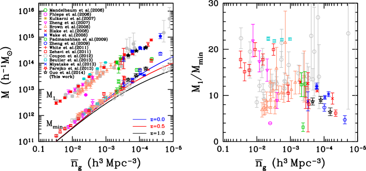
Figure 4: Left panel: HOD parameters $M_{\rm min}$ (open symbols) and $M_{1}$ (solid symbols) as a function of the average number density $\bar{n}_{g}$ of the samples. Different symbols represent the measurements from the literature, as labelled in the figure. Our measurements of the three luminosity threshold samples are displayed by the black stars, which are in good agreement with the literature. The halo mass functions at the three typical redshifts $z=0$, $0.5$, and $1$ are also shown as the solid lines. Right panel: the ratio between $M_{1}$ and $M_{\rm min}$ for all the measurements in literature.

Figure 3 displays the relation of the HOD parameters $M_{\rm min}$ and $M_{1}$ with the threshold luminosity $M_{i}$. Note that the quantity $M_{\rm min}$ is the characteristic mass of halos hosting central galaxies at the threshold luminosity (with $\langle N_{\rm cen}(M_{\rm min})\rangle=0.5$), and $M_{1}$ is the characteristic mass of halos hosting on average one satellite galaxy above the luminosity threshold ($\langle N_{\rm sat}(M_{1})\rangle=1$), which has a subtle difference from $M_{1}^{\prime}$. Clearly, the tight correlation between galaxy luminosity and halo mass scales persists for massive galaxies in massive halos at $z\sim 0.5$. The scaling relation between $M_{\rm min}$ and $M_{1}$ in our samples roughly follows $M_{1}{\sim}8.7M_{\rm min}$. The large gap between $M_{1}$ and $M_{\rm min}$ implies that a halo with mass between $M_{\rm min}$ and $M_{1}$ tends to host a more massive central galaxy rather than multiple smaller galaxies (Berlind et al., 2003). This $M_{1}$-to-$M_{\rm min}$ ratio is comparable to the one found for SDSS LRGs (Zheng et al., 2009) and significantly smaller than the scaling factor found for the SDSS MAIN galaxies ($\sim 17$, Zehavi et al. 2011). The ratio decreases somewhat with increasing luminosity – for the most luminous sample we analyse ($M_{i}<-22.0$), the ratio is $6.4^{+0.5}_{-0.4}$, smaller than the ${\sim}8.7$ inferred from the lower luminosity-threshold samples. Such a trend with luminosity is also found in other SDSS analyses (Zehavi et al., 2005, 2011; Skibba, Sheth, & Martino, 2007; Zheng et al., 2009). These behaviors are likely related to the dominance of accretion of satellites over destruction in massive halos. More massive, cluster-sized halos form late and accrete satellites more recently, leaving less time for satellites to merge onto the central galaxies and thus lowering the satellite threshold mass $M_{1}$ (Zentner et al., 2005).

In Figure 4 we compare the measurements of $M_{\rm min}$ and $M_{1}$ of our samples with those from the literature of various surveys (Mandelbaum et al., 2006; Phleps et al., 2006; Kulkarni et al., 2007; Zheng, Coil, & Zehavi, 2007; Brown et al., 2008; Blake, Collister, & Lahav, 2008; Wake et al., 2008; Padmanabhan et al., 2009; Zheng et al., 2009; White et al., 2011; Zehavi et al., 2011; Coupon et al., 2012; Beutler et al., 2013; Miyatake et al., 2013; Parejko et al., 2013). We plot them as a function of galaxy number density $\bar{n}_{g}$ (note that a lower $\bar{n}_{g}$ corresponds to a higher threshold in galaxy luminosity or stellar mass). The mass scales are all corrected to the cosmology adopted in this paper according to their proportionality to $\Omega_{m}$ (Zheng et al., 2002, 2009). The left panel shows $M_{\rm min}$ (open symbols) and $M_{1}$ (solid symbols) as a function of (decreasing) number density of the different samples. The right panel displays the corresponding ratios $M_{1}/M_{\rm min}$. Our results of the three luminosity threshold samples (black stars) are in good agreement with the trend shown in other samples.

Brown et al. (2008) noted that $M_{\rm min}$ and $\bar{n}_{g}$ approximately follow a power-law relation with a power-law index ${\sim}-1$. Such a power-law relation can be largely explained from the the halo mass function. In the left panel, we plot the cumulative halo mass functions $n_{h}(>M)$ at three typical redshifts, $z=0$, 0.5, and 1, as solid curves. The halo mass functions are analytically computed for the assumed cosmological model. The low-mass end ($M<10^{12}\,h^{-1}{\rm M_{\sun}}$) of the halo mass function closely follows $n_{h}(>M)\propto M^{-1}$ and evolves slowly with redshift. At the high-mass end, the halo mass function drops more rapidly than the power-law at the low mass end, and shows stronger redshift evolution. The halo mass function $n_{h}(M>M_{\rm min})$ can be regarded as resulting from a simple form of HOD — one galaxy per halo and a sharp cutoff at $M_{\rm min}$, i.e. $\langle N(M)\rangle=1$ for $M>M_{\rm min}$ and 0 otherwise, where $M_{\rm min}$ is determined by matching the galaxy number density. Thus, any deviation from the halo mass function curves could only be caused by the existence of satellite galaxies and the softened mass cutoff around $M_{\rm min}$ for central galaxies. For high number density galaxy samples, the deviation arises from the satellite galaxies, since these halos have large satellite fractions (see Figure 5). For low number density samples, the prominent deviation is mainly a result of the wide softened cutoff in the central galaxy mean occupation function. Such a wide softened cutoff is a manifestation of the large scatter between central galaxy luminosity and halo mass (Zheng et al. 2007). It is interesting that the deviations at both the low- and high-mass end drive the $M_{\rm min}$–$\bar{n}_{g}$ relation towards a power law.

The $M_{1}$–$\bar{n}_{g}$ relation also roughly follows a power law with a slightly shallower slope than the $M_{\rm min}$–$\bar{n}_{g}$ relation. As a consequence, there is a trend that the ratio $M_{1}/M_{\rm min}$ decreases with decreasing $\bar{n}_{g}$, albeit with a large scatter, as shown in the right panel of Figure 4. This result is consistent with what we find in the luminosity dependence of $M_{1}/M_{\rm min}$.

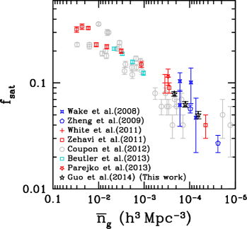
Figure 5: Satellite fraction $f_{\rm{sat}}$ as a function of the average number density $\bar{n}_{g}$ of the samples. Different symbols represent the measurements from the literature, as labelled in the figure. Our measurements of the three luminosity threshold samples are displayed by the black stars.

Figure 5 presents the satellite fraction $f_{\rm{sat}}$ as a function of the number density $\bar{n}_{g}$ from our luminosity-threshold samples and those from the literature. The satellite fraction appears to follow a well-defined sequence, especially toward low number density, declining with decreasing number density and can be well described by a power law, $f_{\rm sat}\simeq 0.1[\bar{n}_{g}/(10^{-3}h^{3}{\rm Mpc}^{-3})]^{1/3}$.

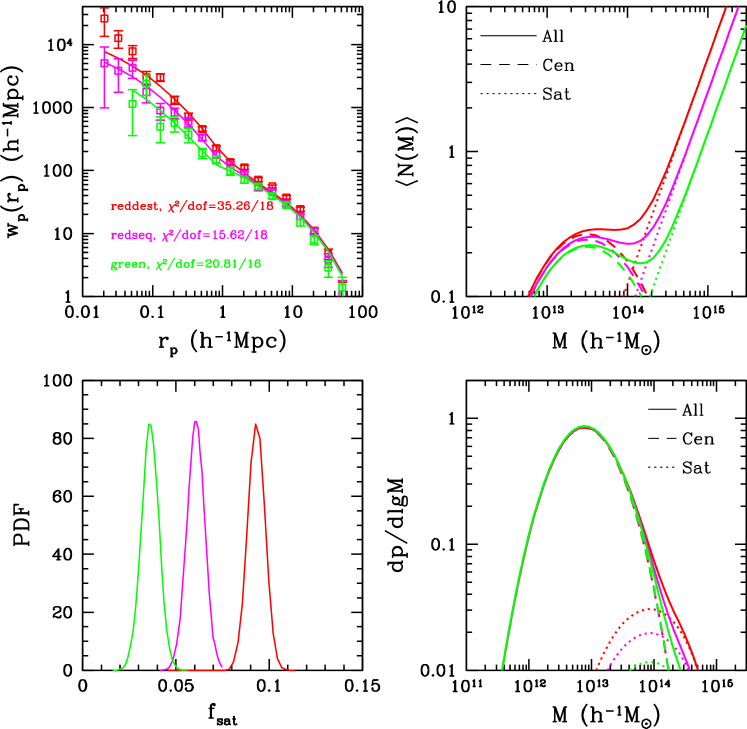
Figure 6: Similar to Figure 2, but for the different colour samples in the luminosity range $-22.2<M_{i}<-21.6$ and redshift range $0.48<z<0.55$. The red, magenta, and green lines are for the ‘reddest’, ‘redseq’ and ‘green’ samples, respectively.

4.2 HOD for the Colour Samples

To model the colour dependence of the 2PCFs for the CMASS galaxies in the luminosity bin of $-22.2<M_{i}<-21.6$, we form the mean occupation function of the central galaxies in this luminosity bin as the difference between $\langle N_{\rm cen}(M)\rangle$ of the $M_{i}<-21.6$ sample and that of the $M_{i}<-22.2$ sample. Following Zehavi et al. (2011), we fix the slope $\alpha$ of the satellite mean occupation function to be 1.56, the value from the fainter luminosity threshold sample that dominates the number density of the luminosity-bin sample. The cutoff mass of the mean occupation function of satellite galaxies is also set to be the smaller of the two values from the two threshold samples. Thus, we model the 2PCF of each colour subsample with only one free parameter, $M_{1}^{\prime}$. In this simple model, the shape of the central or satellite mean occupation functions for different colour samples remains the same, and the relative normalization between the central and satellite mean occupation functions is governed by $M_{1}^{\prime}$ and constrained by the small-scale clustering. The overall normalizations of the mean occupation functions are determined from the relative number densities of the colour samples to the total number density in this luminosity bin. By construction, the sum of the mean galaxy occupation functions of all colour samples (including the ‘blue’ galaxies that are not modeled in this paper) equals that of the full luminosity-bin sample.

Figure 6 shows the modeling result (also in Table 2) of the three colour samples, in a similar format to that of Figure 2. It is evident from the figure that redder galaxies have a higher clustering amplitude, especially on small scales (one-halo term). Within our model, the higher clustering amplitude in the redder galaxies is a result of a larger fraction of them being satellites (in massive halos), as shown in the top-right and bottom-left panels. The satellite fraction $f_{\rm sat}$ varies from $3.7$ per cent in the ‘green’ sample to $9.4$ per cent in the ‘reddest’ sample, consistent with the trend in MAIN sample (Zehavi et al., 2005, 2011). Compared with the luminosity dependence of galaxy clustering, where more luminous galaxies reside in more massive halos and have smaller satellite fractions, the trend in the colour dependence indicates that the satellite fraction mostly affects the small-scale clustering, while halo mass scales affect the overall clustering amplitudes (especially on large scales dominated by the two-halo term).

The top-left panel of Figure 6 demonstrates that the projected 2PCF of the ‘reddest’ sample on small scales ($r_{p}<0.2\,h^{-1}{\rm{Mpc}}$) is not well fitted by the simple HOD model, leading to a high value of best-fitting $\chi^{2}$. Even if we allow the slope $\alpha$ of the mean satellite occupation function to vary, the situation does not significantly improve. We explore the implication for the small-scale galaxy distribution inside halos with a generalized NFW profile in Section 4.3.

A close inspection of the best-fitting projected 2PCFs in the top-left panel shows that the model predicts a narrower range of clustering amplitude than that from the data on scales above a few $\,h^{-1}{\rm{Mpc}}$. Since the large-scale amplitude in the 2PCF is mainly determined by central galaxies, this result implies that the halo mass scales for central galaxies in the luminosity bin can vary with the colour to some degree (in the sense of higher mass scales for redder central galaxies) in a manner that is not captured in our simple model.

4.3 Generalized NFW profile

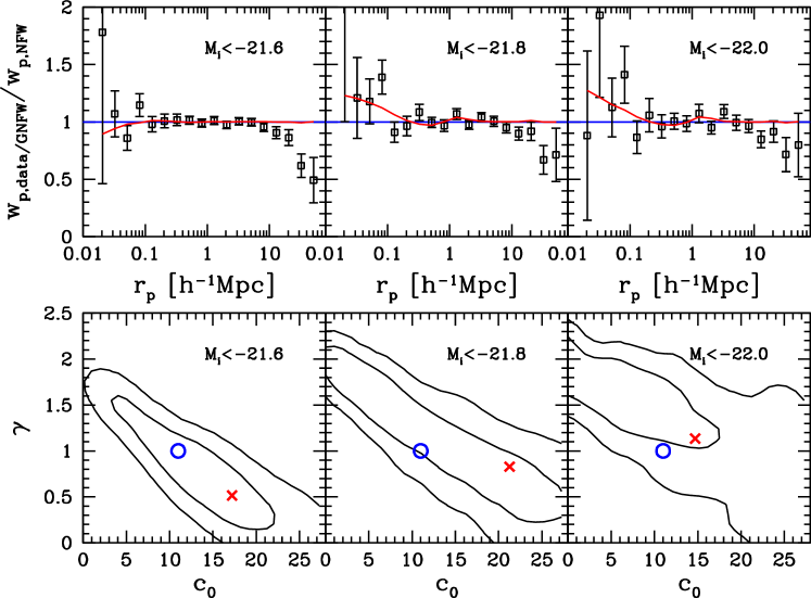
Figure 7: Top panels: ratios of $w_{p}(r_{p})$ predicted from the best-fitting GNFW HOD models and those measured from the data to those of the NFW model predictions. The black squares represent the data measurements, while the red lines are the predictions of the GNFW models. Bottom panels: marginalized joint distribution of the concentration parameter $c_{0}$ and the slope $\gamma$ in the generalized NFW model for the three luminosity threshold samples. The contours show the $68$ per cent and $95$ per cent confidence levels for the two parameters. The red crosses represent the best-fitting GNFW HOD models, while the blue circles are the predictions of the NFW model.

In our fiducial HOD model, we assume that the spatial distribution of satellite galaxies inside halos follows the same NFW profile as the dark matter. The best-fitting small-scale clustering amplitude for the ‘reddest’ sample shows deviations from the data (see Figure 6), implying a possible departure of the satellite distribution from the NFW profile. To explore such a possibility, we also consider a generalized NFW (hereafter GNFW) profile to describe the distribution of satellite galaxies inside halos by allowing two more free parameters in the HOD model, the normalization parameter $c_{0}$ for the halo concentration in Equation (13) and the slope $\gamma$ in the density profile (Watson et al., 2010, 2012; van den Bosch et al., 2013),

$$\rho(r)\propto\left[\left({c\,r\over r_{\rm vir}}\right)^{\gamma}\left(1+{c\,r\over r_{\rm vir}}\right)^{3-\gamma}\right]^{-1}$$ (15)

where $r_{\rm vir}$ is the virial radius of the halo. As a special case, the NFW profile has $c_{0}=11$ (Equation 13) and $\gamma=1$. Another special case is the singular isothermal sphere (SIS) distribution, which has $c_{0}\rightarrow 0$ and $\gamma=2$.

Table 3: $\chi^{2}/\rm{dof}$ in generalized NFW models

Sample	$\chi^{2}/\rm{dof}$	$\Delta\rm{AIC}$	$\exp(\Delta\rm{AIC}/2)$	$f_{\rm{sat}}(\rm{per\,cent})$
$M_{i}<-21.6$	$19.34/12$	3.60	6.05	$7.76\pm 0.55$
$M_{i}<-21.8$	$24.75/12$	-0.08	0.96	$5.77\pm 0.55$
$M_{i}<-22.0$	$18.93/12$	1.74	2.39	$4.66\pm 0.56$
‘green’	17.84/14	1.03	1.67	$4.11\pm 0.53$
‘redseq’	11.76/16	0.14	1.07	$6.50\pm 0.61$
‘reddest’	28.94/16	-2.32	0.31	$9.73\pm 0.62$

$\Delta\rm{AIC}=\rm{AIC_{GNFW}}-\rm{AIC_{NFW}}$

We first apply the GNFW model to the luminosity-threshold samples. From Figure 2, the HOD model using the NFW profile can fit the 2PCFs of the luminosity-threshold samples reasonably well. By including the two additional free parameters, the best-fitting $\chi^{2}$ values only decrease slightly, as shown in Table 3. To compare the goodness of fits between the generalized and original NFW profiles, we make use of the Akaike information criterion (AIC; Akaike, 1974), defined as ${\rm AIC}=\chi^{2}+2k$ for each model, where $k$ is the number of HOD parameters. The difference $\Delta{\rm AIC}\equiv\rm{AIC_{GNFW}}-\rm{AIC_{NFW}}$ between the AIC values of the GNFW and NFW models reveals that the model with the NFW profile is $\exp(\Delta\rm{AIC}/2)$ times as probable as that with the GNFW profile. As shown in Table 3, only the $M_{i}<-21.8$ sample shows a marginal preference for the GNFW profile. Overall, the clustering data of the luminosity-threshold samples do not require a profile different than the NFW profile.

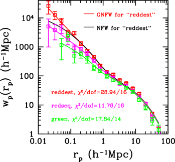
Figure 8: The same measurements of Figure 6, but now with the GNFW best-fitting models. The red, magenta, and green lines are for the ‘reddest’, ‘redseq’ and ‘green’ samples, respectively. For comparison, we also show the best-fitting NFW model for the ‘reddest’ sample as the black line.

To present a detailed examination of the effect of the GNFW profile, we show in the top panels of Figure 7 the ratios of $w_{p}(r_{p})$ predicted from the best-fitting GNFW HOD models (red lines) and the measured $w_{p}(r_{p})$ (squares) to those of the NFW model predictions. Both the NFW and GNFW models fit the data reasonably well on scales of $r_{p}<10\,h^{-1}{\rm{Mpc}}$. Their predictions are similar on large scales and they only differ slightly on scales below $\sim$1$\,h^{-1}{\rm{Mpc}}$. On larger scales, the models appear to overestimate the large scale bias for all samples, which might be caused by the sample variance.

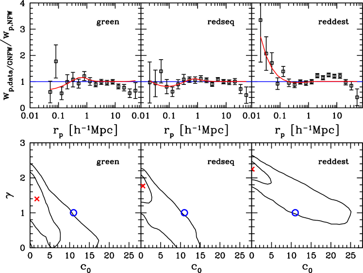
Figure 9: Similar to Figure 7, but for the three colour samples in the luminosity bin $-22.2<M_{i}<-21.6$.

The marginalized joint distribution of the concentration normalization $c_{0}$ and the slope $\gamma$ for the three luminosity threshold samples are shown in the bottom panels of Figure 7. The best-fitting models are displayed as the red crosses and the NFW model is represented by the blue circles. While there is a weak trend that the profile for more luminous samples prefers to deviate from the NFW profile, the NFW profile is still within the $\sim 2\sigma$ range of the contours. Watson et al. (2010) and Watson et al. (2012) find that the distributions of satellite LRGs and satellites of luminous galaxies in SDSS MAIN sample have significantly steeper inner slopes than the NFW profile. From Figure 1 in both Watson et al. (2010) and Watson et al. (2012), we infer that constraining the deviation from the NFW profile requires accurate measurements on scales $r_{p}<0.03\,h^{-1}{\rm{Mpc}}$. However, at such small scales, the effect of photometric blending of close pairs may be important in clustering measurements (Masjedi et al., 2006; Jiang, Hogg, & Blanton, 2012), which is not corrected for in our samples. Moreover, the measurement errors at these scales are large in our samples. We therefore can only conclude that our measurements and modeling results show no strong deviations from the NFW profile in the distribution of satellites inside halos for luminosity-threshold samples.

We then apply the GNFW model to the fine colour samples in Section 4.2. Significant improvement over the NFW profile model is found in fitting the small-scale 2PCF of the ‘reddest’ sample, as shown in Figure 8. Without the variation in $c_{0}$ and $\gamma$, the pure NFW model cannot fit well the small-scale clustering by only adjusting the satellite fraction or the slope $\alpha$ of the satellite mean occupation function. The best-fitting $\chi^{2}$ value for this colour sample is also reduced by adding the two free parameters, as shown in Table 3. From the difference in the AIC, the NFW model is much less favorable than the GNFW model for the ‘reddest’ sample, while it still provides reasonable fits to the ‘green’ and ‘redseq’ samples.

The ratios of the HOD model predictions of GNFW models and the measured $w_{p}(r_{p})$ to those of the NFW model are shown in the top panels of Figure 9. The small-scale clustering of the ‘reddest’ sample is better fit by the GNFW model, which confirms the importance of the small-scale ($r_{p}<0.1\,h^{-1}{\rm{Mpc}}$) measurements in distinguishing the NFW and GNFW models. The marginalized joint distribution of $c_{0}$ and $\gamma$ is presented in the bottom panels of Figure 9. From the $1\sigma$ contours of Figure 9, there is a visible trend that redder galaxies favor smaller $c_{0}$ and larger $\gamma$. The SIS profile (corresponding to $c_{0}\rightarrow 0$ and $\gamma=2$) seems to provide better fits than the NFW profile, consistent with the previous findings (Grillo, 2012; Watson et al., 2012). This trend is clearly manifested for the ‘reddest’ sample.

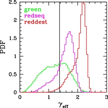
Figure 10: Probability distributions of the effective slope $\gamma_{\rm eff}$ at $r=0.1\,h^{-1}{\rm{Mpc}}$ in halos of $2\times 10^{14}\,h^{-1}{\rm M_{\sun}}$ for the three colour samples. The vertical black line denotes $\gamma_{\rm eff}=1.37$, the value for the NFW profile at this radius.

Since $c_{0}$ and $\gamma$ are correlated, different combinations of them can lead to similar shape of the profile. A better quantity to represent the shape of the density profile is the effective slope defined as

$$\gamma_{\rm eff}\equiv-\frac{d\ln\rho(r)}{d\ln r}=\gamma+\frac{c(3-\gamma)}{c+r_{\rm vir}/r}.$$ (16)

It is the local slope of the profile at radius $r$ for halos of virial radius $r_{\rm vir}$. That is, if approximated by a power law, the local profile is proportional to $r^{-\gamma_{\rm eff}}$. To understand the trend shown in Figure 9 for the three colour samples, we show in Figure 10 the probability distributions of the effective slope $\gamma_{\rm eff}$ at $r=0.1\,h^{-1}{\rm{Mpc}}$ in halos of $2\times 10^{14}\,h^{-1}{\rm M_{\sun}}$. For reference, the vertical black line denotes the $\gamma_{\rm eff}$ for the NFW profile at the same radius. There is a clear trend that the distribution of redder galaxies has a steeper effective slope, as expected from the top panels of Figure 9. While the effective slopes for the ‘green’ and ‘redseq’ galaxies still agree with the NFW model, that for the ‘reddest’ colour sample deviates significantly from the NFW value. The above model assumes a fixed slope $\alpha$ for $\langle N_{\rm sat}\rangle$. If we allow $\alpha$ to vary, each probability distribution curve in Figure 10 becomes broader (as well as the range given by the contours in Figure 9), but the trend remains the same and the result is still valid. We therefore conclude that the steep rise in the small-scale 2PCF of the ‘reddest’ colour sample favors a GNFW profile with a steeper inner slope.

4.4 Central-Satellite Correlation

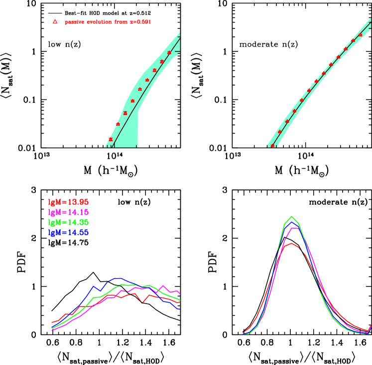
Figure 11: Top panels: satellite occupation distributions for the low and moderate $n(z)$ samples. The solid lines are the best-fitting HOD models at $z=0.512$ and the green shaded areas are the $1\sigma$ distribution. The triangles are the mean occupation function obtained by using the simulations to passively evolve the best-fitting $z=0.591$ HOD to $z=0.512$. Bottom panels: probability distributions of the ratios between the satellite occupation numbers of the passively evolved HOD and the best-fitting HOD. Different colour lines correspond to different host halo masses.

For the HOD model in previous sections, we make an implicit and subtle assumption in the one-halo central-satellite galaxy pairs, related to the correlation between central and satellite galaxies. For the contribution of the one-halo central-satellite galaxy pairs in the model, one needs to specify the mean $\langle N_{\rm cen}N_{\rm sat}\rangle$ at each halo mass. We compute it as $\langle N_{\rm cen}N_{\rm sat}\rangle=\langle N_{\rm sat}\rangle$. This result implies that for a given galaxy sample, a halo hosting a satellite galaxy also hosts a central galaxy from the same sample (Zheng et al., 2005; Simon et al., 2009). Such an assumption is quite reasonable for luminosity-threshold samples, if the central galaxy is the most luminous galaxy in a halo. However, for a luminosity-bin sample or colour subsamples, a scenario can arise where the central galaxy in a halo hosting satellite galaxies from the sample does not itself belong to the sample.

To explore the effect of the central-satellite correlation, we consider an extreme case in which the occupations of central and satellite galaxies inside halos are completely independent, i.e. the probability of a halo to host a satellite does not depend on whether it has a central galaxy from the same sample. The mean number of central-satellite pairs is then computed as $\langle N_{\rm cen}N_{\rm sat}\rangle=\langle N_{\rm cen}\rangle\langle N_{\rm sat}\rangle$.

Table 4: HOD Model Fitting Results for independent Central-Satellite Distribution

Sample	$({\chi^{2}\over\rm{dof}})_{\rm{NFW}}$	$({\chi^{2}\over\rm{dof}})_{\rm{GNFW}}$	$f_{\rm{sat,NFW}}$	$f_{\rm{sat,GNFW}}$
$M_{i}<$-21.6	$21.89/14$	$19.38/12$	$9.92\pm 0.55$	$8.88\pm 0.73$
$M_{i}<$-21.8	$33.02/14$	$25.14/12$	$8.26\pm 0.59$	$6.93\pm 0.78$
$M_{i}<$-22.0	$22.56/14$	$18.69/12$	$6.95\pm 0.71$	$3.98\pm 1.17$
‘green’	22.17/16	21.59/14	$7.02\pm 0.50$	$6.90\pm 0.73$
‘redseq’	14.52/18	12.88/16	$10.14\pm 0.60$	$10.03\pm 0.59$
‘reddest’	52.26/18	24.26/16	$12.98\pm 0.52$	$13.20\pm 0.50$

$f_{\rm{sat}}$ is in unit of per cent.

Table 4 summarizes the HOD modeling results for independent central-satellite occupations. The general results and trends stay similar to those previously discussed. Compared with the fitting results obtained in the previous sections, the satellite fractions are somewhat increased, with the increase for the colour samples more substantial (a factor of 1.4–1.9). The change in satellite fraction is expected: for $\langle N_{\rm cen}\rangle<1$ halos, the central-satellite independent case has a lower number of central-satellite pairs per halo compared to our fiducial case, which would predict weaker small-scale clustering; the model compensates this by having a higher $\langle N_{\rm sat}\rangle$. The $\chi^{2}$ values are, however, generally similar to the previous results, which implies that the current data are not able to put strong constraints on the correlation between central and satellite galaxies.

The exact level of the correlation between central and satellite galaxies is determined by galaxy formation physics. As discussed in Zentner, Hearin, & van den Bosch (2013), it may be related to the formation history of the dark matter halos, exhibiting assembly bias (e.g. Gao et al., 2005), and it may be further enhanced by the phenomenon of “galactic conformity” (e.g. Weinmann et al., 2006). For the galaxy samples considered in this work, the host halo masses are about two orders of magnitude higher than the non-linear mass scale at $z\sim 0.5$, and the halo assembly bias for such massive halos is expected to be small (e.g. Wechsler et al., 2006; Jing, Suto, & Mo, 2007). In any case, our simple exercise here gives us some idea on the magnitude of the uncertainty in the modeling results (e.g. the satellite fraction) caused by potential galaxy/halo assembly bias.

4.5 Evolution of Satellite Galaxies

HOD modeling results at different redshifts can be used to study galaxy evolution (e.g. Zheng, Coil, & Zehavi, 2007; White et al., 2007). In order to study the evolution of the LRGs in CMASS, we follow Guo et al. (2013) and consider samples of constant space number density from high to low redshifts, which allow for more direct comparison with predictions of passive evolution. We construct two samples with $n(z)=0.4\times 10^{-4}\,h^{3}\rm{Mpc}^{-3}$ (denoted as ‘low $n(z)$’ sample) and $n(z)=1.2\times 10^{-4}\,h^{3}\rm{Mpc}^{-3}$ (denoted as ‘moderate $n(z)$’ sample), respectively, using redshift-dependent luminosity thresholds. We consider the evolution between two redshift ranges of $0.566<z<0.616$ ($\bar{z}=0.591$) and $0.487<z<0.537$ ($\bar{z}=0.512$). The redshifts are selected to ensure the completeness of the LRG samples as well as to match the simulation outputs (see below). The median redshifts of galaxies in these two redshift ranges are only slightly different from the simulation outputs since we are considering narrow redshift intervals of $\Delta z=0.05$, therefore the choices of the redshift ranges do not affect our conclusions.

In Guo et al. (2013), based on the evolution of large-scale bias factors, we showed that the evolution of fixed number-density samples is consistent with passive evolution (Fry, 1996). Such a simple model is not sensitive to the evolution of satellites. Here we follow a similar method as in White et al. (2007) (see also Seo, Eisenstein, & Zehavi 2008) to study the evolution of satellite galaxies. For each constant number density sample, we perform HOD modeling at the two redshifts and infer the corresponding HODs. We then populate halos identified at $z=0.591$ (high-$z$) in an $N$-body simulation based on the high-$z$ HOD solutions, by using particles to represent galaxies. These particles are tracked in the simulation to $z=0.512$ (low-$z$) to derive the passively evolved HOD. In such a passive evolution, each galaxy keeps its own identity and there is no merging and disruption. The difference between the passively evolved HOD and the HOD inferred from the low-$z$ clustering then allows us to study galaxy evolution.

We use a set of 16 simulations from Jing, Suto, & Mo (2007), which employ $1024^{3}$ particles of mass $1.5\times 10^{10}\,h^{-1}{\rm M_{\sun}}$ in a periodic box of $600\,h^{-1}{\rm{Mpc}}$ on a side (detailed in Jing et al. 2007). The cosmological parameters in the simulations are $\Omega_{m}=0.268$, $\Omega_{\Lambda}=0.732$, $h=0.71$, $\Omega_{b}$=0.045, and $\sigma_{8}=0.85$. The primordial density field is assumed to be a Gaussian distribution with a scale-invariant power spectrum. The linear power spectrum is described using the transfer function of Eisenstein & Hu (1998). To be consistent, we adopt this cosmology for the 2PCF measurements and HOD modeling in this subsection. For each fixed number density sample, we populate $z=0.591$ halos using the corresponding best-fitting HOD and track the ‘galaxies’ to $z=0.512$. We then compare these passive evolution predictions with the best-fitting HOD model at this lower redshift. The results for the mean satellite occupation functions are presented in the top panels of Figure 11. In each panel, the solid curve is the best-fitting HOD model at $\bar{z}=0.512$ with the shaded area showing the $1\sigma$ distribution around the best-fitting model. The triangles are the passive evolution predictions from the simulation. The evolution of the constant $n(z)$ samples generally agrees with the passive evolution predictions, although the low-$n(z)$ sample shows a slight deviation at the low-mass end.

To fully explore the evolution of the satellite galaxies, we also must take into account the uncertainty in the high-redshift HOD models. For this purpose, we randomly select $10,000$ models from the MCMC chains at $z=0.591$ and passively evolve them (by tracking the particles in the simulations) to $z=0.512$. We then derive the mean satellite occupation numbers of the $10,000$ models, which we denote as $\langle N_{\rm sat,passive}\rangle$, at each halo mass. We also randomly select $10,000$ models from the MCMC chains at $z=0.512$ and denote their mean satellite occupation number as $\langle N_{\rm sat,HOD}\rangle$. We calculate from all of these models the distribution of the ratio $\langle N_{\rm sat,passive}\rangle/\langle N_{\rm sat,HOD}\rangle$, which is shown in the bottom panels of Figure 11, colour-coded for satellites in halos of different masses. If galaxies only evolve passively, the ratio should be one. Given the broad distribution of the $\langle N_{\rm sat,passive}\rangle/\langle N_{\rm sat,HOD}\rangle$ ratio, our results are consistent with satellite galaxies in both samples experiencing no substantial merging or disruption during the above redshift interval.

White et al. (2007) study the evolution of LRGs from $z{\sim}0.9$ to $z{\sim}0.5$ in the NOAO Deep Wide-Field Survey (NDWFS; Jannuzi & Dey, 1999) and find that about one third of the luminous satellite galaxies in massive halos appear to undergo merging or disruption in this redshift range. The average merger/disruption rate per Gyr is about $14$ per cent. Assuming the same merger/disruption rate in our smaller redshift range, which spans about 0.5 Gyr, the expected total merger/disruption rate of the satellite galaxies would be about $7$ per cent. Wake et al. (2008) also study the evolution of LRGs from redshift $z=0.55$ to $z=0.19$, and find an average merger rate of $2.4$ per cent per $\rm{Gyr}$. Given the large uncertainty in the distributions seen in the bottom panels of Figure 11, our results are not inconsistent with those in White et al. (2007) and Wake et al. (2008). A larger redshift interval would help to reduce the statistical uncertainties and allow better constraints on the evolution of galaxies, which we will consider in future work.

5 Conclusion

In this paper, we perform HOD modeling of projected 2PCFs of CMASS galaxies in the SDSS-III BOSS DR10, focusing on the dependence on galaxy colour and luminosity. We study the relation of galaxies to dark matter halos, interpret the trends with colour and luminosity, and investigate the implications for galaxy distribution inside halos and galaxy evolution.

The galaxy-halo relations from our three luminosity threshold samples show trends consistent with those in the SDSS MAIN and LRG samples (Zehavi et al., 2005, 2011; Zheng et al., 2009). The tight correlation between galaxy luminosity and halo mass persists for luminous galaxies in massive halos at $z\sim 0.5$. More luminous galaxies occupy more massive halos, with most of galaxies in our samples residing in halos of $10^{13}$–$10^{14}\,h^{-1}{\rm M_{\sun}}$ as central galaxies. The fraction of satellite galaxies decreases with galaxy luminosity threshold, varying from $\sim 8$ per cent for $M_{i}<-21.6$ galaxies to $\sim 5$ per cent for $M_{i}<-22.0$ galaxies. Most of the satellite galaxies reside in halos of mass $\sim 10^{14}\,h^{-1}{\rm M_{\sun}}$.

For the characteristic halo mass scales $M_{\rm min}$ and $M_{1}$ for central and satellite galaxies, respectively, the gap between them is smaller for more luminous galaxies, again consistent with the findings for the SDSS MAIN sample (Zehavi et al., 2005, 2011). The ratio $M_{1}/M_{\rm min}$ for CMASS galaxies is about $8.7$, significantly smaller than the ${\sim}17$ ratio for the fainter MAIN sample galaxies (Zehavi et al., 2011), but similar to that for LRGs (Zheng et al., 2009). The smaller $M_{1}/M_{\rm min}$ ratio implies a more recent accretion of luminous satellite galaxies in massive halos.

For the three colour subsamples studied, in the luminosity range of $-22.2<M_{i}<-21.6$ and redshift range of $0.48<z<0.55$, redder galaxies exhibit stronger clustering amplitudes and steeper slopes of the projected 2PCFs on small scales, while the large-scale clustering is similar. We interpret the colour trend with a simple HOD model where the three samples all have their central galaxies in halos of the same mass range (around $10^{13}\,h^{-1}{\rm M_{\sun}}$), but the satellite fraction is higher for redder galaxies (see Zehavi et al. 2011). A higher satellite fraction for redder galaxies enhances the contribution from small-scale pairs, resulting in stronger small-scale clustering. On large scales, the 2PCF is dominated by the central galaxies contribution, and the similar halo mass scales for central galaxies therefore lead to similar large-scale clustering amplitudes.

The accurate fibre-collision correction (Guo et al. 2012) enables a measurement of the 2PCFs on small scales (below $\sim 0.4\,h^{-1}{\rm{Mpc}}$), providing an opportunity to constrain the small-scale distribution of galaxies within halos. We extend our modeling by replacing the NFW profile for satellite galaxy distribution with a generalized profile, with two additional free parameters. The NFW profile still provides a sufficient interpretation to the small-scale clustering measurements of the luminosity-threshold samples. For the colour subsamples, the ‘reddest’ one favors a steeper profile on small scales (close to an SIS profile), to match the steep rise of the 2PCF below $\sim 0.2\,h^{-1}{\rm{Mpc}}$.

We attempt to study the evolution of CMASS galaxies inferred from HOD modeling of the 2PCFs at two redshifts, $z=0.591$ and $z=0.512$, for samples with constant number density. The HOD inferred from the clustering measurements at the lower redshift is consistent with the one passively evolved from the higher redshift, i.e. we do not find evidence for the merging and disruption of luminous satellite galaxies during the above narrow redshift interval. However, our resulting wide range of accepted models provides little constraining power on the merging and disruption of satellite galaxies. A larger redshift interval and high signal-to-noise ratio clustering measurement would help to better study galaxy evolution with such a method.

Measurements and modeling of small-scale redshift-space distortions of the CMASS sample can provide additional important constraints on the spatial and velocity distributions of galaxies inside halos, and will be presented elsewhere in a forthcoming paper. The final SDSS-III BOSS DR12, which will be available in late 2014, will present a $\sim 40$ per cent increase over the current sample analysed here. Improved measurements and modeling of the full BOSS sample will provide stronger constraints and will greatly enhance our understanding of the distribution and evolution of these massive galaxies.

Appendix A Tests of jackknife covariance matrix for HOD modeling

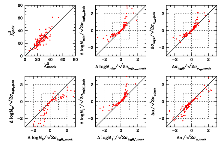
Figure 12: Comparison of best-fitting HOD parameters using mock and jackknife covariance matrices. Top left panel shows the comparison of $\chi^{2}$ for the best-fitting models using the two covariance matrices. The comparisons for the five HOD parameters are presented in other panels, as labelled. The red dots in each panel are the corresponding values for the $100$ mock catalogues. The dotted boxes indicate the ranges where the relative difference for each HOD parameter $\Delta p/\sqrt{2}\sigma_{p}=1$ or $2$.

In large-scale clustering analyses, it has become customary to use large sets of realistic mock catalogues, matching the observed clustering, to derive the error covariance matrix. However, when studying small-scale clustering and in particular when utilizing many subsamples with different clustering properties, jackknife resampling is a far more practical tool, and has been widely used for such studies (e.g. Zehavi et al. 2005, 2011; Guo et al. 2013).

Guo et al. (2013) demonstrated the accuracy of the jackknife errors for the projected 2PCF $w_{p}(r_{p})$ in comparison to the mock errors using a set of 100 mock catalogues from Manera et al. (2013). The ensemble average of jackknife errors shows good agreement with the mock errors (see Appendix B and specifically Figure 16 in Guo et al. 2013). For a given realization/sample, however, the jackknife covariance matrix still differs from the ensemble average and the mock covariance matrix. Here, we specifically study the accuracy of the jackknife covariance matrices when constraining the HOD parameters and show the jackknife covariance matrix from an individual sample works well in constraining the best-fitting HOD parameters.

We use the same set of 100 mock catalogues as in Guo et al. (2013). In each mock, we measure $w_{p}(r_{p})$ and the corresponding jackknife covariance matrix. We define the mock covariance matrix as the variance of $w_{p}(r_{p})$ among the $100$ mock catalogues. For each mock, we determine the best-fitting HOD parameters for the measured $w_{p}(r_{p})$ in this mock using the corresponding jackknife covariance matrix and compare to those parameters obtained from using the mock covariance matrix. To have a fair comparison of the best-fitting HOD parameters using the two covariance matrices, we define the relative difference for each parameter $p$ as $\Delta p/\sqrt{2}\sigma_{p}$, where $\Delta p\equiv p_{\rm mock}-p_{jack}$ is the difference between two best-fitting parameters and $\sigma_{p,{\rm mock}/{\rm jack}}$ is the marginalized 1$\sigma$ uncertainty on the parameter $p$ from modeling with either the mock or jackknife covariance matrix. The factor $\sqrt{2}$ comes from the fact that we are comparing the differences between two parameters, $p_{\rm mock}$ and $p_{\rm jack}$.

Figure 12 displays the comparison of $\chi^{2}$ for the best-fitting models using the two covariance matrices, as well as the relative differences for the five HOD parameters. The red dots in each panel are the corresponding values for the $100$ mock catalogues. The degree of freedom (dof) of the fitting is $14+1-5=10$. It is clear that the $\chi^{2}$ values of using the jackknife and mock covariance matrices are quite similar, implying that the two covariance matrices would produce similar goodness-of-fit for each mock. The large $\chi^{2}/\rm{dof}$ values could be caused by the fact that the mock catalogues do not fully describe the realistic galaxy clustering on small scales that can be captured by our HOD model (see e.g. White, Tinker, & McBride, 2014).

As shown in Figure 12, about $68$ per cent of the best-fitting HOD parameters derived from the two covariance matrices are within $1\sigma$ range of each other and about $92$ per cent lie within the $2\sigma$ errors. The parameter $\log M_{0}$, which determines the cut-off mass scale of the satellite galaxies and has more freedom in the models, is less constrained compared to other parameters. It is evident from the figure that the errors on the best-fitting HOD parameters derived from the two covariance matrices are also quite similar. We thus conclude that the jackknife covariance matrices will provide reasonably good estimates for best-fitting HOD parameters, compared to using the mock covariance matrices.

Appendix B Correlation Function Measurements

We present the measurements of the projected 2PCFs $w_{p}(r_{p})$ together with the diagonal errors used in this paper for the three luminosity-threshold samples and three colour samples in Table 5.

Table 5: Measurements of $w_{p}(r_{p})$ for the luminosity-threshold and finer colour samples

$r_{p}$	$M_{i}<-21.6$	$M_{i}<-21.8$	$M_{i}<-22.0$	‘green’	‘redseq’	‘reddest’
0.021	10029.85 (7420.09)	18138.15 (11600.27)	6986.76 (5854.06)	—	5079.46 (4095.05)	25888.67 (12384.27)
0.033	4744.70 (883.75)	6285.53 (1823.47)	12368.79 (4577.34)	—	3837.92 (2098.00)	12611.48 (3889.88)
0.052	2860.37 (359.76)	4659.69 (769.40)	5602.46 (1270.36)	1139.96 (782.25)	4282.92 (1368.53)	7798.45 (1785.71)
0.082	2732.31 (236.19)	3968.58 (420.99)	5185.31 (911.10)	2386.38 (849.47)	1772.59 (592.95)	3010.72 (722.82)
0.129	1560.89 (105.03)	1774.97 (171.64)	2225.19 (363.07)	496.75 (219.62)	893.92 (266.46)	3015.35 (414.65)
0.205	1025.62 (60.78)	1211.53 (108.33)	1792.21 (245.61)	562.86 (153.35)	820.90 (160.24)	1312.50 (200.97)
0.325	629.37 (30.65)	830.34 (54.38)	1009.84 (106.53)	370.83 (95.63)	591.31 (103.87)	723.29 (89.62)
0.515	363.88 (12.43)	441.23 (19.88)	620.87 (43.63)	189.24 (34.62)	333.02 (33.20)	456.22 (37.48)
0.815	195.87 (6.92)	233.84 (12.04)	333.99 (23.18)	149.75 (21.26)	178.01 (20.85)	226.14 (20.98)
1.292	128.80 (4.58)	154.92 (6.84)	199.46 (14.81)	97.87 (14.13)	124.07 (13.08)	136.52 (11.92)
2.048	92.67 (2.99)	106.21 (4.35)	124.62 (7.34)	70.30 (7.27)	87.86 (7.62)	112.16 (7.64)
3.246	67.65 (2.09)	80.95 (3.03)	101.29 (5.62)	55.93 (5.53)	53.45 (5.13)	71.87 (4.97)
5.145	48.11 (1.55)	55.99 (2.47)	65.71 (4.36)	39.00 (3.61)	45.81 (3.24)	56.05 (3.14)
8.155	32.13 (1.33)	36.70 (1.78)	44.27 (2.58)	28.13 (2.48)	29.49 (2.44)	37.54 (2.29)
12.92	19.56 (1.13)	22.27 (1.43)	24.94 (2.11)	14.88 (1.68)	18.57 (1.77)	24.36 (1.89)
20.48	10.59 (0.87)	12.80 (1.12)	15.17 (1.54)	7.99 (1.31)	10.89 (1.26)	11.16 (1.19)
32.46	3.73 (0.62)	4.58 (0.85)	5.82 (1.21)	2.86 (0.85)	3.85 (0.93)	4.75 (0.92)
51.45	1.24 (0.50)	2.03 (0.66)	2.64 (0.91)	1.38 (0.64)	1.09 (0.71)	0.95 (0.75)

The first column is the projected separation, $r_{p}$, in units of $\,h^{-1}{\rm{Mpc}}$. The subsequent columns present the projected 2PCFs, $w_{p}(r_{p})$, for different samples. The diagonal errors are given in parentheses.

References

- Ahn et al. (2014) Ahn C. P., et al., 2014, ApJS, 211, 17
- Akaike (1974) Akaike H., 1974, ITAC, 19, 716
- Anderson et al. (2012) Anderson L., et al., 2012, MNRAS, 427, 3435
- Anderson et al. (2013) Anderson L., et al., 2013, MNRAS submitted, arXiv:1312.4877
- Bahcall & Kulier (2013) Bahcall N. A., Kulier A., 2013, MNRAS in press, arXiv:1310.0022
- Benoist et al. (1996) Benoist C., Maurogordato S., da Costa L. N., Cappi A., Schaeffer R., 1996, ApJ, 472, 452
- Berlind & Weinberg (2002) Berlind A. A., Weinberg D. H., 2002, ApJ, 575, 587
- Berlind et al. (2003) Berlind A. A., et al., 2003, ApJ, 593, 1
- Beutler et al. (2013) Beutler F., et al., 2013, MNRAS, 429, 3604
- Blake, Collister, & Lahav (2008) Blake C., Collister A., Lahav O., 2008, MNRAS, 385, 1257
- Bolton et al. (2012) Bolton A. S., et al., 2012, AJ, 144, 144
- Brown et al. (2008) Brown M. J. I., et al., 2008, ApJ, 682, 937
- Budavári et al. (2003) Budavári T., et al., 2003, ApJ, 595, 59
- Bullock et al. (2001) Bullock J. S., Kolatt T. S., Sigad Y., Somerville R. S., Kravtsov A. V., Klypin A. A., Primack J. R., Dekel A., 2001, MNRAS, 321, 559
- Christodoulou et al. (2012) Christodoulou L., et al., 2012, MNRAS, 425, 1527
- Coil et al. (2006) Coil A. L., Newman J. A., Cooper M. C., Davis M., Faber S. M., Koo D. C., Willmer C. N. A., 2006, ApJ, 644, 671
- Coil et al. (2008) Coil A. L., et al., 2008, ApJ, 672, 153
- Coupon et al. (2012) Coupon J., et al., 2012, A&A, 542, A5
- Davis & Geller (1976) Davis M., Geller M. J., 1976, ApJ, 208, 13
- Davis et al. (1988) Davis M., Meiksin A., Strauss M. A., da Costa L. N., Yahil A., 1988, ApJ, 333, L9
- Dawson et al. (2013) Dawson K. S., et al., 2013, AJ, 145, 10
- Eisenstein & Hu (1998) Eisenstein D. J., Hu W., 1998, ApJ, 496, 605
- Eisenstein et al. (2011) Eisenstein D. J., et al., 2011, AJ, 142, 72
- Fry (1996) Fry J. N., 1996, ApJ, 461, L65
- Fukugita et al. (1996) Fukugita M., Ichikawa T., Gunn J. E., Doi M., Shimasaku K., Schneider D. P., 1996, AJ, 111, 1748
- Gao et al. (2005) Gao, L., Springel, V., & White, S. D. M. 2005, MNRAS, 363, L66
- Grillo (2012) Grillo C., 2012, ApJ, 747, L15
- Gunn et al. (1998) Gunn J. E., et al., 1998, AJ, 116, 3040
- Gunn et al. (2006) Gunn J. E., et al., 2006, AJ, 131, 2332
- Guo et al. (2014) Guo H., Li C., Jing Y. P., Börner G., 2014, ApJ, 780, 139
- Guo, Zehavi, & Zheng (2012) Guo H., Zehavi I., Zheng Z., 2012, ApJ, 756, 127
- Guo et al. (2013) Guo H., et al., 2013, ApJ, 767, 122 [G13]
- Guzzo et al. (1997) Guzzo L., Strauss M. A., Fisher K. B., Giovanelli R., Haynes M. P., 1997, ApJ, 489, 37
- Hamilton (1988) Hamilton A. J. S., 1988, ApJ, 331, L59
- Hartlap, Simon, & Schneider (2007) Hartlap J., Simon P., Schneider P., 2007, A&A, 464, 399
- Jannuzi & Dey (1999) Jannuzi B. T., Dey A., 1999, ASPC, 191, 111
- Jiang, Hogg, & Blanton (2012) Jiang T., Hogg D. W., Blanton M. R., 2012, ApJ, 759, 140
- Jing, Mo, & Boerner (1998) Jing Y. P., Mo H. J., Boerner G., 1998, ApJ, 494, 1
- Jing, Suto, & Mo (2007) Jing Y. P., Suto Y., Mo H. J., 2007, ApJ, 657, 664
- Kaiser (1987) Kaiser N., 1987, MNRAS, 227, 1
- Kravtsov et al. (2004) Kravtsov A. V., Berlind A. A., Wechsler R. H., Klypin A. A., Gottlöber S., Allgood B., Primack J. R., 2004, ApJ, 609, 35
- Kulkarni et al. (2007) Kulkarni G. V., Nichol R. C., Sheth R. K., Seo H.-J., Eisenstein D. J., Gray A., 2007, MNRAS, 378, 1196
- Landy & Szalay (1993) Landy S. D., Szalay A. S., 1993, ApJ, 412, 64
- Li et al. (2006) Li C., Kauffmann G., Jing Y. P., White S. D. M., Börner G., Cheng F. Z., 2006, MNRAS, 368, 21
- Loh et al. (2010) Loh Y.-S., et al., 2010, MNRAS, 407, 55
- Loveday et al. (1995) Loveday J., Maddox S. J., Efstathiou G., Peterson B. A., 1995, ApJ, 442, 457
- Madgwick et al. (2003) Madgwick D. S., et al., 2003, MNRAS, 344, 847
- Mandelbaum et al. (2006) Mandelbaum R., Seljak U., Kauffmann G., Hirata C. M., Brinkmann J., 2006, MNRAS, 368, 715
- Manera et al. (2013) Manera M., et al., 2013, MNRAS, 428, 1036
- Masjedi et al. (2006) Masjedi M., et al., 2006, ApJ, 644, 54
- Meneux et al. (2006) Meneux B., et al., 2006, A&A, 452, 387
- Meneux et al. (2008) Meneux B., et al., 2008, A&A, 478, 299
- Meneux et al. (2009) Meneux B., et al., 2009, A&A, 505, 463
- Miyatake et al. (2013) Miyatake H., et al., 2013, ApJ submitted, arXiv:1311.1480
- Navarro, Frenk, & White (1997) Navarro J. F., Frenk C. S., White S. D. M., 1997, ApJ, 490, 493
- Norberg et al. (2001) Norberg P., et al., 2001, MNRAS, 328, 64
- Norberg et al. (2002) Norberg P., et al., 2002, MNRAS, 332, 827
- Padmanabhan et al. (2009) Padmanabhan N., White M., Norberg P., Porciani C., 2009, MNRAS, 397, 1862
- Parejko et al. (2013) Parejko J. K., et al., 2013, MNRAS, 429, 98
- Peacock & Smith (2000) Peacock J. A., Smith R. E., 2000, MNRAS, 318, 1144
- Phleps et al. (2006) Phleps S., Peacock J. A., Meisenheimer K., Wolf C., 2006, A&A, 457, 145
- Ross & Brunner (2009) Ross A. J., Brunner R. J., 2009, MNRAS, 399, 878
- Ross et al. (2011) Ross A. J., et al., 2011, MNRAS, 417, 1350
- Ross, Percival, & Brunner (2010) Ross A. J., Percival W. J., Brunner R. J., 2010, MNRAS, 407, 420
- Schlegel, Finkbeiner, & Davis (1998) Schlegel D. J., Finkbeiner D. P., Davis M., 1998, ApJ, 500, 525
- Scoccimarro et al. (2001) Scoccimarro R., Sheth R. K., Hui L., Jain B., 2001, ApJ, 546, 20
- Seljak (2000) Seljak U., 2000, MNRAS, 318, 203
- Seo, Eisenstein, & Zehavi (2008) Seo H.-J., Eisenstein D. J., Zehavi I., 2008, ApJ, 681, 998
- Simon et al. (2009) Simon P., Hetterscheidt M., Wolf C., Meisenheimer K., Hildebrandt H., Schneider P., Schirmer M., Erben T., 2009, MNRAS, 398, 807
- Skibba & Sheth (2009) Skibba R. A., Sheth R. K., 2009, MNRAS, 392, 1080
- Skibba, Sheth, & Martino (2007) Skibba R. A., Sheth R. K., Martino M. C., 2007, MNRAS, 382, 1940
- Skibba et al. (2013) Skibba R. A., et al., 2013, arXiv, arXiv:1310.1093
- Smee et al. (2013) Smee S. A., et al., 2013, AJ, 146, 32
- Swanson et al. (2008) Swanson M. E. C., Tegmark M., Blanton M., Zehavi I., 2008, MNRAS, 385, 1635
- Tinker et al. (2005) Tinker J. L., Weinberg D. H., Zheng Z., Zehavi I., 2005, ApJ, 631, 41
- Tojeiro et al. (2012) Tojeiro R., et al., 2012, MNRAS, 424, 136
- van den Bosch et al. (2013) van den Bosch F. C., More S., Cacciato M., Mo H., Yang X., 2013, MNRAS, 430, 725
- Wake et al. (2008) Wake D. A., et al., 2008, MNRAS, 387, 1045
- Wake et al. (2011) Wake D. A., et al., 2011, ApJ, 728, 46
- Wang et al. (2007) Wang Y., Yang X., Mo H. J., van den Bosch F. C., 2007, ApJ, 664, 608
- Watson et al. (2012) Watson D. F., Berlind A. A., McBride C. K., Hogg D. W., Jiang T., 2012, ApJ, 749, 83
- Watson et al. (2010) Watson D. F., Berlind A. A., McBride C. K., Masjedi M., 2010, ApJ, 709, 115
- Wechsler et al. (2006) Wechsler, R. H., Zentner, A. R., Bullock, J. S., Kravtsov, A. V., & Allgood, B. 2006, ApJ, 652, 71
- Weinmann et al. (2006) Weinmann, S. M., van den Bosch, F. C., Yang, X., & Mo, H. J. 2006, MNRAS, 366, 2
- White et al. (2011) White M., et al., 2011, ApJ, 728, 126
- White, Tinker, & McBride (2014) White M., Tinker J. L., McBride C. K., 2014, MNRAS, 437, 2594
- White et al. (2007) White M., Zheng Z., Brown M. J. I., Dey A., Jannuzi B. T., 2007, ApJ, 655, L69
- Yang et al. (2005) Yang X., Mo H. J., Jing Y. P., van den Bosch F. C., 2005, MNRAS, 358, 217
- Yang, Mo, & van den Bosch (2003) Yang X., Mo H. J., van den Bosch F. C., 2003, MNRAS, 339, 1057
- York et al. (2000) York D. G., et al., 2000, AJ, 120, 1579
- Zehavi et al. (2002) Zehavi I., et al., 2002, ApJ, 571, 172
- Zehavi et al. (2005) Zehavi I., et al., 2005b, ApJ, 630, 1
- Zehavi et al. (2011) Zehavi I., et al., 2011, ApJ, 736, 59
- Zentner et al. (2005) Zentner A. R., Berlind A. A., Bullock J. S., Kravtsov A. V., Wechsler R. H., 2005, ApJ, 624, 505
- Zentner, Hearin, & van den Bosch (2013) Zentner A. R., Hearin A. P., van den Bosch F. C., 2013, MNRAS submitted, arXiv:1311.1818
- Zhao et al. (2009) Zhao D. H., Jing Y. P., Mo H. J., Börner G., 2009, ApJ, 707, 354
- Zheng (2004) Zheng Z., 2004, ApJ, 610, 61
- Zheng et al. (2005) Zheng Z., et al., 2005, ApJ, 633, 791
- Zheng, Coil, & Zehavi (2007) Zheng Z., Coil A. L., Zehavi I., 2007, ApJ, 667, 760
- Zheng et al. (2002) Zheng Z., Tinker J. L., Weinberg D. H., Berlind A. A., 2002, ApJ, 575, 617
- Zheng et al. (2009) Zheng Z., Zehavi I., Eisenstein D. J., Weinberg D. H., Jing Y. P., 2009, ApJ, 707, 554
- Zu et al. (2008) Zu Y., Zheng Z., Zhu G., Jing Y. P., 2008, ApJ, 686, 41