Geometric Proof of Strong Stable/Unstable Manifolds, with Application to the Restricted Three Body Problem

Abstract

We present a method for establishing strong stable/unstable manifolds of fixed points for maps and ODEs. The method is based on cone conditions, suitably formulated to allow for application in computer assisted proofs. In the case of ODEs, assumptions follow from estimates on the vector field, and it is not necessary to integrate the system. We apply our method to the restricted three body problem and show that for a given choice of the mass parameter, there exists a homoclinic orbit along matching strong stable/unstable manifolds of one of the libration points.

1 Introduction

In this paper we give a geometric method for establishing strong stable/unstable invariant manifolds of fixed points. The method is based on a graph transform type approach. Its assumptions are founded on suitably defined cone conditions, which can be verified using rigorous (interval arithmetic based), computer–assisted numerics.

Our approach is in a similar spirit to a number of previous results. The papers [17, 18] by Gidea and Zgliczyński introduced a topological tool referred to as “covering relations” or “correctly aligned windows”. The tool can be applied to obtain computer assisted proofs of symbolic dynamics in dynamical systems. A paper [30] by Zgliczyński extends the method by adding suitable cone conditions. With such additional assumptions one can establish existence of hyperbolic fixed points and their associated stable and unstable manifolds. The method has also been adapted by Zgliczyński, Simó and Capiński for proofs of normally hyperbolic invariant manifolds [6, 8, 9]. The above methods have been used and applied to a number of systems including the restricted three body problem [7, 11, 26, 27] rotating Hénon map [6, 9], driven logistic map [8], forced damped pendulum [29], and proofs of slow manifolds [19]. All these results rely on suitable definitions of covering relations and cone conditions. The result presented in this paper deals with fixed points, and is closely related to [30]. The main difference is that our result can be used to establish strong (un)stable manifolds, which could be submanifolds of the full (un)stable manifold. Our method can also be applied to saddle–center fixed points, which is not possible using [30], since it relies on hyperbolicity. Finally, our method does not rely on covering relations, which reduces the number of assumptions by half and simplifies their verification.

There are a number of alternative approaches for computer assisted proofs of invariant manifolds. These involve solving an appropriate fixed point equation in a functional setting. Amongst these methods it is notable to mention the work of Cabre, de la Llave, and Fontich [3, 4, 5]. Our approach is different. It follows from a topological argument performed in the state space of the system, instead of considering the problem in a functional setting. The assumptions of our theorem are simpler to verify, but at the cost of obtaining less accurate bounds on the manifold enclosure.

As an example of an application of our method we consider the planar circular restricted three body problem. We use the method to establish a rigorous enclosure of an unstable manifold of a libration fixed point of the problem. Using continuity based arguments, we also prove that the fixed point has a homoclinic orbit, for a suitably chosen parameter of the system. The example considered by us has first appeared in the work by Llibre, Martinez and Simó [21], where existence of such homoclinic connections has been demonstrated numerically. We validate their results using rigorous, interval based, computer assisted numerics.

To the best of our knowledge, our result is amongst the first computer assisted proofs of nontransversal homoclinic orbits for ODEs. The only other result known to us is the work of Szczelina and Zgliczyński [22], where a homoclinic orbit is proved for a two dimensional ODE. We note that the considered by us homoclinic connection in the restricted three body problem has not been proved up till this point. The only proof is the result of Llibre, Martinez and Simó [21], where an analytic argument is given for a sufficiently small mass parameter. Their method can not be applied though for a concrete given parameter, which is what we do in this paper.

Establishing of homoclinic connections between invariant objects can be used in the study of stability of a system. Combined with Melnikov type arguments, these can be used in proofs of Arnold diffusion [2] type dynamics. A broad selection of papers has used this approach, including the work of Delshams, Huguet, de la Llave, Seara or Treschev [13, 14, 15, 16, 24, 25] amongst many others. Such approach has also been applied in [10], in the setting of the planar elliptic restricted three body problem. It used the homoclinic connections from [21] for the Melnikov method. The result though was not fully rigorous, and relied on numerical computation of Melnikov integrals. The rigorous enclosure of the homoclinic orbit established in this paper can be a starting point for a rigorous validation of this computation. This would lead to a proof of Arnold diffusion type dynamics in the elliptic restricted three body problem. We plan to perform such validation in forthcoming work.

The paper is organized as follows. Section 2 contains preliminaries. In section 3 we state our results. In section 4 we present auxiliary results concerning cone conditions, which are then used in the proofs of our main results in section 5. Our results are written for maps. In section 6 we show how they can be applied for ODEs. Section 7 contains an application of our method, and contains a proof of existence of a homoclinic orbit to the libration point $L_{1}$ in the restricted three body problem. Sections 8, 9 and 10 contain closing remarks, acknowledgements and the appendix, respectively.

2 Preliminaries

2.1 Notations

Throughout the paper, all norms that appear are standard Euclidean norms. We use a notation $B(x,r)$ to denote a ball of radius $r$ centered at $x$. If we want to emphasize that a ball is in $\mathbb{R}^{k}$, then we add a subscript and write $B_{k}(x,r)$. We use a short hand notation $B_{k}=B_{k}(0,1)$ for a unit ball in $\mathbb{R}^{k}$ centered at zero. For a set $A\subset\mathbb{R}^{k}$ we use $\overline{A}$ to denote its closure and $\partial A$ for its boundary. For a point $p=\left(x,y\right)$ we use a notation $\pi_{x}p$ and $\pi_{y}p$ to denote projections onto $x$ and $y$ coordinates, respectively.

2.2 Computer assisted proofs

Most computations performed on a computer are burdened with error. Even very simple operations on real numbers (such as adding, multiplying or dividing) can result in round off errors. To make computer assisted computations fully rigorous, one can employ interval arithmetic, where instead of real numbers one deals with intervals. Any operation is made rigorous by appropriate rounding, which ensures an enclosure of the true result.

Interval arithmetic can also be used to treat basic functions (such as $\sin$, $\cos$ or exponent). It can be extended to perform linear algebra on interval vectors and interval matrices. One can thus design algorithms which give rigorous enclosures for multiplying matrices, inverting a matrix, computing eigenvectors or solving linear equations.

The interval arithmetic approach can also be extended to treat functions $f:\mathbb{R}^{n}\to\mathbb{R}^{m}$. One can implement algorithms which compute interval enclosures for images of the function $f$, for its derivative and for higher order derivatives.

The interval arithmetic approach can also be used for the integration of ODEs. One can implement interval arithmetic based integrators, which allow for the computation of enclosures of the images of points along of a flow of an ODE. One can extend such integrators to include the computation of high order derivatives of a time shift map along the flow, or even to compute high order derivatives for Poincaré maps [28].

All above mentioned tasks can be performed using a single C++ library “Computer Assisted Proofs in Dynamics” (CAPD for short). The package is freely available at:

http://capd.ii.uj.edu.pl

All the computer assisted proofs from this paper have been performed using CAPD.

2.3 Interval Newton Method

Let $X$ be a subset of $\mathbb{R}^{n}$. We shall denote by $[X]$ an interval enclosure of the set $X$, that is, a set

$$[X]=\Pi_{i=1}^{n}[a_{i},b_{i}]\subset\mathbb{R}^{n},$$

such that

$$X\subset[X].$$

Let $f:\mathbb{R}^{n}\to\mathbb{R}^{n}$ be a $C^{1}$ function and $U\subset\mathbb{R}^{n}$. We shall denote by $[Df(U)]$ the interval enclosure of a Jacobian matrix on the set $U$. This means that $[Df(U)]$ is an interval matrix defined as

$$[Df(U)]=\left\{A\in\mathbb{R}^{n\times n}|A_{ij}\in\left[\inf_{x\in U}\frac{df_{i}}{dx_{j}}(x),\sup_{x\in U}\frac{df_{i}}{dx_{j}}(x)\right]\text{ for all }i,j=1,\ldots,n\text{ }\right\}.$$

Theorem 1

[1] (Interval Newton method) Let $f:\mathbb{R}^{n}\rightarrow\mathbb{R}^{n}$ be a $C^{1}$ function and $X=\Pi_{i=1}^{n}[a_{i},b_{i}]$ with $a_{i}<b_{i}$. If $[Df(X)]$ is invertible and there exists an $x_{0}$ in $X$ such that

$$N(x_{0},X):=x_{0}-\left[Df(X)\right]^{-1}f(x_{0})\subset X,$$

then there exists a unique point $x^{\ast}\in X$ such that $f(x^{\ast})=0.$

2.4 Restricted three body problem

The problem is defined as follows: two main bodies rotate in the plane about their common center of mass on circular orbits under mutual gravitational influence. A third body moves in the same plane of motion as the two main bodies, attracted by their gravitation, but not influencing their motion. The problem is to describe the motion of the third body.

Usually, the two rotating bodies are referred to as the primaries. The third body can be regarded as a satellite or a spaceship of negligible mass.

We use a rotating system of coordinates centred at the center of mass. The plane $X,Y$ rotates with the primaries. The primaries are on the $X$ axis, the $Y$ axis is perpendicular to the $X$ axis and contained in the plane of rotation.

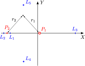
Figure 1: Rotating system of coordinates with origin at the center of mass. The sun has the mass $1-\mu$ and is fixed at $P_{1}=(\mu,0)$. The planet has the mass $\mu$ is fixed at $P_{2}=(\mu-1,0)$. The third massless particle moves in the $XY$ plane.

We rescale the masses $\mu_{1}$ and $\mu_{2}$ of the primaries so that they satisfy the relation $\mu_{1}+\mu_{2}=1$. After such rescaling the distance between the primaries is $1$. (See Szebehelly [23], section 1.5). We refer to the larger of the two primaries as the “sun” and to the smaller as the “planet”. We use a convention in which in the rotating coordinates the sun is located to the right of the origin at $P_{1}=(\mu,0)$, and the planet is located to the left at $P_{2}=(\mu-1,0)$.

The equations of motion of the third body are

$$\ddot{X}-2\dot{Y} =\Omega_{X},$$

$$\ddot{Y}+2\dot{X} =\Omega_{Y},$$

where

$$\Omega=\frac{1}{2}(X^{2}+Y^{2})+\frac{1-\mu}{r_{1}}+\frac{\mu}{r_{2}},$$

and $r_{1},r_{2}$ denote the distances from the third body to the larger and the smaller primary, respectively (see Figure 1)

$$r_{1}^{2} =(X-\mu)^{2}+Y^{2},$$

$$r_{2}^{2} =(X-\mu+1)^{2}+Y^{2}.$$

These equations have an integral of motion [23] called the Jacobi integral

$$C=2\Omega-(\dot{X}^{2}+\dot{Y}^{2}).$$

The equations of motion take Hamiltonian form if we consider positions $X$, $Y$ and momenta $P_{X}=\dot{X}-Y$, $P_{Y}=\dot{Y}+X$. The Hamiltonian is

$$H=\frac{1}{2}(P_{X}^{2}+P_{Y}^{2})+YP_{X}-XP_{Y}-\frac{1-\mu}{r_{1}}-\frac{\mu}{r_{2}},$$ (2)

with the vector field given by

$$F =J\nabla H,$$

$$J =\left(\begin{array}[c]{cc}0&\mathrm{id}\\ -\mathrm{id}&0\end{array}\right),\quad\mathrm{id}=\left(\begin{array}[c]{cc}1&0\\ 0&1\end{array}\right).$$

The Hamiltonian and the Jacobi integral are simply related by $H=-\frac{C}{2}$.

Due to the Hamiltonian integral, the dimensionality of the space can be reduced by one. Trajectories of the system stay on the energy surface $M$ given by $H(X,Y,P_{X},P_{Y})=h=$constant. Equivalently, $M$ is the level surface

$$M\equiv\{C(X,Y,\dot{X},\dot{Y})=c=-2h\}$$ (3)

of the Jacobi integral.

The problem has a reversing symmetry defined by

$$S(X,Y,P_{X},P_{Y})=\left(X,-Y,-P_{X},P_{Y}\right).$$ (4)

Using a notation $\mathbf{x}=\left(X,-Y,-P_{X},P_{Y}\right)$ for the coordinates, and $\phi_{t}(\mathbf{x})$ for the flow of the vector field

$$\mathbf{\dot{x}}=J\nabla H(\mathbf{x}),$$

the system has the property

$$S(\phi_{t}(\mathbf{x}))=\phi_{-t}(S(\mathbf{x})).$$ (5)

The problem has five equilibrium points (see [23]). Three of them, denoted $L_{1},L_{2}$ and $L_{3}$, lie on the $X$-axis and are usually called the ‘collinear’ equilibrium points (see Figure 1). Notice that we denote $L_{1}$ the interior collinear point, located between the primaries.

The Jacobian of the vector field at $L_{1}$ has two real and two purely imaginary eigenvalues. It possesses a one dimensional unstable manifold. By (5), the one dimensional stable manifold is $S$-symmetric to the unstable manifold.

3 Statement of main results

Our paper contains two results. The first is a method for establishing strong invariant manifolds for fixed points. The method is based on cone conditions, and is tailor made for rigorous (interval based) computer assisted implementation. The second result is an application of the method to prove a homoclinic connection of a libration fixed point in the restricted three body problem.

3.1 Establishing strong invariant manifolds

Let $N=\overline{B}_{u}\times\overline{B}_{s}$ and

$$f:N\rightarrow\mathbb{R}^{u}\times\mathbb{R}^{s}$$

be a $C^{1}$ function. We assume that there exists a fixed point for $f$ in the interior of $N$. For simplicity we assume that the fixed point is at zero. This assumption can easily be relaxed (see Remark 13).

Our method can be applied to establish strong stable and strong unstable manifolds defined as follows:

Definition 2

Let $U$ be a neighborhood of zero and let $\lambda<1$. A set $W_{\lambda,U}^{s}\subset U$ consisting of all points $p\in U$ satisfying:

1. $f^{n}(p)\in U$ for any $n\in\mathbb{N}$;

2. there exists a constant $C>0$ (which can depend on $p$), such that for all $n\geq 0$

   $$\left\|f^{n}(p)\right\|\leq C\lambda^{n};$$ (6)

is called a strong stable manifold, with contraction rate $\lambda$, in $U$.

Definition 3

Let $U\subset\mathbb{R}^{u}\times\mathbb{R}^{s}$ be a set and let $p\in U$. We say that a sequence $(p_{0},p_{-1},p_{-2},\ldots)$ is a backward trajectory of $p$ in $U$ if $p_{0}=p$ and for any $i<0$, $p_{i}\in U$ and $p_{i+1}=f(p_{i})$.

Definition 4

Let $U$ be a neighborhood of zero and let $\lambda>1$. A set $W_{\lambda,U}^{u}\subset U$ consisting of all points $p\in U$ satisfying:

1. there exists a backward trajectory $(p_{0},p_{-1},p_{-2},\ldots)$ of $p$ in $U$;

2. for any backward trajectory $(p_{0},p_{-1},p_{-2},\ldots)$ of $p$ in $U$ there exists a constant $C>0$ (which can depend on the backward trajectory), such that for all $n\leq 0$

   $$\left\|p_{n}\right\|\leq C\lambda^{n};$$ (7)

is called a strong unstable manifold, with expansion rate $\lambda$, in $U$.

Example 5

Let $f_{1}(x,y)=(\frac{1}{2}x,\frac{1}{3}y)$. The stable manifold with contraction rate $\frac{1}{2}$ in $\mathbb{R}^{2}$ is equal to $\mathbb{R}^{2}$ and the stable manifold with contraction rate $\frac{1}{3}$ in $\mathbb{R}^{2}$ is $\left\{0\right\}\times\mathbb{R}$. Similarly, for $f_{2}(x,y)=(2x,3y)$ the unstable manifold with expansion rate $2$ in $\mathbb{R}^{2}$ is $\mathbb{R}^{2}$ and the unstable manifold with expansion rate $3$ in $\mathbb{R}^{2}$ is $\left\{0\right\}\times\mathbb{R}$.

Let $\alpha_{h},\alpha_{v}\in(0,1)$ and let

$$Q_{h},Q_{v}:\mathbb{R}^{u}\times\mathbb{R}^{s}\rightarrow\mathbb{R}$$

be defined as

$$Q_{h}(x,y) =\alpha_{h}\left\|x\right\|^{2}-\left\|y\right\|^{2}$$ (8)

$$Q_{v}(x,y) =\left\|x\right\|^{2}-\alpha_{v}\left\|y\right\|^{2}.$$ (9)

Definition 6

Let $\alpha,\beta,m>0$ and let $Q(x,y)=\alpha\left\|x\right\|^{2}-\beta\left\|y\right\|^{2}.$ We say that $f$ satisfies cone conditions for $(Q,m)$ in $N$ if for any $p_{1}\neq p_{2},$ $p_{1},p_{2}\in N,$ holds

$$Q(f(p_{1})-f(p_{2}))>mQ(p_{1}-p_{2}).$$

The following theorems are the main results of our paper.

Theorem 7

Assume that $m_{v}>m_{h}>0$ and $m_{v}>1$. Let $r^{u}=\sqrt{1-\alpha_{v}}$ and $U=\overline{B}_{u}(0,r^{u})\times\overline{B}_{s}$. If $f$ satisfies cone conditions for $(Q_{h},m_{h})$ and $(Q_{v},m_{v})$ in $N,$ then there exists a function $w^{u}:\overline{B}_{u}(0,r^{u})\rightarrow\overline{B}_{s},$ such that

$$W_{\sqrt{m_{v}},N}^{u}\cap U=\left\{(x,w^{u}(x))|x\in\overline{B}_{u}(0,r^{u})\right\}.$$

Moreover, $w^{u}$ is Lipschitz with a constant $L_{u}=\sqrt{\alpha_{h}}$.

Theorem 8

Assume that $m_{v}>m_{h}>0$ and $m_{h}<1.$ Let $r^{s}=\sqrt{1-\alpha_{h}}$ and $U=\overline{B}_{u}\times\overline{B}_{s}(0,r^{s}).$ If $f$ satisfies cone conditions for $(Q_{h},m_{h})$ and $(Q_{v},m_{v})$ in $N,$ then there exists a function $w^{s}:\overline{B}_{s}(0,r^{s})\rightarrow B_{u},$ such that

$$W_{\sqrt{m_{h}},N}^{s}\cap U=\left\{(w^{s}(y),y)|y\in\overline{B}_{s}(0,r^{s})\right\}.$$

Moreover, $w^{s}$ is Lipschitz with a constant $L_{s}=\sqrt{\alpha_{v}}.$

The proofs of Theorems 7, 8 are given in Section 5.

Remark 9

Let us say that the fixed point has a stable manifold. Theorem 8 can be used to establish a lower dimensional manifold (which is a sub manifold of the full stable manifold), that is associated with some prescribed contraction rate. For instance, $f_{1}$ from Example 5 has such a lower dimensional stable manifold that is associated with contraction rate $\lambda=\frac{1}{3}$.

Similarly, Theorem 7 can be used to establish lower dimensional submanifolds of an unstable manifold, that are associated with prescribed expansion rates. The $f_{2}$ from Example 5 has such a lower dimensional unstable manifold that is associated with expansion rate $\lambda=3$.

Theorems 7, 8 are formulated for maps. In Section 6 we show mirror results for flows (see Theorems 32, 33). We emphasize that these results do not require rigorous integration, but follows directly from appropriate bounds on the vector field.

Let us point out that assumptions of Theorems 7, 8 can easily be verified using the following lemma.

Lemma 10

Let $\alpha,\beta,m>0$ and let $Q(x,y)=\alpha\left\|x\right\|^{2}-\beta\left\|y\right\|^{2}.$ Assume that for any $B\in\left[Df(N)\right],$ the quadratic form

$$V(q)=Q(Bq)-mQ(q)$$

is positive definite, then $f$ satisfies cone conditions for $(Q,m)$ in $N$.

Proof. The proof is given in Appendix 10.1.   

There are a number of algorithms that can be used to verify if a matrix is positive definite. This can also be done using interval arithmetic.

Let us finish the section with simple examples, which provide some intuition for the results.

Example 11

Let $a,b\in\mathbb{R}$, $a>b>0$, and let $f:N\rightarrow\mathbb{R}^{2}$ be a linear map

$$f(x,y)=\left(ax,by\right),$$

then $f$ satisfies cone conditions for $(Q_{h},m_{h})$ and $(Q_{v},m_{v})$ for any $m_{h},m_{v}\in\left(b^{2},a^{2}\right)$. Let us note that we do not need to assume that $a>1$ or that $b<1$. Moreover, $f_{\varepsilon}=f+\varepsilon g$ satisfies cone conditions, provided that $g$ is differentiable and $\varepsilon$ is small enough.

Example 12

Let $a,b\in\mathbb{R}$, $a>1>b>0$ and let $R:\mathbb{R}^{2}\ni\theta\rightarrow R(\theta)\in\mathbb{R}^{2}$ be a rotation. Consider $f:\mathbb{R}^{4}\rightarrow\mathbb{R}^{4},$ of the form

$$f\left(\xi,\theta,\eta\right)=\left(a\xi,R(\theta),b\eta\right).$$

For coordinates $x_{1},y_{1}$ chosen as

$$x_{1}=\xi,\qquad y_{1}=(\theta,\eta),$$

assumptions of Theorem 7 are satisfied for any $\alpha_{h},\alpha_{v}\in\left(0,1\right)$ and any $m_{h},m_{v}\in(1,a^{2})$ satisfying $m_{v}>m_{h}$.

On the other hand, for coordinates $x_{2},y_{2}$ chosen as

$$x_{2}=\left(\xi,\theta\right),\qquad y_{2}=\eta,$$

assumptions of Theorem 8 are satisfied for any $\alpha_{h},\alpha_{v}\in\left(0,1\right)$ and any $m_{h},m_{v}\in(b^{2},1)$ satisfying $m_{v}>m_{h}$

We thus see that we can apply Theorems 7 and 8 by swapping the roles of some of the coordinates.

The assumptions still hold for $f_{\varepsilon}=f+\varepsilon g,$ provided that $g$ is differentiable and $\varepsilon$ is small enough.

We conclude this section with a remark that the fixed point does not need to be centered at zero in order to apply our method.

Remark 13

The proofs of Theorems 7 and 8 are conducted under the assumption that the fixed point is at zero. In many applications though it can be difficult to establish the fixed point analytically. In computer assisted proofs the enclosure of a fixed point can be obtained using the interval Newton theorem (Theorem 1). Assuming that we know that the fixed point is contained in a set $B\subset\mathbb{R}^{u+s},$ it is sufficient to verify cone conditions on a set $N^{\prime}=N+B$.

3.2 Establishing existence of homoclinic orbits in the restricted three body problem

In the work by Llibre, Martinez and Simó [21] it is shown that for suitably chosen family of parameters $\mu\in\{\mu_{k}^{\ast}\}_{k=2}^{\infty}$, $\mu_{k+1}^{\ast}<\mu_{k}^{\ast},$ the unstable and stable manifolds of $L_{1}^{\mu_{k}^{\ast}}$ coincide, leading to a homoclinic orbit. The paper [21] contains numerical evidence of such homoclinic orbits for the first number of the larger of these parameters $\mu_{k}^{\ast}$, and gives an analytic proof for sufficiently small $\mu_{k}^{\ast}$.

The aim of this section is to show that using our method it is possible to obtain rigorous enclosures of the stable and unstable manifolds, and to validate the existence of homoclinic orbits for the large values of $\mu_{k}^{\ast}$. We focus on the largest of the parameters

$$\mu_{2}^{\ast}\approx 0.004253863522$$

and prove that

$$\mu_{2}^{\ast}\in 0.004253863522+10^{-10}\left[-1,1\right].$$

The established homoclinic connection is depicted in Figure 2.

Remark 14

Our estimate on the parameter for which we have a homoclinic orbit to $L_{1}^{\mu_{2}^{\ast}}$ is very tight. This is thanks to the fact that our method for establishing invariant manifolds produces very tight rigorous bounds. This demonstrates that it is a tool that can successfully be applied for nontrivial problems.

Remark 15

Our paper focuses on $\mu_{2}^{\ast}$ since it is the largest parameter, hence furthest away from the analytic proof of [21]. Using our method one can obtain a proof also for other parameters. As the parameters become smaller though, the proof becomes more challenging numerically.

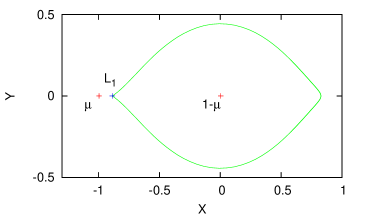
Figure 2: Homoclinic orbit in green, the masses in red, and the fixed point $L_{1}$ in blue.

4 Cones and horizontal discs

In this section we give some auxiliary results, which are then used in the proofs of Theorems 7, 8 in section 5.

We start with some simple facts which follow straight from (8–9). We formulate this as a remark, and give the proof in the appendix.

Remark 16

1. If $\left\|x\right\|\leq 1$ and $Q_{h}\left(x,y\right)\geq\alpha_{h}-1,$ then $\left\|y\right\|\leq 1.$

2. If $\left\|y\right\|\leq 1$ and $Q_{v}\left(x,y\right)\leq 1-\alpha_{v}$ then $\left\|x\right\|\leq 1$.

3. If $Q_{h}\left(x,y\right)\geq\alpha_{h}-1$ and $Q_{v}\left(x,y\right)\leq 1-\alpha_{v}$ then $(x,y)\in N$.

4. If $\left\|y\right\|\leq a$ then $Q_{h}\left(x,y\right)\geq-a^{2}$.

Proof. The proof is given in Appendix 10.2.   

We now give two technical lemmas.

Lemma 17

Assume that $(q_{0},q_{-1},q_{-2},\ldots)$ is a backward trajectory in $\{Q_{h}\geq 0\}\cap N$. If $f$ satisfies cone conditions for $(Q_{v},m_{v}),$ then for $C=\sqrt{2\left(1-\alpha_{v}\alpha_{h}\right)^{-1}}$ and any $k\leq 0$

$$\left\|q_{k}\right\|\leq C\left(\sqrt{m_{v}}\right)^{k}.$$

Proof. The proof is given in Appendix 10.3.   

Lemma 18

Assume that for a $q_{0}\in N$, for all $k\geq 0,$ $f^{k}(q_{0})\in\{Q_{v}\leq 0\}\cap N.$ If $f$ satisfies cone conditions for $\left(Q_{h},m_{h}\right),$ then for $C=\sqrt{2\left(1-\alpha_{v}\alpha_{h}\right)^{-1}}$ and any $k\geq 0$

$$\left\|f^{k}(q_{0})\right\|\leq C\left(\sqrt{m_{h}}\right)^{k}.$$

Proof. The proof is given in Appendix 10.4.   

We now introduce a notion of a horizontal disc. Horizontal discs will be the building blocks in our construction of the invariant manifolds.

Definition 19

Let $Q(x,y)=\alpha\left\|x\right\|^{2}-\beta\left\|y\right\|^{2}$ for $\alpha,\beta>0$. Let $h:\overline{B}_{u}\rightarrow\mathbb{R}^{u+s}$ be a continuous mapping. We say that $h$ is a $Q$-horizontal disc if

$$Q(h(x_{1})-h(x_{2})) >0\text{ for any }x_{1}\neq x_{2},$$ (10)

$$\pi_{x}h(0) =0.$$ (11)

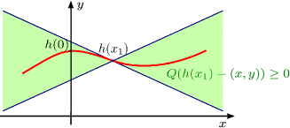
Figure 3: A $Q$-horizontal disc $h$ in red. For any point $x_{1}\in\overline{B}_{u}$ the disc $h$ lies within the interior of a cone attached at $h(x_{1})$.

Definition 20

We say that a $Q$-horizontal disc is in $N$ if $h(B_{u})\subset N.$

Definition 21

Let $c>0$. We say that a $Q$-horizontal disc has radius $c$ if

$$Q(h\left(\partial B_{u}\right))=c,$$ (12)

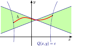
Figure 4: A $Q$-horizontal disc $h$ with radius $c$ (in red). The image $\partial B_{u}$ is contained in the set $\left\{Q=c\right\}$.

Let $Q(x,y)=\alpha\left\|x\right\|^{2}-\beta\left\|y\right\|^{2}$ for $\alpha,\beta>0$. The following lemmas are consequences of Definition 19.

Lemma 22

If $h$ is a $Q$-horizontal disc, then $\pi_{x}\circ h$ is bijective onto its image.

Proof. Take any $x_{1},x_{2}\in\overline{B}_{u}$ and suppose that $\pi_{x}(h(x_{1}))=\pi_{x}(h(x_{2}))$. Then

$$Q(h(x_{1})-h(x_{2}))=-\beta||\pi_{y}(h(x_{1}))-\pi_{y}(h(x_{2}))||^{2}\leq 0$$

The condition (10) implies that $x_{1}=x_{2}$. It means that $\pi_{x}\circ h$ is injective, and as a consequence it is bijective onto its image.   

Lemma 23

If $h$ is a $Q$-horizontal disc of radius $c$, then for any $x^{\ast}\in\overline{B}_{u}\left(0,\sqrt{\frac{c}{\alpha}}\right),$ there exists a unique $x$ such that $\pi_{x}h(x)=x^{\ast}$.

Proof. By definition, $h$ is continuous. By Lemma 22, $\pi_{x}h:\overline{B}_{u}\rightarrow\mathbb{R}^{u}$ is injective. This means that $\pi_{x}h\left(B_{u}\right)$ is homeomorphic to a ball in $\mathbb{R}^{u}$.

For any $x\in\partial B_{u}$

$$c=Q(h(x))=\alpha\left\|\pi_{x}h(x)\right\|^{2}-\beta\left\|\pi_{y}h(x)\right\|^{2}\leq\alpha\left\|\pi_{x}h(x)\right\|^{2},$$

hence $\left\|\pi_{x}h(x)\right\|\geq\sqrt{\frac{c}{\alpha}}.$ This means that $\partial\left[\pi_{x}h\left(B_{u}\right)\right]\cap B_{u}\left(0,\sqrt{\frac{c}{\alpha}}\right)=\emptyset,$ hence either

$$\pi_{x}h\left(B_{u}\right)\cap B_{u}\left(0,\sqrt{\frac{c}{\alpha}}\right)=\emptyset,$$

or

$$B_{u}\left(0,\sqrt{\frac{c}{\alpha}}\right)\subset\pi_{x}h\left(B_{u}\right).$$ (13)

Since $\pi_{x}h(0)=0\in B_{u}\left(0,\sqrt{\frac{c}{\alpha}}\right),$ we see that (13) must be the case. From (13), by continuity of $h$,

$$\overline{B}_{u}\left(0,\sqrt{\frac{c}{\alpha}}\right)\subset\pi_{x}h\left(\overline{B}_{u}\right).$$

We have thus shown that for any $x^{\ast}$ there exists an $x$ such that $\pi_{x}h(x)=x^{\ast}$. Such point needs to be unique since for $x_{1}\neq x_{2}$

$$0 <\frac{1}{\alpha}Q\left(h(x_{1})-h(x_{2})\right)$$

$$=\left\|\pi_{x}h(x_{1})-\pi_{x}h(x_{2})\right\|^{2}-\frac{\beta}{\alpha}\left\|\pi_{y}h(x_{1})-\pi_{y}h(x_{2})\right\|^{2}$$

$$\leq\left\|\pi_{x}h(x_{1})-\pi_{x}h(x_{2})\right\|^{2}.$$

 

Let $Q(x,y)=\alpha\left\|x\right\|^{2}-\beta\left\|y\right\|^{2}$ for $\alpha,\beta>0$, and let $c^{\ast}>0$. In the following arguments we shall use the function $\phi:\mathbb{R}^{u}\times\mathbb{R}^{s}\rightarrow\mathbb{R}^{u}\times\mathbb{R}^{s}$

$$\phi(u,s)=\left\{\begin{array}[c]{ll}\left(u\sqrt{\frac{1}{\alpha}\left(c^{\ast}+\beta\left\|s\right\|^{2}\right)},s\right)&\qquad\text{if }\left\|u\right\|\leq 1,\\ \left(u\left[\frac{1}{\left\|u\right\|}\left(\sqrt{\frac{1}{\alpha}\left(c^{\ast}+\beta\left\|s\right\|^{2}\right)}-1\right)+1\right],s\right)&\qquad\text{if }\left\|u\right\|>1,\end{array}\right.$$ (14)

which will be used as a suitable change of coordinates. (Note that $\phi$ is continuous.) The choice of $\phi$ is motivated by the fact that $\{\phi(u,s):\left\|u\right\|\leq 1\}=\left\{Q\leq c^{\ast}\right\}$. Thus, we can say that $\phi$ “straightens out” $\left\{Q\leq c^{\ast}\right\}$ (see Figure 5). We now give a technical lemma.

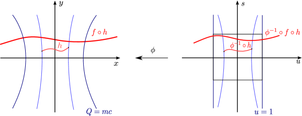
Figure 5: The change of coordinates $\phi$ applied to a $Q$-horizontal disc $h$ and to $f\circ h$.

Lemma 24

If $s_{1},s_{2}\in\mathbb{R}^{s}$ and $u\in\mathbb{R}^{u}$ then

$$Q\left(\phi(u,s_{1})-\phi(u,s_{2})\right)\leq 0.$$

Proof. For $a,b>0$

$$x\rightarrow\sqrt{b+a\left\|x\right\|^{2}}$$

is Lipschitz with constant $\sqrt{a},$ thus

$$\left\|\pi_{x}\left(\phi(u,s_{1})-\phi(u,s_{2})\right)\right\| \leq\sqrt{\frac{\beta}{\alpha}}\left\|s_{1}-s_{2}\right\|,$$ (15)

$$\left\|\pi_{y}\left(\phi(u,s_{1})-\phi(u,s_{2})\right)\right\| =\left\|s_{1}-s_{2}\right\|.$$

This gives that for any $s_{1},s_{2}$

$$Q\left(\phi(u,s_{1})-\phi(u,s_{2})\right)\leq\alpha\left(\sqrt{\frac{\beta}{\alpha}}\left\|s_{1}-s_{2}\right\|\right)^{2}-\beta\left\|s_{1}-s_{2}\right\|^{2}=0,$$ (16)

as required.   

The following lemma is a key result that will be used in our construction of the manifolds.

Lemma 25

Let $Q(x,y)=\alpha\left\|x\right\|^{2}-\beta\left\|y\right\|^{2}$ for $\alpha,\beta>0$. Let $h:\overline{B}_{u}\rightarrow N$ be a $Q$-horizontal disc in $N$ of radius $c>0.$ Let $m>0.$ If $f$ satisfies cone conditions for $(Q,m),$ then for any $c^{\ast}\in(0,mc]$ there exists a $Q$-horizontal disc $h^{\ast}:\overline{B}_{u}\rightarrow\mathbb{R}^{u+s}$ of radius $c^{\ast}$, such that

$$h^{\ast}(\overline{B}_{u})=f\circ h(\overline{B}_{u})\cap\{Q\leq c^{\ast}\},$$ (17)

and

$$\pi_{u}\phi^{-1}(h^{\ast}(u))=u.$$ (18)

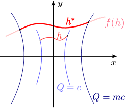
Figure 6: $Q$-horizontal disc $h^{*}$ with radius $c^{*}=mc$ obtained as an intersection of an image under $f$ of a $Q$-horizontal disc $h$ of radius $c$, and the set $\{Q\leq c^{*}\}$ (see Lemma 25).

Proof. Let $h_{\lambda}(x):=(\pi_{x}h(x),\lambda\pi_{y}h(x))$ and let us define the function

$$H:[0,1]\times\overline{B}_{u}\rightarrow[0,1]\times\mathbb{R}^{u},$$

$$H(\lambda,x)=\left(\lambda,\pi_{u}\phi^{-1}\left(f(h_{\lambda}(x))\right)\right).$$

We will show that $H$ is an open map. Observe that $h_{\lambda}$ are $Q$-horizontal discs in $N$. Let $x_{1},x_{2}\in\overline{B}_{u}$ and $x_{1}\neq x_{2}$. By the fact that $f$ satisfies cone conditions, $Q\left(f(h_{\lambda}(x_{1}))-f(h_{\lambda}(x_{2}))\right)>0$, and by Lemma 24 we can not have $\pi_{u}\phi^{-1}(f(h_{\lambda}(x_{1})))=\pi_{u}\phi^{-1}(f(h_{\lambda}(x_{1}))).$ Hence $H$ is injective. By definition, $H$ is also continuous, thus it is an open map.

We consider the set $[0,1]\times\mathbb{R}^{u}$, with topology induced from $\mathbb{R}\times\mathbb{R}^{u}$. Let $A=[0,1]\times B_{u}$. Note that $A$ is open in $[0,1]\times\mathbb{R}^{u}$, that $clA=[0,1]\times\overline{B}_{u}$ and $\partial A=\left[0,1\right]\times\partial B_{u}$. Since $H$ is an open map, $H(A)\cap clA$ is open in $clA.$ We will show that $H(A)\cap clA$ is also closed in $clA$.

Take any $x\in\partial B_{u}$. Since $Q(h_{\lambda}(x))\geq Q(h(x))=c$, by the fact that $f$ satisfies cone conditions for $(Q,m)$

$$Q(f(h_{\lambda}(x)))>mQ(h_{\lambda}(x))\geq mc\geq c^{\ast}.$$

Hence $\pi_{u}\phi^{-1}\left(f(h_{\lambda}(\partial B_{u}))\right)\cap\overline{B}_{u}=\emptyset,$ which means that for all $\lambda\in[0,1]$

$$H\left(\partial A\right)\cap\mathrm{cl}A=H(\left[0,1\right]\times\partial B_{u})\cap\mathrm{cl}A=\emptyset.$$ (19)

We thus see that $H(A)\cap\mathrm{cl}A$ is closed in $\mathrm{cl}A$.

Since $H(A)\cap\mathrm{cl}A$ is both open and closed in $\mathrm{cl}A$, we either have

$$H(A)\cap\mathrm{cl}A=\mathrm{cl}A,$$

or

$$H(A)\cap\mathrm{cl}A=\emptyset.$$ (20)

Since $h_{\lambda=0}(0)=0,$ $f\left(0\right)=0\$and $\phi^{-1}(0)=0$,

$$H\left(0,0\right)=\left(0,\pi_{u}\phi^{-1}\left(f(h_{\lambda=0}(0))\right)\right)=\left(0,0\right)\in A.$$

We see that we can not have (20), hence $\mathrm{cl}A\subset H(A)$. This in particular implies that $\left\{1\right\}\times\overline{B}_{u}\subset H(\{1\}\times B_{u})$, hence

$$\overline{B}_{u}\subset\pi_{u}\phi^{-1}\left(f(h(\overline{B}_{u}))\right).$$ (21)

From (21) we see that for any $u\in\overline{B}_{u}$ there exists an $x=x(u)\in B_{u},$ such that

$$u=\pi_{u}\phi^{-1}\left(f(h(x(u)))\right).$$ (22)

We now define

$$h^{\ast}(u)=f(h(x(u))).$$ (23)

Note that from (22) and (23) follows (18).

For $h^{\ast}$ to be well defined we need to show that the choice of $x(u)$ is unique. Assume that for $x_{1}\neq x_{2}$ we have

$$\phi^{-1}\left(f(h(x_{1}))\right) =\left(u,s_{1}\right)$$

$$\phi^{-1}\left(f(h(x_{2}))\right) =\left(u,s_{2}\right)$$

with $s_{1}\neq s_{2}$. From Lemma 24 we know that

$$Q\left(\phi(u,s_{1})-\phi(u,s_{2})\right)\leq 0.$$

On the other hand,

$$Q\left(\phi(u,s_{1})-\phi(u,s_{2})\right)=Q\left(f(h(x_{1}))-f(h(x_{2}))\right)>mQ\left(h(x_{1})-h(x_{2})\right)>0.$$ (24)

We obtain a contradiction, hence we must have $s_{1}=s_{2}.$ This shows that $h^{\ast}$ is well defined.

We need to show that $h^{\ast}$ is a $Q$-horizontal disc of radius $c^{\ast}$. We first show (10). Observe that (22) implies that $x(u_{1})\neq x(u_{2})$ for any $u_{1}\neq u_{2}$. From (23) and by the fact that $f$ satisfies cone conditions for $(Q,m)$

$$Q(h^{\ast}(x_{1})-h^{\ast}(x_{2})) =Q\left(f(h(x(u_{1})))-f(h(x(u_{2})))\right)$$

$$>mQ\left(h(x(u_{1}))-h(x(u_{2}))\right)$$

$$>0.$$

Now we prove (11). From (18), $\phi^{-1}\left(h^{\ast}\left(0\right)\right)=\left(0,s\right),$ for some $s\in\mathbb{R}^{s}.$ This gives

$$\pi_{x}h^{\ast}\left(0\right)=0\sqrt{\frac{1}{\alpha}\left(c^{\ast}+\beta\left\|s\right\|^{2}\right)}=0.$$

Now we prove that $Q(h^{\ast}(\partial B_{u}))=c^{\ast}.$ Assume that $u\in\partial B_{u}.$ By (18) we know that

$$\phi^{-1}(h^{\ast}(u))=\left(u,s\right)$$

for some $s\in\mathbb{R}^{s}$. Since $\left\|u\right\|=1$

$$Q\left(h^{\ast}(u)\right) =Q\left(\phi\left(u,s\right)\right)$$

$$=Q\left(u\sqrt{\frac{1}{\alpha}\left(c^{\ast}+\beta\left\|s\right\|^{2}\right)},s\right)$$

$$=\alpha\left\|u\sqrt{\frac{1}{\alpha}\left(c^{\ast}+\beta\left\|s\right\|^{2}\right)}\right\|^{2}-\beta\left\|s\right\|^{2}$$

$$=c^{\ast}.$$

The fact that (17) holds, follows from our construction of $h^{\ast}$.   

Lemma 26

Assume that $h$ is a $Q_{h}$-horizontal disc in $N$. Assume also that $h$ is a $Q_{v}$-horizontal disc of radius $c=1-\alpha_{v}$ and that $h(0)=0.$ Assume that $f$ satisfies cone conditions for $(Q_{h},m_{h})$ and $(Q_{v},m_{v}),$ where $m_{v}>1$ and $m_{h}>0$. Let $h^{\ast}$ be the $Q_{v}$-horizontal disc of radius $c^{\ast}=c$ from Lemma 25. Then $h^{\ast}(0)=0,$ and $h^{\ast}$ is a $Q_{h}$-horizontal disc in $N.$

Proof. Since $h^{\ast}$ is a $Q_{v}$ horizontal disc, $\pi_{x}h^{\ast}(0)=0.$ For any $x\neq 0$

$$\left\|\pi_{x}f\circ h(x)\right\|^{2}\geq Q_{v}(f\circ h(x))=Q_{v}(f\circ h(x)-f\circ h(0))>m_{v}Q_{v}(h(x)-h(0))>0.$$

Since by (17) $h^{\ast}(0)=f\circ h(x_{0})$ for some $x_{0}\in\overline{B}_{u},$ and since $\pi_{x}h^{\ast}(0)=0,$ we see that $x_{0}=0.$ This gives

$$h^{\ast}(0)=f\circ h(0)=f(0)=0.$$

Since for any $x_{1}\neq x_{2}$, $x_{1},x_{2}\in\overline{B}_{u}$

$$Q_{h}(f(h(x_{1}))-f(h(x_{2})))>m_{h}Q_{h}(h(x_{1})-h(x_{2}))>0,$$

hence by (17), $h^{\ast}$ is a $Q_{h}$-horizontal disc.

We need to show that $h^{\ast}$ is contained in $N.$ Observe that since $h^{\ast}$ is a $Q_{h}$-horizontal disc and since $\alpha_{h}\in\left(0,1\right)$

$$Q_{h}(h^{\ast}(x))=Q_{h}(h^{\ast}(x)-h^{\ast}(0))\geq 0>\alpha_{h}-1.$$ (25)

Since $h^{\ast}$ is a $Q_{v}$-horizontal disc of radius $c^{\ast}=c=1-\alpha_{v}$

$$Q_{v}(h^{\ast}(x))\leq 1-\alpha_{v}.$$ (26)

The fact that $h^{\ast}(x)$ is contained in N follows from (25), (26) and point 3 from Remark 16.   

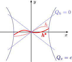
Figure 7: $Q_{h}$-horizontal disc $h^{*}$ obtained from $h$ in terms of Lemma 26.

Lemma 27

Assume that $0<m_{h},m_{v}$ and $m_{h}<1$. Assume that $h$ is a $Q_{v}$-horizontal disc of radius $c\leq 1-\alpha_{v}$ in $N$ and that $Q_{h}(h(\overline{B}_{u}))\geq\alpha_{h}-1.$ Assume also that $f$ satisfies cone conditions for $(Q_{h},m_{h})$ and $(Q_{v},m_{v})$. Let $h^{\ast}$ be the $Q_{v}$-horizontal disc of radius $c^{\ast}=\min\{m_{v}c,c\}$ from Lemma 25. Then $Q_{h}(h^{\ast}(\overline{B}_{u}))\geq\alpha_{h}-1,$ and $h^{\ast}$ is a $Q_{v}$-horizontal disc in $N.$

Proof. Since $\alpha_{h}\in\left(0,1\right),$ $m_{h}\in(0,1)$ and $f$ satisfies cone conditions for $(Q_{h},m_{h}),$ for any $x\in\overline{B}_{u}$

$$Q_{h}(f\circ h(x))\geq m_{h}Q_{h}(h(x))\geq m_{h}\left(\alpha_{h}-1\right)\geq\alpha_{h}-1,$$

which by (17) proves that $Q_{h}(h^{\ast}(\overline{B}_{u}))\geq\alpha_{h}-1$.

The fact that $h^{\ast}$ is in $N$ follows from the facts that $Q_{h}(h^{\ast}(\overline{B}_{u}))\geq\alpha_{h}-1$ and $Q_{v}\left(h^{\ast}(\overline{B}_{u})\right)\leq c^{\ast}=\min\{m_{v}c,c\}\leq c\leq 1-\alpha_{v}$, combined with point 3 from Remark 16.

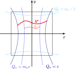
Figure 8: $Q_{h}$-horizontal disc $h^{\ast}$ obtained from $h$ in terms of Lemma 27.

 

5 Construction of the stable and unstable manifolds

In this section we give proofs of Theorems 7, 8.

5.1 Proof of Theorem 7

Proof. We start by considering two points $q^{\ast},q^{\ast\ast}\in W_{\sqrt{m_{v}},N}^{u}$, with backward trajectories $(q_{0}^{\ast},q_{-1}^{\ast},\ldots)$ and $(q_{0}^{\ast\ast},q_{-1}^{\ast\ast},\ldots).$ We will show that:

$$\pi_{x}q^{\ast}=\pi_{x}q^{\ast\ast}\implies q^{\ast}=q^{\ast\ast}.$$ (27)

Since $q^{\ast},q^{\ast\ast}\in W_{\sqrt{m_{v}},N}^{u}$, for any $k\leq 0$

$$\left\|q_{k}^{\ast}\right\|\leq C\left(\sqrt{m_{v}}\right)^{k},\qquad\left\|q_{k}^{\ast\ast}\right\|\leq C\left(\sqrt{m_{v}}\right)^{k}.$$ (28)

On the other hand, since $Q_{h}\left(q^{\ast}-q^{\ast\ast}\right)=-\left\|\pi_{y}\left(q^{\ast}-q^{\ast\ast}\right)\right\|^{2}\leq 0,$ by $\left(Q_{h},m_{h}\right)$ cone conditions we see that for any $k<0\$

$$0 \geq Q_{h}\left(q^{\ast}-q^{\ast\ast}\right)$$

$$=Q_{h}\left(q_{0}^{\ast}-q_{0}^{\ast\ast}\right)$$

$$=Q_{h}\left(f(q_{-1}^{\ast})-f(q_{-1}^{\ast\ast})\right)$$ (29)

$$\geq m_{h}Q_{h}\left(q_{-1}^{\ast}-q_{-1}^{\ast\ast}\right)$$

$$\geq\ldots$$

$$\geq m_{h}^{\left|k\right|}Q_{h}\left(q_{k}^{\ast}-q_{k}^{\ast\ast}\right).$$

This implies that for $k\leq 0$

$$\left\|q_{k}^{\ast}-q_{k}^{\ast\ast}\right\|^{2}\geq\left|Q_{h}\left(q_{k}^{\ast}-q_{k}^{\ast\ast}\right)\right|\geq m_{h}^{k}\left|Q_{h}\left(q^{\ast}-q^{\ast\ast}\right)\right|\geq 0.$$ (30)

Since $m_{v}>m_{h},$ (28) and (30) implies that $q^{\ast}=q^{\ast\ast},$ which proves (27).

We now move to the construction of the function $w^{u}$ from Theorem 7. Let us define a mapping $h_{0}:\overline{B_{u}}\rightarrow N$, as $h_{0}(x)=(x\sqrt{1-\alpha_{v}},0)$. Then $h_{0}$ is a $Q_{h}$-horizontal disc in $N$ and $Q_{v}$-horizontal disk of radius $c=1-\alpha_{v}$. Moreover, for any $x\in\overline{B_{u}}$

$$Q_{h}\left(h_{0}(x)\right)=\alpha_{h}||x\sqrt{1-\alpha_{v}}||^{2}\geq 0>\alpha_{h}-1,$$

which means that assumptions of Lemma 26 are satisfied. Applying inductively Lemma 26, we obtain a sequence of $Q_{h}$-horizontal discs in $N$, that are also $Q_{v}$-horizontal discs of radius $c,$ which we shall denote as $h_{i}$, for $i=0,1,\ldots$. These horizontal disks are given by $h_{i+1}=h_{i}^{\ast}$ in terms of Lemma 25.

We will show that for any $x^{\ast}\in\overline{B}_{u}(0,r^{u})$ there exists a unique point $q^{\ast}$ such that $\pi_{x}q^{\ast}=x^{\ast}$, which lies in $W_{\sqrt{m_{v}},N}^{u}.$ By Lemma 23, for any $i\geq 0$ there exists a point $p_{i}^{\ast}\in h_{i}(\overline{B}_{u})$ such that $\pi_{x}p_{i}^{\ast}=x^{\ast}$. Since $N$ is compact, there exists a convergent subsequence $p_{i_{l}}^{\ast}$ to a point $q^{\ast}(x^{\ast})$

$$\lim_{l\rightarrow\infty}p_{i_{l}}^{\ast}=q^{\ast}\left(x^{\ast}\right),$$ (31)

with $\pi_{x}q^{\ast}(x^{\ast})=x^{\ast}$. We will show that such point is unique, and that it lies in $W_{\sqrt{m_{v}},N}^{u}$. Such point will be the candidate for $w^{u}(x^{\ast})=\pi_{y}q^{\ast}(x^{\ast})$.

We start by showing that there exists a backward trajectory $(q_{0}^{\ast},q_{-1}^{\ast},\ldots)$ in $N\cap\{Q_{h}\geq 0\}$ reaching $q^{\ast}(x^{\ast})$. It is sufficient to show that for any $n\geq 0$ there exists a $q_{-n}^{\ast}$ such that $f^{k}(q_{-n}^{\ast})\in N\cap\{Q_{h}\geq 0\}$ for $k=0,\ldots,n$ and $f^{n}(q_{-n}^{\ast})=q^{\ast}(x^{\ast})$. Let $i\geq n$. Since

$$p_{i}^{\ast}\in h_{i}\left(\overline{B}_{u}\right)=f(h_{i-1}(\overline{B}_{u}))\cap\left\{Q_{v}\leq c\right\},$$

we see that $p_{i}^{\ast}=f(p_{i,-1}^{\ast}),$ with $p_{i,-1}^{\ast}\in h_{i-1}(\overline{B}_{u})$. Since $h_{i-1}$ is a $Q_{h}$-horizontal disc and since $h_{i-1}(0)=0$, we have $p_{i,-1}^{\ast}\in h_{i-1}(\overline{B}_{u})\subset\{Q_{h}\geq 0\}$. Similarly, since

$$p_{i-1}^{\ast}\in h_{i-1}\left(\overline{B}_{u}\right)=f(h_{i-2}(\overline{B}_{u}))\cap\left\{Q_{v}\leq c\right\},$$

we obtain a point $p_{i,-2}^{\ast}\in h_{i-2}(\overline{B}_{u})\subset\{Q_{h}\geq 0\}$ such that $f(p_{i,-2}^{\ast})=p_{i,-1}^{\ast}$. Proceeding inductively we obtain a point $p_{i,-n}^{\ast}$ such that $f^{k}(p_{i,-n}^{\ast})\in N\cap\{Q_{h}\geq 0\}$ and $f^{n}(p_{i,-n}^{\ast})=p_{i}^{\ast}$. Consider now the subsequence $p_{i_{l},-n}^{\ast}$, in terms of $l$, where $i_{l}$ is the subsequence form (31). Since $N\cap\{Q_{h}\geq 0\}$ is compact, there exists a convergent subsequence $p_{i_{l_{m}},-n}^{\ast}$ to a point $q_{-n}^{\ast}$

$$\lim_{m\rightarrow\infty}p_{i_{l_{m}},-n}^{\ast}=q_{-n}^{\ast}.$$

observing that

$$f^{k}(q_{-n}^{\ast}) =\lim_{m\rightarrow\infty}f^{k}(p_{i_{l_{m}},-n}^{\ast})\in N,$$

$$f^{n}(q_{-n}^{\ast}) =\lim_{m\rightarrow\infty}f^{n}(p_{i_{l_{m}},-n}^{\ast})=\lim_{m\rightarrow\infty}p_{i_{l_{m}}}^{\ast}=q^{\ast}(x^{\ast}),$$

we achieve our goal of proving existence of $q_{-n}^{\ast}$. Thus, there exists a backward trajectory in $N\cap\{Q_{h}\geq 0\}$ reaching $q^{\ast}(x^{\ast}).$

Since $q^{\ast}(x^{\ast})$ has a backward trajectory in $N\cap\{Q_{h}\geq 0\}$, by Lemma 17 we see that $q^{\ast}(x^{\ast})\in W_{\sqrt{m_{v}},N}^{u}$.

We now show that the point $q^{\ast}(x^{\ast})$ from (31) is unique. If we take another point $q^{\ast\ast}(x^{\ast})$, then both points $q^{\ast}(x^{\ast})$ and $q^{\ast\ast}(x^{\ast})$ are in $W_{\sqrt{m_{v}},N}^{u}$ and thus by (27) they must coincide. This means that

$$w^{u}(x^{\ast})=\pi_{y}q^{\ast}(x^{\ast})$$

is well defined.

From our construction, for any $x_{1}^{\ast},x_{2}^{\ast}\in\overline{B}_{u}(0,r^{u})$ we have

$$q^{\ast}(x_{1}^{\ast})=\lim_{k\rightarrow\infty}p_{1,k}^{\ast},\qquad\text{and\qquad}q^{\ast}(x_{2}^{\ast})=\lim_{k\rightarrow\infty}p_{2,k}^{\ast},$$

for sequences $p_{1,k}^{\ast},p_{2,k}^{\ast}\in h_{k}(\overline{B}_{u})$. Thus

$$Q_{h}\left(q^{\ast}(x_{1}^{\ast})-q^{\ast}(x_{2}^{\ast})\right)=\lim_{k\rightarrow\infty}Q_{h}\left(p_{1,k}^{\ast}-p_{2,k}^{\ast}\right)\geq 0.$$

This implies that

$$\alpha_{h}||x_{1}^{\ast}-x_{2}^{\ast}||^{2}-||w^{u}(x_{1}^{\ast})-w^{u}(x_{2}^{\ast})||^{2}=Q_{h}(q^{\ast}(x_{1}^{\ast})-q^{\ast}(x_{2}^{\ast}))\geq 0,$$

which proves that $w^{u}$ is Lipschitz with constant $L=\sqrt{\alpha_{h}}$.   

Remark 28

In the proof the constant $C$ from Theorem 7 was established via Lemma 17. In Lemma 17 we see that $C=\sqrt{2\left(1-\alpha_{v}\alpha_{h}\right)^{-1}}$ depends only on the coefficients of the cones $\alpha_{h},\alpha_{v}$.

5.2 Proof of Theorem 8

Proof. Let us fix $y_{0}$ such that $||y_{0}||\leq\sqrt{1-\alpha_{h}}.$ We define a mapping $h_{0}:\overline{B_{u}}\rightarrow N$, as $h_{0}(x)=(x\sqrt{1-\alpha_{v}(1-\left\|y_{0}\right\|^{2})},y_{0})$. Then $h_{0}$ is a $Q_{v}$-horizontal disk in $N$ of radius $c=1-\alpha_{v}>0$. By point 4 from Remark 16, for any $x\in\overline{B_{u}}$

$$Q_{h}\left(x,y_{0}\right)\geq-\left(\sqrt{1-\alpha_{h}}\right)^{2}=\alpha_{h}-1,$$

which means that assumptions of Lemma 27 are satisfied. Applying inductively Lemma 27, we obtain a sequence of $Q_{v}$-horizontal discs, which we shall denote as $h_{i}$, for $i=0,1,\ldots$. These horizontal disks are given by $h_{i+1}=h_{i}^{\ast}$ in terms of Lemma 25. The $h_{i}$ are also $Q_{h}$-horizontal discs for $i>0$.

By construction, we know that $\pi_{x}h_{i}(0)=0$. Let $x_{i}^{\ast}$ be a point such that $f^{i}(h_{0}(x_{i}^{\ast}))=h_{i}(0)$. Since $f$ satisfies cone conditions for $(Q_{v},m_{v})$, for any point $q$ such that $Q_{v}(f(q))\leq 0$, we must have $Q_{v}(q)\leq 0$. This means that since $Q_{v}(h_{i}(0))\leq 0$, we also have $Q_{v}(f^{k}(h_{0}(x_{i}^{\ast})))\leq 0$ for $k=0,\ldots,i$. Since $\overline{B}_{u}$ is compact, there exists a convergent subsequence $x_{i_{m}}^{\ast}$ to some $x^{\ast}\in\overline{B}_{u}$. It means that there exists an $x^{\ast}\in\overline{B}_{u}$ such that

$$f^{i}(h_{0}(x^{\ast}))\in\left\{Q_{v}\leq 0\right\}\cap N\quad\text{for all }i\geq 0.$$ (32)

The point $x^{\ast}$ is a candidate for $w^{s}(y_{0}).$

We now check that $w^{s}(y_{0})$ is well defined. Suppose that

$$f^{i}(h_{0}(x^{\ast\ast}))\in\left\{Q_{v}\leq 0\right\}\cap N\quad\text{for all }i\geq 0.$$ (33)

From Lemma 18 we know that for $C>0,$

$$\left\|f^{i}(h_{0}(x^{\ast}))\right\|\leq C\left(\sqrt{m_{h}}\right)^{i},\qquad\left\|f^{i}(h_{0}(x^{\ast\ast}))\right\|\leq C\left(\sqrt{m_{h}}\right)^{i}.$$ (34)

On the other hand,

$$\left\|f^{i}(h_{0}(x^{\ast}))-f^{i}(h_{0}(x^{\ast\ast}))\right\|^{2} \geq Q_{v}(f^{i}(h_{0}(x^{\ast}))-f^{i}(h_{0}(x^{\ast\ast})))$$

$$\geq m_{v}^{i}Q_{h}(h_{0}(x^{\ast})-h_{0}(x^{\ast\ast}))$$

$$\geq 0.$$

Since $m_{h}<m_{v}$ above inequality and (34) imply that $h_{0}(x^{\ast})=h_{0}(x^{\ast\ast})$.

The same argument can be used to show that any two points $p^{\ast}\neq p^{\ast\ast}$ on the strong stable manifold $W_{\sqrt{m_{h}}}^{s}$ must satisfy

$$Q_{v}\left(p^{\ast}-p^{\ast\ast}\right)\leq 0,$$ (35)

since if this were not the case, we would have

$$\left\|f^{i}(p^{\ast})-f^{i}(p^{\ast\ast})\right\|^{2}\geq Q_{v}(f^{i}(p^{\ast})-f^{i}(p^{\ast\ast}))>m_{v}^{i-1}Q_{h}(f(p^{\ast})-f(x^{\ast\ast}))>0,$$

contradicting contraction at the rate $\sqrt{m_{h}}$.

Observe that by (34), $w^{s}$ parameterizes the stable manifold.

It left to show that $w^{s}$ is Lipschitz with a constant $L=\sqrt{\alpha_{v}}$. By (35)

$$0\geq Q_{v}((w^{s}(y_{1}),y_{1})-(w^{s}(y_{2}),y_{2})),$$

hence

$$||w^{s}(y_{1})-w^{s}(y_{2})||^{2}\leq\alpha_{v}||y_{1}-y_{2}||,$$

as required.   

Remark 29

In the proof, the constant $C$ from Theorem 8 was established via Lemma 18. In Lemma 18 we see that $C=\sqrt{2\left(1-\alpha_{v}\alpha_{h}\right)^{-1}}$ depends only on the coefficients of the cones $\alpha_{h},\alpha_{v}$.

6 Establishing manifolds of ODEs

In this section we consider an ODE

$$p^{\prime}=F(p),$$ (36)

with $F$ of class $C^{1}$, satisfying: for all $p\in N$

$$\left\|F\left(p\right)\right\|\leq\mu,\qquad\left\|DF(p)\right\|\leq L,$$ (37)

and for any $p_{1},p_{2}\in N$

$$\left\|DF\left(p_{1}\right)-DF\left(p_{2}\right)\right\|\leq M\left\|p_{1}-p_{2}\right\|.$$ (38)

Let $\phi_{t}(p)$ stand for the flow induced by (36). We assume that zero is a fixed point.

Definition 30

Let $U$ be a neighborhood of zero and let $\lambda>0$. We say that a set $W_{\lambda,U}^{u}$ consisting of all points $p$ satisfying:

1. $\phi_{t}(p)\in U$ for all $t\leq 0;$

2. there exists a constant $C>0$ (which can depend on $p$), such that for all $t\leq 0$,

   $$\left\|\phi_{t}(p)\right\|\leq Ce^{t\lambda};$$

is a strong unstable manifold with expansion rate $\lambda$ in $U$.

Definition 31

Let $U$ be a neighborhood of zero and let $\lambda<0$. We say that a set $W_{\lambda,U}^{s}$ consisting of all points $p$ satisfying:

1. $\phi_{t}(p)\in U$ for all $t\geq 0;$

2. there exists a constant $C>0$ (which can depend on $p$), such that for all $t\geq 0$,

   $$\left\|\phi_{t}(p)\right\|\leq Ce^{t\lambda};$$ (39)

is a strong stable manifold with contraction rate $\lambda$ in $U.$

Let us assume that

$$\left[DF(N)\right]\subset\left(\begin{array}[c]{cc}\mathbf{A}&\boldsymbol{\varepsilon}_{1}\\ \boldsymbol{\varepsilon}_{2}&\mathbf{B}\end{array}\right),$$

where $\mathbf{A}$, $\mathbf{B}$, $\boldsymbol{\varepsilon}_{1}$ and $\boldsymbol{\varepsilon}_{2}$ are interval matrices. Let $Q_{h}$ and $Q_{v}$ be as defined in (8–9). Assume that we have two constants $c_{h},c_{v}\in\mathbb{R}$ such that for any $A\in\mathbf{A},$ $B\in\mathbf{B}$, $\varepsilon_{1}\in\boldsymbol{\varepsilon}_{1}$ and $\varepsilon_{2}\in\boldsymbol{\varepsilon}_{2}$

$$x^{T}\left(A-\frac{1}{2}\left(\left\|\varepsilon_{1}\right\|+\frac{1}{\alpha_{h}}\left\|\varepsilon_{2}\right\|\right)\mathrm{Id}\right)x >c_{h}\left\|x\right\|^{2},$$ (40)

$$x^{T}\left(A-\frac{1}{2}\left(\left\|\varepsilon_{1}\right\|+\alpha_{v}\left\|\varepsilon_{2}\right\|\right)\mathrm{Id}\right)x >c_{v}\left\|x\right\|^{2},$$ (41)

$$y^{T}\left(B+\frac{1}{2}\left(\left\|\varepsilon_{2}\right\|+\alpha_{h}\left\|\varepsilon_{1}\right\|\right)\mathrm{Id}\right)y <c_{h}\left\|y\right\|^{2},$$ (42)

$$y^{T}\left(B+\frac{1}{2}\left(\left\|\varepsilon_{2}\right\|+\frac{1}{\alpha_{v}}\left\|\varepsilon_{1}\right\|\right)\mathrm{Id}\right)y <c_{v}\left\|y\right\|^{2}.$$ (43)

Theorem 32

Let $r^{u}=\sqrt{1-\alpha_{v}}$ and $U=\overline{B}_{u}(0,r^{u})\times\overline{B}_{s}.$ If $c_{v}>c_{h}$ and $c_{v}>0,$ then there exists a function $w^{u}:\overline{B}_{u}(0,r^{u})\rightarrow\overline{B}_{s},$ such that

$$W_{c_{v},N}^{u}\cap U=\left\{(x,w^{u}(x))|x\in\overline{B}_{u}(0,r^{u})\right\}.$$

Moreover, $w^{u}$ is Lipschitz with a constant $L_{u}=\sqrt{\alpha_{h}}$.

Theorem 33

Let $r^{s}=\sqrt{1-\alpha_{h}}$ and $U=\overline{B}_{u}\times\overline{B}_{s}(0,r^{s}).$ If $c_{h}<c_{v}$ and $c_{h}<0$, then there exists a function $w^{s}:\overline{B}_{s}(0,r^{s})\rightarrow\overline{B}_{u},$ such that

$$W_{c_{h},N}^{s}\cap U=\left\{(w^{s}(y),y)|y\in B_{s}(0,r^{s})\right\}.$$

Moreover, $w^{s}$ is Lipschitz with a constant $L_{s}=\sqrt{\alpha_{v}}.$

Remark 34

Let us note that the assumptions of Theorems 32 and 33 follow directly from the estimates on the vector field. There is no need to integrate the ODE to verify them.

We need some auxiliary results before we give proofs of the theorems at the end of the section. We start with a technical lemma.

Lemma 35

Assume that the vector field satisfies the conditions (37) and (38). Then for

$$g_{1}(p_{1},p_{2},t) =\phi_{t}(p_{1})-\phi_{t}(p_{2})-\left(p_{1}-p_{2}\right),$$

$$g_{2}(p_{1},p_{2},t) =F(\phi_{t}(p_{1}))-F(\phi_{t}(p_{2}))-\left(F(p_{1})-F(p_{2})\right),$$

we have the following estimates

$$\left\|g_{1}\left(p_{1},p_{2},t\right)\right\| \leq\left(e^{\left|t\right|L}-1\right)\left\|p_{1}-p_{2}\right\|,$$ (44)

$$\left\|g_{2}\left(p_{1},p_{2},t\right)\right\| \leq\left(L\left(e^{L\left|t\right|}-1\right)+\left|t\right|e^{L\left|t\right|}\mu M\right)\left\|p_{1}-p_{2}\right\|.$$ (45)

Proof. The proof is given in Appendix 10.5.   

The following lemma will be the key for the proof of Theorems 32 and 33.

Lemma 36

Let $Q(x,y)=\alpha\left\|x\right\|^{2}-\beta\left\|y\right\|^{2}$ with $\alpha,\beta>0$. Assume that for $c\in\mathbb{R}$ and any $A\in\mathbf{A},$ $B\in\mathbf{B}$, $\varepsilon_{1}\in\boldsymbol{\varepsilon}_{1}$ and $\varepsilon_{2}\in\boldsymbol{\varepsilon}_{2}$ holds

$$x^{T}\left(A-\frac{1}{2}\left(\left\|\varepsilon_{1}\right\|+\frac{\beta}{\alpha}\left\|\varepsilon_{2}\right\|\right)\mathrm{Id}\right)x >c\left\|x\right\|^{2},$$ (46)

$$y^{T}\left(B+\frac{1}{2}\left(\left\|\varepsilon_{2}\right\|+\frac{\alpha}{\beta}\left\|\varepsilon_{1}\right\|\right)\mathrm{Id}\right)y <c\left\|y\right\|^{2}.$$ (47)

Then for sufficiently small $t>0,$ the map $\phi_{t}$ satisfies cone conditions in $N$ for $(Q,m=1+t2c).$

Remark 37

Conditions (46), (47) hold when the two matrixes

$$A-\frac{1}{2}\left(\left\|\varepsilon_{1}\right\|+\frac{\beta}{\alpha}\left\|\varepsilon_{2}\right\|+2c\right)\mathrm{Id},$$

$$- B+\frac{1}{2}\left(-\left\|\varepsilon_{2}\right\|-\frac{\alpha}{\beta}\left\|\varepsilon_{1}\right\|+2c\right)\mathrm{Id}\mathbf{,}$$

are strictly positive definite. The same approach can be used to verify (40)–(43).

Proof. (of Lemma 36) Let $g_{1}$ and $g_{2}$ be the functions defined in Lemma 35. Let $\mathcal{Q}$ denote the $\left(u+s\right)\times\left(u+s\right)$ matrix associated with $Q$, that is, $Q(p)=p^{T}\mathcal{Q}p$, and let

$$C=\int_{0}^{1}DF\left(\left(1-t\right)p_{2}+tp_{1}\right)dt\in\left[DF(N)\right].$$

We can compute

$$\frac{d}{dt}Q\left(\phi_{t}(p_{1})-\phi_{t}(p_{2})\right)$$ (48)

$$=\left(\phi_{t}^{\prime}(p_{1})-\phi_{t}^{\prime}(p_{2})\right)^{T}\mathcal{Q}\left(\phi_{t}(p_{1})-\phi_{t}(p_{2})\right)$$

$$\quad+\left(\phi_{t}(p_{1})-\phi_{t}(p_{2})\right)^{T}\mathcal{Q}\left(\phi_{t}^{\prime}(p_{1})-\phi_{t}^{\prime}(p_{2})\right)$$

$$=\left(F(\phi_{t}(p_{1}))-F(\phi_{t}(p_{2}))\right)^{T}\mathcal{Q}\left(\phi_{t}(p_{1})-\phi_{t}(p_{2})\right)$$

$$\quad+\left(\phi_{t}(p_{1})-\phi_{t}(p_{2})\right)^{T}\mathcal{Q}\left(F(\phi_{t}(p_{1}))-F(\phi_{t}(p_{2}))\right)$$

$$=\left(F(p_{1})-F(p_{2})+g_{2}\left(p_{1},p_{2},t\right)\right)^{T}\mathcal{Q}\left(p_{1}-p_{2}+g_{1}\left(p_{1},p_{2},t\right)\right)$$

$$\quad+\left(p_{1}-p_{2}+g_{1}\left(p_{1},p_{2},t\right)\right)^{T}\mathcal{Q}\left(F(p_{1})-F(p_{2})+g_{2}\left(p_{1},p_{2},t\right)\right)$$

$$=\left(p_{1}-p_{2}\right)^{T}\left(C^{T}\mathcal{Q}+\mathcal{Q}C\right)\left(p_{1}-p_{2}\right)+g_{3}(p_{1},p_{2},t),$$

where by (44–45) we see that for any $p_{1},p_{2}\in N$ and $\left|t\right|\leq 1$

$$\left\|g_{3}(p_{1},p_{2},t)\right\|\leq bt\left\|p_{1}-p_{2}\right\|^{2},$$

for a constant $b$ dependent on $\mu,L,M,\alpha$ and $\beta$.

Since $C\in\left[DF(N)\right]$, it is of the form

$$C=\left(\begin{array}[c]{cc}A&\varepsilon_{1}\\ \varepsilon_{2}&B\end{array}\right),$$

with $A\in\mathbf{A},$ $B\in\mathbf{B},$ $\varepsilon_{1}\in\boldsymbol{\varepsilon}_{1}$ and $\varepsilon_{2}\in\boldsymbol{\varepsilon}_{2}$. Using the fact that

$$x^{T}\varepsilon_{i}y\geq-\left\|\varepsilon_{i}\right\|\left\|x\right\|\left\|y\right\|\geq-\frac{1}{2}\left\|\varepsilon_{i}\right\|\left(x^{T}x+y^{T}y\right)\quad\text{for }i=1,2$$

for $p=\left(x,y\right)\neq 0$ we can compute

$$p^{T}\mathcal{Q}Cp =\alpha x^{T}Ax+\alpha x^{T}\varepsilon_{1}y-\beta y^{T}\varepsilon_{2}x-\beta y^{T}By$$ (49)

$$\geq\alpha x^{T}Ax-\alpha\frac{1}{2}\left\|\varepsilon_{1}\right\|\left(x^{T}x+y^{T}y\right)$$

$$-\beta\frac{1}{2}\left\|\varepsilon_{2}\right\|\left(x^{T}x+y^{T}y\right)-\beta y^{T}By$$

$$=\alpha x^{T}\left(A-\frac{1}{2}\left(\left\|\varepsilon_{1}\right\|+\frac{\beta}{\alpha}\left\|\varepsilon_{2}\right\|\right)\mathrm{Id}\right)x$$

$$-\beta y^{T}\left(B+\frac{1}{2}\left(\left\|\varepsilon_{2}\right\|+\frac{\alpha}{\beta}\left\|\varepsilon_{1}\right\|\right)\mathrm{Id}\right)y$$

$$>\alpha c\left\|x\right\|^{2}-\beta c\left\|y\right\|^{2}$$

$$=cp^{T}\mathcal{Q}p.$$

Similarly, it follows that for $p\neq 0$

$$p^{T}C^{T}\mathcal{Q}p>cp^{T}\mathcal{Q}p.$$ (50)

Combining (48), (49) and (50), taking $p_{1}\neq p_{2}$, for some $\xi\in\left[-t,t\right]$ (which depends on $p_{1},p_{2}$ and $t$),

$$Q\left(\phi_{t}(p_{1})-\phi_{t}(p_{2})\right)$$

$$=Q\left(\phi_{t}(p_{1})-\phi_{t}(p_{2})\right)|_{t=0}+t\left.\frac{d}{ds}Q\left(\phi_{s}(p_{1})-\phi_{s}(p_{2})\right)\right|_{s=\xi}$$

$$=Q\left(p_{1}-p_{2}\right)+t\left(p_{1}-p_{2}\right)^{T}\left(C^{T}\mathcal{Q}+\mathcal{Q}C\right)\left(p_{1}-p_{2}\right)+tg_{3}(p_{1},p_{2},\xi)$$

$$>\left(1+2tc\right)Q\left(p_{1}-p_{2}\right)+tg_{3}(p_{1},p_{2},\xi).$$

Since

$$\left\|tg_{3}(p_{1},p_{2},\xi)\right\|\leq bt^{2}\left\|p_{1}-p_{2}\right\|^{2},$$

we see that for sufficiently small $\left|t\right|$

$$Q\left(\phi_{t}(p_{1})-\phi_{t}(p_{2})\right)\geq\left(1+2tc\right)Q\left(p_{1}-p_{2}\right),$$

as required.   

We are now ready to prove Theorems 32 and 33.

Proof of Theorem 32. From Lemma 36 it follows that there exists a $\tau^{\ast}$ such that for any $\tau\in\left(0,\tau^{\ast}\right)$ the time shift along the trajectory map $\phi_{\tau}$ satisfies cone conditions for $\left(Q_{h},m_{h}\right)$ and $\left(Q_{v},m_{v}\right),$ with

$$m_{h} =m_{h}(\tau)=1+\tau 2c_{h},$$

$$m_{v} =m_{v}(\tau)=1+\tau 2c_{v}.$$

We can choose $\tau^{\ast}$ small enough so that $m_{h}(\tau)>0,$ for $\tau\in\left(0,\tau^{\ast}\right)$. Also, since $c_{v}>0$, we see that $m_{v}(\tau)>1$. By Theorem 7, there exists a strong unstable manifold for $\phi_{\tau}$, such that $W_{\sqrt{m_{v}(\tau)},N}^{u}\cap U$ is a graph of a function $w^{u,\tau}:\overline{B}_{u}(0,r)\rightarrow\overline{B}_{s}.$

We will now show that for $\tau_{1},\tau_{2}\in\left(0,\tau^{\ast}\right)$ we have $w^{u,\tau_{1}}=w^{u,\tau_{2}}$. Assume that $\tau_{1}<\tau_{2}$. Let us fix $x\in\overline{B}_{u}(0,r)$ and define $p_{1}=w^{u,\tau_{1}}(x),$ $p_{2}=w^{u,\tau_{2}}(x)$. We will show that $p_{1}=p_{2}$. In our argument we will use the fact that

$$1\leq\left(1+\frac{b}{a}\right)^{\frac{a}{2}}\leq\left(1+b\right)^{\frac{1}{2}}\qquad\text{for }a\in(0,1],\text{ and }b>0.$$ (51)

Let $n\in\mathbb{N}$ be fixed. Since $\tau_{1}<\tau_{2}$, there exists a $k\in\mathbb{N}$, $k>n$ and $\delta\in\left[0,\tau_{1}\right)$, such that

$$n\tau_{2}=k\tau_{1}-\delta.$$

From (51), by taking $b=2c_{v}\tau_{1}$ and $a=\frac{n}{k},$ follows that

$$\left(1+2c_{v}\frac{k}{n}\tau_{1}\right)^{-\frac{n}{2}}\geq\left(1+2c_{v}\tau_{1}\right)^{-\frac{k}{2}},$$

which gives

$$\left(\sqrt{m_{v}(\tau_{2})}\right)^{-n}=\left(1+2c_{v}\tau_{2}\right)^{-\frac{n}{2}}\geq\left(1+2c_{v}\frac{k}{n}\tau_{1}\right)^{-\frac{n}{2}}\\ \geq\left(1+2c_{v}\tau_{1}\right)^{-\frac{k}{2}}=\left(\sqrt{m_{v}(\tau_{1})}\right)^{-k}.$$

From this estimate we see that

$$\left\|\left(\phi_{\tau_{2}}\right)^{-n}\left(p_{1}\right)\right\|=\left\|\phi_{-n\tau_{2}}\left(p_{1}\right)\right\|=\left\|\phi_{\delta}\circ\phi_{-k\tau_{1}}\left(p_{1}\right)\right\|\\ \leq e^{L\delta}\left\|\phi_{-k\tau_{1}}\left(p_{1}\right)\right\|\leq e^{L\tau_{1}}C\sqrt{m_{v}(\tau_{1})}^{-k}\leq e^{L\tau_{1}}C\sqrt{m_{v}(\tau_{2})}^{-n},$$

which means that $p_{1}$ is on the strong unstable manifold for the map $\phi_{\tau_{2}}$, hence $p_{1}=p_{2},$ as required.

Since the strong unstable manifold for the time shift maps $\phi_{\tau}$ is independent of the choice of $\tau$, we see that it coincides with a strong unstable manifold for the flow $\phi_{t}$. What remains is to prove that the expansion rate for this manifold is $c_{v}$.

For $\tau\in\left(0,\tau^{\ast}\right)$ the map $\phi_{\tau}$ satisfies cone conditions for $\left(Q_{h},m_{h}(\tau)\right)$ and $\left(Q_{v},m_{v}(\tau)\right)$ (where $Q_{h}$ and $Q_{v}$ are the same for all $\tau$), hence by Remark 28,

$$\left\|\left(\phi_{\tau}\right)^{-n}(p)\right\|\leq C\sqrt{m_{v}(\tau)}^{-n},$$

for $C$ which is independent of $\tau$. Let $t<0$. The expansion rate condition follows by computing

$$\left\|\phi_{t}(p)\right\| =\left\|\left(\phi_{\frac{\left|t\right|}{n}}\right)^{-n}(p)\right\|$$

$$\leq C\left(\sqrt{m_{v}\left(\left|t\right|/n\right)}\right)^{-n}$$ (52)

$$=C\left(1+\frac{2}{n}\left|t\right|c_{v}\right)^{-\frac{n}{2}}\overset{n\rightarrow+\infty}{\rightarrow}Ce^{tc_{v}},$$

as required.   

Proof of Theorem 33. The result follows from combining Lemma 36 with Theorem 8, and mirror arguments to the proof of Theorem 32.   

7 Proof of a homoclinic connection in the restricted three body problem

7.1 A suitable change of coordinates

To verify assumptions of Theorem 32 close to $L_{1}$ we consider the PCR3BP in suitable local coordinates. These are introduced below in two steps. The first step takes the linearized vector field into a Jordan form, through a linear change of coordinates. The second step involves a nonlinear change of coordinates, which further “straightens out” the unstable coordinate.

We now discuss the linear change of coordinates. The libration point is of the form

$$L_{1}^{\mu}=\left(x_{L_{1}}^{\mu},0,0,x_{L_{1}}^{\mu}\right).$$

The Jacobian of the vector field has an unstable eigenvalue, which we denote as $\lambda.$ We consider the following linear change of coordinates ([20], Section 2.1)

$$C^{\mu}=\left(\begin{array}[c]{cccc}\frac{2\lambda}{s_{1}}&\frac{-2\lambda}{s_{1}}&0&\frac{2v}{s_{2}}\\ \frac{\lambda^{2}-2c_{2}-1}{s_{1}}&\frac{\lambda^{2}-2c_{2}-1}{s_{1}}&\frac{-v^{2}-2c_{2}-1}{s_{2}}&0\\ \frac{\lambda^{2}+2c_{2}+1}{s_{1}}&\frac{\lambda^{2}+2c_{2}+1}{s_{1}}&\frac{-v^{2}+2c_{2}+1}{s_{2}}&0\\ \frac{\lambda^{3}+(1-2c_{2})\lambda}{s_{1}}&\frac{-\lambda^{3}-(1-2c_{2})\lambda}{s_{1}}&0&\frac{-v^{3}+(1-2c_{2})v}{s_{2}}\end{array}\right)$$ (53)

where

$$c_{2} =\frac{1}{\gamma^{3}}\left(\mu+\frac{(1-\mu)\gamma^{3}}{(1-\gamma)^{3}}\right),$$

$$\gamma =x_{L_{1}}^{\mu}+1-\mu,$$

$$s_{1} =\sqrt{2\lambda\left(\left(4+3c_{2}\right)\lambda^{2}+4+5c_{2}-6c_{2}^{2}\right)},$$

$$s_{2} =\sqrt{v\left(\left(4+3c_{2}\right)v^{2}-4-5c_{2}+6c_{2}^{2}\right)},$$

that puts the linear terms of the vector field at $L_{1}^{\mu}$ into the Jordan form

$$\left(\begin{array}[c]{cccc}\lambda&0&0&0\\ 0&-\lambda&0&0\\ 0&0&0&v\\ 0&0&-v&0\end{array}\right).$$

We note that in the above, for sake of keeping the notations short, we have omitted the dependence of parameters on $\mu.$ In fact, for different $\mu,$ each nonzero entry of $C^{\mu}$ is different.

Using the notation $\mathbf{x}=\left(X,Y,P_{X},P_{Y}\right)$ for the original coordinates of the problem, we introduce local coordinates $\mathbf{v}$ at $L_{1}^{\mu}$ as

$$\mathbf{x}=L_{1}^{\mu}+C^{\mu}\mathbf{v.}$$

In coordinates $\mathbf{v}$, the vector field is

$$\tilde{F}(\mathbf{v})=\left(C^{\mu}\right)^{-1}F\left(L_{1}^{\mu}+C^{\mu}\mathbf{v}\right),$$

and the Jacobian of the vector field at zero is

$$D\tilde{F}(0)=\text{diag}\left(A_{h},A_{c}\right),$$

with

$$A_{h}=\begin{pmatrix}\lambda&0\\ 0&-\lambda\end{pmatrix}\qquad\text{and }\qquad A_{c}=\left(\begin{array}[c]{cc}0&v\\ -v&0\end{array}\right).$$

The matrix $A_{h}$ represents the linearized hyperbolic dynamics, and $A_{c}$ represents the center rotation at the fixed point.

The second step is to consider a nonlinear change of coordinates. To do so let us consider an equation

$$\tilde{F}(K(\mathsf{x}))=R(\mathsf{x})\,DK(\mathsf{x}),$$ (54)

where $K:\mathbb{R}\rightarrow\mathbb{R}^{4}$ and $R:\mathbb{R}\rightarrow\mathbb{R}$ are analytic. We refer to (54) as the cohomology equation. The graph of $K$ parametrizes the unstable manifold at the fixed point. An approximate solution of $K$ and $R$ can be found numerically (for details see [5]). We use a polynomial $K$, which is an approximate, numerically obtained solution of (54), and use it to define the following nonlinear change of coordinates

$$\psi=\left(\psi_{0},\psi_{1},\psi_{2},\psi_{3}\right):\mathbb{R}^{4}\rightarrow\mathbb{R}^{4},$$

where

$$\psi_{0}\left(\mathsf{x},\mathsf{y}_{1},\mathsf{y}_{2},\mathsf{y}_{3}\right) =K_{0}(\mathsf{x})-\left(\mathsf{y}_{1}K_{1}^{\prime}(\mathsf{x})+\mathsf{y}_{2}K_{2}^{\prime}(\mathsf{x})+\mathsf{y}_{3}K_{3}^{\prime}(\mathsf{x})\right),$$ (55)

$$\psi_{i}\left(\mathsf{x},\mathsf{y}_{1},\mathsf{y}_{2},\mathsf{y}_{3}\right) =K_{i}(\mathsf{x})+\mathsf{y}_{i}K_{0}^{\prime}(\mathsf{x})\quad\text{for }i=1,2,3.$$

Note that since the graph of $K$ approximates the unstable manifold, $\psi(\mathsf{x},0)=K(\mathsf{x})$ gives points close to the unstable manifold of the fixed point. The intuitive idea behind (55) is to arrange the coordinates so that $\psi\left(\mathsf{x},\mathsf{y}_{1},\mathsf{y}_{2},\mathsf{y}_{3}\right)-K(\mathsf{x})$ is orthogonal to $K^{\prime}(\mathsf{x})$ (see Figure 9).

Figure 9: The unstable manifold in coordinates $\mathbf{q=}(\mathsf{x},\mathsf{y}_{1},\mathsf{y}_{2},\mathsf{y}_{3})$ (left), and in coordinates $\mathbf{v}$ (right).

Combining the linear and nonlinear changes of coordinates gives the total change $\Phi:$ $\mathbb{R}^{4}\rightarrow\mathbb{R}^{4}$ from coordinates $\mathbf{q}=\left(\mathsf{x},\mathsf{y}_{1},\mathsf{y}_{2},\mathsf{y}_{3}\right),$ defined as

$$\mathbf{x}=\Phi^{\mu}(\mathbf{q}):=C^{\mu}\psi\left(\mathbf{q}\right).$$ (56)

The vector field in coordinates $\mathbf{q}$ is

$$\hat{F}(\mathbf{q})=D\left(\Phi^{\mu}\right)^{-1}\left(\Phi^{\mu}(\mathbf{q})\right)F\left(\Phi^{\mu}(\mathbf{q})\right).$$ (57)

Remark 38

In our application, the nonlinear change of coordinates is not strictly necessary. Even without it we can obtain our result, but with smaller accuracy. We decided to add the nonlinear change in order to demonstrate that such techniques are possible. Also, with a nonlinear change of coordinates some more careful consideration is needed when computing the derivative of the vector field in local coordinates. This is discussed in section 7.2.

7.2 Enclosure of the unstable manifold

In order to obtain an enclosure of the unstable manifold in coordinates $\mathbf{q}$ we apply Theorem 32 to establish the existence of the manifold.

Let us first specify our change of coordinates $\Phi^{\mu}$ (see (56)). The linear part $C^{\mu}$ of $\Phi^{\mu}$ is given by (53). We consider an interval of parameters

$$\boldsymbol{\mu}=0.004253863522+10^{-10}\left[-1,1\right],$$

and for any $\mu\in\boldsymbol{\mu}$ take the same nonlinear change $\psi$ (see (55)), with $K$ chosen as

$$K_{0}\left(\mathsf{x}\right) =\mathsf{x},$$ (58)

$$K_{1}\left(\mathsf{x}\right) =-0.4426997319120566\mathsf{x}^{2}+0.2117307906593041\mathsf{x}^{3},$$

$$K_{2}\left(\mathsf{x}\right) =0.7204702544171099\mathsf{x}^{2}-0.2077414984788253\mathsf{x}^{3},$$

$$K_{3}\left(\mathsf{x}\right) =0.6096754412253178\mathsf{x}^{2}-1.6248371332133488\mathsf{x}^{3}.$$

The first step is to obtain an enclosure of the fixed point in local coordinates $\mathbf{q}$ (see (56)). We do this by applying the interval Newton method (Theorem 1). In order to do this we have to compute the derivative of the local vector field (57) as follows. Since

$$D\left(\left(\Phi^{\mu}\right)^{-1}\right)\left(\Phi^{\mu}\left(\mathbf{q}\right)\right)=\left(D\Phi^{\mu}\left(\mathbf{q}\right)\right)^{-1},$$

we see that

$$D\Phi^{\mu}\left(\mathbf{q}\right)\hat{F}(\mathbf{q})=F\left(\Phi^{\mu}(\mathbf{q})\right).$$

Differentiating on both sides gives

$$D^{2}\Phi^{\mu}\left(\mathbf{q}\right)\hat{F}(\mathbf{q})+D\Phi^{\mu}\left(\mathbf{q}\right)D\hat{F}(\mathbf{q})=DF\left(\Phi^{\mu}(\mathbf{q})\right)D\Phi^{\mu}(\mathbf{q}),$$

hence

$$D\hat{F}(\mathbf{q})=\left(D\Phi^{\mu}\left(\mathbf{q}\right)\right)^{-1}\left(DF\left(\Phi^{\mu}(\mathbf{q})\right)D\Phi^{\mu}(\mathbf{q})-D^{2}\Phi^{\mu}\left(\mathbf{q}\right)\hat{F}(\mathbf{q})\right).$$ (59)

The main advantage of this approach is that we do not need to invert $\Phi^{\mu}$ to apply (59). Using (59) and Theorem 1 we can establish that for all $\mu\in\boldsymbol{\mu}$ the fixed point is in a set which we denote as $B$.

The second step is to verify assumptions of Theorem 7 using Lemma 36. In order to do so we choose $\alpha_{h},\alpha_{v}$, and take

$$N=B+\left[0,r_{u}\right]\times\left[-r_{u}\sqrt{\alpha_{h}},r_{u}\sqrt{\alpha_{h}}\right]^{3}.$$ (60)

To obtain a good enclosure we subdivide the set $N$, and compute the derivative on smaller subsets. Numerical results are listed in section 7.4. The unstable manifold expressed in local coordinates $\mathbf{q}$ passes through (see Figure 10)

$$U=B+\{\sqrt{1-\alpha_{v}}\}\times\left[-\sqrt{\alpha_{h}},\sqrt{\alpha_{h}}\right]^{3}.$$ (61)

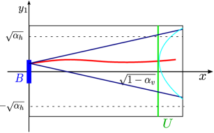
Figure 10: The unstable manifold expressed in local coordinates (in red) passes through a box $U$ (in green). The enclosure $B$ of a fixed point is a small blue box around $0$.

7.3 Proof of existence of a homoclinic connection

Let $U_{\mu}$ be a set which contains a point on the unstable manifold of $L_{1}^{\mu}.$ Assume that for any $\mu\in\boldsymbol{\mu}$ the Poincaré map

$$P_{\mu} :U_{\mu}\rightarrow\{y=0\},$$

$$P_{\mu}(\mathbf{x}) :=\phi_{\tau(\mathbf{x})}(\mathbf{x}),$$ (62)

where

$$\tau\left(\mathbf{x}\right)=\inf\left\{t|t>0,\phi_{t}(\mathbf{x})\in\{y=0\}\right\},$$

is well defined.

Lemma 39

Assume that $\boldsymbol{\mu}=\left[\mu_{\mathrm{left}},\mu_{\mathrm{right}}\right].$If

$$\pi_{p_{x}}P_{\mu_{\mathrm{left}}}(\mathbf{x}) <0,\quad\text{for any }\mathbf{x}\in U_{\mu_{\mathrm{left}}},$$ (63)

$$\pi_{p_{x}}P_{\mu_{\mathrm{right}}}(\mathbf{x}) >0,\quad\text{for any }\mathbf{x}\in U_{\mu_{\mathrm{right}}},$$ (64)

then there exists a $\mu\in\left(\mu_{\mathrm{left}},\mu_{\mathrm{right}}\right)$, for which we have a homoclinic orbit to $L_{1}^{\mu}.$

Proof. Let $\mathbf{x}_{\mu}$ be any point from the intersection of $U_{\mu}$ with $W^{u}(L_{1}^{\mu}).$ If

$$P_{\mu}(\mathbf{x}_{\mu})=\left(x,0,0,p_{y}\right),$$ (65)

for some $x,p_{y}$ (which depend on $\mu$), then the point $P_{\mu}(\mathbf{x}_{\mu})$ is $S$-symmetric (see (4)), and by (5)

$$S(\phi_{t}(P_{\mu}(\mathbf{x}_{\mu})))=\phi_{-t}(S(P_{\mu}(\mathbf{x}_{\mu})))=\phi_{-t}(P_{\mu}(\mathbf{x}_{\mu}))\overset{t\rightarrow+\infty}{\rightarrow}L_{1}^{\mu}.$$

This means that $P_{\mu}(\mathbf{x}_{\mu})$ lies on a homoclinic orbit to $L_{1}^{\mu}.$

We need to prove that there exists a parameter $\mu\in\boldsymbol{\mu},$ for which $P_{\mu}(\mathbf{x}_{\mu})$ would be of the form (65). By definition of $P_{\mu}$ (62), we know that $\pi_{y}P_{\mu}(\mathbf{x}_{\mu})=0.$ It is therefore sufficient to show that for some $\mu\in\left(\mu_{\mathrm{left}},\mu_{\mathrm{right}}\right)$

$$\pi_{p_{x}}P_{\mu}(\mathbf{x}_{\mu})=0.$$

Let

$$g:\left[\mu_{\mathrm{left}},\mu_{\mathrm{right}}\right]\rightarrow\mathbb{R}$$

be defined as

$$g(\mu)=\pi_{p_{x}}P_{\mu}(\mathbf{x}_{\mu}).$$

By (63–64) we see that $g(\mu_{\mathrm{left}})<0<g(\mu_{\mathrm{right}})$. By continuity of the flow with respect to the parameters of the vector field, we know that $g$ is continuous, hence existence of $\mu$ for which $g(\mu)=0$ follows from the Bolzano theorem.   

For a given $\mu\in\boldsymbol{\mu}$ we can obtain the enclosure $U_{\mu}$ using the method described in section 7.2. In fact, the method can be applied not only for a single parameter $\mu\in\boldsymbol{\mu}$, but for an interval of parameters. Conditions (63–64) can be verified by integrating the system numerically, using a rigorous, interval arithmetic based integrator. Such tool is available as a part of the CAPD library. The package can compute Poincaré maps $P_{\mu}$ on prescribed parameter intervals. As the Poincaré map is computed, at the same time it is verified that it is well defined.

7.4 Computer assisted bounds

Let us first take

$$\mu_{\mathrm{left}}=0.004253863522-10^{-10}.$$

In local coordinates $\mathbf{q}$, the enclosure $B$ for the fixed point is

$$B=10^{-15}\left(\begin{array}[c]{c}[-1.137,1.169]\\ [-0.426,0.394]\\ [-0.181,0.181]\\ [-0.180,0.308]\end{array}\right).$$

For the enclosure $N$ of the unstable manifold (60) in coordinates $\mathbf{q}$ we take

$$\alpha_{h}=10^{-8},\qquad\alpha_{v}=10^{-4},\qquad r_{u}=10^{-7}.$$

The enclosure (displayed with rough rounding, which ensures true enclosure) of the derivative of the vector field in local coordinates is

$$\left[D\hat{F}(N)\right]=$$

$$\left(\begin{array}[c]{cccc}\text{{\footnotesize[2.80038,2.80039]}}&\text{{\footnotesize 10}}^{\text{{\footnotesize-6}}}\text{{\footnotesize[-0.0065,1.281]}}&\text{{\footnotesize 10}}^{\text{{\footnotesize-9}}}\text{{\footnotesize[-1.469,1.468]}}&\text{{\footnotesize 10}}^{\text{{\footnotesize-7}}}\text{{\footnotesize[-6.752,0.032]}}\\ \text{{\footnotesize 10}}^{\text{{\footnotesize-9}}}\text{{\footnotesize 8.521[-1,1]}}&\text{{\footnotesize[-2.80039,-2.80038]}}&\text{{\footnotesize 10}}^{\text{{\footnotesize-6}}}\text{{\footnotesize[-0.0015,1.01]}}&\text{{\footnotesize 10}}^{\text{{\footnotesize-7}}}\text{{\footnotesize[-5.352,0.032]}}\\ \text{{\footnotesize 10}}^{\text{{\footnotesize-9}}}\text{{\footnotesize 6.035[-1,1]}}&\text{{\footnotesize 10}}^{\text{{\footnotesize-7}}}\text{{\footnotesize[-6.752,0.0320]}}&\text{{\footnotesize 10}}^{\text{{\footnotesize-7}}}\text{{\footnotesize[-2.659,0.0044]}}&\text{{\footnotesize[2.25179,2.25180]}}\\ \text{{\footnotesize 10}}^{\text{{\footnotesize-9}}}\text{{\footnotesize 4.053[-1,1]}}&\text{{\footnotesize 10}}^{\text{{\footnotesize-9}}}\text{{\footnotesize[-1.468,1.469]}}&\text{{\footnotesize[-2.25180,-2.25179]}}&\text{{\footnotesize 10}}^{\text{{\footnotesize-7}}}\text{{\footnotesize[-0.0044,2.66]}}\end{array}\right)$$

To apply Theorem 32 we take $c_{v}=2.8$ (which looking at $[D\hat{F}(N)]$ is clearly close to its unstable eigenvalue) and $c_{h}=1$ (here we arbitrarily chose a number from $(0,c_{v})$), and verify conditions (40–43).

The set $U$ defined in (61), when transported to the original coordinates is equal to (displayed with rough rounding, which ensures true enclosure)

$$U_{\mu_{\mathrm{left}}}=L_{1}^{\mu_{\mathrm{left}}}+10^{-8}\left(\begin{array}[c]{c}[4.007,4.008]\\ [-1.934,-1.931]\\ [13.15,13.16]\\ [-1.407,-1.402]\end{array}\right).$$

This shows that we enclose the unstable manifold very close to the fixed point.

After propagating the set $U_{\mu_{{}_{\mathrm{left}}}}$ to the section $\{y=0\}$ we obtain an estimate on the image by the Poincaré map

$$\left[P_{\mu_{{}_{\mathrm{left}}}}\left(U_{\mu_{{}_{\mathrm{left}}}}\right)\right]=\left(\begin{array}[c]{c}0.8270258829+10^{-10}\left[-1,1\right]\\ 0\\ -10^{-8}[7.501,2.915]\\ 0.9251225636+10^{-10}\left[-1,1\right]\end{array}\right).$$

The important result is that on the third coordinate we have values smaller than zero, which verifies (63).

For

$$\mu_{\mathrm{right}}=0.004253863522+10^{-10},$$

up to the rounding used to present the result in this paper, the estimates on $B$ and $[D\hat{F}(N)]$ are indistinguishable from the ones for $\mu_{\mathrm{left}}$. The important fact though is that

$$\left[P_{\mu_{{}_{\mathrm{right}}}}\left(U_{\mu_{{}_{\mathrm{right}}}}\right)\right]=\left(\begin{array}[c]{c}0.82702588075+10^{-10}\left[-1,1\right]\\ 0\\ 10^{-8}[2.825,7.421],\\ 0.9251225623+10^{-10}\left[-1,1\right]\end{array}\right),$$

is positive on the third coordinate, which ensures (64).

To verify that $P_{\mu}$ is well defined for all $\mu\in\boldsymbol{\mu}$, similar computations, but with lesser accuracy, were performed.

The computer assisted proof takes 4.27 seconds, on a single core Intel i7 processor, with 1.90GHz. Majority of this time was spent on verifying that $P_{\mu}$ is well defined for all $\mu\in\boldsymbol{\mu}$. In order to do so, the parameter interval was subdivided into 20 fragments $\boldsymbol{\mu}=\boldsymbol{\mu}_{1}\cup\ldots,\cup\boldsymbol{\mu}_{20}$, and each time we needed to integrate from $U_{\boldsymbol{\mu}_{i}}$ to the section $\{y=0\},$ for $i=1,\ldots,20,$ which was time consuming.

8 Closing remarks

The paper presents a new method for establishing of strong (un)stable manifolds for fixed points. The method can be applied for computer assisted proofs. We have shown an application of our method in the context of the planar circular restricted three body problem, proving that there exists a homoclinic orbit to the libration point $L_{1}$ for a suitably chosen mass parameter. Our method produced a tight enclosure of the manifold and also a tight enclosure for the mass parameter for which the manifold leads to a homoclinic connection.

9 Acknowledgements

We would like to thank Piotr Zgliczyński for reading our work and for very helpful comments and corrections. We also thank Rafael de la Llave for discussions concerning the application of the parameterization method. We thank him also for his C code, that we have used to obtain the suitable change of coordinates in the application of our method for the restricted three body problem. All the computer assisted proofs presented in this paper have been performed using the CAPD library. We thank Tomasz Kapela and Daniel Wilczak for discussions concerning the use of the library. Finally, we thank the anonymous referee for very helpful comments, which have enabled us to improve the paper.

10 Appendix

10.1 Proof of Lemma 10

Proof. For any $q^{\ast},q^{\ast\ast}\in N$

$$\frac{d}{dt}f(\left(1-t\right)q^{\ast\ast}+tq^{\ast})=Df\left(\left(1-t\right)q^{\ast\ast}+tq^{\ast}\right)\left(q^{\ast}-q^{\ast\ast}\right),$$

hence

$$f(q^{\ast})-f\left(q^{\ast\ast}\right)=\int_{0}^{1}Df\left(\left(1-t\right)q^{\ast\ast}+tq^{\ast}\right)dt\left(q^{\ast}-q^{\ast\ast}\right).$$

Since

$$B=\int_{0}^{1}Df\left(\left(1-t\right)q^{\ast\ast}+tq^{\ast}\right)dt\in\left[Df\left(N\right)\right],$$

we see that for $q^{\ast}\neq q^{\ast\ast}$

$$Q\left(f(q^{\ast})-f\left(q^{\ast\ast}\right)\right)-mQ\left(q^{\ast}-q^{\ast\ast}\right)=Q\left(B\left(q^{\ast}-q^{\ast\ast}\right)\right)-mQ\left(q^{\ast}-q^{\ast\ast}\right)>0,$$

as required.   

10.2 Proof of Remark 16

Proof. Here we prove point 1 of Remark 16. If $\left\|x\right\|\leq 1$ and $Q_{h}\left(x,y\right)\geq\alpha_{h}-1$, then

$$\alpha_{h}-\left\|y\right\|^{2}\geq\alpha_{h}\left\|x\right\|^{2}-\left\|y\right\|^{2}=Q_{h}\left(x,y\right)\geq\alpha_{h}-1,$$

hence $\left\|y\right\|\leq 1.$

Now we prove point 2 of Remark 16. If $\left\|y\right\|\leq 1$ and $Q_{v}\left(x,y\right)\leq 1-\alpha_{v}$, then

$$\left\|x\right\|^{2}-\alpha_{v}\leq\left\|x\right\|^{2}-\alpha_{v}\left\|y\right\|^{2}=Q_{v}\left(x,y\right)\leq 1-\alpha_{v},$$

hence $\left\|x\right\|\leq 1.$

To prove point 3 of Remark 16, assume that $Q_{h}\left(x,y\right)\geq\alpha_{h}-1$ and $Q_{v}\left(x,y\right)\leq 1-\alpha_{v}$. If $||x||\leq 1$ or $||y||\leq 1$ then from points 1. and 2. of the remark, we get $(x,y)\in N$. Suppose that $||x||>1$ and $||y||>1$. From the assumptions,

$$\left\{\begin{array}[c]{l}\alpha_{h}\left\|x\right\|^{2}-\left\|y\right\|^{2}\geq\alpha_{h}-1,\\ \left\|x\right\|^{2}-\alpha_{v}\left\|y\right\|^{2}\leq 1-\alpha_{v}.\end{array}\right.$$

Thus, rearranging the above inequalities gives

$$\left\{\begin{array}[c]{l}\frac{||x||^{2}-1}{||y||^{2}-1}\geq\frac{1}{\alpha_{h}}>1,\\ \frac{||x||^{2}-1}{||y||^{2}-1}\leq\alpha_{v}<1,\end{array}\right.$$

which is a contradiction. This implies that $(x,y)\in N$.

Here we prove point 4 of Remark 16. If $\left\|y\right\|\leq a,$ then

$$Q_{h}\left(x,y\right)=\alpha_{h}\left\|x\right\|^{2}-\left\|y\right\|^{2}\geq\alpha_{h}\left\|x\right\|^{2}-a^{2}\geq-a^{2},$$

as required.   

10.3 Proof of Lemma 17

Proof. Let us write $q_{k}=\left(x_{k},y_{k}\right)$. Since $Q_{h}(x_{k},y_{k})\geq 0,$

$$\left\|x_{k}\right\|^{2}\geq\alpha_{h}\left\|x_{k}\right\|^{2}\geq\left\|y_{k}\right\|^{2}.$$ (66)

Let us observe that

$$Q_{v}(x_{k},y_{k})=\left\|x_{k}\right\|^{2}-\alpha_{v}\left\|y_{k}\right\|^{2}\geq\alpha_{h}\left\|x_{k}\right\|^{2}-\left\|y_{k}\right\|^{2}=Q_{h}(x_{k},y_{k})\geq 0,$$

which implies that $q_{k}\in\left\{Q_{v}\geq 0\right\}$. From $(Q_{v},m_{v})$ cone conditions follows that for $k\leq 0,$

$$Q_{v}\left(q_{k}\right)=Q_{v}\left(f\left(q_{k-1}\right)-f(0)\right)\geq m_{v}Q_{v}(q_{k-1}-0)=m_{v}Q_{v}(q_{k-1})\geq 0.$$

This implies that for any $k\leq 0$,

$$Q_{v}\left(q_{0}\right)\geq m_{v}^{|k|}Q_{v}(q_{k}).$$ (67)

Since $\alpha_{h},\alpha_{v}\in\left(0,1\right)$, by (66),

$$Q_{v}(q_{k})=\left\|x_{k}\right\|^{2}-\alpha_{v}\left\|y_{k}\right\|^{2}\geq\left(1-\alpha_{v}\alpha_{h}\right)\left\|x_{k}\right\|^{2}\geq\left(1-\alpha_{v}\alpha_{h}\right)\left\|y_{k}\right\|^{2},$$

hence from (67), for any $k\leq 0$,

$$\left\|x_{k}\right\|^{2}+\left\|y_{k}\right\|^{2}\leq 2\left(1-\alpha_{v}\alpha_{h}\right)^{-1}Q_{v}(q_{k})\leq 2\left(1-\alpha_{v}\alpha_{h}\right)^{-1}m_{v}^{k}Q_{v}\left(q_{0}\right).$$ (68)

Since $Q_{v}\left(q_{0}\right)=\left\|x_{0}\right\|^{2}-\alpha_{v}\left\|y_{0}\right\|^{2}\leq\left\|x_{0}\right\|^{2}\leq 1,$ (68) gives

$$\left\|q_{k}\right\|=\sqrt{\left\|x_{k}\right\|^{2}+\left\|y_{k}\right\|^{2}}\leq\sqrt{2\left(1-\alpha_{v}\alpha_{h}\right)^{-1}}\sqrt{m_{v}}^{k},$$

as required.   

10.4 Proof of Lemma 18

Proof. The proof follows along the same lines as the proof of Lemma 17.

Let us use the notation $\left(x_{k},y_{k}\right)=f^{k}(q_{0})$. Since $\left(x_{k},y_{k}\right)\in\{Q_{v}\leq 0\}$

$$\left\|x_{k}\right\|^{2}\leq\alpha_{v}\left\|y_{k}\right\|^{2}\leq\left\|y_{k}\right\|^{2}.$$ (69)

Let us observe that

$$Q_{h}(x,y)=\alpha_{h}\left\|x\right\|^{2}-\left\|y\right\|^{2}\leq\alpha_{h}\left(\left\|x\right\|^{2}-\left\|y\right\|^{2}\right)\\ \leq\alpha_{h}\left(\left\|x\right\|^{2}-\alpha_{v}\left\|y\right\|^{2}\right)=\alpha_{h}Q_{v}(x,y)\leq 0,$$

which implies that $f^{k}(q_{0})\in\{Q_{h}\leq 0\}$. From $(Q_{h},m_{h})$ cone conditions follows that for $k\geq 0,$

$$0\geq Q_{h}\left(f^{k}(q_{0})\right)\geq m_{h}^{k}Q_{h}\left(q_{0}\right).$$ (70)

Since $\alpha_{h},\alpha_{v}\in\left(0,1\right)$, by (69) and (70),

$$\left(1-\alpha_{h}\alpha_{v}\right)\left\|x_{k}\right\|^{2} \leq\left(1-\alpha_{h}\alpha_{v}\right)\left\|y_{k}\right\|^{2}$$ (71)

$$\leq\left\|y_{k}\right\|^{2}-\alpha_{h}\left\|x_{k}\right\|^{2}=-Q_{h}(f^{k}(q_{0}))\leq m_{h}^{k}\left|Q_{h}\left(q_{0}\right)\right|.$$

Since

$$\left|Q_{h}\left(q_{0}\right)\right|=\left\|y_{0}\right\|^{2}-\alpha_{h}\left\|x_{0}\right\|^{2}\leq\left\|y_{0}\right\|^{2}\leq 1,$$ (72)

combining (71) and (72),

$$\left\|f^{k}(q_{0})\right\|^{2}=\left\|x_{k}\right\|^{2}+\left\|y_{k}\right\|^{2}\leq 2\left(1-\alpha_{h}\alpha_{v}\right)^{-1}m_{h}^{k}\left|Q_{h}\left(q_{0}\right)\right|\leq 2\left(1-\alpha_{h}\alpha_{v}\right)^{-1}m_{h}^{k},$$

as required.   

10.5 Proof of Lemma 35

The proof of Lemma 35 is based on the Gronwall lemma. We start by writing out its statement.

Lemma 40

[12] (Gronwall lemma) If $u,v,c\geq 0$ on $[0,t]$, $c$ is differentiable, and

$$v\left(t\right)\leq c(t)+\int_{0}^{t}u(s)v(s)ds$$

then

$$v(t)\leq c(0)\exp\left(\int_{0}^{t}u(s)ds\right)+\int_{0}^{t}c^{\prime}(s)\left[\exp\left(\int_{s}^{t}u\left(\tau\right)d\tau\right)\right]ds.$$

We are now ready to give the proof:

Proof of Lemma 35. We start by proving (44) for $t>0$. Let us fix $p_{1}\neq p_{2}$ and consider $v(t)=\left\|g_{1}\left(p_{1},p_{2},t\right)\right\|.$ Since $g_{1}\left(p_{1},p_{2},0\right)=0,$

$$v\left(t\right) =\left\|\int_{0}^{t}\frac{d}{ds}g_{1}\left(p_{1},p_{2},s\right)ds\right\|$$

$$=\left\|\int_{0}^{t}F\left(\phi_{s}(p_{1})\right)-F\left(\phi_{s}(p_{2})\right)ds\right\|$$

$$\leq\int_{0}^{t}L\left\|\phi_{s}(p_{1})-\phi_{s}(p_{2})-\left(p_{1}-p_{2}\right)\right\|ds+\int_{0}^{t}L\left\|p_{1}-p_{2}\right\|dt.$$

Taking $c(t)=tL\left\|p_{1}-p_{2}\right\|$ and $u(t)=L$, by Lemma 40,

$$v(t) \leq\int_{0}^{t}L\left\|p_{1}-p_{2}\right\|\left[\exp\left(\int_{s}^{t}Ld\tau\right)\right]ds$$

$$=L\left\|p_{1}-p_{2}\right\|\frac{1}{L}\left(e^{tL}-1\right),$$

which concludes the proof of (44) for $t>0$. For negative times, the proof follows by taking $v(t)=g\left(p_{1},p_{2},-t\right)$, with $t>0$, and performing mirror computations.

We now prove (45) for $t>0$. We first observe that by our assumptions (37) and (38) on the vector field $F$ follows that for $s>0$,

$$\left\|\phi_{s}(p_{1})-\phi_{s}(p_{2})\right\| \leq\left\|p_{1}-p_{2}\right\|e^{Ls},$$ (73)

$$\left\|DF\left(\phi_{s}(p_{1})\right)-DF\left(\phi_{s}(p_{2})\right)\right\| \leq M\left\|\phi_{s}(p_{1})-\phi_{s}(p_{2})\right\|,$$ (74)

$$\left\|\left[DF\left(\phi_{s}(p_{1})\right)-DF\left(\phi_{s}(p_{2})\right)\right]F(\phi_{s}(p_{2}))\right\| \leq\mu\left\|DF\left(\phi_{s}(p_{1})\right)-DF\left(\phi_{s}(p_{2})\right)\right\|.$$ (75)

We take $v(t)=\left\|g_{2}\left(p_{1},p_{2},t\right)\right\|$, and compute, (using (73–75) in the second inequality,)

$$v\left(t\right) =\left\|\int_{0}^{t}\frac{d}{ds}\left(F(\phi_{s}(p_{1}))-F(\phi_{s}(p_{2}))\right)-\left(F(p_{1})-F(p_{2})\right)ds\right\|$$

$$=\left\|\int_{0}^{t}DF\left(\phi_{s}(p_{1})\right)F\left(\phi_{s}(p_{1})\right)-DF\left(\phi_{s}(p_{2})\right)F\left(\phi_{s}(p_{2})\right)ds\right\|$$

$$\leq\int_{0}^{t}\left\|DF\left(\phi_{s}(p_{1})\right)F\left(\phi_{s}(p_{1})\right)-DF\left(\phi_{s}(p_{1})\right)F\left(\phi_{s}(p_{2})\right)\right\|ds$$

$$\quad+\int_{0}^{t}\left\|DF\left(\phi_{s}(p_{1})\right)F\left(\phi_{s}(p_{2})\right)-DF\left(\phi_{s}(p_{2})\right)F\left(\phi_{s}(p_{2})\right)\right\|ds$$

$$\leq\int_{0}^{t}L\left\|F\left(\phi_{s}(p_{1})\right)-F\left(\phi_{s}(p_{2})\right)\right\|ds+\int_{0}^{t}\mu Me^{Ls}\left\|p_{1}-p_{2}\right\|ds$$

$$\leq\int_{0}^{t}Lv(s)ds+\int_{0}^{t}L\left\|F(p_{1})-F(p_{2})\right\|ds+\int_{0}^{t}\mu Me^{Ls}\left\|p_{1}-p_{2}\right\|ds$$

$$\leq\int_{0}^{t}Lv(s)ds+\int_{0}^{t}\left(L^{2}+\mu Me^{Ls}\right)\left\|p_{1}-p_{2}\right\|ds.$$

Taking $c(t)=\int_{0}^{t}\left(L^{2}+\mu Me^{Ls}\right)\left\|p_{1}-p_{2}\right\|ds$ and $u(t)=L,$ by Lemma 40,

$$v(t) \leq\int_{0}^{t}\left(L^{2}+\mu Me^{Ls}\right)\left\|p_{1}-p_{2}\right\|\left[\exp\left(\int_{s}^{t}Ld\tau\right)\right]ds$$

$$=\left(L\left(e^{Lt}-1\right)+te^{Lt}\mu M\right)\left\|p_{1}-p_{2}\right\|.$$

This concludes the proof of (45) for $t>0$. For negative times, we take $v(t)=\left\|g(p_{1},p_{2},-t)\right\|$, with $t>0$, and perform mirror computations.

References

- [1] G. Alefeld, Inclusion methods for systems of nonlinear equations - the interval Newton method and modifications. Topics in validated computations (Oldenburg, 1993), 7–26, Stud. Comput. Math., 5, North-Holland, Amsterdam, 1994.
- [2] V.I. Arnold, Instability of dynamical systems with several degrees of freedom, Dokl. Akad. Nauk. SSSR (1964) 156, 9
- [3] X. Cabré, E. Fontich, R. de la Llave, The parameterization method for invariant manifolds. I. Manifolds associated to non-resonant subspaces. Indiana Univ. Math. J. 52 (2003), no. 2, 283–328.
- [4] X. Cabré, E. Fontich, R. de la Llave, The parameterization method for invariant manifolds. II. Regularity with respect to parameters. Indiana Univ. Math. J. 52 (2003), no. 2, 329–360.
- [5] X. Cabré, E. Fontich, R. de la Llave, The parameterization method for invariant manifolds. III. Overview and applications. J. Differential Equations 218 (2005), no. 2, 444– 515
- [6] M.J. Capiński, Covering Relations and the Existence of Topologically Normally Hyperbolic Invariant Sets, Discrete and Continuous Dynamical Systems A. Vol. 23, N. 3, (March 2009), pp 705–725
- [7] M.J. Capiński, Computer Assisted Existence Proofs of Lyapunov Orbits at and Transversal Intersections of Invariant Manifolds in the Jupiter–Sun PCR3BP SIAM J. Appl. Dyn. Syst. 11 (2012), No. 4, pp. 1723–1753
- [8] M.J. Capiński, C. Simó, Computer assisted proof for normally hyperbolic invariant manifolds, Nonlinearity 25 (2012) 1997–2026
- [9] M.J. Capiński, P. Zgliczyński, Cone Conditions and Covering Relations for Topologically Normally Hyperbolic Invariant Manifolds, DCDS-A, Vol 30, N 3, July 2011.
- [10] M.J. Capiński, P. Zgliczyński, Transition tori in the planar restricted elliptic three-body problem Nonlinearity, 24:1395–1432, 2011.
- [11] M.J. Capiński, P. Roldán, Existence of a Center Manifold in a Practical Domain around in the Restricted Three Body Problem, SIAM J. Appl. Dyn. Syst. 11 (2012), no. 1, 285–318.
- [12] E. Coddington, N. Levison, Theory of Ordinary Differential Equations, McGraw-Hill, New York (1955)
- [13] A. Delshams, G. Huguet, Geography of resonances and Arnold diffusion in a priori unstable Hamiltonian systems. Nonlinearity 22 (2009), no. 8, 1997–2077
- [14] A. Delshams, G. Huguet, A geometric mechanism of diffusion: rigorous verification in a priori unstable Hamiltonian systems. J. Differential Equations 250 (2011), no. 5, 2601–2623
- [15] A. Delshams, R. de la Llave, T.M. Seara, A geometric approach to the existence of orbits with unbounded energy in generic periodic perturbations by a potential of generic geodesic flows of T2. Comm. Math. Phys. 209 (2000), no. 2, 353–392.
- [16] A. Delshams, R. de la Llave, T.M. Seara, A geometric mechanism for diffusion in Hamiltonian systems overcoming the large gap problem: heuristics and rigorous verification on a model. Mem. Amer. Math. Soc. 179 (2006)
- [17] M. Gidea, P. Zgliczyński, Covering relations for multidimensional dynamical systems I, J. of Diff. Equations, 202(2004) 32–58
- [18] M. Gidea, P. Zgliczyński, Covering relations for multidimensional dynamical systems II, J. of Diff. Equations 202(2004) 59–80
- [19] J. Guckenheimer, T. Johnson, P. Meerkamp, Rigorous enclosures of a slow manifold. SIAM J. Appl. Dyn. Syst. 11 (2012), no. 3, 831–863.
- [20] A. Jorba, A methodology for the numerical computation of normal forms, centre manifolds and first integrals of Hamiltonian systems. Experiment. Math. 8 (1999), no. 2, 155–195.
- [21] J. Llibre, R. Martinez, C. Simo,Transversality of the Invariant Manifolds Associated to the Lyapunov Family of Periodic Orbits Near in the Restricted Three Body Problem, Journal of Differential Equations 58 (1985), 104-156.
- [22] R. Szczelina, P. Zgliczyński, A homoclinic orbit in a planar singular ODE - a computer assisted proof. SIAM Journal of Applied Dynamical Systems 12 (2013), 1541–1565
- [23] V. Szebehely, Theory of Orbits, Academic Presss (1967).
- [24] D. Treschev, Evolution of slow variables in a priori unstable Hamiltonian systems. Nonlinearity 17 (2004), no. 5, 1803–1841.
- [25] D. Treschev, Arnold diffusion far from strong resonances in multidimensional a priori unstable Hamiltonian systems. Nonlinearity 25 (2012), no. 9, 2717–2757
- [26] D. Wilczak, P. Zgliczyński, Heteroclinic connections between periodic orbits in planar restricted circular three-body problem—a computer assisted proof. Comm. Math. Phys. 234 (2003), no. 1, 37–75.
- [27] D. Wilczak, P. Zgliczyński, Heteroclinic Connections between Periodic Orbits in Planar Restricted Circular Three Body Problem - Part II Comm. Math. Phys. 259 (2005), 561-576
- [28] D. Wilczak, P. Zgliczyński, Cr-Lohner algorithm, Schedae Informaticae, Vol. 20, 9-46 (2011).
- [29] D. Wilczak, P. Zgliczyński, Computer Assisted Proof of the Existence of Homoclinic Tangency for the Henon Map and for the Forced Damped Pendulum, SIAM J. Appl. Dyn. Vol. 8 (2009), No. 4, pp. 1632–1663
- [30] P. Zgliczyński, Covering relations, cone conditions and stable manifold theorem J. of Diff. Equations 246 (2009) 1774–1819