Paul Kabaila^∗ and Gayan Dharmarathne

Department of Mathematics and Statistics, La Trobe University, Victoria 3086, Australia

ABSTRACT

Consider a linear regression model with regression parameter $\boldsymbol{\beta}$ and normally distributed errors. Suppose that the parameter of interest is $\theta=\boldsymbol{a}^{T}\boldsymbol{\beta}$ where $\boldsymbol{a}$ is a specified vector. Define the parameter $\tau=\boldsymbol{c}^{T}\boldsymbol{\beta}-t$ where $\boldsymbol{c}$ and $t$ are specified and $\boldsymbol{a}$ and $\boldsymbol{c}$ are linearly independent. Also suppose that we have uncertain prior information that $\tau=0$. Kabaila and Giri, 2009, JSPI, describe a new frequentist $1-\alpha$ confidence interval for $\theta$ that utilizes this uncertain prior information. We compare this confidence interval with Bayesian $1-\alpha$ equi-tailed and shortest credible intervals for $\theta$ that result from a prior density for $\tau$ that is a mixture of a rectangular “slab” and a Dirac delta function “spike”, combined with noninformative prior densities for the other parameters of the model. We show that these frequentist and Bayesian interval estimators depend on the data in very different ways. We also consider some close variants of this prior distribution that lead to Bayesian and frequentist interval estimators with greater similarity. Nonetheless, as we show, substantial differences between these interval estimators remain.

Keywords: Confidence interval; Credible interval; Prior information; Linear regression; Slab and spike prior; Spike and slab prior.

^∗Corresponding author. Tel.: +61 3 9479 2594, fax: +61 3 9479 2466.

E-mail address: P.Kabaila@latrobe.edu.au (Paul Kabaila).

1. Introduction

Consider the linear regression model $\boldsymbol{Y}=\boldsymbol{X}\boldsymbol{\beta}+\boldsymbol{\varepsilon}$, where $\boldsymbol{Y}$ is a random $n$-vector of responses, $\boldsymbol{X}$ is a known $n\times p$ matrix with linearly independent columns, $\boldsymbol{\beta}=(\beta_{1},\ldots,\beta_{p})$ is an unknown parameter vector ($p\geq 2$) and $\varepsilon\sim N(0,\sigma^{2}I_{n})$ where $\sigma^{2}$ is an unknown positive parameter. Suppose that the parameter of interest is $\theta=\boldsymbol{a}^{T}\boldsymbol{\beta}$ where $\boldsymbol{a}$ is a specified $p$-vector ($\boldsymbol{a}\neq\boldsymbol{0}$). The inference of interest is an interval estimator for $\theta$. Define the parameter $\tau=\boldsymbol{c}^{T}\boldsymbol{\beta}-t$ where the vector $\boldsymbol{c}$ and the number $t$ are specified and $\boldsymbol{a}$ and $\boldsymbol{c}$ are linearly independent. Also suppose that previous experience with similar data sets and/or expert opinion and scientific background suggest that $\tau=0$. In other words, suppose that we have uncertain prior information that $\tau=0$. Kabaila and Giri (2013) describe six examples of this scenario. These include a $2^{k}$ factorial experiment with two or more replicates, where the parameter of interest $\theta$ is a specified contrast and the uncertain prior information is that the highest order interaction is zero. For clarity of comparison of the interval estimators considered, we assume that Var$(\hat{\theta})=\sigma^{2}$ and Var$(\hat{\tau})=\sigma^{2}$. In Appendix A, we show that this can be achieved by appropriate scaling and that there is no loss of generality, as far as the purposes of the paper are concerned.

The uncertain prior information about $\tau$ can be utilized in the construction of the interval estimator for $\theta$ in two ways: Bayesian and frequentist. A Bayesian $1-\alpha$ credible interval for $\theta$ that utilizes the uncertain prior that $\tau=0$ is obtained by using an informative prior for $\tau$, combined with noninformative priors for the other parameters in the model. A frequentist confidence interval for $\theta$ is said to be a $1-\alpha$ confidence interval if it has infimum coverage probability $1-\alpha$. We assess a $1-\alpha$ confidence interval $J$ by its scaled expected length, defined to be the ratio (expected length of $J$)/(expected length of the standard $1-\alpha$ confidence interval for $\theta$). Farchione and Kabaila (2008), Kabaila (2009) and Kabaila and Giri (2009, 2013) define a frequentist $1-\alpha$ confidence interval for $\theta$ to be one that utilizes the uncertain prior information that $\tau=0$ if it has the following properties: (a) the scaled expected length of this interval is substantially less than 1 when $\tau=0$, (b) the maximum (over the parameter space) of the scaled expected length is not too large and (c) this confidence interval reverts to the standard $1-\alpha$ confidence interval when the data happen to strongly contradict the prior information. The strong admissibility of the standard $1-\alpha$ confidence interval (Kabaila, Giri and Leeb, 2010) implies that the maximum value of the scaled expected length must be greater than 1.

Kabaila and Giri (2009, 2013) describe a frequentist $1-\alpha$ confidence interval for $\theta$ that utilizes the uncertain prior information that $\tau=0$. For brevity, we refer to this as the KG $1-\alpha$ confidence interval. It is important to compare the KG $1-\alpha$ confidence interval with Bayesian $1-\alpha$ credible intervals for $\theta$ that utilize the uncertain prior information that $\tau=0$. Our assumption is that we have no prior information about $\boldsymbol{\beta}$, apart from the uncertain prior information that $\tau=0$. Because this prior information is so precisely targeted, it is inappropriate to use a $g$-prior (Zellner, 1986) for the construction of a Bayesian credible interval for $\theta$. Even so, there is a multitude of possible informative prior distributions for $\tau$, each leading to a different Bayesian $1-\alpha$ credible interval for $\theta$. In the present paper, we deal exclusively with the following prior distribution and its close variants. This prior results from an improper prior density for $\tau$ that consists of a mixture of an infinite rectangular unit-height “slab” and a Dirac delta function “spike”, combined with noninformative prior densities for the other parameters of the model. This prior belongs to the class of ‘slab and spike’ (or ‘spike and slab’) priors that are a mixture of a Dirac delta function “spike” and a density function that is symmetric about 0 and achieves its maximum at 0. This class of priors is widely used for Bayesian variable selection, see e.g. Mitchell and Beauchamp (1988), Chipman, George and McCulloch (2001), Section 7.2 of Miller (2002) and O’Hara and Sillanpää (2009). This class of priors is also used for estimation under the assumption of possible sparsity, see e.g. Johnstone and Silverman (2004, 2005). Variable selection may be an end in itself, e.g. in genomic studies that aim to predict disease outcome. However, in scenarios such as those considered in the present paper, any variable selection is just a preliminary step to finding an interval estimator for $\theta$. For Bayesian interval estimation, it makes sense to use the same prior that one would use for Bayesian variable selection.

So, in Section 3, we suppose that the prior density is $\pi(\theta,\tau,\sigma^{2})=\big{(}\xi\delta(\tau)+(1-\xi)\big{)}\sigma^{-2}$, where $\delta$ denotes the Dirac delta function and $\xi\in[0,1]$. Although this is an improper prior density, the marginal posterior distribution of $\theta$ is a well-behaved proper distribution. The parameter $\xi$ specifies the strength of the prior belief that $\tau=0$. The strength of this prior belief increases with increasing $\xi$, with $\xi=0$ corresponding to no prior information about $\tau$ and $\xi=1$ corresponding to certainty that $\tau$ is 0. An attractive feature of this prior density is that the Bayesian $1-\alpha$ highest posterior density (HPD) and equi-tailed credible intervals for $\theta$ are identical to the usual frequentist $1-\alpha$ confidence interval in the two extreme cases that (a) $\tau$ is known to be 0 (i.e. $\xi=1$) and (b) there is no prior information about $\tau$ (i.e. $\xi=0$).

In Section 3, we show that, for $\xi\in(0,1)$, the $1-\alpha$ HPD credible set for $\theta$ may consist of a union of two disjoint intervals. This is because, as illustrated by Figure 1, the marginal posterior density of $\theta$ may be bimodal. We therefore focus on Bayesian $1-\alpha$ equi-tailed and shortest credible intervals for $\theta$.

Let $\hat{\boldsymbol{\beta}}$ denote the least squares estimator of $\boldsymbol{\beta}$. Now let $\hat{\theta}=\boldsymbol{a}^{T}\hat{\boldsymbol{\beta}}$, $\hat{\tau}=\boldsymbol{c}^{T}\hat{\boldsymbol{\beta}}-t$ and $\hat{\sigma}^{2}=(\boldsymbol{Y}-\boldsymbol{X}\hat{\boldsymbol{\beta}})^{T}(\boldsymbol{Y}-\boldsymbol{X}\hat{\boldsymbol{\beta}})/(n-p)$. We describe both frequentist and Bayesian interval estimators for $\theta$ using the scaled half-length, defined to be

$$\frac{\text{length of interval}}{2\,\hat{\sigma}},$$

and the scaled offset, defined to be

$$\frac{(\text{centre of interval})-\hat{\theta}}{\hat{\sigma}}.$$

For the KG $1-\alpha$ confidence interval, both the scaled half-length and the scaled offset are functions of $\hat{\tau}/\hat{\sigma}$. This makes sense because $|\hat{\tau}|/\hat{\sigma}$ is a frequentist measure of the extent to which that data are inconsistent with the uncertain prior information that $\tau=0$. We show in Section 3 (where we suppose that the prior density is $\pi(\theta,\tau,\sigma^{2})=(\xi\delta(\tau)+(1-\xi))\sigma^{-2}$) that, in sharp contrast to this, for Bayesian $1-\alpha$ equi-tailed and shortest credible intervals both the scaled half-length and the scaled offset are functions of $(\hat{\sigma},\hat{\tau}/\hat{\sigma})$, for all $\xi\in(0,1)$. This is illustrated in Figures 2 and 3. Figure 2 shows graphs of the scaled offset and the scaled half-length of a Bayesian 0.95 equi-tailed credible interval, as functions of $\hat{\tau}/\hat{\sigma}$, for $\hat{\sigma}=1$ (solid line) and $\hat{\sigma}=10$ (dashed line). Figure 3 shows graphs of the scaled offset and the scaled half-length of the Bayesian 0.95 shortest credible interval, as functions of $\hat{\tau}/\hat{\sigma}$, for $\hat{\sigma}=1$ (solid line) and $\hat{\sigma}=10$ (dashed line). In other words, for the prior distribution considered in Section 3, we show that the KG $1-\alpha$ confidence interval depends on the data in a very different way from the Bayesian $1-\alpha$ equi-tailed and shortest credible intervals.

In Section 4, we consider some close variants of the informative prior distribution considered in Section 3, that lead to Bayesian and KG frequentist interval estimators with greater similarity, in that both the scaled half-length and the scaled offset are functions of $\hat{\tau}/\hat{\sigma}$. This is illustrated in Figures 4 and 5. Nonetheless, there are still very substantial differences between the Bayesian $1-\alpha$ equi-tailed and shortest credible intervals and the KG frequentist $1-\alpha$ confidence interval. Our conclusion is that the KG $1-\alpha$ confidence interval and Bayesian $1-\alpha$ equi-tailed and shortest credible intervals for $\theta$ that utilize the uncertain prior information that $\tau=0$ are different for the informative prior distributions considered in both Sections 3 and 4.

2. Brief description of the KG $\boldsymbol{1-\alpha}$ confidence interval

The standard $1-\alpha$ confidence interval for $\theta$ is $I=\big{[}\hat{\theta}-t(m)\hat{\sigma},\quad\hat{\theta}+t(m)\hat{\sigma}\big{]}$, where $m=n-p$ and the quantile $t(q)$ is defined by $P(-t(q)\leq T\leq t(q))=1-\alpha$ for $T\sim t_{q}$. The following is a brief description of the KG $1-\alpha$ confidence interval. Suppose that $b:\mathbb{R}\rightarrow\mathbb{R}$ is a continuous odd function and $s:\mathbb{R}\rightarrow(0,\infty)$ is a continuous even function. Also suppose that $b(x)=0$ for all $|x|\geq d$ and $s(x)=t(m)$ for all $x\geq d$, where $d$ is a (sufficiently large) specified positive number. For each $b$ and $s$, define the following confidence interval for $\theta$:

$$J(b,s)=\left[\hat{\theta}-\hat{\sigma}\,b\left(\frac{\hat{\tau}}{\hat{\sigma}}\right)-\hat{\sigma}\,s\left(\frac{\hat{\tau}}{\hat{\sigma}}\right),\,\hat{\theta}-\hat{\sigma}\,b\left(\frac{\hat{\tau}}{\hat{\sigma}}\right)+\hat{\sigma}\,s\left(\frac{\hat{\tau}}{\hat{\sigma}}\right)\right].$$ (1)

For this interval estimator, the scaled half-length is $s(\hat{\tau}/\hat{\sigma})$ and the scaled offset is $-b(\hat{\tau}/\hat{\sigma})$. In other words, both the scaled half-length and the scaled offset are functions of $\hat{\tau}/\hat{\sigma}$. The statistic $|\hat{\tau}|/\hat{\sigma}$ is the usual frequentist test statistic for testing the null hypothesis $H_{0}:\tau=0$ against the alternative hypothesis $H_{1}:\tau\neq 0$. This implies that the confidence interval $J(b,s)$ reverts to the standard $1-\alpha$ confidence interval $I$ when the data happen to strongly contradict the uncertain prior information that $\tau=0$. Kabaila and Giri (2009) and Kabaila and Giri (2013) describe two methods for the computation of smooth functions $b$ and $s$ such that $J(b,s)$ is a $1-\alpha$ confidence interval for $\theta$ that utilizes the uncertain prior information that $\tau=0$, in the sense described in the second paragraph of the introduction. This computation is carried out by the statistician prior to looking at the observed response vector $\boldsymbol{y}$.

3. Comparison of the frequentist and Bayesian interval estimators for the prior density $\boldsymbol{\pi(\theta,\tau,\sigma^{2})=\big{(}\xi\delta(\tau)+(1-\xi)\big{)}{\sigma}^{-2}}$

In this section, our aim is to compare this KG $1-\alpha$ confidence interval with Bayesian $1-\alpha$ credible intervals for $\theta$ that result from the improper prior density $\xi\delta(\tau)+(1-\xi)$ for $\tau$, combined with noninformative prior distributions for the other parameters of the model. In Appendix B, we define the parameter vector $\boldsymbol{\chi}$, which has dimension $p-2$. In this appendix, we use sufficiency to reduce the data to $\big{(}\hat{\theta},\hat{\tau},\hat{\boldsymbol{\chi}},\hat{\sigma}^{2}\big{)}$, where $\hat{\boldsymbol{\chi}}$ is the least squares estimator of $\boldsymbol{\chi}$. Under the sampling model, the random vectors $\big{(}\hat{\theta},\hat{\tau}\big{)}$, $\hat{\boldsymbol{\chi}}$ and $\hat{\sigma}^{2}$ are independent,

$$\left[\begin{matrix}\hat{\theta}\\ \hat{\tau}\end{matrix}\right]\sim N\left(\left[\begin{matrix}\theta\\ \tau\end{matrix}\right],\sigma^{2}\left[\begin{matrix}1\quad\rho\\ \rho\quad 1\end{matrix}\right]\right),$$ (2)

$\hat{\boldsymbol{\chi}}\sim N\big{(}\boldsymbol{\chi},\sigma^{2}\boldsymbol{I}_{p-2}\big{)}$ and $m\hat{\sigma}^{2}/\sigma^{2}\sim\chi^{2}_{m}$. Throughout the Bayesian analysis in this paper, we suppose that the prior distributions of $(\theta,\tau,\sigma^{2})$ and $\boldsymbol{\chi}$ are independent and that the components of $\boldsymbol{\chi}$ have independent uniform prior distributions. As shown in Appendix B, the marginal posterior distribution of $(\theta,\tau,\sigma^{2})$ is the same as the posterior distribution of $(\theta,\tau,\sigma^{2})$ based on the reduced data $\big{(}\hat{\theta},\hat{\tau},\hat{\sigma}^{2}\big{)}$ and the sampling model that $\big{(}\hat{\theta},\hat{\tau}\big{)}$ and $\hat{\sigma}^{2}$ are independent random vectors, $\big{(}\hat{\theta},\hat{\tau}\big{)}$ has the distribution (2) and $m\hat{\sigma}^{2}/\sigma^{2}\sim\chi^{2}_{m}$. It is this reduced data and the corresponding sampling model that we use from now on for our Bayesian analysis. In addition, throughout our Bayesian analysis, we suppose that the prior distributions of $\theta$ and $(\tau,\sigma^{2})$ are independent, that $\theta$ has a uniform prior distribution over the real line and $\sigma^{2}$ has the improper prior density $1/\sigma^{2}$.

In this section, we suppose that the prior density for $\tau$, conditional on $\sigma$, is $\xi\delta(\tau)+(1-\xi)$, where $0\leq\xi\leq 1$. In other words, we assume that the prior density of $(\theta,\tau,\sigma^{2})$ is

$$\pi(\theta,\tau,\sigma^{2})=\big{(}\xi\delta(\tau)+(1-\xi)\big{)}\sigma^{-2}.$$ (3)

An attractive feature of this prior density is that, as shown in Appendix G, the $1-\alpha$ HPD and equi-tailed credible intervals for $\theta$ are identical to the usual frequentist $1-\alpha$ confidence interval in the two extreme cases that (a) $\tau$ is known to be 0 (i.e. $\xi=1$) and (b) there is no prior information about $\tau$ (i.e. $\xi=0$).

Let $f_{q}(\,\cdot\,;\mu,\sigma^{2})$ denote the density function of $\mu+\sigma T$, where $\sigma>0$ and $T\sim t_{q}$. Note that

$$f_{q}(x;\mu,\sigma^{2})=\frac{1}{\sigma}\,f\left(\frac{x-\mu}{\sigma}\,\bigg{|}\,t_{q}\right),$$

where $f(\,\cdot\,|\,t_{q})$ denotes the $t_{q}$ density function. Also let $\rho=\text{Corr}(\hat{\theta},\hat{\tau})=\boldsymbol{a}^{T}(\boldsymbol{X}^{T}\boldsymbol{X})^{-1}\boldsymbol{c}$. Since $\rho$ is determined by $\boldsymbol{a}$, $\boldsymbol{c}$ and $\boldsymbol{X}$, which are known, we assume that $\rho$ is given. In Appendix H we consider the prior density (3). As shown in this appendix, the marginal posterior density of $\theta$ is

$$\lambda(\hat{\sigma},\hat{\tau}/\hat{\sigma})\,f_{m+1}(\theta;\mu_{1},{\sigma_{1}}^{2}(2))+\left(1-\lambda(\hat{\sigma},\hat{\tau}/\hat{\sigma})\right)\,f_{m}(\theta;\hat{\theta},\hat{\sigma}^{2}),$$ (4)

where $\mu_{1}=\hat{\theta}-\rho\hat{\tau}$, $\sigma_{1}^{2}(2)=(m\hat{\sigma}^{2}+\hat{\tau}^{2})(1-\rho^{2})/(m+1)$,

$$\lambda(\hat{\sigma},\hat{\tau}/\hat{\sigma})=\frac{1}{1+k\,\hat{\sigma}\,{\left(m+\big{(}\hat{\tau}/\hat{\sigma}\big{)}^{2}\right)}^{(m+1)/2}}$$

and

$$k=\frac{(1-\xi)\,\sqrt{\pi}\,\,\Gamma(m/2)}{\xi\,m^{m/2}\,\Gamma((m+1)/2)}.$$

It is easy to find values of $\xi$, $\hat{\sigma}$, $\hat{\tau}/\hat{\sigma}$ and $1-\alpha$ such that the marginal posterior density of $\theta$ is bimodal and leads to $1-\alpha$ HPD credible sets that consist of the union of two disjoint intervals. An illustration is provided by Figure 1. We therefore focus on Bayesian $1-\alpha$ equi-tailed and shortest credible intervals (discussed, for example, by Ferentinos and Karakostas, 2006). An attractive property of the Bayesian $1-\alpha$ shortest credible interval is that if the marginal posterior density of $\theta$ is unimodal then this credible interval is the same as the Bayesian $1-\alpha$ HPD credible set. All of the computations presented in this paper were performed with programs written in MATLAB, using the Optimization and Statistics toolboxes.

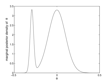
Figure 1: Plot of the marginal posterior density of $\theta$, when the prior density $\pi(\theta,\tau,\sigma^{2})$ is $\big{(}\xi\delta(\tau)+(1-\xi)\big{)}\sigma^{-2}$, $\xi=0.8$, $\rho=0.98$, $m=100$, $\hat{\theta}=0$, $\hat{\sigma}=0.1$ and $\hat{\tau}/\hat{\sigma}=3$.

Define $\ell_{B}(\hat{\theta},\hat{\tau},\hat{\sigma};\eta)$ to be the solution for $\ell$ of $P(\theta<\ell\,|\,\hat{\theta},\hat{\tau},\hat{\sigma})=\eta$, where $P(\,\cdot\,|\,\hat{\theta},\hat{\tau},\hat{\sigma})$ denotes the posterior probability. Also define $u_{B}(\hat{\theta},\hat{\tau},\hat{\sigma};\delta)$ to be the solution for $u$ of $P(\theta>u\,|\,\hat{\theta},\hat{\tau},\hat{\sigma})=\delta$. The Bayesian $1-\alpha$ equi-tailed credible interval is $\big{[}\ell_{B}(\hat{\theta},\hat{\tau},\hat{\sigma};\alpha/2),\,u_{B}(\hat{\theta},\hat{\tau},\hat{\sigma};\alpha/2)\big{]}$. The Bayesian $1-\alpha$ shortest credible interval is $\big{[}\ell_{B}(\hat{\theta},\hat{\tau},\hat{\sigma};\eta^{*}),\,u_{B}(\hat{\theta},\hat{\tau},\hat{\sigma};\alpha-\eta^{*})\big{]}$, where $\eta^{*}$ minimizes the length of the $1-\alpha$ credible interval $\big{[}\ell_{B}(\hat{\theta},\hat{\tau},\hat{\sigma};\eta),\,u_{B}(\hat{\theta},\hat{\tau},\hat{\sigma};\alpha-\eta)\big{]}$ with respect to $\eta\in(0,\alpha)$. Observe that

scaled half-length $$=\frac{1}{2}\left(\frac{u_{B}(\hat{\theta},\hat{\tau},\hat{\sigma};\delta)-\hat{\theta}}{\hat{\sigma}}-\frac{\ell_{B}(\hat{\theta},\hat{\tau},\hat{\sigma};\eta)-\hat{\theta}}{\hat{\sigma}}\right)$$ (5)

scaled offset $$=\frac{1}{2}\left(\frac{u_{B}(\hat{\theta},\hat{\tau},\hat{\sigma};\delta)-\hat{\theta}}{\hat{\sigma}}+\frac{\ell_{B}(\hat{\theta},\hat{\tau},\hat{\sigma};\eta)-\hat{\theta}}{\hat{\sigma}}\right).$$ (6)

Suppose that $\xi\in(0,1)$. As proved in Appendix I, both $\big{(}\ell_{B}(\hat{\theta},\hat{\tau},\hat{\sigma};\eta)-\hat{\theta}\big{)}/\hat{\sigma}$ and $\big{(}u_{B}(\hat{\theta},\hat{\tau},\hat{\sigma};\delta)-\hat{\theta}\big{)}/\hat{\sigma}$ are functions of $(\hat{\sigma},\hat{\tau}/\hat{\sigma})$. It follows from this that the scaled half-length and the scaled offset cannot both be functions of $\hat{\tau}/\hat{\sigma}$. This can be proved by contradiction as follows. Suppose that the scaled half-length and the scaled offset are both functions of $\hat{\tau}/\hat{\sigma}$. The sum and difference of the scaled half-length and the scaled offset must also be functions of $\hat{\tau}/\hat{\sigma}$. This establishes a contradiction.

Also observe that, irrespective of how large $|\hat{\tau}|/\hat{\sigma}$ is, we can find $\hat{\sigma}$ sufficiently small that the Bayesian $1-\alpha$ equi-tailed and shortest credible intervals do not approximate the interval $\big{[}\hat{\theta}-t(m)\hat{\sigma},\,\hat{\theta}+t(m)\hat{\sigma}\big{]}$. By contrast, the interval $J(b,s)$ reverts to the interval $\big{[}\hat{\theta}-t(m)\hat{\sigma},\,\hat{\theta}+t(m)\hat{\sigma}\big{]}$ when $|\hat{\tau}|/\hat{\sigma}\geq d$. In summary: the Bayesian $1-\alpha$ equi-tailed and shortest credible intervals depend on the data in a very different way from this frequentist confidence interval $J(b,s)$.

For further numerical illustration, we consider the following example.

$\boldsymbol{2\times 2}$ factorial experiment example

Consider a $2\times 2$ factorial experiment with 2 replicates and parameter of interest $\theta$ the simple effect (expected response when factor A is high and factor B is low) $-$ (expected response when factor A is low and factor B is low). Suppose that we have uncertain prior information that the two-factor interaction is zero.

Let $x_{1}$ take the values $-1$ and 1 when the factor A takes the values low and high respectively. Also let $x_{2}$ take the values $-1$ and 1 when the factor B takes the values low and high respectively. In other words, $x_{1}$ and $x_{2}$ are the coded values of the factors A and B, respectively. The model for this experiment is

$$Y=\beta_{0}+\beta_{1}x_{1}+\beta_{2}x_{2}+\beta_{12}x_{1}x_{2}+\varepsilon$$

where $Y$ is the response, $\beta_{0}$, $\beta_{1}$, $\beta_{2}$ and $\beta_{12}$ are unknown parameters and the $\varepsilon$ for different response measurements are independent and identically $N(0,\sigma^{2})$ distributed. In this case, $n=8$ and $p=4$, so that $m=n-p=4$. Thus $\theta=2(\beta_{1}-\beta_{12})$. Let $\hat{\beta}_{1}$ and $\hat{\beta}_{12}$ denote the least squares estimators of $\beta_{1}$ and $\beta_{12}$ respectively. The least squares estimator of $\theta$ is $\hat{\theta}=2(\hat{\beta}_{1}-\hat{\beta}_{12})$. Our uncertain prior information is that $\beta_{12}=0$. Note that $\rho=\text{Corr}(\hat{\theta},\hat{\tau})=-1/\sqrt{2}$.

Figures 2 and 3 illustrate the dependence of the scaled offset and scaled half-length on both $\hat{\sigma}$ and $\hat{\tau}/\hat{\sigma}$ for the Bayesian 0.95 equi-tailed and shortest credible intervals for $\theta$, in the context of this $2\times 2$ factorial experiment example, when the prior density $\pi(\theta,\tau,\sigma^{2})$ is $\big{(}\xi\delta(\tau)+(1-\xi)\big{)}\sigma^{-2}$ and $\xi=1/1.2$.

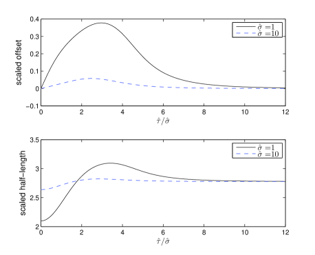
Figure 2: Graphs of the scaled offset and scaled half-length, as functions of $\hat{\tau}/\hat{\sigma}$, for $\hat{\sigma}=1$ (solid line) and $\hat{\sigma}=10$ (dashed line). These are for the Bayesian 0.95 equi-tailed credible interval for $\theta$, in the context of the $2\times 2$ factorial experiment example, when the prior density $\pi(\theta,\tau,\sigma^{2})$ is $\big{(}\xi\delta(\tau)+(1-\xi)\big{)}\sigma^{-2}$ and $\xi=1/1.2$.

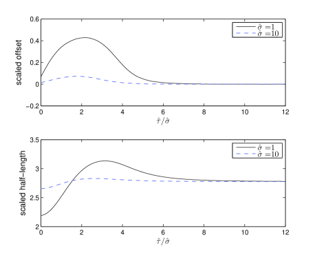
Figure 3: Graphs of the scaled offset and scaled half-length, as functions of $\hat{\tau}/\hat{\sigma}$, for $\hat{\sigma}=1$ (solid line) and $\hat{\sigma}=10$ (dashed line). These are for the Bayesian 0.95 shortest credible interval for $\theta$, in the context of the $2\times 2$ factorial experiment example, when the prior density $\pi(\theta,\tau,\sigma^{2})$ is $\big{(}\xi\delta(\tau)+(1-\xi)\big{)}\sigma^{-2}$ and $\xi=1/1.2$.

4. Bayesian interval estimators for the prior density
$\boldsymbol{\pi(\theta,\tau,\sigma^{2})=\xi\delta(\tau)\sigma^{-1}+(1-\xi)\sigma^{-2}}$

Let $\gamma=\tau/\sigma$. Since we assume that $\sigma>0$, the uncertain prior information that $\tau=0$ can also be expressed as the uncertain prior information that $\gamma=0$. Suppose that, conditional on $\sigma$, $\gamma$ has the improper prior density $\xi\delta(\gamma)+(1-\xi)$, where $\xi\in[0,1]$. Transformations of improper prior densities are problematic. Nonetheless, the plausibility argument presented in Appendix J suggests that this corresponds to $\tau$ having prior density $\xi\delta(\tau)+(1-\xi)\sigma^{-1}$, conditional on $\sigma$. We assume throughout the paper that the prior distributions of $\theta$ and $(\tau,\sigma^{2})$ are independent and that $\theta$ has a uniform prior distribution over the real line. Assuming that $\sigma^{2}$ has the standard noninformative prior density $1/\sigma^{2}$, we obtain the prior density $\pi(\theta,\tau,\sigma^{2})=\xi\delta(\tau)\sigma^{-2}+(1-\xi)\sigma^{-3}$. Interestingly, for this prior density, both the scaled half-length and the scaled offset are functions of $\hat{\tau}/\hat{\sigma}$. In fact, it follows from (5) and (6) and the results derived in Appendix L, that this is true for all prior densities of the form $\pi(\theta,\tau,\sigma^{2})=\xi\delta(\tau){\sigma}^{-g}+(1-\xi){\sigma}^{-g-1}$, where $m+g>0$.

We focus on the particular case that $g=1$, so that the prior density is $\pi(\theta,\tau,\sigma^{2})=\xi\delta(\tau)\sigma^{-1}+(1-\xi)\sigma^{-2}$. We have chosen to focus on this prior density because, for $\xi=0$ i.e. for no prior information about $\tau$, the $1-\alpha$ HPD and equi-tailed credible intervals for $\theta$ are identical to the usual frequentist $1-\alpha$ confidence interval $I$. As shown in Appendix K, the posterior marginal density of $\theta$ is equal to

$$\tilde{\lambda}(\hat{\tau}/\hat{\sigma},1)\,f_{m}(\theta;\mu_{1},\sigma_{1}^{2}(1))+(1-\tilde{\lambda}(\hat{\tau}/\hat{\sigma},1))\,f_{m}(\theta;\hat{\theta},\hat{\sigma}^{2}),$$

where $\mu_{1}=\hat{\theta}-\rho\hat{\tau}$, $\sigma_{1}^{2}(1)=(m\hat{\sigma}^{2}+\hat{\tau}^{2})(1-\rho^{2})/m$,

$$\tilde{\lambda}(\hat{\tau}/\hat{\sigma},1)=\frac{1}{1+\tilde{k}(1)\big{(}m+(\hat{\tau}/\hat{\sigma})^{2}\big{)}^{(m+1)/2}}$$

and

$$\tilde{k}(1)=\frac{\sqrt{2\pi}\,(1-\xi)}{\xi m^{m/2}}.$$

For the case that $\tau$ is known to be 0 (i.e. $\xi=1$), the posterior marginal density for $\theta$ is $f_{m}(\theta;\mu_{1},\sigma_{1}^{2}(1))$, instead of the density $f_{m+1}\big{(}\theta;\mu_{1},\sigma_{1}^{2}(2)\big{)}$ which results from the prior density $\pi(\theta,\tau,\sigma^{2})=\big{(}\xi\delta(\tau)+(1-\xi)\big{)}{\sigma}^{-2}$. Therefore, for this case, the $1-\alpha$ HPD and equi-tailed credible intervals for $\theta$ are not the same as the usual frequentist $1-\alpha$ confidence interval for $\theta$, assuming that $\tau=0$. On the other hand, the $1-\alpha$ credible intervals for $\theta$ based on $f_{m}(\theta;\mu_{1},\sigma_{1}^{2}(1))$ and $f_{m+1}\big{(}\theta;\mu_{1},\sigma_{1}^{2}(2)\big{)}$ are approximately equal for large $m$ in the sense that they are both centered on $\mu_{1}$ and the ratio of their lengths approaches 1, as $m\rightarrow\infty$.

Also observe that $\tilde{\lambda}(\hat{\tau}/\hat{\sigma})\rightarrow 0$ as $|\hat{\tau}|/\hat{\sigma}\rightarrow\infty$. Therefore, the Bayesian $1-\alpha$ equi-tailed and shortest credible intervals approach the interval $\big{[}\hat{\theta}-t(m)\hat{\sigma},\,\hat{\theta}+t(m)\hat{\sigma}\big{]}$ when $|\hat{\tau}|/\hat{\sigma}$ is large. Similarly, the interval $J(b,s)$ reverts to this interval when $|\hat{\tau}|/\hat{\sigma}\geq d$.

Figures 4 and 5 illustrate the fact that the scaled offset and scaled half-length are functions of $\hat{\tau}/\hat{\sigma}$ for the Bayesian 0.95 equi-tailed and shortest credible intervals for $\theta$, in the context of the $2\times 2$ factorial experiment example, when the prior density $\pi(\theta,\tau,\sigma^{2})$ is $\xi\delta(\tau)\sigma^{-1}+(1-\xi)\sigma^{-2}$ and $\xi=1/1.2$.

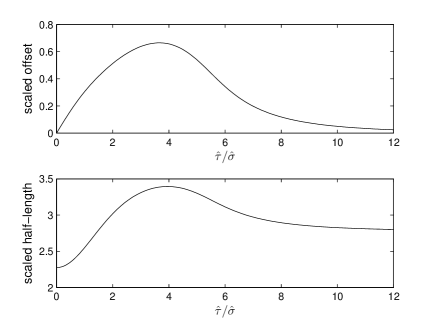
Figure 4: Graphs of the scaled offset and the scaled half-length, as functions of $\hat{\tau}/\hat{\sigma}$, for the Bayesian 0.95 equi-tailed credible interval for $\theta$, in the context of the $2\times 2$ factorial experiment example, when the prior density $\pi(\theta,\tau,\sigma^{2})$ is $\xi\delta(\tau)\sigma^{-1}+(1-\xi)\sigma^{-2}$ and $\xi=1/1.2$.

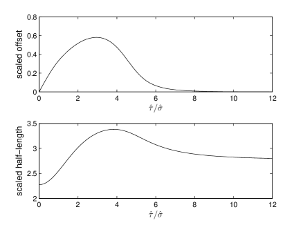
Figure 5: Graphs of the scaled offset and the scaled half-length, as functions of $\hat{\tau}/\hat{\sigma}$, for the Bayesian 0.95 shortest credible interval for $\theta$, in the context of the $2\times 2$ factorial experiment example, when the prior density $\pi(\theta,\tau,\sigma^{2})$ is $\xi\delta(\tau)\sigma^{-1}+(1-\xi)\sigma^{-2}$ and $\xi=1/1.2$.

5. Comparison with the KG $\boldsymbol{1-\alpha}$ confidence interval

We begin this section by briefly describing a method for computing the KG $1-\alpha$ confidence interval for $\theta$ that utilizes the uncertain prior information that $\tau=0$, in the sense described in the introduction. For given $(b,s)$, the coverage probability $P\big{(}\theta\in J(b,s)\big{)}$ is an even function of $\gamma$. The scaled expected length of $J(b,s)$ is (expected length of $J(b,s)$)/(expected length of $I$) and is an even function of $\gamma$ for given $s$, which we denote by $e(\gamma;s)$. Define the weight function $w(\gamma)=\tilde{\xi}\delta(\gamma)+(1-\tilde{\xi})$, where $0\leq\tilde{\xi}\leq 1$. Kabaila and Giri (2009) describe how to compute smooth functions $b$ and $s$ such that (a) the minimum of $P\big{(}\theta\in J(b,s)\big{)}$ over $\gamma$ is $1-\alpha$ and (b)

$$\int_{-\infty}^{\infty}(e(\gamma;s)-1)\,w(\gamma)\,d\gamma$$ (7)

is minimized, where $\tilde{\xi}$ is a specified tuning parameter. This tuning parameter and the functions $b$ and $s$ are chosen by the statistician prior to looking at the observed response vector $\boldsymbol{y}$.

Consider the $2\times 2$ factorial experiment example. For $d=6$, functions $b$ and $s$ chosen to be natural cubic splines in the interval $[0,d]$, with evenly-spaced knots at $0,2,4,\dots,12$, $1-\alpha=0.95$ and $\tilde{\xi}=1/1.2$, the minimization of (7), subject to the coverage constraint, leads to a confidence interval with the following properties. To within computational accuracy, this confidence interval has coverage probability 0.95 for all $\gamma$ (i.e. throughout the parameter space). Figure 6 is a plot of the squared scaled expected length of this confidence interval, as a function of $\gamma$. It is clear from this figure that this confidence interval utilizes the uncertain prior information that $\tau=0$, in the sense described in the introduction. When the prior information is correct (i.e. $\gamma=0$), we gain since $e^{2}(0;s)=0.8524$. The maximum value of $e^{2}(\gamma;s)$ is 1.0852. This confidence interval coincides with the standard $1-\alpha$ confidence interval for $\theta$ when the data strongly contradicts the prior information, so that $e^{2}(\gamma;s)$ approaches 1 as $\gamma\rightarrow\infty$.

Figure 7 shows graphs of the scaled offset and scaled half-length for this confidence interval, as functions of $\hat{\tau}/\hat{\sigma}$. The weight function $w(\gamma)$ has a similar form to the prior density of $\gamma=\tau/\sigma$, conditional on $\sigma$, considered in Section 4, when $\tilde{\xi}=\xi$. Although this weight and conditional prior density have very different interpretations, it is of interest to compare the scaled offset and scaled half-length shown in Figures 4 and 4 with the scaled offset and scaled half-length shown in Figure 7. The differences are marked, particularly with respect to the scaled offset.

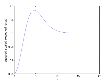
Figure 6: Graph of the squared scaled expected length, as a function of $\gamma$, for the KG 0.95 confidence interval for $\theta$, in the context of the $2\times 2$ factorial experiment example, when $d=12$, $b$ and $s$ are natural cubic splines in the interval $[0,d]$, with evenly-spaced knots at $0,2,4,\dots,12$ and $\tilde{\xi}=1/1.2$.

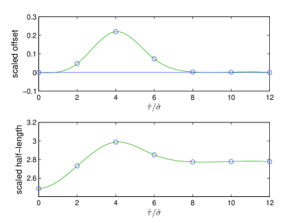
Figure 7: Graphs of the scaled offset and the scaled half-length, as functions of $\hat{\tau}/\hat{\sigma}$, for the KG 0.95 confidence interval for $\theta$, in the context of the $2\times 2$ factorial experiment example, when $d=12$, $b$ and $s$ are natural cubic splines in the interval $[0,d]$, with evenly-spaced knots at $0,2,4,\dots,12$ and $\tilde{\xi}=1/1.2$. The knots of the cubic splines are denoted by small circles.

6. Discussion

We have not sought to advocate the use of Bayesian $1-\alpha$ credible intervals in place of frequentist $1-\alpha$ confidence intervals or vice versa. Bayesian $1-\alpha$ credible intervals could be examined from the point of view of their frequentist coverage properties. Similarly, frequentist $1-\alpha$ confidence intervals could be examined from the point of their Bayesian posterior coverage properties. The first comparison is likely to favor the frequentist $1-\alpha$ confidence intervals, since the Bayesian $1-\alpha$ credible intervals are not constructed to have good frequentist coverage properties. Similarly, the second comparison is likely to favor the Bayesian $1-\alpha$ credible intervals. By contrasting the dependencies on the data of the frequentist $1-\alpha$ confidence intervals and the Bayesian $1-\alpha$ credible intervals, we have avoided a comparison that is partisan to either frequentist or Bayesian points of view.

Bayesian and frequentist statistical analyses differ in important ways. However, it is pleasing when they lead to the same result. In the present paper we have found yet another instance of a difference between Bayesian and frequentist statistical analyses.

Appendix A: Initial scaling of the parameters

We assume that Var$(\hat{\theta})=\sigma^{2}$ and Var$(\hat{\tau})=\sigma^{2}$. In this Appendix, we show that this can be achieved by appropriate scaling and that there is no loss of generality, as far as the purposes of the paper are concerned.

Suppose that the parameter of interest is $\theta^{*}=(\boldsymbol{a}^{*})^{T}\boldsymbol{\beta}$ where $\boldsymbol{a}^{*}$ is a specified $p$-vector ($\boldsymbol{a}^{*}\neq\boldsymbol{0}$). Suppose that the inference of interest is an interval estimator for $\theta^{*}$. Define the parameter $\tau^{*}=(\boldsymbol{c}^{*})^{T}\boldsymbol{\beta}-t^{*}$ where the vector $\boldsymbol{c}^{*}$ and the number $t^{*}$ are specified and $\boldsymbol{a}^{*}$ and $\boldsymbol{c}^{*}$ are linearly independent. Also suppose that previous experience with similar data sets and/or expert opinion and scientific background suggest that $\tau^{*}=0$. In other words, suppose that we have uncertain prior information that $\tau^{*}=0$. Let $v_{11}=(\boldsymbol{a}^{*})^{T}(\boldsymbol{X}^{T}\boldsymbol{X})^{-1}(\boldsymbol{a}^{*})$ and $v_{22}=(\boldsymbol{c}^{*})^{T}(\boldsymbol{X}^{T}\boldsymbol{X})^{-1}(\boldsymbol{c}^{*})$. It is convenient to transform $\theta^{*}$ to $\theta=\theta^{*}/\sqrt{v_{11}}=\boldsymbol{a}^{T}\boldsymbol{\beta}$, where $\boldsymbol{a}=\boldsymbol{a}^{*}/\sqrt{v_{11}}$. It is also convenient to transform $\tau^{*}$ to $\tau=\tau^{*}/\sqrt{v_{22}}=\boldsymbol{c}^{T}\boldsymbol{\beta}-t$, where $\boldsymbol{c}=\boldsymbol{c}^{*}/\sqrt{v_{22}}$ and $t=t^{*}/\sqrt{v_{22}}$. Since $\hat{\theta}=\boldsymbol{a}^{T}\hat{\boldsymbol{\beta}}$ and $\hat{\tau}=\boldsymbol{c}^{T}\hat{\boldsymbol{\beta}}-t$, where $\hat{\boldsymbol{\beta}}\sim N(\boldsymbol{\beta},\sigma^{2}(\boldsymbol{X}^{T}\boldsymbol{X})^{-1})$, Var$(\hat{\theta})=\sigma^{2}$ and Var$(\hat{\tau})=\sigma^{2}$. Interval estimators for $\theta$ and their properties transform in the obvious way to interval estimators for $\theta^{*}$ and their corresponding properties. The uncertain prior information that $\tau^{*}=0$ implies the uncertain prior information that $\tau=0$.

Appendix B: Transformation of the regression model

Define $\boldsymbol{W}=(\boldsymbol{X}^{T}\boldsymbol{X})^{-1}.$ Now define the $p\times p$ matrix $\boldsymbol{B}$ as follows. The first and second rows of $\boldsymbol{B}$ are $\boldsymbol{a}^{T}{\boldsymbol{W}}^{1/2}$ and $\boldsymbol{c}^{T}{\boldsymbol{W}}^{1/2}$, respectively. The last $p-2$ rows consist of unit-length orthogonal $p$ -vectors, that are orthogonal to both $\boldsymbol{a}$ and $\boldsymbol{c}$.

We re-express the regression sampling model as $\boldsymbol{Y}=\tilde{\boldsymbol{X}}\boldsymbol{\lambda}+\boldsymbol{\varepsilon}$, where
$\tilde{\boldsymbol{X}}=\boldsymbol{X}{\boldsymbol{W}}^{1/2}{\boldsymbol{B}}^{-1}$ and $\boldsymbol{\lambda}=\boldsymbol{B}{\boldsymbol{W}}^{-1/2}\boldsymbol{\beta}$. Let $\hat{\boldsymbol{\lambda}}$ denote the least squares estimator of $\boldsymbol{\lambda}$, based on this model. We reduce the data to the sufficient statistic $(\hat{\boldsymbol{\lambda}},\hat{\sigma}^{2})$ for $(\boldsymbol{\lambda},\sigma^{2})$. Let

$$\boldsymbol{V}=\left[\begin{matrix}1\quad\rho\\ \rho\quad 1\end{matrix}\right].$$

Note that $\hat{\boldsymbol{\lambda}}\sim N\big{(}\boldsymbol{\lambda},\sigma^{2}\boldsymbol{D}\big{)}$, where

$$\boldsymbol{D}=\left[\begin{array}[]{c|c}\boldsymbol{V}&\boldsymbol{0}\\ \hline\cr\\[-9.0pt] \boldsymbol{0}&\boldsymbol{I}_{p-2}\\[-1.0pt] \end{array}\right].$$

Observe that $\theta=\lambda_{1}$ and $\tau=\lambda_{2}-t$. Define the parameter vector $\boldsymbol{\chi}=(\lambda_{3},\dots,\lambda_{p})$. Now define $\hat{\boldsymbol{\chi}}=(\hat{\lambda}_{3},\dots,\hat{\lambda}_{p})$. Since $\boldsymbol{D}$ is block diagonal, $(\hat{\theta},\hat{\tau})$ and $\hat{\boldsymbol{\chi}}$ are independent random vectors, $(\hat{\theta},\hat{\tau})$ has the distribution (2) and $\hat{\boldsymbol{\chi}}\sim N\big{(}\boldsymbol{\chi},\sigma^{2}\boldsymbol{I}_{p-2}\big{)}$.

Appendix C: Marginal posterior distribution of $\boldsymbol{(\theta,\tau,\sigma^{2})}$

Suppose that the prior distributions of $(\theta,\tau,\sigma^{2})$ and $\boldsymbol{\chi}$ are independent. Also suppose that the components of $\boldsymbol{\chi}$ have independent uniform prior distributions. In this appendix we prove that the marginal posterior distribution of $(\theta,\tau,\sigma^{2})$ is the same as the posterior distribution of $(\theta,\tau,\sigma^{2})$ based on the reduced data $\big{(}\hat{\theta},\hat{\tau},\hat{\sigma}^{2}\big{)}$ and the sampling model that $\big{(}\hat{\theta},\hat{\tau}\big{)}$ and $\hat{\sigma}^{2}$ are independent random vectors, $\big{(}\hat{\theta},\hat{\tau}\big{)}$ has the distribution (2) and $(n-p)\hat{\sigma}^{2}/\sigma^{2}\sim\chi^{2}_{n-p}$.

It follows from Appendix B that, under the sampling model,

$$f(\hat{\theta},\hat{\tau},\hat{\boldsymbol{\chi}},\hat{\sigma}^{2}|\theta,\tau,\boldsymbol{\psi},\sigma^{2})=f(\hat{\theta},\hat{\tau}|\theta,\tau,\sigma^{2})f(\hat{\boldsymbol{\chi}}|\boldsymbol{\chi},\sigma^{2})f(\hat{\sigma}^{2}|\sigma^{2})$$

where $f(\hat{\boldsymbol{\chi}}|\boldsymbol{\chi},\sigma^{2})=(2\pi\sigma^{2})^{-(p-2)/2}\,\exp\big{(}-{(\hat{\boldsymbol{\chi}}-\boldsymbol{\chi})}^{T}(\hat{\boldsymbol{\chi}}-\boldsymbol{\chi})/2\sigma^{2}\big{)}$.

Suppose that the prior distributions of $(\theta,\tau,\sigma^{2})$ and $\boldsymbol{\chi}$ are independent. Let $\pi(\theta,\tau,\sigma^{2})$ denote the prior density of $(\theta,\tau,\sigma^{2})$. Suppose that the components of $\boldsymbol{\chi}$ are independent and uniformly distributed. Thus the prior density of $(\theta,\tau,\boldsymbol{\chi},\sigma^{2})$ is $\pi(\theta,\tau,\sigma^{2})$. Hence the posterior density $\pi(\theta,\tau,\boldsymbol{\chi},\sigma^{2}|\hat{\theta},\hat{\tau},\hat{\boldsymbol{\chi}},\hat{\sigma}^{2})$ is proportional to $f(\hat{\theta},\hat{\tau}|\theta,\tau,\sigma^{2})f(\hat{\boldsymbol{\chi}}|\boldsymbol{\chi},\sigma^{2})f(\hat{\sigma}^{2}|\sigma^{2})\pi(\theta,\tau,\sigma^{2})$. Thus the marginal posterior density of $(\theta,\tau,\sigma^{2})$ is proportional to

$$f(\hat{\theta},\hat{\tau}|\theta,\tau,\sigma^{2})\boldsymbol{\int}f(\hat{\boldsymbol{\chi}}|\boldsymbol{\chi},\sigma^{2})d\boldsymbol{\chi}\,f(\hat{\sigma}^{2}|\sigma^{2})\,\pi(\theta,\tau,\sigma^{2})=f(\hat{\theta},\hat{\tau}|\theta,\tau,\sigma^{2})f(\hat{\sigma}^{2}|\sigma^{2})\pi(\theta,\tau,\sigma^{2}).$$

Appendix D: Two useful integrals

We make extensive use of the following two integrals:

$$\int_{0}^{\infty}x^{-(p+1)}\,\exp\left(-ax^{-1}\right)\,dx=a^{-p}\,\Gamma(p),$$ (8)

for $a>0$ and $p>0$, which is (A2.1.2) on p.144 of Box and Tiao(1973) and can be proved by a change of variable of integration in the definition of the gamma function, and

$$\int_{-\infty}^{\infty}\exp\left(-\frac{x^{2}-2\rho xy+y^{2}}{2\sigma^{2}(1-\rho^{2})}\right)\,dy=\sqrt{2\pi(1-\rho^{2})}\,\sigma\,\exp\left(-\frac{x^{2}}{2\sigma^{2}}\right)$$ (9)

which can be proved by completion of the square. Note that (9) is used in the derivation of a marginal density for a bivariate normal distribution.

Appendix E: Marginal posterior distribution of $\boldsymbol{\theta}$ for the prior density $\boldsymbol{\pi(\theta,\tau,\sigma^{2})=\delta(\tau)\sigma^{-g}}$

In this appendix we suppose that the prior density is $\pi(\theta,\tau,\sigma^{2})=\delta(\tau){\sigma}^{-g}$, where $m+g>0$. We derive the marginal posterior density of $\theta$. The likelihood function is proportional to $\tilde{\ell}\big{(}\theta,\tau,\sigma^{2}\,|\,\hat{\theta},\hat{\tau},\hat{\sigma}^{2}\big{)}$, which is defined to be

$$\sigma^{-(m+2)}\exp\left(-\frac{m\hat{\sigma}^{2}}{2\sigma^{2}}\right)\exp\left(-\frac{(\theta-\hat{\theta})^{2}-2\rho(\theta-\hat{\theta})(\tau-\hat{\tau})+(\tau-\hat{\tau})^{2}}{2\sigma^{2}(1-\rho^{2})}\right).$$ (10)

Thus the posterior density of $(\theta,\tau,\sigma^{2})$ is proportional to $\tilde{\ell}\big{(}\theta,\tau,\sigma^{2}\,|\,\hat{\theta},\hat{\tau},\hat{\sigma}^{2}\big{)}\delta(\tau){\sigma}^{-g}$, which is equal to

$$\sigma^{-(m+g+2)}\exp\left(-\frac{m\hat{\sigma}^{2}}{2\sigma^{2}}\right)\exp\left(-\frac{(\theta-\hat{\theta})^{2}-2\rho(\theta-\hat{\theta})(\tau-\hat{\tau})+(\tau-\hat{\tau})^{2}}{2\sigma^{2}(1-\rho^{2})}\right)\delta(\tau).$$ (11)

The marginal posterior density of $\theta$ is proportional to

$$\int_{0}^{\infty}\int_{-\infty}^{\infty}\tilde{\ell}\big{(}\theta,\tau,\sigma^{2}\,|\,\hat{\theta},\hat{\tau},\hat{\sigma}^{2}\big{)}\delta(\tau){\sigma}^{-g}\,d\tau\,d\sigma^{2}$$ (12)

which is found as follows. Observe that

$$\int_{-\infty}^{\infty}\exp\left(-\frac{(\theta-\hat{\theta})^{2}-2\rho(\theta-\hat{\theta})(\tau-\hat{\tau})+(\tau-\hat{\tau})^{2}}{2\sigma^{2}(1-\rho^{2})}\right)\delta(\tau)d\tau$$

$$=\exp\left(-\frac{(\theta-\hat{\theta})^{2}+2\rho(\theta-\hat{\theta})\hat{\tau}+\hat{\tau}^{2}}{2\sigma^{2}(1-\rho^{2})}\right)$$

$$=\exp\left(-\frac{\big{(}\theta-(\hat{\theta}-\rho\hat{\tau})\big{)}^{2}}{2\sigma^{2}(1-\rho^{2})}-\frac{\hat{\tau}^{2}}{2\sigma^{2}}\right).$$ (13)

Thus, (12) is equal to

$$\int_{0}^{\infty}\sigma^{-(m+g+2)}\exp\left(-\left(\frac{m\hat{\sigma}^{2}+\hat{\tau}^{2}}{2}+\frac{\big{(}\theta-(\hat{\theta}-\rho\hat{\tau})\big{)}^{2}}{2(1-\rho^{2})}\right){\sigma}^{-2}\right)d\sigma^{2}$$

$$=\Gamma\left(\frac{m+g}{2}\right)\left(\frac{m\hat{\sigma}^{2}+\hat{\tau}^{2}}{2}+\frac{\big{(}\theta-(\hat{\theta}-\rho\hat{\tau})\big{)}^{2}}{2(1-\rho^{2})}\right)^{-(m+g)/2}$$ (14)

by (8). Now (S0.Ex16) can be shown to be equal to $c_{1}(\hat{\tau},\hat{\sigma}^{2},g)f_{m+g-1}(\theta;\mu_{1},{\sigma_{1}}^{2}(g))$, where

$$c_{1}(\hat{\tau},\hat{\sigma}^{2},g)=\sqrt{2\pi(1-\rho^{2})}{\left(\frac{m\hat{\sigma}^{2}+\hat{\tau}^{2}}{2}\right)}^{-(m+g-1)/2}\Gamma\left(\frac{m+g-1}{2}\right)$$ (15)

and $\mu_{1}=\hat{\theta}-\rho\hat{\tau}$ and $\sigma_{1}^{2}(g)=(m\hat{\sigma}^{2}+\hat{\tau}^{2})(1-\rho^{2})/(m+g-1)$. Thus the marginal posterior density of $\theta$ is $f_{m+g-1}(\theta;\mu_{1},{\sigma_{1}}^{2}(g))$, where $f_{q}(\,\cdot\,;\mu,\sigma^{2})$ denotes the density function of $\mu+\sigma T$, where $\sigma>0$ and $T\sim t_{q}$. Note that

$$f_{q}(x;\mu,\sigma^{2})=\frac{1}{\sigma}\,f\left(\frac{x-\mu}{\sigma}\,\bigg{|}\,t_{q}\right),$$

where $f(\,\cdot\,|\,t_{q})$ denotes the $t_{q}$ density function. For the particular case that $g=2$, the marginal prior density of $\theta$ is $f_{m+1}(\theta;\mu_{1},{\sigma_{1}}^{2}(2))$.

Appendix F: Marginal posterior distribution of $\boldsymbol{\theta}$ for the prior density $\boldsymbol{\pi(\theta,\tau,\sigma^{2})=\sigma^{-h}}$

In this appendix we suppose that the prior density is $\pi(\theta,\tau,\sigma^{2})={\sigma}^{-h}$, where $m+h-1>0$. We derive the marginal posterior density of $\theta$. As noted in Appendix E, the likelihood function is proportional to $\tilde{\ell}\big{(}\theta,\tau,\sigma^{2}\,\big{|}\,\hat{\theta},\hat{\tau},\hat{\sigma}^{2}\big{)}$, defined to be (10). Thus the posterior density of $(\theta,\tau,\sigma^{2})$ is proportional to $\tilde{\ell}\big{(}\theta,\tau,\sigma^{2}\,\big{|}\,\hat{\theta},\hat{\tau},\hat{\sigma}^{2}\big{)}{\sigma}^{-h}$, which is equal to

$$\sigma^{-(m+h+2)}\exp\left(-\frac{m\hat{\sigma}^{2}}{2\sigma^{2}}\right)\exp\left(-\frac{(\theta-\hat{\theta})^{2}-2\rho(\theta-\hat{\theta})(\tau-\hat{\tau})+(\tau-\hat{\tau})^{2}}{2\sigma^{2}(1-\rho^{2})}\right).$$ (16)

The marginal posterior density of $\theta$ is proportional to

$$\int_{0}^{\infty}\int_{-\infty}^{\infty}\tilde{\ell}\big{(}\theta,\tau,\sigma^{2}\,|\,\hat{\theta},\hat{\tau},\hat{\sigma}^{2}\big{)}{\sigma}^{-h}\,d\tau\,d\sigma^{2}$$ (17)

which is found as follows. Note that, by (9),

$$\int_{-\infty}^{\infty}\exp\left(-\frac{(\theta-\hat{\theta})^{2}-2\rho(\theta-\hat{\theta})(\tau-\hat{\tau})+(\tau-\hat{\tau})^{2}}{2\sigma^{2}(1-\rho^{2})}\right)d\tau$$

is equal to $\sqrt{2\pi(1-\rho^{2})}\,\sigma\exp\left(-(\theta-\hat{\theta})^{2}/2\sigma^{2}\right)$. Thus (17) is equal to

$$\sqrt{2\pi(1-\rho^{2})}\int_{0}^{\infty}\sigma^{-(m+h+1)}\exp\left(-\left(\frac{m\hat{\sigma}^{2}+(\theta-\hat{\theta})^{2}}{2}\right){\sigma}^{-2}\right)d\sigma^{2}$$

$$=\sqrt{2\pi(1-\rho^{2})}\,\Gamma\left(\frac{m+h-1}{2}\right)\left(\frac{m\hat{\sigma}^{2}+(\theta-\hat{\theta})^{2}}{2}\right)^{-(m+h-1)/2}$$ (18)

by (8). Now (S0.Ex19) is equal to $c_{2}(\hat{\sigma}^{2},h)f_{m+h-2}(\theta;\hat{\theta},{\sigma_{2}}^{2}(h))$, where

$$c_{2}(\hat{\sigma}^{2},h)=2\pi\sqrt{1-\rho^{2}}{\left(\frac{m\hat{\sigma}^{2}}{2}\right)}^{-(m+h-2)/2}\Gamma\left(\frac{m+h-2}{2}\right),$$ (19)

$\sigma_{2}^{2}(h)=(m/(m+h-2))\,\hat{\sigma}^{2}$. Thus the marginal posterior density of $\theta$ is $f_{m+h-2}(\theta;\hat{\theta},{\sigma_{2}}^{2}(h))$ For the particular case that $h=2$, this marginal posterior density is $f_{m}(\theta;\hat{\theta},\hat{\sigma}^{2})$.

Appendix G: An attractive feature of the prior density
$\boldsymbol{\pi(\theta,\tau,\sigma^{2})=\big{(}\xi\delta(\tau)+(1-\xi)\big{)}{\sigma}^{-2}}$

At the end of Appendix E, we considered the extreme case that $\tau$ is known to be 0 i.e. $\pi(\theta,\tau,\sigma^{2})=\delta(\tau)\sigma^{-2}$. This corresponds to choosing $\xi=1$ in the prior density $\pi(\theta,\tau,\sigma^{2})=\big{(}\xi\delta(\tau)+(1-\xi)\big{)}{\sigma}^{-2}$. As shown in this appendix, the marginal posterior density of $\theta$ is $\pi\big{(}\theta\,|\,\hat{\theta},\hat{\tau},\hat{\sigma}^{2}\big{)}=f_{m+1}\big{(}\theta;\mu_{1},\sigma_{1}^{2}(2)\big{)}$, where $\mu_{1}=\hat{\theta}-\rho\hat{\tau}$ and $\sigma_{1}^{2}(2)=(m\hat{\sigma}^{2}+\hat{\tau}^{2})(1-\rho^{2})/(m+1)$. In this case, the HPD and equi-tailed $1-\alpha$ credible intervals for $\theta$ are identical to the usual frequentist $1-\alpha$ confidence interval for $\theta$, assuming that $\tau=0$.

At the end of Appendix F, we considered the second extreme case that there is no prior information about $\tau$ i.e. $\pi(\theta,\tau,\sigma^{2})=\sigma^{-2}$. This corresponds to choosing $\xi=0$ in the prior density $\pi(\theta,\tau,\sigma^{2})=\big{(}\xi\delta(\tau)+(1-\xi)\big{)}{\sigma}^{-2}$. As shown in this appendix, the marginal posterior density of $\theta$ is $\pi(\theta\,|\,\hat{\theta},\hat{\tau},\hat{\sigma}^{2})=f_{m}(\theta;\hat{\theta},\hat{\sigma}^{2})$. In this case also the HPD and equi-tailed $1-\alpha$ credible intervals for $\theta$ are identical and are equal to $\big{[}\hat{\theta}-t(m)\hat{\sigma},\,\hat{\theta}+t(m)\hat{\sigma}\big{]}$. This is the same as the usual frequentist $1-\alpha$ confidence interval for $\theta$, assuming that there is no prior information about $\tau$.

Appendix H: Marginal posterior distribution of $\boldsymbol{\theta}$ for the prior density $\boldsymbol{\pi(\theta,\tau,\sigma^{2})=\big{(}\xi\delta(\tau)+(1-\xi)\big{)}{\sigma}^{-2}}$

Suppose that the prior density is $\pi(\theta,\tau,\sigma^{2})=\big{(}\xi\delta(\tau)+(1-\xi)\big{)}{\sigma}^{-2}$. Also suppose that $\xi\in[0,1]$. The posterior density of $(\theta,\tau,\sigma^{2})$ is proportional to

$$\tilde{\ell}\big{(}\theta,\tau,\sigma^{2}\,\big{|}\,\hat{\theta},\hat{\tau},\hat{\sigma}^{2}\big{)}\big{(}\xi\delta(\tau)+(1-\xi)\big{)}{\sigma}^{-2},$$

where $\tilde{\ell}\big{(}\theta,\tau,\sigma^{2}\,\big{|}\,\hat{\theta},\hat{\tau},\hat{\sigma}^{2}\big{)}$ is defined to be (10). Thus, the marginal posterior density of $\theta$ is proportional to

$$\xi\,\int_{0}^{\infty}\int_{-\infty}^{\infty}\tilde{\ell}\big{(}\theta,\tau,\sigma^{2}\,|\,\hat{\theta},\hat{\tau},\hat{\sigma}^{2}\big{)}\delta(\tau)\,{\sigma}^{-2}\,d\tau\,d\sigma^{2}+(1-\xi)\,\int_{0}^{\infty}\int_{-\infty}^{\infty}\tilde{\ell}\big{(}\theta,\tau,\sigma^{2}\,|\,\hat{\theta},\hat{\tau},\hat{\sigma}^{2}\big{)}\,{\sigma}^{-2}\,d\tau\,d\sigma^{2}.$$

It follows from the derivations presented in Appendices E and F that this is equal to

$$\xi\,c_{1}(\hat{\tau},\hat{\sigma}^{2},2)\,f_{m+1}(\theta;\mu_{1},{\sigma_{1}}^{2}(2))+(1-\xi)\,c_{2}(\hat{\sigma}^{2},2)\,f_{m}(\theta;\hat{\theta},\hat{\sigma}^{2}),$$ (20)

where $\mu_{1}=\hat{\theta}-\rho\hat{\tau}$, $\sigma_{1}^{2}(2)=(m\hat{\sigma}^{2}+\hat{\tau}^{2})(1-\rho^{2})/(m+1)$ and the functions $c_{1}$ and $c_{2}$ are defined by (15) and (19), respectively. Therefore, the marginal posterior density of $\theta$ is

$$\lambda(\hat{\sigma},\hat{\tau}/\hat{\sigma})\,f_{m+1}(\theta;\mu_{1},{\sigma_{1}}^{2}(2))+\left(1-\lambda(\hat{\sigma},\hat{\tau}/\hat{\sigma})\right)\,f_{m}(\theta;\hat{\theta},\hat{\sigma}^{2}),$$

where $\lambda(\hat{\sigma},\hat{\tau}/\hat{\sigma})=\xi\,c_{1}(\hat{\tau},\hat{\sigma}^{2},2)/\left(\xi\,c_{1}(\hat{\tau},\hat{\sigma}^{2},2)+(1-\xi)\,c_{2}(\hat{\sigma}^{2},2)\right)$. Thus

$$\lambda(\hat{\sigma},\hat{\tau}/\hat{\sigma})=\frac{1}{1+k\,\hat{\sigma}\,{\left(m+\big{(}\hat{\tau}/\hat{\sigma}\big{)}^{2}\right)}^{(m+1)/2}},$$

where

$$k=\frac{(1-\xi)\,\sqrt{\pi}\,\,\Gamma(m/2)}{\xi\,m^{m/2}\,\Gamma((m+1)/2)}.$$

Appendix I: Properties of $\boldsymbol{\big{(}\ell_{B}(\hat{\theta},\hat{\tau},\hat{\sigma};\eta)-\hat{\theta}\big{)}/\hat{\sigma}}$ and
$\boldsymbol{\big{(}u_{B}(\hat{\theta},\hat{\tau},\hat{\sigma};\delta)-\hat{\theta}\big{)}/\hat{\sigma}}$ for the prior density
$\boldsymbol{\pi(\theta,\tau,\sigma^{2})=\big{(}\xi\delta(\tau)+(1-\xi)\big{)}{\sigma}^{-2}}$

Suppose that the prior density is $\pi(\theta,\tau,\sigma^{2})=\big{(}\xi\delta(\tau)+(1-\xi)\big{)}{\sigma}^{-2}$ and that $\xi\in(0,1)$. The marginal posterior density of $\theta$ is given by (4). Therefore, $\ell_{B}(\hat{\theta},\hat{\tau},\hat{\sigma};\eta)$ is the solution for $v$ of

$$\int_{-\infty}^{v}\lambda(\hat{\sigma},\hat{\tau}/\hat{\sigma})\,f_{m+1}(\theta;\mu_{1},{\sigma_{1}}^{2}(2))+\left(1-\lambda(\hat{\sigma},\hat{\tau}/\hat{\sigma})\right)\,f_{m}(\theta;\hat{\theta},\hat{\sigma}^{2})\,d\theta=\eta$$

and $u_{B}(\hat{\theta},\hat{\tau},\hat{\sigma};\delta)$ is the solution for $v$ of this equation, but with $\eta$ replaced by $1-\delta$. It follows from this that $\ell_{B}(\hat{\theta},\hat{\tau},\hat{\sigma};\eta)$ is the solution for $v$ of

$$\lambda(\hat{\sigma},\hat{\tau}/\hat{\sigma})\, P\left(-\rho\frac{\hat{\tau}}{\hat{\sigma}}+\sqrt{\frac{(m+(\hat{\tau}/\hat{\sigma})^{2})(1-\rho^{2})}{m+1}}T_{m+1}\leq\frac{v-\hat{\theta}}{\hat{\sigma}}\right)$$

$$+\left(1-\lambda(\hat{\sigma},\hat{\tau}/\hat{\sigma})\right)\,P\left(T_{m}\leq\frac{v-\hat{\theta}}{\hat{\sigma}}\right)=\eta$$

and $u_{B}(\hat{\theta},\hat{\tau},\hat{\sigma};\delta)$ is the solution for $v$ of this equation, but with $\eta$ replaced by $1-\delta$, where $T_{m+1}\sim t_{m+1}$ and $T_{m}\sim t_{m}$. Thus $\big{(}\ell_{B}(\hat{\theta},\hat{\tau},\hat{\sigma};\beta)-\hat{\theta}\big{)}/\hat{\sigma}$ is the solution for $w$ of

$$\lambda(\hat{\sigma},\hat{\tau}/\hat{\sigma})\, P\left(-\rho\frac{\hat{\tau}}{\hat{\sigma}}+\sqrt{\frac{(m+(\hat{\tau}/\hat{\sigma})^{2})(1-\rho^{2})}{m+1}}T_{m+1}\leq w\right)$$

$$+\left(1-\lambda(\hat{\sigma},\hat{\tau}/\hat{\sigma})\right)\,P\left(T_{m}\leq w\right)=\eta$$ (21)

and $\big{(}u_{B}(\hat{\theta},\hat{\tau},\hat{\sigma};\delta)-\hat{\theta}\big{)}/\hat{\sigma}$ is the solution for $w$ of this equation, but with $\eta$ replaced by $1-\delta$. Clearly, (S0.Ex40) can be expressed in the following form

$$\lambda(\hat{\sigma},\hat{\tau}/\hat{\sigma})\,F\left(\frac{w+\rho(\hat{\tau}/\hat{\sigma})}{\sqrt{(m+(\hat{\tau}/\hat{\sigma})^{2})(1-\rho^{2})/(m+1)}}\,\Bigg{|}\,t_{m+1}\right)+\left(1-\lambda(\hat{\sigma},\hat{\tau}/\hat{\sigma})\right)\,F(w\,|\,t_{m})=\eta,$$

where $F(\,\cdot\,|\,t_{q})$ denotes the $t_{q}$ cumulative distribution function. We see from this that both $\big{(}\ell_{B}(\hat{\theta},\hat{\tau},\hat{\sigma};\eta)-\hat{\theta}\big{)}/\hat{\sigma}$ and $\big{(}u_{B}(\hat{\theta},\hat{\tau},\hat{\sigma};\delta)-\hat{\theta}\big{)}/\hat{\sigma}$ are functions of $(\hat{\sigma},\hat{\tau}/\hat{\sigma})$.

Appendix J: Plausibility argument leading to the prior
density $\boldsymbol{\pi(\theta,\tau,\sigma^{2})=\xi\delta(\tau)\sigma^{-2}+(1-\xi)\sigma^{-3}}$

Suppose that, conditional on $\sigma$, $\gamma=\tau/\sigma$ has the improper prior density $\xi\delta(\gamma)+(1-\xi)$, where $\xi\in[0,1]$. The prior probability that $\tau=0$, conditional on $\sigma$, is the same as the prior probability that $\tau/\sigma=0$, conditional on $\sigma$. Thus the prior probability that $\tau=0$, conditional on $\sigma$, is $\xi$. Now consider $0<a<b$. The prior probability that $a\leq\tau/\sigma\leq b$, conditional on $\sigma$, is $(b-a)(1-\xi)$. This implies that the prior probability that $a^{\prime}\leq\tau\leq b^{\prime}$, conditional on $\sigma$, is $(b^{\prime}-a^{\prime})(1-\xi)/\sigma$, where $a^{\prime}=a\sigma$ and $b^{\prime}=b\sigma$. A similar argument applies for $a<b<0$. Therefore, $\tau$ has prior density $\xi\delta(\tau)+(1-\xi)\sigma^{-1}$, conditional on $\sigma$.

Appendix K: Marginal posterior distribution of $\boldsymbol{\theta}$ for the prior density $\boldsymbol{\pi(\theta,\tau,\sigma^{2})=\xi\delta(\tau)\sigma^{-g}+(1-\xi)\sigma^{-g-1}}$

Suppose that the prior density is $\pi(\theta,\tau,\sigma^{2})=\xi\delta(\tau){\sigma}^{-g}+(1-\xi){\sigma}^{-g-1}$, where $m+g>0$. Also suppose that $\xi\in[0,1]$. The posterior density of $(\theta,\tau,\sigma^{2})$ is proportional to

$$\tilde{\ell}\big{(}\theta,\tau,\sigma^{2}\,\big{|}\,\hat{\theta},\hat{\tau},\hat{\sigma}^{2}\big{)}\,\big{(}\xi\delta(\tau){\sigma}^{-g}+(1-\xi){\sigma}^{-g-1}\big{)},$$

where $\tilde{\ell}\big{(}\theta,\tau,\sigma^{2}\,\big{|}\,\hat{\theta},\hat{\tau},\hat{\sigma}^{2}\big{)}$ is defined to be (10). Thus, the marginal posterior density of $\theta$ is proportional to

$$\xi\,\int_{0}^{\infty}\int_{-\infty}^{\infty}\tilde{\ell}\big{(}\theta,\tau,\sigma^{2}\,|\,\hat{\theta},\hat{\tau},\hat{\sigma}^{2}\big{)}\delta(\tau)\,{\sigma}^{-g}\,d\tau\,d\sigma^{2}+(1-\xi)\,\int_{0}^{\infty}\int_{-\infty}^{\infty}\tilde{\ell}\big{(}\theta,\tau,\sigma^{2}\,|\,\hat{\theta},\hat{\tau},\hat{\sigma}^{2}\big{)}\,{\sigma}^{-g-1}\,d\tau\,d\sigma^{2}.$$

It follows from the derivations presented in Appendices E and F that this is equal to

$$\xi\,c_{1}(\hat{\tau},\hat{\sigma}^{2},g)\,f_{m+g-1}(\theta;\mu_{1},{\sigma_{1}}^{2}(g))+(1-\xi)\,c_{2}(\hat{\sigma}^{2},g+1)\,f_{m+g-1}(\theta;\hat{\theta},{\sigma_{2}}^{2}(g+1)),$$

where $\mu_{1}=\hat{\theta}-\rho\hat{\tau}$, $\sigma_{1}^{2}(g)=(m\hat{\sigma}^{2}+\hat{\tau}^{2})(1-\rho^{2})/(m+g-1)$, $c_{1}(\hat{\tau},\hat{\sigma}^{2},g)$ is given by (15) and, in accordance with the definitions at the end of Appendix F,

$$c_{2}(\hat{\sigma}^{2},g+1)=2\pi\sqrt{1-\rho^{2}}{\left(\frac{m\hat{\sigma}^{2}}{2}\right)}^{-(m+g-1)/2}\Gamma\left(\frac{m+g-1}{2}\right),$$

and

$${\sigma_{2}}^{2}(g+1)=\frac{m}{m+g-1}\,\hat{\sigma}^{2}.$$

Therefore, the marginal posterior density of $\theta$ is

$$\tilde{\lambda}(\hat{\tau}/\hat{\sigma},g)\,f_{m+g-1}(\theta;\mu_{1},{\sigma_{1}}^{2}(g))+\left(1-\tilde{\lambda}(\hat{\tau}/\hat{\sigma},g)\right)\,f_{m+g-1}(\theta;\hat{\theta},{\sigma_{2}}^{2}(g+1)),$$ (22)

where $\tilde{\lambda}(\hat{\tau}/\hat{\sigma},g)=\xi\,c_{1}(\hat{\tau},\hat{\sigma}^{2},g)/\left(\xi\,c_{1}(\hat{\tau},\hat{\sigma}^{2},g)+(1-\xi)\,c_{2}(\hat{\sigma}^{2},g+1)\right)$. Thus

$$\tilde{\lambda}(\hat{\tau}/\hat{\sigma},g)=\frac{1}{1+\tilde{k}(g)\,{\left(m+\big{(}\hat{\tau}/\hat{\sigma}\big{)}^{2}\right)}^{(m+g-1)/2}},$$

where

$$\tilde{k}(g)=\frac{\sqrt{2\pi}\,(1-\xi)}{\xi\,m^{(m+g-1)/2}}.$$

Appendix L: Properties of $\boldsymbol{\big{(}\ell_{B}(\hat{\theta},\hat{\tau},\hat{\sigma};\eta)-\hat{\theta}\big{)}/\hat{\sigma}}$ and
$\boldsymbol{\big{(}u_{B}(\hat{\theta},\hat{\tau},\hat{\sigma};\delta)-\hat{\theta}\big{)}/\hat{\sigma}}$ for the prior density
$\boldsymbol{\pi(\theta,\tau,\sigma^{2})=\xi\delta(\tau)\sigma^{-g}+(1-\xi)\sigma^{-g-1}}$

Suppose that the prior density is $\pi(\theta,\tau,\sigma^{2})=\xi\delta(\tau){\sigma}^{-g}+(1-\xi){\sigma}^{-g-1}$, where $m+g>0$. Also suppose that $\xi\in[0,1]$. The marginal posterior density of $\theta$ is given by (22). Therefore, $\ell_{B}(\hat{\theta},\hat{\tau},\hat{\sigma};\eta)$ is the solution for $v$ of

$$\int_{-\infty}^{v}\tilde{\lambda}(\hat{\tau}/\hat{\sigma},g)\,f_{m+g-1}(\theta;\mu_{1},{\sigma_{1}}^{2}(g))+\left(1-\tilde{\lambda}(\hat{\tau}/\hat{\sigma},g)\right)\,f_{m+g-1}(\theta;\hat{\theta},{\sigma_{2}}^{2}(g+1))\,d\theta=\eta$$

and $u_{B}(\hat{\theta},\hat{\tau},\hat{\sigma};\delta)$ is the solution for $v$ of this equation, but with $\eta$ replaced by $1-\delta$. It follows from this that $\ell_{B}(\hat{\theta},\hat{\tau},\hat{\sigma};\beta)$ is the solution for $v$ of

$$\tilde{\lambda}(\hat{\tau}/\hat{\sigma},g)\, P\left(-\rho\frac{\hat{\tau}}{\hat{\sigma}}+\sqrt{\frac{(m+(\hat{\tau}/\hat{\sigma})^{2})(1-\rho^{2})}{m+g-1}}\,T_{m+g-1}\leq\frac{v-\hat{\theta}}{\hat{\sigma}}\right)$$

$$+\left(1-\tilde{\lambda}(\hat{\tau}/\hat{\sigma},g)\right)\,P\left(\sqrt{\frac{m}{m+g-1}}\,T_{m+g-1}\leq\frac{v-\hat{\theta}}{\hat{\sigma}}\right)=\eta$$

and $u_{B}(\hat{\theta},\hat{\tau},\hat{\sigma};\delta)$ is the solution for $v$ of this equation, but with $\eta$ replaced by $1-\delta$, where $T_{m+g-1}\sim t_{m+g-1}$. Thus $\big{(}\ell_{B}(\hat{\theta},\hat{\tau},\hat{\sigma};\eta)-\hat{\theta}\big{)}/\hat{\sigma}$ is the solution for $w$ of

$$\tilde{\lambda}(\hat{\tau}/\hat{\sigma},g)\, P\left(-\rho\frac{\hat{\tau}}{\hat{\sigma}}+\sqrt{\frac{(m+(\hat{\tau}/\hat{\sigma})^{2})(1-\rho^{2})}{m+g-1}}\,T_{m+g-1}\leq w\right)$$

$$+\left(1-\tilde{\lambda}(\hat{\tau}/\hat{\sigma},g)\right)\,P\left(\sqrt{\frac{m}{m+g-1}}\,T_{m+g-1}\leq w\right)=\eta$$

and $\big{(}u_{B}(\hat{\theta},\hat{\tau},\hat{\sigma};\delta)-\hat{\theta}\big{)}/\hat{\sigma}$ is the solution for $w$ of this equation, but with $\eta$ replaced by $1-\delta$. Clearly, this equality can be expressed in the following form

$$\tilde{\lambda}(\hat{\tau}/\hat{\sigma},g)\, F\left(\frac{w+\rho(\hat{\tau}/\hat{\sigma})}{\sqrt{(m+(\hat{\tau}/\hat{\sigma})^{2})(1-\rho^{2})/(m+g-1)}}\,\Bigg{|}\,t_{m+g-1}\right)$$

$$+\left(1-\tilde{\lambda}(\hat{\tau}/\hat{\sigma},g)\right)\,F\left(\sqrt{\frac{m+g-1}{m}}\,w\,\Bigg{|}\,t_{m+g-1}\right)=\eta,$$

where $F(\,\cdot\,|\,t_{q})$ denotes the $t_{q}$ cumulative distribution function. We see from this that both $\big{(}\ell_{B}(\hat{\theta},\hat{\tau},\hat{\sigma};\eta)-\hat{\theta}\big{)}/\hat{\sigma}$ and $\big{(}u_{B}(\hat{\theta},\hat{\tau},\hat{\sigma};\delta)-\hat{\theta}\big{)}/\hat{\sigma}$ are functions of $\hat{\tau}/\hat{\sigma}$.

References

Box, G.E.P., Tiao, G.C., 1973. Bayesian Inference in Statistical Analysis. Wiley, New York.

Chipman, H., George, E.I., McCulloch, R.E. (2001). The Practical Implementation of Bayesian Model Selection (with discussion). IMS Lecture Notes - Monograph Series, 38, 65 - 116.

Farchione, D., Kabaila, P., 2008. Confidence intervals for the normal mean utilizing uncertain prior information. Statistics and Probability Letters 78, 1094–1100.

Ferentinos, K.K., Karakostas, K.X., 2006. More on shortest and equi tails confidence intervals. Communications in Statistics -Theory and Methods 35, 821–829.

Johnstone, I.M., Silverman, B.W., 2004. Needles and straw in haystacks: empirical Bayes estimates of possibly sparse sequences. Annals of Statistics 32, 1594–1649.

Johnstone, I.M., Silverman, B.W., 2005. Bayes selection of wavelet thresholds. Annals of Statistics 33, 1700–1752.

Kabaila, P., 2009. The coverage properties of confidence regions after model selection. International Statistical Review, 77, 405–414.

Kabaila, P., Giri, K., 2009. Confidence intervals in regression utilizing uncertain prior information. Journal of Statistical Planning and Inference 139, 3419–3429.

Kabaila, P., Giri, K., Leeb, H., 2010. Admissibility of the usual confidence interval in linear regression. Electronic Journal of Statistics 4, 300–312.

Kabaila, P., Giri, K., 2013. Further properties of frequentist confidence intervals in regression that utilize uncertain prior information. Australian & New Zealand Journal of Statistics, 55, 259–270.

Miller, A., 2002. Subset Selection in Regression, Second Edition. Chapman & Hall/CRC.

Mitchell, T.J., Beauchamp, J.J., 1988. Bayesian variable selection in linear regression. Journal of the American Statistical Association, 83, 1023–1032.

O’Hara, R.B., Sillanpää, M.J., 2009. A review of Bayesian variable selection methods: what, how and which. Bayesian Analysis 4, 85–118.

Zellner, A., 1986. On assessing prior distributions and Bayesian regression analysis with $g$-prior distributions. Pages 233–243 of Bayesian Inference and Decision Techniques, Essays in Honor of Bruno de Finetti, edited by Prem K. Goel and Arnold Zellner, Elsevier, Amsterdam, The Netherlands.