Modifications of thick-target model: re-acceleration of electron beams by static and stochastic electric fields

Abstract

Context. The collisional thick-target model (CTTM) of the impulsive phase of solar flares, together with the famous CSHKP model, presented for many years a “standard” model, which straightforwardly explained many observational aspects of flares. On the other hand, many critical issues appear when the concept is scrutinised theoretically or with the new generation of hard X-ray (HXR) observations. The famous “electron number problem” or problems related to transport of enormous particle fluxes though the corona represent only two of them. To resolve the discrepancies, several modifications of the CTTM appeared.

Aims. We study two of them based on the global and local re-acceleration of non-thermal electrons by static and stochastic electric fields during their transport from the coronal acceleration site to the thick-target region in the chromosphere. We concentrate on a comparison of the non-thermal electron distribution functions, chromospheric energy deposits, and HXR spectra obtained for both considered modifications with the CTTM itself.

Methods. The results were obtained using a relativistic test-particle approach. We simulated the transport of non-thermal electrons with a power-law spectrum including the influence of scattering, energy losses, magnetic mirroring, and also the effects of the electric fields corresponding to both modifications of the CTTM.

Results. We show that both modifications of the CTTM change the outcome of the chromospheric bombardment in several aspects. The modifications lead to an increase in chromospheric energy deposit, change of its spatial distribution, and a substantial increase in the corresponding HXR spectrum intensity.

Conclusions. The re-acceleration in both models reduces the demands on the efficiency of the primary coronal accelerator, on the electron fluxes transported from the corona downwards, and on the total number of accelerated coronal electrons during flares.

1 Introduction

The CTTM of the impulsive phase of solar flares (Brown, 1971) for many years presented a successful tool not only for interpreting the processes related to the energy deposition and HXR production in the footpoint regions of flare loops, but also for naturally explaining many other observational aspects of flares like the Neupert effect (Dennis & Zarro, 1993), the time correlation of footpoint HXR intensity and intensities of chromospheric lines (Radziszewski et al., 2007, 2011), or the radio signatures of particle transport from the corona towards the chromosphere (Bastian et al., 1998). Nevertheless, especially with the onset of modern HXR observations such as Yohkoh/HXT, RHESSI (Kosugi et al., 1991; Lin et al., 2002), a continuously growing number of discrepancies with the CTTM were beginning to appear. The most striking one is the old standing problem concerning the very high electron fluxes required to explain the observed high HXR footpoint intensities. This problem is particularly acute in the context of the “standard” CSHKP flare model when assuming a single coronal acceleration site (Sturrock, 1968; Kopp & Pneuman, 1976; Shibata, 1996), where enormous numbers of electrons involved in the impulsive phase have to be gathered, accelerated, and then transported to the thick-target region located in the chromosphere (Brown & Melrose, 1977; Brown et al., 2009). Another serious class of problems appears as a consequence of enormous electric currents arising from the transport of high electron fluxes through the corona down to the chromosphere and the inevitable generation of the neutralising return current (van den Oord, 1990; Matthews et al., 1996; Karlický, 2009; Holman, 2012). Also the recent measurements of the vertical extent of chromospheric HXR sources (Battaglia et al., 2012) are inconsistent with the values predicted by the CTTM.

Generally, it is very difficult to explain energy transport by means of electron beams with enormous fluxes from the primary coronal acceleration sites assumed to be located in highly structured coronal current sheets (Shibata & Tanuma, 2001; Bárta et al., 2011a, b) to the thermalisation regions that lie relatively deep in the atmosphere and that produce the observed intensities of footpoint HXR emission in the frame of classical CTTM. Therefore various modifications of the CTTM have been proposed to solve the problems. Fletcher & Hudson (2008) suggest a new mechanism of energy transport from the corona downwards by Alfvén waves, which in the chromosphere accelerate electrons to energies for X-ray emission. Furthermore, Karlický & Kontar (2012) have investigated an electron acceleration in the beam-plasma system. Despite efficient beam energy losses to the thermal plasma, they have found that a noticeable part of the electron population is accelerated by Langmuir waves produced in this system. Thus, the electrons accelerated during the beam propagation downwards to the chromosphere can reduce the beam flux in the beam acceleration site in the corona requested for X-ray emission. Another modification of the CTTM is the local re-acceleration thick-target model (LRTTM) that has been suggested by Brown et al. (2009). The model assumes a primary acceleration of electrons in the corona and their transport along the magnetic field lines downwards to the thick-target region. Here they are subject to secondary local re-acceleration by stochastic electric fields generated in the stochastic current sheet cascades (Turkmani et al., 2005, 2006) excited by random photospheric motions.

Karlický (1995) studied another idea – the global re-acceleration thick-target model (GRTTM). The beam electrons accelerated in the primary coronal acceleration site are on their path from the corona to the chromosphere constantly re-accelerated. Such a re-acceleration is caused by small static electric fields generated by the electric currents originating due to the helicity of the magnetic field lines forming the flare loop (e.g. Gordovskyy & Browning, 2011, 2012; Gordovskyy et al., 2013). The magnitude of the static electric field reaches its maximum in the thick-target region owing to the sharp decrease in electric conductivity in the chromosphere and to the prospective convergence of magnetic field in this region.

In this paper we study the effects of the local and global re-acceleration of beam electrons at locations close to the hard X-ray chromospheric sources. Section 2 describes our approximations of LRTTM and GRTTM and their implementation to a relativistic test-particle code. In Section 3 we compare both modifications with CTTM in terms of electron beam distribution functions, chromospheric energy deposits, and HXR spectra. Modelled HXR spectra are also forward-fitted to obtain beam parameters under the assumption of pure CTTM regardless of any re-acceleration. The results are summarised and discussed in Section 4.

2 Model description

2.1 Beam properties and target atmosphere

The simulations presented in this work start with an injection of an initial electron beam into a closed magnetic loop at its summit point using a test-particle approach (Varady et al., 2010). Physically, the initial beam represents a population of non-thermal electrons generated at the primary acceleration site located in the corona above the flare loop. Our simulations do not treat the primary acceleration itself. The non-thermal electrons are assumed to obey a single power law in energy, so their initial spectrum (in units: electrons cm^-2 s^-1 keV^-1) is

$$F(E,z_{0})=\left\{\begin{array}[]{ll}(\delta_{\mathrm{p}}-2)\frac{\mathcal{F}_{0}}{E_{0}^{2}}\left(\frac{E}{E_{0}}\right)^{-\delta_{\mathrm{p}}}&,\ \ \ \mbox{for}\ \ \ E_{0}\leq E\leq E_{1}\\ 0&,\ \ \ \mbox{for other}\ E\\ \end{array}\right.\ \$$ (3)

(Nagai & Emslie, 1984). The electron flux at the loop top, which corresponds to the column density $z_{0}=0$, is determined by the total energy flux $\mathcal{F}_{\mathrm{0}}$, the low and high-energy cutoffs $E_{0}$, $E_{1}$ and the power-law index $\delta_{\mathrm{p}}$. All the models presented in this work start with the same initial beam parameters $\delta_{\mathrm{p}}=3$, $E_{0}=10$ keV and $E_{1}=400$ keV. For $\mathcal{F}_{\mathrm{0}}$ we use two values $\mathcal{F}_{0}=5\times 10^{9}$ and $10^{11}$ erg cm^-2 s^-1, with the latter only as the CTTM reference flux for a comparison with the models of secondary re-acceleration.

We study two various cases of initial pitch angle distribution. The pitch angle $\vartheta$ determines the angle between the non-thermal electron velocity component parallel to the magnetic field line $\varv_{\parallel}$ and the total electron velocity $\varv$

$$\mu\equiv\cos{\vartheta}=\frac{\varv_{\parallel}}{\varv}\ .$$ (4)

The initial $\mu$-distribution is given by function $M(\mu_{0})$ and must be normalised. The angularly dependent initial electron flux is then

$$F(E,\mu_{0},z_{0})=M(\mu_{0})F(E,z_{0})\ ,\qquad\int_{-1}^{1}M(\mu_{0})\mathrm{d}{\mu_{0}}=1\ .$$ (5)

We consider two extreme cases:

1. a fully focussed beam

   $$M^{\mathrm{FF}}\equiv M(\mu_{0})=\frac{1}{2}\delta(\mu_{0}-\mu_{\mathrm{c}})\ ,$$ (6)

   where $\delta$ is the Dirac function and $\mu_{\mathrm{c}}=\pm 1$; and

2. a semi-uniformly distributed beam

   $$M^{\mathrm{SU}}\equiv M(\mu_{0})=\left\{\begin{array}[]{r@{\quad}l}1,&\mu_{0}\in(-1,-0.5)\cup(0.5,1)\\ 0,&\mu_{0}\in(-0.5,0.5)\ .\\ \end{array}\right.$$ (7)

The initial pitch angle distribution reflects the properties of the primary coronal accelerator. The first distribution may represent an extreme case of an electron beam accelerated in the coronal current sheet with an X-point, and the second is close to the outcome of the acceleration mechanisms involving the plasma wave turbulence in a second-order Fermi process (Winter et al., 2011). The electrons with negative $\mu_{0}$ propagate to the left, with positive $\mu_{0}$ to the right half of the loop. Since we study the effects of the electron beam bombardment of the chromosphere, we excluded the population with $\mu_{0}\in(-0.5,0.5)$ from the uniform distribution. This approximation substantially decreases the computational cost. The choice of $M(\mu_{0})$ influences the initial energy flux along magnetic field lines towards a single left or right footpoint. The parallel fluxes towards individual footpoints are $\mathcal{F}_{0}/2$ for $M^{\mathrm{FF}}$ and $3\mathcal{F}_{0}/8$ for $M^{\mathrm{SU}}$, respectively. The total number of non-thermal electrons injected into the loop per unit area and time is $\approx$1.6$\times 10^{17}$ electrons cm^-2 s^-1 (relevant to the energy flux $\mathcal{F}_{0}=5\times 10^{9}$ erg cm^-2 s^-1 and both pitch angle distributions).

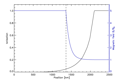
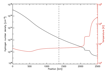
Figure 1: Left: Hydrogen ionisation (black line) and relative magnetic field strength $B/B_{\mathrm{0}}$ (blue line), right temperature (red line), and hydrogen density (black line) in the lower parts of the VAL C atmosphere. The dashed line indicates the lower boundary of the magnetic mirror.

We consider a converging magnetic field along the loop towards the photosphere with a constant mirror ratio $R_{\mathrm{m}}\equiv B_{1}/B_{0}=5$, where $B_{0}$ and $B_{1}$ are the magnetic fields at the loop top in the corona and at the base of the loop in the photosphere, respectively. To model the field convergence we adopted the formula proposed by Bai (1982), where the magnetic field strength $B$ is only a function of the column density $z$ calculated from the loop top downwards

$$\frac{B(z)}{B_{\mathrm{0}}}=\left\{\begin{array}[]{ll}1+(R_{\mathrm{m}}-1)(z/z_{\mathrm{m}})^{2}&,\ \ \ \mbox{for}\ \ \ z\leq z_{\mathrm{m}}\\ R_{\mathrm{m}}&,\ \ \ \mbox{for}\ \ \ z\geq z_{\mathrm{m}}\\ \end{array}\right.\ \ ,$$ (10)

where $z_{\mathrm{m}}=4\times 10^{19}$ cm^-2. For the VAL C atmosphere (Vernazza et al., 1981) $z_{\mathrm{m}}$ is located in the chromosphere – corresponding position $s_{\mathrm{m}}=1.36$ Mm, temperature $T_{\mathrm{m}}=6270$ K and density $n_{\mathrm{m}}=2\times 10^{12}$ cm^-3. The adopted configuration of the magnetic field is shown in Fig. 1. The convergence of the magnetic field in the vicinity of the loop footpoints influences the model in two aspects. First, only part of the beam electrons with low pitch angles satisfying the condition $\sin^{2}\vartheta\leq\frac{1}{R_{\mathrm{m}}}$ passes through the magnetic mirror. Second, the corresponding flux is focussed thanks to the field convergence that results in an increase in the energy deposit per unit volume in the constricted flux tube. The remaining beam particles are reflected by the mirror and move back to the loop top and further to the second part of the loop (Karlický & Henoux, 1993).

The corresponding energy deposits, non-thermal electron distribution functions, and the HXR spectra are determined primarily by the parameters of the electron beam itself, but also by the properties of the target atmosphere. The results are obtained for the VAL C atmosphere (see Fig. 1) (Vernazza et al., 1981), which was extrapolated to the hot $\sim$1 MK and low density $10^{8}$ – $10^{9}$ cm^-3 corona. The length of the whole loop is $L=20$ Mm, so the source of the energetic particles (primary coronal acceleration site) is located at $s=10$ Mm.

The hydrodynamic flare models show that a rapid and massive flare energy release in the thick-target region dramatically changes the temperature and ionisation structure in the chromosphere on very short timescales $\leq 1$ s (Abbett & Hawley, 1999; Allred et al., 2005; Kašparová et al., 2009). Therefore it also influences the thermalisation rate of the non-thermal electrons (Emslie, 1978; Kašparová et al., 2009) and thus the outcome of the bombardment (Varady et al., 2013). Using a hydrodynamic flare code combined with a test-particle code (Varady et al., 2010), we tested the influence in increased temperature and change of ionisation due to the flare heating on the HXR spectra produced in the thick-target region and on the corresponding energy deposits. We found only relatively minor changes in comparison with the results for the quiet VAL C atmosphere. Therefore only results for the quiet VAL C atmosphere are presented in this study.

2.2 Test-particle approach

The problem of collisional particle transport in a partially ionised atmosphere in the cold target approximation was analysed by Emslie (1978). Bai (1982) presented a Monte-Carlo method that is useful for computer implementation of the transport of energetic electrons in a fully ionised hydrogen plasma in a non-uniform magnetic field. It has been shown by MacKinnon & Craig (1991) that the coupled system of stochastic equations presented in Bai (1982) is formally equivalent to the corresponding Fokker-Planck (FP) equation, therefore the method proposed by Bai (1982) has to give equivalent results as the direct solution of the FP equation. We modified the approach of Bai (1982) for a partially ionised cold target and developed a relativistic test-particle code. The code follows the motion of a chain of beam electron clusters, test-particles with a power-law spectrum along a magnetic field line described with the following equation of motion

$$\frac{\mathrm{d}\@vec{p}_{\mathrm{e}}}{\mathrm{d}t}=-{\@vec{C}}_{\mathrm{e}}(\varv_{\mathrm{e}})+{\@vec{F}}_{\mathrm{m}}-e{\@vec{E}}\ ,$$ (11)

where $\@vec{p}_{\mathrm{e}}$ is the momentum of the electron cluster, $-\@vec{C}_{\mathrm{e}}(\varv_{\mathrm{e}})$ is the collisional drag also responsible for the effects of scattering, $\@vec{F}_{\mathrm{m}}$ is the magnetic mirror force, and the term $-e\@vec{E}$ expresses the force controlling the secondary acceleration.

2.3 Collisional thick-target model – CTTM

In the scenario of classical CTTM, the non-thermal electrons lose their energy and are scattered by the Coulomb collisions with the particles of the ambient plasma (see the term $-\@vec{C}_{\mathrm{e}}(\varv_{\mathrm{e}})$ in equation (11)). The energy loss of a non-thermal electron $\Delta E$ with kinetic energy $E$ and velocity $\varv$ caused by Coulomb collisions in a partly ionised hydrogen cold target, per time-step $\Delta t$, can be approximated by

$$\Delta E=-\frac{2\pi e^{4}}{E}\left[\Lambda x+\Lambda^{\prime}(1-x)\right]n\,\varv\,\Delta t\ ,$$ (12)

where $n=n_{\mathrm{p}}+n_{\mathrm{n}}$ is the number density of equivalent hydrogen atoms, $n_{\mathrm{p}}$ and $n_{\mathrm{n}}$ are the proton and hydrogen number densities, respectively, $x=n_{\mathrm{p}}/n$ is the hydrogen ionisation, and $\Lambda$, $\Lambda^{\prime}$ are the Coulomb logarithms (Emslie, 1978).

The scattering due to Coulomb collisions is simulated using the Monte Carlo method. According to Bai (1982), the relation between the rms of the scattering angle $\Delta\vartheta_{\mathrm{C}}$, the ratio $\Delta E/E$, and the Lorentz factor $\gamma_{\mathrm{L}}$ is

$$\overline{\Delta\vartheta_{\mathrm{C}}^{2}}=\left(\frac{\Delta E}{E}\right)\left(\frac{4}{\gamma_{\mathrm{L}}+1}\right)\ ,$$ (13)

when $\overline{\Delta\vartheta_{\mathrm{C}}^{2}}\ll 1$ (or equivalently, $\Delta E/E\ll 1$). The value of scattering angle $\Delta\vartheta_{\mathrm{C}}$ is given by a Gaussian distribution, the rms of which is computed by the equation (13).

The change in the pitch angle caused by the magnetic force $\@vec{F}_{\mathrm{m}}$, see equation (11), in the region of magnetic field convergence is

$$\Delta\vartheta_{\mathrm{B}}=\frac{B_{i+1}-B_{i}}{2B_{i}}\tan{\vartheta_{i}}\ ,$$ (14)

providing $(\Delta\vartheta_{\mathrm{B}})^{2}\ll 1$ in a single time-step, where $B_{i}$ and $B_{i+1}$ are the magnetic field strengths at the beginning and end of the particle path, and $\vartheta_{i}$ is the initial pitch angle. The total change of the pitch angle in a single time-step due to collisions and magnetic field non-uniformity is $\Delta\vartheta=\Delta\vartheta_{\mathrm{C}}+\Delta\vartheta_{\mathrm{B}}$, and the new electron pitch angle $\vartheta$ is then obtained using the cosine rule from the spherical trigonometry

$$\cos\vartheta=\cos\vartheta_{i}\cos\Delta\vartheta+\sin\vartheta_{i}\sin\Delta\vartheta\cos\varphi\ ,$$ (15)

where $\varphi$ is the azimuthal angle given by a uniform distribution $0\leq\varphi<2\pi$. More details concerning computer implementation can be found in Varady et al. (2005, 2010) and Kašparová et al. (2009).

2.4 Secondary accelerating mechanisms

To include the secondary acceleration mechanisms, we added either the static or stochastic electric fields that re-accelerate or decelerate the test-particles with respect to the mutual directions of the electric field and instantaneous test-particle velocities. The interaction of the non-thermal particles with the re-accelerating electric field, the $-e\@vec{E}$ term in equation (11), is calculated using the Boris relativistic algorithm (see Peratt, 1992, Sect. 8.5.2). The effects of the return current are not considered. Relatively low electron fluxes transported from the corona ($\mathcal{F}_{0}/2=2.5\times 10^{9}$ erg cm^-2 s^-1 towards each footpoint) partially justify this negligence.

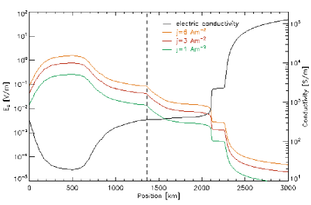
Figure 2: Classical electric conductivity $\sigma$ in the lower VAL C atmosphere according to Kubát & Karlický (1986) and the magnitude of the corresponding ${\bf E}_{\mathrm{G}}$ for various current densities ${\bf j}$.

2.4.1 Static electric field – GRTTM

We now consider a situation where electric currents flow in the flare loop before and during the flare impulsive phase due to the non-zero helicity of the pre-flare magnetic field (Karlický, 1995). Furthermore, at the very beginning of the flare, the current-carrying loops are unstable to the kink and tearing-mode instabilities, which produce filamented electric currents in a natural way (Kuijpers et al., 1981; Karlický & Kliem, 2010; Kliem et al., 2010; Gordovskyy & Browning, 2011). If electrons are accelerated in the coronal part of the individual current thread, they propagate along it and interact with the corresponding global re-acceleration resistive static electric field ${\bf E}_{\mathrm{G}}$ driving the current. The field corresponding to the current density ${\bf j}$ is

$${\bf E}_{\mathrm{G}}={\bf j}/\sigma\ ,$$ (16)

where $\sigma$ is the plasma electric conductivity. The general formula for plasma conductivity is

$$\sigma=\frac{\omega_{\mathrm{pe}}^{2}}{4\pi\nu_{\mathrm{e}}}\ ,$$ (17)

where $\omega^{2}_{\mathrm{pe}}=4\pi e^{2}n_{\mathrm{e}}/m_{\mathrm{e}}$ is the electron plasma frequency, and $\nu_{\mathrm{e}}$ the electron collisional rate. In case electric currents propagate in plasma free of any plasma waves, the collisional frequency corresponds to the classical value

$$\nu_{\mathrm{e}}=2.91\times{10^{-6}}\frac{n_{\mathrm{e}}}{T_{\mathrm{e}}^{3/2}}\ {\Lambda}\ ,$$ (18)

in the SI units, where $T_{\mathrm{e}}$ is the electron temperature. On the other hand, the presence of plasma waves can increase the collisional frequency to anomalous values: for the anomalous resistivity see Heyvaerts (1981).

To assess the influence of static electric field on the outcome of the chromospheric bombardment by non-thermal electrons, we assume a single thread of constant current density with magnitude below any current instability thresholds. Then we calculate the magnitude of corresponding direct field ${\bf E}_{\mathrm{G}}$ along the thread using the classical isotropic electric conductivity obtained by Kubát & Karlický (1986). The conductivity was calculated using the updated values of proton–hydrogen scattering cross-section for the quiet VAL C atmosphere (see Fig. 2). Owing to temperature dependence of $\sigma$ and the convergence of magnetic field in the chromosphere, contributing to the increase in the local current density, the resulting ${\bf E}_{\mathrm{G}}$ grows rather quickly in the chromosphere (see Fig. 2). Furthermore, ${\bf E}_{\mathrm{G}}$ tends to accelerate the beam electrons towards one footpoint and to decelerate them towards the second one, providing an asymmetric flare heating of the individual thread footpoints. From now on, we refer to the individual footpoints as the primary and the secondary footpoints, respectively and to this model as the global re-accelerating thick-target model (GRTTM).

The steep increase in ${\bf E}_{\mathrm{G}}$, hence the high efficiency of GRTTM, is essentially linked with the decrease in temperature in the chromosphere. In contrast, we have already pointed out that chromospheric plasma in flares is heated to temperatures up to $10^{5}$ K on the timescales $\leq 1$ s. Such an extreme increase in temperature substantially increases the classical electric conductivity ($\sigma\propto T_{\mathrm{e}}^{3/2}$) in the corresponding region, and by the same factor it decreases the electric field ${\bf E}_{\mathrm{G}}$, so the flare heating of the chromosphere should basically cease the re-acceleration in the thick-target region very early after the start of the impulsive phase. On the other hand, under the flare conditions, generation of a high anomalous resistivity could be expected due to plasma instabilities, so the accelerating mechanism could continue working.

2.4.2 Stochastic electric fields – LRTTM

Inspired by Brown et al. (2009) and Turkmani & Brown (2012), we produced a simplified local re-acceleration thick-target model (LRTTM). To approximate the distribution of electric fields arising as a consequence of a current sheet cascade in the randomly stressed magnetic fields (Turkmani et al., 2005, 2006), we assume a region (between 1 – 2 Mm) of stochastic re-acceleration electric field ${{\bf E}_{\mathrm{L}}}$, spatially modulated by the function shown in Fig. 3 (bottom). The position of the local re-acceleration region is one of the free parameters of the model. It roughly corresponds to the chromosphere and encompasses the regions of magnetic field convergence and the rapid change of hydrogen ionisation (see Fig. 1).

The stochastic electric fields ${{\bf E}_{\mathrm{L}}}$ are generated only in the directions parallel and anti-parallel relative to the loop axis, and their distribution corresponds to Gaussians with various mean values $\overline{E_{\mathrm{L}}}$ and variances $\mbox{var}(E_{\mathrm{L}})=\overline{E_{\mathrm{L}}^{2}}-\overline{E_{\mathrm{L}}}^{2}.$ We examine two types of ${{\bf E}_{\mathrm{L}}}$:

1. A stochastic electric field with zero mean value

   $$\overline{E_{\mathrm{L}}}=0\ ,\ \ \ \ \ \ \mbox{var}({E_{\mathrm{L}}})>0\ .$$ (19)

2. A combination of spatially localised static electric field with a stochastic component (see Fig. 3)

   $$\overline{E_{\mathrm{L}}}\neq 0\ ,\ \ \ \ \ \mbox{var}{(E_{\mathrm{L}}})\geq 0\ .$$ (20)

In the case of ${{\bf E}_{\mathrm{L}}}$-II, the sign of the static component $\overline{E_{\mathrm{L}}}$ always assures acceleration of the non-thermal electrons towards the nearest footpoint. This field type can develop in the thick-target region if stochastic fields are present in a globally twisted magnetic loop. In comparison with the GRTTM, the LRTTM is characterised by abrupt changes in magnitude and orientation of the accelerating or decelerating electric fields representing the individual current sheets in the thick-target region (Turkmani et al., 2006) (compare Figs. 2 and 3).

The integration of motion of individual beam electron clusters for the LRTTM is performed in the following way. In each time-step (corresponding to $\Delta t=5\times 10^{-5}$ s), we generate a random value of ${\bf E}_{\mathrm{L}}$ for each particle within the acceleration region. In this way we model the situation where the beam electrons are moving in the stochastic electric fields, whose configuration temporally changes. Therefore, the electrons only have a negligible chance of passing through exactly the same configuration of current sheets and of experiencing the same acceleration (deceleration) sequence. The time-step basically determines the spatial extent of the individual current sheets. In order to keep the size independent of particle velocities, we weight ${\bf E}_{\mathrm{L}}$ using a factor $\varv_{0}/\varv$, where $\varv_{0}$ and $\varv$ are the velocities corresponding to the low-energy cutoff and to the particular particle, respectively. The time-step $\Delta t=5\times 10^{-5}$ s thus corresponds to the current sheet size $\sim$3 km. Simulations with various time-steps showed that the results are not very sensitive to the choice of the time-step. Using the weighted value of ${\bf E}_{\mathrm{L}}$ we relativistically move the electron from the old to the new position. Then we calculate the energy loss and scattering due to the passage of the particle through the corresponding column of plasma and the effects of converging magnetic field. This is done repeatedly for the whole population of test-particles. The corresponding total energy deposit and HXR spectrum are then calculated.

Figure 3: Top: Example of ${{\bf E}_{\mathrm{L}}}$-II type stochastic electric field with $\overline{E_{\mathrm{L}}}=0.1$ V m^-1 and $\mbox{var}(E_{\mathrm{L}})=0.5$ V m^-1 corresponding to the distribution function in Fig. 13. Bottom: The the spatial modulation of ${\bf E}_{\mathrm{L}}$.

2.5 HXR spectra

The intensity $I(\epsilon,s)$ [photons cm^-2 s^-1 keV^-1] of HXR bremsstrahlung observed on energy $\epsilon$, emitted by plasma at a position $s$ along the flare loop, detected in the vicinity of the Earth, was calculated using the formula (Brown, 1971)

$$I(\epsilon,s)=\frac{n_{\mathrm{p}}(s)V(s)}{4\pi R^{2}}\int_{\epsilon}^{\infty}Q(E,\epsilon)\;\varv(E)\;n(E,s)\,\mathrm{d}E\ .$$ (21)

Here, $n_{\mathrm{p}}(s)V(s)$ is the total number of protons in the emitting plasma volume $V(s)$ at a position $s$, distance $R=1$ AU, $\varv(E)$ is the electron velocity calculated relativistically from the electron energy, and $n(E,s)$ is the number density of non-thermal electrons per energy in the emitting volume having kinetic energy $E$. The cross section $Q(E,\epsilon)$ for bremsstrahlung was calculated using a semi-relativistic formula given by (Haug, 1997), multiplied by the Elwert factor (Elwert, 1939), considering the limit case when the entire electron kinetic energy is emitted. The precision of the method should be better than 1 % for energies $\leq 300$ keV (Haug, 1997). To calculate the emitting volume $V(s)$ we assume a circular cross section of the converging loop with a radius $r(s)=1.5\sqrt{B_{\mathrm{0}}/B(s)}$ Mm. The HXR spectra are calculated on a spatial (height) grid $(s,s+\Delta s)$. The individual emitting volumes along the grid are then $V(s)=\pi r(s)^{2}\Delta s$.

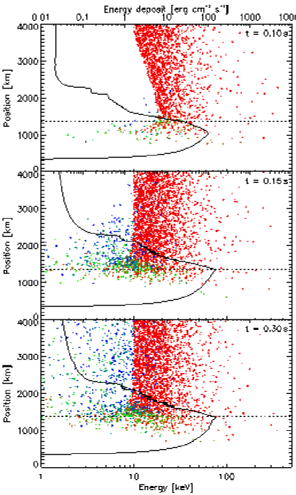
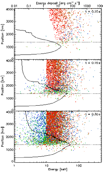
Figure 4: CTTM time evolution of distribution functions of non-thermal electron energies versus positions with a colour coded $M(\mu_{0})$ in the VAL C atmosphere. Left: $M^{\mathrm{FF}}$, right: $M^{\mathrm{SU}}$. From top to bottom: individual snapshots at $t=0.1,0.15,0.3$ s after the beam injection into the loop at its apex. The solid lines indicate the instantaneous energy deposits corresponding to ${\mathcal{F}}_{\mathrm{0}}/2=2.5\times 10^{9}$ erg cm^-2 s^-1. The dotted horizontal lines indicate the bottom boundary of the magnetic mirror. Only the lower part of the loop and one footpoint are displayed.

3 Results

We now concentrate on a comparison of outcomes of chromospheric bombardment for two modifications of CTTM with the CTTM itself. In this section we present the non-thermal electron distribution functions in the vicinity of footpoints and several properties of the corresponding energy deposits and HXR intensities and spectra. The quantitative results for the CTTM, GRTTM, and both considered types of LRTTM are summarised in Figs. 8, 11, and 12 and Tables 1, 2, and 3, respectively (Tables 2 and 3 available only in the online version). Here, the factor $\mathcal{F_{\mathrm{R}}}/\mathcal{F}_{\mathrm{0}}$ gives the ratio of the reflected (due to the magnetic mirroring, re-acceleration, and backscattering) to the original non-thermal electron energy flux coming from the corona at position $s=3$ Mm, measured at $t=0.3$ s after the beam injection into the loop at its apex. To assess the magnitude of the energy deposits for the individual models, we calculate the total energy deposited into the chromosphere along a magnetic flux tube as

$$\mathcal{E}_{\mathrm{ch}}=\int\limits_{\mathrm{chromosphere}}{E_{\mathrm{dep}}(s)}\mathrm{d}{V(s)}=S_{0}B_{0}\int\limits_{0}^{2.3\mathrm{Mm}}\frac{E_{\mathrm{dep}}(s)}{B(s)}\mathrm{d}{s}\$$ (22)

and give the position of the energy deposit maximum $s_{\max}$ in the atmosphere. The factor $B_{0}/B(s)$ in integral (22) accounts for the convergence of the magnetic field, $E_{\mathrm{dep}}(s)$ is the local energy deposit in units [erg cm^-3 s^-1], and the limits of integration correspond to the upper and lower boundaries of the chromosphere. The lower limit lies far below the stopping depths of the beam electrons for all the studied models. When all the beam energy is deposited into the chromosphere and $S_{0}=1$ cm², the value of $\mathcal{E}_{\mathrm{ch}}$ in units [erg s^-1] corresponds to the value of the initial flux $\mathcal{F}_{\mathrm{0}}$.

For HXR we give the intensity $I_{25\,\mathrm{keV}}$ and the power-law index $\gamma_{25\,\mathrm{keV}}$ measured at energy 25 keV. Furthermore, we applied the RHESSI spectral analysis software (OSPEX) to modelled total X-ray spectra to imitate common spectral analysis. We assumed that these spectra were incident on RHESSI detectors and forward-fitted the “detected” count spectra. In the fitting we used the OSPEX thick-target model and a single power-law injected electron spectrum. In this way we obtained the fitted electron beam parameters. To account for the non-uniform ionisation structure of the X-ray emitting atmosphere, the fitting function f_thick_nui in the step-function mode was chosen. When the fitted parameters of f_thick_nui were unrealistic and the X-ray emission was formed deep in the layers of almost neutral plasma, f_thick with neutral energy loss term was used. Also, we modified the standard OSPEX energy loss term and the ratio of Coulomb logarithms to be consistent with relations used in the test-particle code. The results of this analysis, the fitted energy flux $\mathcal{F}_{\mathrm{0}}^{\prime}$, the power-law index $\delta_{\mathrm{p}}^{\prime}$, and the low-energy cutoff $E_{0}^{\prime}$ are listed in Tables 1, 2, and 3 and displayed in Figs. 8, 11, and 12.

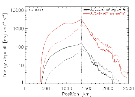
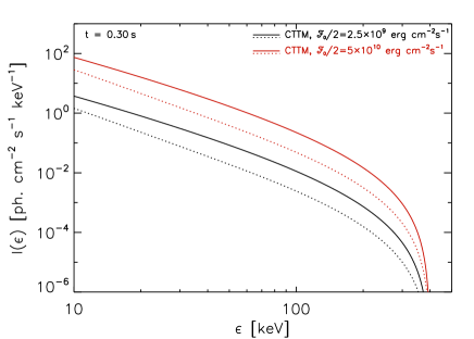
Figure 5: Left: CTTM instantaneous energy deposits into the VAL C atmosphere at $t$=0.3 s for energy fluxes $\mathcal{F}_{\mathrm{0}}/2=5\times 10^{10}$ erg cm^-2 s^-1 (red lines) and $\mathcal{F}_{\mathrm{0}}/2=2.5\times 10^{9}$ erg cm^-2 s^-1 (black lines). The dotted vertical line indicates the bottom boundary of the magnetic mirror. Right: The HXR spectra integrated over one half of the loop. In both panels the solid lines represent $M^{\mathrm{FF}}$, the dotted lines $M^{\mathrm{SU}}$ case.

3.1 CTTM

To produce a basis for comparison we present results for the classical CTTM in a converging magnetic field. The information on kinematics of non-thermal electrons for both initial $\mu$-distributions we considered is incorporated into Fig. 4. We first concentrate on the left-hands panels showing the time dependent distributions for $M^{\mathrm{FF}}$ case. The top panel for $t=0.1$ s corresponds to the transition state when the loop is being filled with non-thermal electrons. The process of filling is apparent as a depletion of the distribution function at low energies in the region ranging from approximately $1.4$ Mm to $3.7$ Mm. The distribution above the low-energy cutoff and the bottom boundary of the magnetic mirror is dominated by red, so a vast majority of particles move downwards with $\mu\approx 1$. At low energies ($E<20$ keV), a low-energy tail of particles starts to form in the region under the lower boundary of the magnetic mirror. It consists of particles with originally higher energies that lost part of their energy owing to their interactions with the target plasma. The tail is rich in particles with $\mu\approx 0$ (green), and it also contains a few back-scattered particles with $\mu\approx-1$ (blue). Coulomb scattering leads to an increase in pitch angles of low-energy electrons in the region above the magnetic mirror. These particles do not satisfy the condition for passing through the mirror. They are reflected and propagate back to the loop top and fill the loop with a population of low-energy electrons ($<20$ keV) with $-1\leq\mu<0$.

Such a low-energy tail is more clearly pronounced in the subsequent times in the vicinity and slightly above the lower boundary of the magnetic mirror. The following snapshot for $t=0.15$ s, when even the particles with lowest energies reached the thick-target region, shows the proceeding thermalisation of beam electrons in this region and increase in particle number with $\mu\leq 0$ in the low-energy tail. A new population of particles with $\mu\approx-1$ starts to form and propagate upwards, towards the loop top. The snapshot at $t=0.3$ s roughly corresponds to a fully developed state. The part of the distribution function at the vicinity of the bottom boundary of the magnetic mirror and in the low-energy region $E<20$ keV is dominated by particles with $\mu\approx 0$. The reflected energy flux propagating upwards is approximately 4% of the original flux $\mathcal{F}_{\mathrm{0}}$ for the $M^{\mathrm{FF}}$ case (see Table 1).

The distribution functions corresponding to $M^{\mathrm{SU}}$ are shown in Fig. 4 (right). The overall behaviour of the beam electrons is quite similar to the previously discussed case. The most obvious difference is the enhancement of the particle populations with $\mu<0$ on all energies (corresponding to 40% of the initial flux $\mathcal{F}_{\mathrm{0}}$) and $\mu\approx 0$ predominantly on low energies ($E<40$ keV) localised above the bottom boundary of the magnetic mirror. The differences between the $M^{\mathrm{FF}}$ and $M^{\mathrm{SU}}$ cases naturally influence the resulting energy deposits and properties of the corresponding HXR emission (see Figs. 4, 5). The CTTM in the adopted arrangement gives identical results for both footpoints. Therefore for $t>0.3$ s the particles reflected at the second footpoint reach the loop top and appear as a new population of particles moving downwards to the first footpoint. For simplicity we only concentrate on times $t\leq 0.3$ s.

Table 1: Summary of results for the CTTM.

$\mathcal{F}_{0}/2\times 10^{9}$	$\mathcal{F_{\mathrm{R}}}/\mathcal{F}_{\mathrm{0}}$	$\mathcal{E}_{\mathrm{ch}}/10^{9}$	$s_{\max}$	$I_{25\,\mathrm{keV}}$	$\gamma_{25\,\mathrm{keV}}$	$\mathcal{F}_{\mathrm{0}}^{\prime}/2\times 10^{9}$	$\delta^{\prime}_{\mathrm{p}}$	$E^{\prime}_{0}$
[erg cm-2 s-1]	[%]	[erg s-1]	[Mm]	[cm-2 s-1 keV-1]		[erg cm-2 s-1]		[keV]
$R_{\mathrm{m}}=1$
2.5	0.08 (2.9)	2.3 (2.2)	1.3 (1.4)	0.45 (0.44)	2.4 (2.4)	2.6 (2.4)	3.0 (3.0)	10 (11)
50	0.25 (3.0)	47 (44)	1.3 (1.4)	9.0 (8.8)	2.4 (2.4)	52 (48)	3.0 (3.0)	10 (11)
$R_{\mathrm{m}}=5$
2.5	4.3 (40)	2.2 (1.4)	1.4 (1.4)	0.45 (0.12)	2.4 (2.7)	2.5 (1.3)	3.0 (3.4)	11 (10)
50	3.9 (40)	46 (28)	1.4 (1.4)	9.1 (2.4)	2.4 (2.7)	53 (25)	3.0 (3.4)	10 (10)

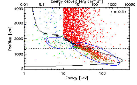
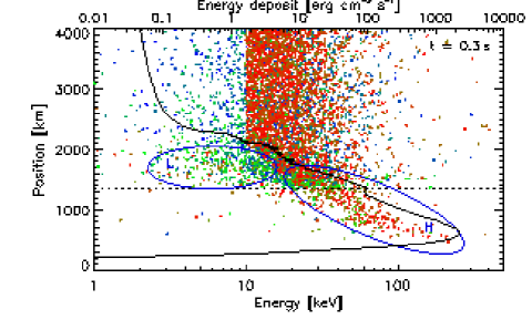
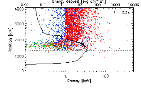
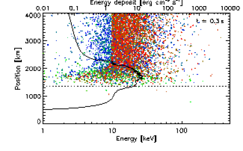
Figure 6: GRTTM distribution functions of non-thermal electron energies versus positions with a colour coded $M(\mu_{0})$ corresponding to the current density $j=6$ A m^-2 in the VAL C atmosphere at time $t=0.3$ s after the beam injection into the loop at its apex. Top: primary footpoint, bottom: secondary footpoint, left: $M^{\mathrm{FF}}$, right: $M^{\mathrm{SU}}$. The solid lines indicate the instantaneous energy deposits corresponding to $\mathcal{F}_{\mathrm{0}}/2=2.5\times 10^{9}$ erg cm^-2 s^-1, the dotted horizontal lines the bottom boundary of the magnetic mirror and the blue ellipses labelled L and H denote tails in the particle distribution function. Only the vicinity of the footpoints are displayed.

To distinguish the effects of the $\mu$-distribution and magnetic field convergence, Table 1 also lists the characteristics of CTTM for the case of no magnetic mirror, i.e. $R_{\mathrm{m}}=1$. It shows that it is the magnetic field convergence that significantly influences $\mathcal{F_{\mathrm{R}}}/\mathcal{F}_{\mathrm{0}}$ and $\mathcal{E}_{\mathrm{ch}}$ in the case of $M^{\mathrm{SU}}$.

A comparison of energy deposits for both considered initial $\mu$-distributions is shown in Fig. 5 (left). Because the adopted energy flux for both models considering secondary re-acceleration $\mathcal{F}_{\mathrm{0}}/2=2.5\times 10^{9}$ erg cm^-2 s^-1 is unrealistically low in the context of CTTM and flare physics, we also plot energy deposits for the much higher and more realistic value ${\mathcal{F}}_{\mathrm{0}}/2=5\times 10^{10}$ erg cm^-2 s^-1. The results corresponding to this flux will be used as a basis for comparison with the energy deposits and HXR spectra obtained from the models involving the secondary acceleration mechanisms. The chromospheric energy deposit $\mathcal{E}_{\mathrm{ch}}$ scales linearly with ${\mathcal{F}}_{\mathrm{0}}$ (see Table 1), and the positions of energy deposit maxima are almost identical for all the considered cases approximately corresponding to the placement of the lower boundary of the magnetic mirror $s_{\max}=1.36$ Mm. The peak in the energy deposits at $s_{\max}$ and their steep decrease above it (see Fig. 5, left) are caused by the constricted magnetic flux tube. The influence of the initial $\mu$-distribution is obvious. For the $M^{\mathrm{FF}}$ case, particles have a greater chance of passing through the magnetic mirror and thus of depositing their energy into the deeper layers. In the $M^{\mathrm{SU}}$ case, when the particles reach the thick-target region and the region of strongly converging field, their pitch angles are generally higher: compare the left-hand and right-hand panels of Fig. 4. Therefore the probability that an electron passes through the magnetic mirror is strongly reduced. This naturally explains the systematic enhancements in the energy deposits for $M^{\mathrm{SU}}$ in the layers above and the decrease in the layers below the lower boundary of the magnetic mirror in comparison with the $M^{\mathrm{FF}}$ case.

The corresponding HXR spectra are shown in Fig. 5 (right), and their parameters are summarised in Table 1. As expected, the HXR intensity $I_{25\,\mathrm{keV}}$ scales linearly with the chromospheric deposit $\mathcal{E}_{\mathrm{ch}}$ or the energy flux ${\mathcal{F}}_{\mathrm{0}}$. Majority of the total X-ray emission, i.e. summed over the whole loop, comes from the regions below the bottom boundary of the magnetic mirror. As explained above, the number of particles passing through the magnetic mirror is lower in the $M^{\mathrm{SU}}$ case than for $M^{\mathrm{FF}}$, therefore the HXR emission corresponding to $M^{\mathrm{FF}}$ is more intense than the emission of $M^{\mathrm{SU}}$.

HXR spectra are steeper in the $M^{\mathrm{SU}}$ case owing to presence of magnetic field convergence – compare $R_{\mathrm{m}}=1$ and 5 in Table 1. Fitted beam injected energy flux agrees well (within 20%) with the $\mathcal{E}_{\mathrm{ch}}$, whereas $\delta_{\mathrm{p}}^{\prime}$ and $E_{0}^{\prime}$ are the same as those of the injected power law. An exception is the larger $\delta_{\mathrm{p}}^{\prime}$ in the $M^{\mathrm{SU}}$ case, which corresponds to the mentioned HXR spectral behaviour and the fact that the spectral fitting does not take the scattering induced by change in $B$ into account.

3.2 GRTTM

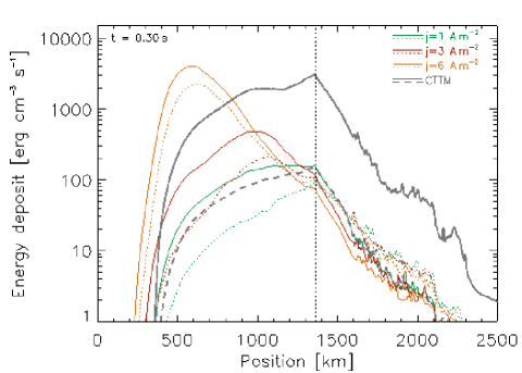
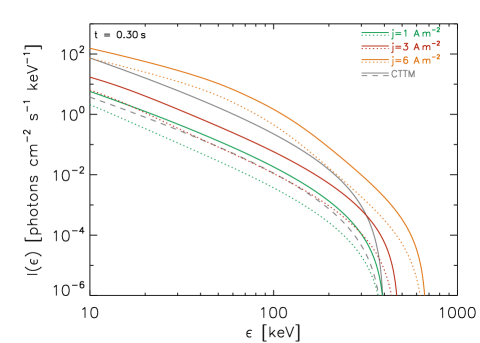
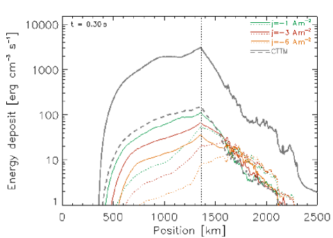
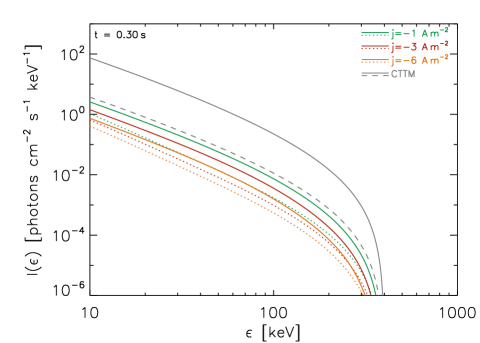
Figure 7: GRTTM instantaneous energy deposits (left) and HXR spectra (right) for the primary (top) and secondary (bottom) footpoints and the VAL C atmosphere at $t=0.3$ s. The green, red, and orange solid ($M^{\mathrm{FF}}$) and dotted ($M^{\mathrm{SU}}$) lines correspond to the current densities $j=1,3,6$ A m^-2, respectively, and to the energy flux $\mathcal{F}_{\mathrm{0}}/2=2.5\times 10^{9}$ erg cm^-2 s^-1. The grey dashed and solid lines correspond to the CTTM with $\mathcal{F}_{\mathrm{0}}/2=2.5\times 10^{9}$ and $5\times 10^{10}$ erg cm^-2 s^-1, respectively. The dotted straight vertical line indicates the bottom boundary of the magnetic mirror. The HXR spectra are integrated over one half of the loop.

The effects of static (global) electric field ${\bf E}_{\mathrm{G}}$ was studied for current densities in the range from 1 A m^-2 to 6 A m^-2. The distribution functions of non-thermal electrons for current density $j=6$ A m^-2 and time $t=0.3$ s after the beam injection into the loop at its apex are shown in Fig. 6. In the upper left-hand panel, two tails of particles can be identified in the primary footpoint and the $M^{\mathrm{FF}}$ case. A faint low-energy tail at energies $E<20$ keV, located above the bottom boundary of the magnetic mirror, is predominantly formed of particles with $\mu\leq 0$ (see the regions labelled L in Fig. 6). Its formation mechanism corresponds to the CTTM, i.e. to the particle deceleration related to the collisional energy losses in the target plasma and to the combined effects of particle scattering and magnetic field convergence, compare with Fig. 4 (left). This tail becomes more apparent for distributions that correspond to lower $j$ (see Fig. 4). On the other hand, a prominent high-energy tail, on energies from 20 to 300 keV stretching from 1.7 to 0.5 Mm (see the regions labelled H in Fig. 6), does not have any counterpart in Fig. 4 for the CTTM. The tail is formed of re-accelerated and relatively focussed particles with $\mu\approx 1$. Another obvious effects of ${\bf E}_{\mathrm{G}}$ are the increase in beam penetration depth with growing $j$ and a weakening of the population of reflected and back-scattered particles propagating towards the secondary footpoint that corresponds to 0.7% of the initial beam flux only, see Fig. 8 (left).

Figure 6 (top right, $M^{\mathrm{SU}}$ case) exhibits essentially the same features. The most apparent distinctions between the two distributions are a much richer population of particles in the low-energy tail located above the bottom boundary of the magnetic mirror and the existence of a relatively rich population of reflected and back-scattered particles with $\mu<0$ (on all energies) propagating towards the secondary footpoint reaching approximately 30% of the initial flux (see Fig. 8, bottom left). The differences between the distributions corresponding to $M^{\mathrm{FF}}$ and $M^{\mathrm{SU}}$ cases are solely effects of the initial $\mu$-distribution.

The situation at the secondary footpoint is shown in Fig. 6 (bottom). In addition to the effect of Coulomb collisions, the field ${\bf E}_{\mathrm{G}}$ constantly decreases the parallel velocity component of the particles propagating towards the secondary footpoint. This results in the formation of an enhanced low-energy tail in the particle distribution functions located above the bottom boundary of the magnetic mirror. Another obvious feature is a rich population of reflected or back-scattered particles corresponding approximately to 15% and 54% of the initial beam flux for the $M^{\mathrm{FF}}$ and $M^{\mathrm{SU}}$ cases, respectively (see Fig. 8, bottom left). These particles are accelerated by the global field ${\bf E}_{\mathrm{G}}$ back, towards the primary footpoint.

Table 2: Summary of results for the GRTTM with $\mathcal{F}_{0}/2=2.5\times 10^{9}$ erg cm^-2 s^-1.

Footpoint	${j}$	$\mathcal{F_{\mathrm{R}}}/\mathcal{F}_{\mathrm{0}}$	$\mathcal{E}_{\mathrm{ch}}/10^{9}$	$s_{\max}$	$I_{25\,\mathrm{keV}}$	$\gamma_{25\,\mathrm{keV}}$	$\mathcal{F}_{\mathrm{0}}^{\prime}/2\times 10^{9}$, $\delta^{\prime}_{\mathrm{p}}$, $E^{\prime}_{0}$
	[A m-2]	[%]	[erg s-1]	[Mm]	[cm-2 s-1 keV-1]		[erg cm-2 s-1], , [keV]
	1.0	3.1 (37)	2.8 (1.7)	1.2 (1.4)	0.71 (0.18)	2.4 (2.7)	3.3, 3.0, 12 (1.6, 3.4, 11)
	2.0	2.2 (36)	4.2 (2.1)	1.1 (1.1)	1.2 (0.29)	2.4 (2.7)	4.5, 3.0, 15 (2.2, 3.5, 13)
Primary	3.0	1.6 (33)	5.5 (3.0)	0.98 (1.1)	2.2 (0.56)	2.5 (2.9)	6.7, 3.1, 20 (3.2, 3.6, 17)
	4.0	1.5 (33)	7.7 (4.7)	0.87 (0.94)	5.0 (1.5)	2.40 (2.9)	10, 3.3, 30 (4.7, 3.7, 25)
	5.0	0.92 (32)	15 (7.7)	0.80 (0.83)	13 (4.5)	2.0 (2.3)	17, 3.5, 48 (7.7, 3.9, 39)
	6.0	0.69 (31)	30 (18)	0.60 (0.63)	38 (17)	1.7 (1.7)	35, 4.5, 100 (17, 4.8, 88)
	1.0	5.1 (42)	1.9 (1.2)	1.4 (1.4)	0.31 (0.086)	2.4 (2.7)	2.0, 3.0, 9 (1.0, 3.5, 10)
	2.0	6.6 (43)	1.5 (1.0)	1.4 (1.4)	0.22 (0.066)	2.4 (2.7)	1.6, 3.1, 9 (0.82, 3.5, 10)
Secondary	3.0	8.6 (47)	1.4 (0.89)	1.4 (1.6)	0.16 (0.053)	2.4 (2.7)	1.3, 3.1, 8 (0.70, 3.5, 10)
	4.0	11 (51)	1.2 (0.82)	1.4 (1.6)	0.13 (0.044)	2.4 (2.7)	1.0, 3.1, 8 (0.61, 3.6, 10)
	5.0	12 (55)	1.1 (0.71)	1.4 (1.7)	0.10 (0.034)	2.4 (2.8)	0.87, 3.1, 8 (0.52, 3.6, 10)
	6.0	15 (54)	0.93 (0.64)	1.4 (1.7)	0.081 (0.032)	2.5 (2.8)	0.74, 3.2, 8 (0.47, 3.6, 10)

     

   

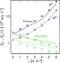
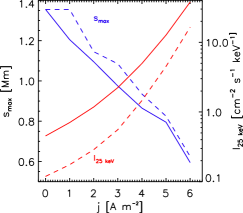
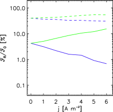
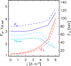
Figure 8: GRTTM summary of calculated parameters of chromospheric bombardment for various current densities $j$. The solid lines and asterisks denote the $M^{\mathrm{FF}}$, the dashed lines and triangles denote the $M^{\mathrm{SU}}$. Left: chromospheric energy deposit $\mathcal{E}_{\mathrm{ch}}$ (lines) and fitted energy flux $\mathcal{F}_{\mathrm{0}}^{\prime}$ (symbols) (top), the ratio $\mathcal{F}_{\mathrm{R}}/\mathcal{F}_{\mathrm{0}}$ (bottom) for the primary (blue) and secondary (green) footpoints. Right: position of energy deposit maximum $s_{\max}$ and HXR intensity $I_{25\,\mathrm{keV}}$ (top), HXR spectral index $\gamma_{25\,\mathrm{keV}}$, fitted electron beam spectral index $\delta^{\prime}_{\mathrm{p}}$ and low-energy cutoff $E^{\prime}_{0}$ (bottom) only for the primary footpoint.

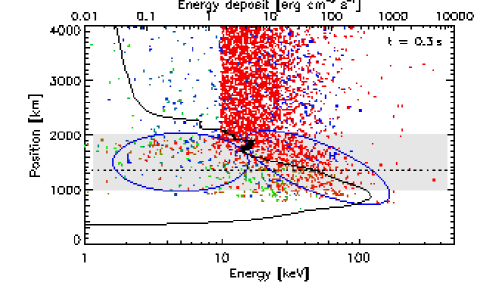
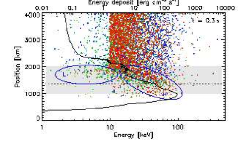
Figure 9: LRTTM ${{\bf E}_{\mathrm{L}}}$-I type distribution functions of the non-thermal electron energies versus positions with a colour-coded $M(\mu_{0})$ corresponding to $\overline{E_{\mathrm{L}}}=0$ V m^-1 and $\mbox{var}(E_{\mathrm{L}})=1$ V m^-1 in the VAL C atmosphere at time $t=0.3$ s after the beam injection into the loop at its apex. Left: $M^{\mathrm{FF}}$; right: $M^{\mathrm{SU}}$. The solid lines indicate the instantaneous energy deposits corresponding to $\mathcal{F}_{\mathrm{0}}/2=2.5\times 10^{9}$ erg cm^-2 s^-1, the dotted horizontal lines the bottom boundary of the magnetic mirror, the grey area the secondary re-acceleration region, and the blue ellipses labelled L and H denote tails in the particle distribution function. Only the vicinity of the footpoints is displayed.

The instantaneous energy deposits and HXR spectra for both the primary and secondary footpoints and various current densities are shown in Fig. 7, and the quantitative results, some of them only for the primary footpoint, are summarised in Fig. 8 (see Table 2 for complete results). The magnitudes and spatial distributions of energy deposits in the atmosphere, as well as the production of HXR photons, are extremely sensitive to the current densities in the threads. According to our simulations, the current density $j=6$ A m^-2 increases $\mathcal{E}_{\mathrm{ch}}$ at the primary footpoint of one order and $I_{25\,\mathrm{keV}}$ of approximately two orders (see Fig. 8). Moreover, this HXR spectrum is more intense than the spectrum of pure CTTM with $\mathcal{F}_{0}/2=5\times 10^{10}$ erg cm^-2 s^-1 (see Fig. 7, top right). The presence of $j$ also considerably changes the distribution of the energy deposit in the thick-target region. The maximum of the energy deposit $s_{\max}$ is substantially shifted towards the photosphere (compare the results for $j=0$ corresponding to the CTTM and for $j>0$ in the top right of Fig. 8), and the energy is deposited in a much narrower region in the chromosphere (see the top left of Fig. 7). In the case of $j=6$ A m^-2, $\mathcal{E}_{\mathrm{ch}}$ is comparable to $\mathcal{F}_{0}/2=5\times 10^{10}$ erg cm^-2 s^-1 of pure CTTM, however the spatial distribution is completely different.

HXR emission of the primary footpoint comes predominantly from regions well below the bottom of the magnetic mirror, close to temperature minimum for $j\gtrsim 3$ A m^-2 and photon energies $\gtrsim 50$ keV. As $j$ increases, HXR spectra get more intense and flatter at deka-keV energies, and the maximum photon energy is shifted to higher energies. This is all consistent with the presence of the high-energy electrons accelerated by ${\bf E}_{\mathrm{G}}$ below the magnetic mirror. Although the HXR power-law index $\gamma_{25\,\mathrm{keV}}$ tends to harden as $j$ increases, the fitted CTTM injected electron power-law index $\delta_{\mathrm{p}}^{\prime}$ becomes steeper. However, at the same time, the low-energy cutoff $E_{0}^{\prime}$ rises to deka-keV values, causing decrease in $\gamma_{25\,\mathrm{keV}}$ – see fitted parameters in Fig. 8 (bottom right).

The model of $j=1$ A m^-2 is similar to the CTTM situation; i.e. similar formation heights of HXR, spectral shape of photon spectrum (Fig. 7, left), and fitted electron distribution (Fig. 8, bottom right). In the case of $j=6$ A m^-2, the HXR spectra are extremely flat below $\sim$40 keV with $E_{0}^{\prime}\sim 100$ keV. Such low-energy cutoffs are not found from observations, therefore this case could represent a limit of possible $j$ in flare loops.

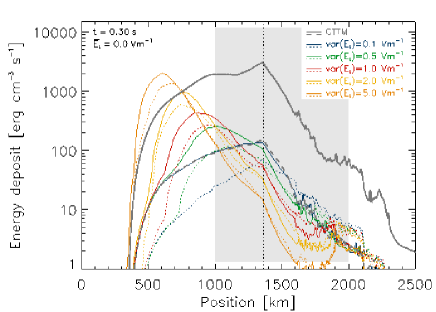
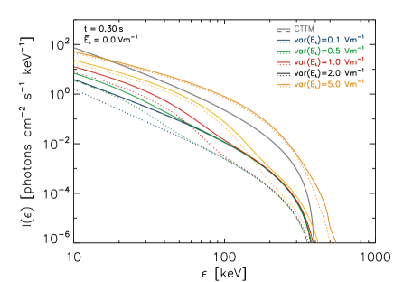
Figure 10: LRTTM ${{\bf E}_{\mathrm{L}}}$-I type instantaneous energy deposits (left) and HXR spectra (right) for the VAL C atmosphere at $t=0.3$ s. The solid ($M^{\mathrm{FF}}$) and dotted ($M^{\mathrm{SU}}$) blue, green, red, yellow, and orange lines correspond to $\overline{E_{\mathrm{L}}}=0$ V m^-1 and $\mbox{var}(E_{\mathrm{L}})=0.1,0.5,1,2,5$ V m^-1, respectively, and energy flux $\mathcal{F}_{\mathrm{0}}/2=2.5\times 10^{9}$ erg cm^-2 s^-1. The dashed and solid grey lines correspond to the CTTM with $\mathcal{F}_{\mathrm{0}}/2=2.5\times 10^{9}$ and $5\times 10^{10}$ erg cm^-2 s^-1, respectively. The dotted straight vertical line indicates the bottom boundary of the magnetic mirror, the grey area the secondary re-acceleration region. The HXR spectra are integrated over one half of the loop.

The situation at the secondary footpoint is different (see Fig. 7, bottom). Because a part of energy carried by non-thermal particles is drained due to the actuation of ${\bf E}_{\mathrm{G}}$, the resulting chromospheric energy deposits for a particular $j$ are smaller than at the primary footpoint. As expected, this behaviour steeply increases with $j$. Although the HXR spectra of the secondary footpoint are less intense than the spectrum of pure CTTM, the overall spectral shape is not changed significantly. Consequently, the fitted injected electron beam parameters show only a decrease of $\mathcal{F}_{\mathrm{0}}^{\prime}$ consistent with lower $\mathcal{E}_{\mathrm{ch}}$ (see Fig. 8, top left) and Table 2.

Table 3: Summary of results for the LRTTM with $\mathcal{F}_{0}/2=2.5\times 10^{9}$ erg cm^-2 s^-1.

$\overline{E_{\mathrm{L}}}$	$\mbox{var}({E_{\mathrm{L}}})$	$\mathcal{F_{\mathrm{R}}}/\mathcal{F}_{\mathrm{0}}$	$\mathcal{E}_{\mathrm{ch}}/10^{9}$	$s_{\max}$	$I_{25\,\mathrm{keV}}$	$\gamma_{25\,\mathrm{keV}}$	$\mathcal{F}_{\mathrm{0}}^{\prime}/2\times 10^{9}$, $\delta^{\prime}_{\mathrm{p}}$, $E^{\prime}_{0}$
[V m-1]	[V m-1]	[%]	[erg s-1]	[Mm]	[cm-2 s-1 keV-1]		[erg cm-2 s-1, , keV]
0.0	0.1	5.8 (41)	2.2 (1.4)	1.3 (1.4)	0.46 (0.12)	2.4 (2.7)	2.2, 3.0, 12 (1.2, 3.5, 11)
	0.5	21 (78)	3.0 (1.7)	1.0 (1.1)	0.79 (0.32)	2.8 (3.3)	2.9, 3.7, 24 (1.5, 4.4, 25)
	1.0	31 (120)	3.9 (2.5)	0.87 (0.96)	2.0 (1.2)	2.4 (2.5)	4.1, 4.4, 41 (2.6, 4.9, 42)
	2.0	44 (130)	6.4 (4.5)	0.78 (0.76)	4.8 (3.6)	1.9 (1.9)	6.2, 4.8, 70 (4.7, 5.0, 71)
	3.0	68 (140)	7.0 (5.5)	0.69 (0.71)	7.5 (6.0)	1.8 (1.8)	7.9, 4.6, 93 (6.4, 4.8, 93)
	4.0	77 (170)	9.1 (7.5)	0.66 (0.70)	10 (8.3)	1.7 (1.7)	9.7, 4.5, 110 (7.9, 4.6, 110)
	5.0	90 (160)	12 (8.6)	0.61 (0.68)	13 (11)	1.6 (1.6)	11, 4.3, 130 (9.8, 4.4, 130)
0.1	0.0	0.05 (23)	7.5 (6.5)	0.91 (0.94)	4.2 (2.8)	2.4 (2.6)	8.7, 6.0, 47 (6.5, 9.0, 48)
	0.5	0.63 (37)	8.3 (6.1)	0.88 (0.89)	4.7 (3.3)	2.3 (2.40)	8.7, 5.7, 51 (6.6, 7.0, 52)
	1.0	3.2 (55)	8.7 (8.2)	0.82 (0.84)	6.2 (4.6)	2.1 (2.1)	9.5, 5.6, 61 (7.3, 6.0, 61)
	2.0	17 (78)	10 (8.7)	0.72 (0.74)	8.7 (7.3)	1.9 (1.9)	10, 5.8, 84 (8.6, 5.8, 85)
	3.0	37 (100)	12 (8.7)	0.68 (0.70)	11 (9.8)	1.7 (1.7)	11, 4.8, 100 (9.9, 5.0, 110)
	4.0	65 (120)	9.0 (12)	0.63 (0.63)	13 (12)	1.6 (1.6)	12, 4.6, 120 (11, 4.7, 130)
	5.0	76 (150)	13 (11)	0.63 (0.65)	16 (14)	1.6 (1.6)	13, 4.4, 140 (12, 4.4, 140)

3.3 LRTTM

3.3.1 ${{\bf E}_{\mathrm{L}}}$-I type

The non-thermal electron distribution functions for the stochastic field with $\overline{E_{\mathrm{L}}}=0$ V m^-1 and $\mbox{var}({E}_{\mathrm{L}})=1$ V m^-1 in the VAL C atmosphere and time $t=0.3$ s after the beam injection into the loop at its apex are shown in Fig. 9. In both panels two kinds of particle populations can be identified: a conspicuous high-energy tail fuzzy in energies at particular height sections (see the regions labelled H), and an inconspicuous low-energy tail (see the regions labelled L).

The high-energy tail is located within the re-acceleration region on energies from 10 to 100 keV. It indicates that the net re-acceleration of particles occurs even though any electron in the re-acceleration region has an equal probability of encountering stochastic field ${{\bf E}_{\mathrm{L}}}$ (normally distributed) of parallel or anti-parallel orientation relative to $\mu=1$. The net acceleration in this type of electric field is a consequence of inverse proportionality between the electron collisional energy loss and energy $\mbox{d}E/\mbox{d}z\propto 1/E$, $z$ being the column density (Emslie, 1978). The energy gain of re-accelerated electrons increases with $\mbox{var}({E}_{\mathrm{L}})$ similar to the fuzziness of the high-energy tails and the fluxes of backwards moving electrons (with $\mu<0$). The ratio $\mathcal{F_{\mathrm{R}}}/\mathcal{F}_{\mathrm{0}}$ corresponding to $\mbox{var}({{E}_{\mathrm{L}}})=1$ V m^-1 is approximately 31% and 120% for the $M^{\mathrm{FF}}$ and $M^{\mathrm{SU}}$ cases, respectively; i.e., in the latter case the backward energy flux exceeds the initial flux propagating downwards from the corona (see Fig. 11, right). Another effect of growing $\mbox{var}{({E}_{\mathrm{L}})}$ is a decrease in the electron population having $\mu$ distinct from 1 or $-1$. Ultimately, for high values of $\mbox{var}{({E}_{\mathrm{L}})}$, only particles with $\mu$ either close to 1 or $-1$ are present in the distribution, so the $\mu$-distribution then copies the directional distribution of the re-accelerating field.

The inconspicuous low-energy tail spreads from the top of the re-acceleration region to the lower boundary of the magnetic mirror, and it is formed of particles of all possible pitch angles with energies under 20 keV. It is shifted higher into the chromosphere in comparison to the low-energy tail in the CTTM case (see Fig. 4). As $\mbox{var}{({E}_{\mathrm{L}})}$ increases, the low-energy tail becomes less distinct and its location is shifted higher towards the upper boundary of the re-acceleration region. The low-energy tail is formed by concerted actuation of Coulomb collisions and alternating stochastic field.

The energy deposits and HXR spectra corresponding to various values of $\mbox{var}(E_{\mathrm{L}})$ in the range from 0.1 to 5 V m^-1 are shown in Fig. 10 and their main parameters $\mathcal{E}_{\mathrm{ch}}$, $s_{\max}$, $I_{25\,\mathrm{keV}}$, and $\gamma_{25\,\mathrm{keV}}$ are displayed in left-hand panels of Figs. 11 and 12 and summarised in Table 3.

The behaviour of the energy deposits is similar to the GRTTM of the primary footpoint. They increase with $\mbox{var}{({E}_{\mathrm{L}})}$, $s_{\max}$ are shifted to the deeper layers, and the energy is deposited into an even narrower chromospheric region. For the lowest studied value $\mbox{var}(E_{\mathrm{L}})=0.1$ V m^-1, we obtained practically no change in all followed parameters relative to the CTTM with an identical initial flux (see Figs. 10, 11 and 12).

On the other hand, for the maximum value $\mbox{var}(E_{\mathrm{L}})=5$ V m^-1 there is half an order increase in $\mathcal{E}_{\mathrm{ch}}$ and a substantial shift of $s_{\max}$ towards the photosphere ($\sim$750 km) for both initial $\mu$-distributions. The value of $I_{25\,\mathrm{keV}}$ increases considerably ($28\times$ for the $M^{\mathrm{FF}}$ and $10^{2}\times$ for the $M^{\mathrm{SU}}$ case) relative to the CTTM with an identical initial flux (see Fig. 12, left).

Again, hard X-ray emission comes from the regions below the magnetic mirror. As for GRTTM case, as $\mbox{var}(E_{\mathrm{L}})$ increases, the LRTTM hard X-ray spectra at $\sim$25 keV become flatter (see $\gamma_{25\,\mathrm{keV}}$ in Fig. 12, left). Values of $\mbox{var}(E_{\mathrm{L}})\geq 2$ V m^-1 result in extremely flat photon spectra. On the other hand, the LRTTM X-ray spectra exhibit a double break or a local sudden decrease; see e.g. the spectrum in the $\sim$50 – 100 keV range corresponding to $\mbox{var}(E_{\mathrm{L}})=1.0$ V m^-1 in Fig. 10, right. Such spectral shapes affect the fitted CTTM electron distributions and result in high values of $E^{\prime}_{0}$ (located approximately at the energy of a double break) and higher values of $\delta^{\prime}_{0}$ (see Fig. 12, bottom left). As $\mbox{var}(E_{\mathrm{L}})$ rises, $E^{\prime}_{0}$ still increases but $\delta_{0}^{\prime}$ stays almost constant, i.e. 4 – 5. The model of $\mbox{var}(E_{\mathrm{L}})=5$ V m^-1 presents a limit, and the hard X-ray spectrum is consistent with a rather flat electron flux spectrum of high $E^{\prime}_{0}$. Although the spectrum is more intense than the spectrum of pure CTTM with $\mathcal{F}_{\mathrm{0}}/2=5\times 10^{10}$ erg cm^-2 s^-1 (i.e. 20$\times$ higher than the initial flux used in this model), owing to the high value of $E^{\prime}_{0}$, the fitted electron flux is lower and consistent with the energy deposit in the chromosphere $\mathcal{E}_{\mathrm{ch}}$ (see Fig. 11, left).

3.3.2 ${{\bf E}_{\mathrm{L}}}$-II type

The effects of local re-acceleration due to the stochastic field ${{\bf E}_{\mathrm{L}}}$ with $\overline{E_{\mathrm{L}}}\neq 0$ are demonstrated for the case with $\overline{E_{\mathrm{L}}}=0.1$ V m^-1 and $\mbox{var}(E_{\mathrm{L}})=0.5$ V m^-1 (see the distribution functions for $M^{\mathrm{FF}}$ and $M^{\mathrm{SU}}$ cases in Fig. 13). The re-acceleration process again results in formation of fuzzy high-energy tail of particles situated in the secondary acceleration region and covering the energy range from 10 to 100 keV approximately (see the regions labelled H). The mean energy reached by the re-accelerated electrons at the lower boundary of the re-acceleration region steeply increases with $\overline{E_{\mathrm{L}}}$, and at the same time the maximum of energy deposit shifts towards the deeper layers. The mean value of ${{\bf E}_{\mathrm{L}}}$ also has a strong focussing effect on the re-accelerated electrons. The latter effect reduces the ratio of backscattered and reflected particle flux to the initial flux $\mathcal{F_{\mathrm{R}}}/\mathcal{F}_{\mathrm{0}}$ to less than 1% for the $M^{\mathrm{FF}}$ and to 37% for the $M^{\mathrm{SU}}$ case, respectively: compare values of $\mathcal{F_{\mathrm{R}}}/\mathcal{F}_{\mathrm{0}}$ for the individual field types and parameters of ${{\bf E}_{\mathrm{L}}}$ displayed in Fig. 11 (right). The value of $\mbox{var}(E_{\mathrm{L}})$ plays a similar role to what is described above for the ${{\bf E}_{\mathrm{L}}}$-I type. In comparison with the effects of $\overline{E_{\mathrm{L}}}$, it only weakly influences the energy gain of electrons at the lower boundary of the re-acceleration region, it increases the fuzziness of the high-energy tail and the flux of backwards moving electrons (with $\mu<0$). For high values of $\mbox{var}(E_{\mathrm{L}})$ we also see a decrease in electrons having $\mu$ other than close to 1 and $-1$, which is again the effect of imprint of the directional distribution of ${{\bf E}_{\mathrm{L}}}$ on the electron $\mu$-distribution, which was also found for the stochastic field type ${{\bf E}_{\mathrm{L}}}$-I.

 

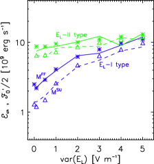
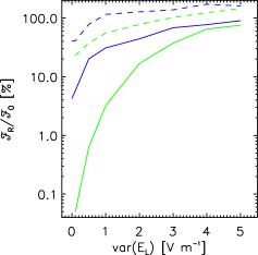
Figure 11: LRTTM ${\bf E}_{\mathrm{L}}$-I (blue) and ${\bf E}_{\mathrm{L}}$-II (green) (for $\overline{E_{\mathrm{L}}}=0.1$ V m^-1) chromospheric energy deposits $\mathcal{E}_{\mathrm{ch}}$ (lines) and fitted energy flux $\mathcal{F}_{\mathrm{0}}^{\prime}$ (symbols) (left) and the ratio $\mathcal{F}_{\mathrm{R}}/\mathcal{F}_{\mathrm{0}}$ (right) for various $\mbox{var}(E_{\mathrm{L}})$. Solid lines and asterisks denote $M^{\mathrm{FF}}$; dashed lines and triangles denote $M^{\mathrm{SU}}$.

 

 

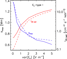
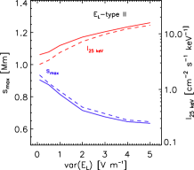
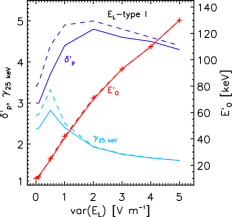
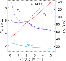
Figure 12: LRTTM ${\bf E}_{\mathrm{L}}$-I (left) and ${\bf E}_{\mathrm{L}}$-II (right) (for $\overline{E_{\mathrm{L}}}=0.1$ V m^-1) summary of calculated and fitted parameters of chromospheric bombardment for various values of $\mbox{var}({E_{\mathrm{L}}})$. Top: position of energy deposit maximum $s_{\max}$ and HXR intensity $I_{25\,\mathrm{keV}}$. Bottom: HXR spectral index $\gamma_{25\,\mathrm{keV}}$ and fitted electron beam spectral index $\delta^{\prime}_{\mathrm{p}}$ and low-energy cutoff $E^{\prime}_{0}$. The solid and dashed lines denote $M^{\mathrm{FF}}$ and $M^{\mathrm{SU}}$, respectively.

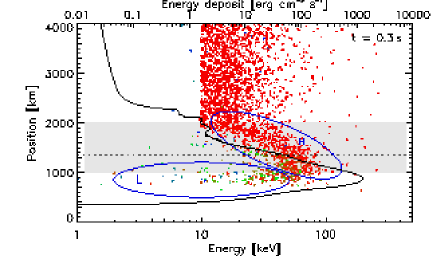
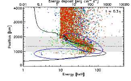
Figure 13: LRTTM ${{\bf E}_{\mathrm{L}}}$-II type distribution functions of the non-thermal electron energies versus positions with a colour coded $M(\mu)$ corresponding to $\overline{E_{\mathrm{L}}}=0.1$ V m^-1 and $\mbox{var}(E_{\mathrm{L}})=0.5$ V m^-1 in the VAL C atmosphere at time $t=0.3$ s after the beam injection into the loop at its apex. Left: $M^{\mathrm{FF}}$, right: $M^{\mathrm{SU}}$. The solid lines indicate the instantaneous energy deposits corresponding to $\mathcal{F}_{\mathrm{0}}/2=2.5\times 10^{9}$ erg cm^-2 s^-1, the dotted horizontal lines the bottom boundary of the magnetic mirror, the grey area the secondary re-acceleration region, and the blue ellipses labelled L and H denote tails in the particle distribution function. Only the vicinity of the footpoints is displayed.

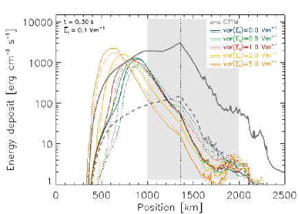
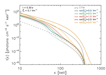
Figure 14: LRTTM ${{\bf E}_{\mathrm{L}}}$-II type instantaneous energy deposits (left) and HXR spectra (right) for the VAL C atmosphere at $t=0.3$ s. The solid ($M^{\mathrm{FF}}$) and dotted ($M^{\mathrm{SU}}$) blue, green, red, yellow, and orange lines correspond to $\overline{E_{\mathrm{L}}}=0.1$ V m^-1 and $\mbox{var}(E_{\mathrm{L}})=0.1,0.5,1,2,5\leavevmode\nobreak\$ V m^-1, respectively and energy flux $\mathcal{F}_{\mathrm{0}}/2=2.5\times 10^{9}$ erg cm^-2 s^-1. The dashed and solid grey lines correspond to the CTTM with $\mathcal{F}_{\mathrm{0}}/2=2.5\times 10^{9}$ and $5\times 10^{10}$ erg cm^-2 s^-1, respectively. The dotted straight vertical line indicates the bottom boundary of the magnetic mirror, the grey area the secondary re-acceleration region. The HXR spectra are integrated over one half of the loop.

The stochastic field of $\overline{E_{\mathrm{L}}}=0.1$ V m^-1 and $\mbox{var}(E_{\mathrm{L}})=0.5$ V m^-1 (see Fig. 13) practically ceases the formation of the low-energy tail of particles located in the region between the upper boundary of the re-acceleration region and the lower boundary of the magnetic mirror found in the distribution functions corresponding to the CTTM, GRTTM, and LRTTM ${{\bf E}_{\mathrm{L}}}$-I type (see Figs. 4, 6, and 9). It forms either for lower values of $\overline{E_{\mathrm{L}}}$, which is too small to compensate for the collisional energy losses of the electrons in the region above the lower boundary of the magnetic mirror, or for greater values of $\mbox{var}(E_{\mathrm{L}})$, when the interactions of beam electrons with the stochastic component of ${{\bf E}_{\mathrm{L}}}$ lead to its formation. On the other hand, a new tail of particles is formed on energies from approximately 1 to 100 keV in the region under the lower boundary of the re-acceleration region where the re-accelerated particles are quickly thermalised (see the regions labelled L).

The energy deposits and HXR spectra for $\overline{E_{\mathrm{L}}}=0.1$ V m^-1 and various values of $\mbox{var}(E_{\mathrm{L}})$ from 0 to 5 V m^-1 are plotted in Fig. 14, and the parameters $\mathcal{E}_{\mathrm{ch}}$, $s_{\max}$, $I_{25\,\mathrm{keV}}$, and $\gamma_{25\,\mathrm{keV}}$ are displayed in the left-hand and right-hand panels of Figs. 11 and 12, respectively, and summarised in Table 3. The general behaviour of $\mathcal{E}_{\mathrm{ch}}$ and $s_{\max}$ is similar to the GRTTM of primary footpoint and LRTTM ${{\bf E}_{\mathrm{L}}}$-I type. They are very sensitive to the static component $\overline{E_{\mathrm{L}}}$ of the stochastic field and only moderately sensitive to the stochastic component $\mbox{var}(E_{\mathrm{L}})$. Even for $\mbox{var}(E_{\mathrm{L}})=0$ and $\overline{E_{\mathrm{L}}}=0.1$ V m^-1, there is an appreciable increase of $\mathcal{E}_{\mathrm{ch}}$ ($3.6\times$ for the $M^{\mathrm{FF}}$ and $5.5\times$ for the $M^{\mathrm{SU}}$ case) and a shift of $s_{\max}$ of approximately 450 km towards the photosphere and substantial growth in HXR production ($I_{25\,\mathrm{keV}}$ increases of by an order of magnitude for both initial $\mu$-distributions relative to the CTTM with an identical initial flux). For the identical value of $\overline{E_{\mathrm{L}}}$ and the maximum value of $\mbox{var}(E_{\mathrm{L}})=5$ V m^-1, the increase in $\mathcal{E}_{\mathrm{ch}}$ is $5.5\times$ for the $M^{\mathrm{FF}}$ and $10\times$ for the $M^{\mathrm{SU}}$ case, the shift of $s_{\max}$ towards the photosphere of approximately 750 km (for both initial $\mu$-distributions), and a substantial increase in $I_{25\,\mathrm{keV}}$ ($35\times$ for the $M^{\mathrm{FF}}$ and almost $130\times$ for the $M^{\mathrm{SU}}$ case) relative to the CTTM with an identical initial flux. The power-law index $\gamma_{25\,\mathrm{keV}}$ tends to harden with increasing $\mbox{var}(E_{\mathrm{L}})$.

HXR spectra corresponding to the ${\bf E}_{\mathrm{L}}$-II type are distinct from the previous ones. Here, two re-accelerating processes are involved. The static component causes a significant increase of spectra at deka-keV energies, up to $\sim$40 keV, and a steep double break at energies above. Therefore, the corresponding fitted electron flux spectrum assuming pure CTTM shows quite a steep $\delta_{0}^{\prime}$ (see Fig. 12, bottom right). Such a steep double break is a consequence of a re-acceleration by a constant electric field. The energy at which it appears is related to the length of the re-acceleration region, i.e. the current sheet size. The larger the size, the steeper the double break and the higher energies at which it is located. The presence of the stochastic component introduces another shift of the double break to higher energies, likewise for the type I; as $\mbox{var}(E_{\mathrm{L}})$ increases, the double break is less prominent. Consequently, $E_{0}^{\prime}$ increases and $\delta_{0}^{\prime}$ decreases (see Figs. 12 and 14). When the stochastic component prevails, i.e. $\mbox{var}(E_{\mathrm{L}})\geq 2$ V m^-1, the hard X-ray spectra are of similar spectral shape to the ${\bf E}_{\mathrm{L}}$-I model but more intense.

4 Conclusions

We studied modifications of the CTTM by considering two types of secondary particle acceleration: GRTTM and LRTTM. In both cases the re-acceleration takes place during the transport of non-thermal particles, which are primarily accelerated in the corona. According to Brown et al. (2009), such a re-acceleration generally reduces collisional energy loss and Coulomb scattering and increases the life-time and penetration depth of particles.

In the case of GRTTM, the spatially varying direct electric field spreading along the whole magnetic strand from first to second footpoint re-accelerates the beam electrons towards the primary footpoint and decelerates them towards the secondary footpoint, thus producing an asymmetric heating of footpoints. The low electric plasma conductivity and increased current density due to magnetic field convergence are the key constraints for the functionality of this mechanism. The model was studied for the mirror ratio $R_{\mathrm{m}}=5$ and current densities $j\leq 6$ A m^-2. Significant re-acceleration is present for $j\gtrsim 3$ A m^-2, and for lower $j$ the model is similar to CTTM. However, a question arises as to whether such current densities are realistic. Although the current densities derived from magnetic field observations are two orders of magnitude lower (Guo et al., 2013), in the magnetic rope, especially in their unstable phase at the beginning of the flare, the current density in some filaments could reach these values: see the processes studied in Gordovskyy & Browning (2011, 2012); Gordovskyy et al. (2013). On the other hand, a current filamentation also means a decrease in the area where this re-acceleration can operate effectively. Finally, the GRTTM model inherently introduces an asymmetry on opposite sites of the magnetic rope. More observations are needed to check that some asymmetrical X-ray sources are caused by this effect.

Two types of electric field were considered for LRTTM: a purely stochastic field $\mbox{var}(E_{\mathrm{L}})\leq 5$  V m^-1 (${\bf E}_{\mathrm{L}}$-I type) and a combination of $\mbox{var}(E_{\mathrm{L}})$ and a static component $\overline{E_{\mathrm{L}}}=0.1$ V m^-1 (${\bf E}_{\mathrm{L}}$-II type). It has been shown that both types of electric fields produce a substantial secondary re-acceleration (${\bf E}_{\mathrm{L}}$-I type for $\mbox{var}(E_{\mathrm{L}})\gtrsim 0.5$ V m^-1, ${\bf E}_{\mathrm{L}}$-II type for all considered field parameters due to the static field component) with dominant energy propagating towards the photosphere.

Generally in all presented models, HXR spectra gets flatter below $\sim$30 keV and more intense on all energies as re-accelerating fields increase. The flattening then corresponds to an increase in the low-energy cutoff $E_{0}^{\prime}$ of the fitted electron distribution. The effect of flattening of HXR spectra below the low-energy cutoff can be seen in Brown et al. (2008, Fig. 1e). Extremely flat HXR spectra (related to $E_{0}^{\prime}\gtrsim 50$ keV) were obtained for GRTTM of $j=6$ A m^-2 and LRTTM $\mbox{var}(E_{\mathrm{L}})\geq 2$ V m^-1 (${\bf E}_{\mathrm{L}}$-I type). Such flat spectra or high values of $E_{0}^{\prime}$ are not reported from the observation, therefore those $j$ and $\mbox{var}(E_{\mathrm{L}})$ could represent limiting values. In addition, prominent double breaks at keV energies, present in the ${\bf E}_{\mathrm{L}}$-II cases, are not observed in HXR spectra. This suggests that our model of a constant re-accelerating field over a larger spatial scale, $\sim$1 Mm, is probably too simplistic.

For upper limit of model parameters, both models give similar results in several aspects (although the values are probably extreme, at least from the HXR signatures). At energies above 20 keV, the corresponding HXR spectra are more intense than the spectrum of pure CTTM with $20\times$ higher initial energy flux. GRTTM gives a comparable total chromospheric energy deposit. For the LRTTM the total energy deposits reach only about 30% of the latter value. The re-acceleration also leads to spatial redistribution of the chromospheric energy deposit with the bulk energy being deposited much deeper into the chromosphere and into a narrower layer in comparison to the CTTM. The heights of the energy-deposit maxima are thus substantially shifted towards the photosphere (of $\approx$800 km for both models). It is a consequence of the re-accelerating fields pushing the non-thermal electrons under the magnetic mirror and under the beam-stopping depth corresponding to the CTTM. The height above the photosphere decreases with both the current density for the GRTTM and with the mean value and variance of the stochastic field for the LRTTM. For the upper values of model parameters, we obtained the heights of energy-deposit maxima as only approximately 600 km. This is not far from the upper limits on heights of the flare white-light sources ($305\pm 170$ km and $195\pm 70$ km) found from observations (Martínez Oliveros et al., 2012).

To demonstrate how the secondary accelerating processes may lead to artificially high CTTM input energy fluxes, we followed a standard forward-fitting procedure for determining the injected electron spectrum from an observed X-ray spectrum. Although the spectral fitting does not take any re-acceleration into account, the fitted $\mathcal{F}_{0}^{\prime}$ agrees well (within $30\%$) with $\mathcal{E}_{\mathrm{ch}}$ in all simulations. This value can differ substantially from the injected total energy flux, therefore the fitted total energy flux (under assumption of pure CTTM) is related more to the energy deposit of re-accelerated particles than to the injected energy flux.

In general, both the considered models with secondary re-acceleration, GRTTM and LRTTM, allow loosening the requirements on the efficiency of coronal accelerator, thus decreasing the total number of particles involved in the impulsive phase of flares and the magnitude of the electron flux transported from the corona towards the photosphere, as needed to explain the observed HXR footpoint intensities. These findings agree with the results obtained by Brown et al. (2009) and Turkmani et al. (2006, 2005).