Low-Rank Modeling and Its Applications in Image Analysis

Abstract

Low-rank modeling generally refers to a class of methods that solve problems by representing variables of interest as low-rank matrices. It has achieved great success in various fields including computer vision, data mining, signal processing and bioinformatics. Recently, much progress has been made in theories, algorithms and applications of low-rank modeling, such as exact low-rank matrix recovery via convex programming and matrix completion applied to collaborative filtering. These advances have brought more and more attentions to this topic. In this paper, we review the recent advance of low-rank modeling, the state-of-the-art algorithms, and related applications in image analysis. We first give an overview to the concept of low-rank modeling and challenging problems in this area. Then, we summarize the models and algorithms for low-rank matrix recovery and illustrate their advantages and limitations with numerical experiments. Next, we introduce a few applications of low-rank modeling in the context of image analysis. Finally, we conclude this paper with some discussions.

1 Introduction

In many research fields the data to be analyzed often have high dimensionality, which brings great challenges to data analysis. Some examples include images in computer vision, documents in natural language processing, customers’ records in recommender systems, and genomics data in bioinformatics.

Fortunately, the high-dimensional data often lie in a low-dimensional subspace. Mathematically, if we represent each data point by a vector ${\mathbf{d}}_{i}\in\mathbb{R}^{m}$ and denote the entire dataset by a big matrix ${\mathbf{D}}=\left[{\mathbf{d}}_{1},\cdots,{\mathbf{d}}_{n}\right]$, the low-dimensionality assumption can be translated into the following low-rank assumption: $\mbox{rank}({\mathbf{D}})\ll\min(m,n)$. A typical example in computer vision is Lambertian reflectance, where ${\mathbf{d}}_{1},\cdots,{\mathbf{d}}_{n}$ correspond to a set of images of a convex Lambertian surface under various lighting conditions (Basri and Jacobs, 2003). Another example is from signal processing, where ${\mathbf{d}}_{i}$ represents a vector of signal intensities received by an antenna array at time point $i$. Interested readers are referred to (Markovsky, 2012, Chapter 1.3) for more low-rank examples.

In the real world, the raw data can hardly be perfectly low-rank due to the existence of noise. Therefore, the following model is more faithful to real situations

$${\mathbf{D}}={\mathbf{X}}+{\mathbf{E}},$$ (1)

where ${\mathbf{X}}$ corresponds to a low-rank component and ${\mathbf{E}}$ corresponds to the noise or error in measurements. Recovering the low-rank structure from noisy data becomes the centric task in many problems.

A conventional approach to finding the low-rank approximation is to solve the following optimization problem:

$$\min_{{\mathbf{X}}}~{} \|{\mathbf{D}}-{\mathbf{X}}\|_{F}^{2},$$

s.t. $$\mbox{rank}({\mathbf{X}})\leq r,$$ (2)

where $\|{\mathbf{Y}}\|_{F}=\sqrt{\sum_{ij}{Y_{ij}^{2}}}$ denotes the Frobenious norm of a matrix. Solving such a minimization problem can be interpreted as seeking the optimal rank-$r$ estimate of ${\mathbf{D}}$ in a least-squares sense. According to the matrix approximation theorem (Eckart and Young, 1936), the solution to (1) is given analytically by the singular value decomposition (SVD):

$${\mathbf{X}}^{*}=\sum_{i=1}^{r}{\sigma_{i}{\mathbf{u}}_{i}{\mathbf{v}}_{i}^{T}},$$ (3)

where $\{{\mathbf{u}}_{i}\}$, $\{{\mathbf{v}}_{i}\}$, and $\{\sigma_{i}\}$ for $i=1,\cdots,r$ correspond to the left singular vectors, right singular vectors, and singular values of ${\mathbf{D}}$, respectively. The vectors ${\mathbf{u}}_{1},\cdots,{\mathbf{u}}_{r}$ also form an orthogonal basis to represent a $r$-dimensional subspace that can best embed the data. This procedure corresponds to Principal Component Analysis (PCA) (Jolliffe, 2002) in statistics.

While PCA is one of the most popular tools for data analysis because of the analytical solution in computation and the provable optimality under certain assumptions, it cannot handle some difficulties in real applications. Consider the following two common examples:

Recovery from a few entries. In many applications, we would like to recover a matrix from only a small number of observed entries. A typical example is that, when building recommender systems, we hope to make predictions to customers’ preferences based on the information collected so far. The NetFlix problem (Koren et al., 2009) is a famous instance. The data is a big matrix ${\mathbf{D}}$ with each entry $D_{ij}\in\{1,\cdots,5\}$ recording the rating of customer $i$ for movie $j$. There are around 480K customers and 18K movies in the dataset, but only $1.2\%$ entries have values since each customer only rated about 200 movies on average. The problem is how to predict the ratings that have not been made yet based on the current observation. A popular solution is to assume that the rating matrix should be low-rank. This assumption is based on the fact that a subgroup of customers are likely to share a similar taste and their ratings to the movies will be highly correlated. Consequently, the rank of the rating matrix will be bounded by the number of subgroups formed by the customers. Therefore, the problem turns into recovering a low-rank matrix from a few entries. This problem is often called Matrix Completion (MC).

Recovery from gross errors. In some other applications, we have to recover a low-dimensional subspace from corrupted data. For example, the face images of a person may include glasses or shadows that occlude the true appearance. The classical PCA assumes independently and identically distributed (i.i.d.) Gaussian noise and adopts the sum of squared differences as the loss function, as shown in (1). Since the least-squares fitting is sensitive to outliers, the classical PCA can be easily corrupted by these gross errors. For example, the reconstructed face images would include artifacts caused by the glasses or shadows in the input images (De La Torre and Black, 2003). Recovering a subspace or low-rank matrix robustly in the presence of outliers has become a popularly-studied issue. This problem is often called Robust Principal Component Analysis (RPCA).

In recent years, many new techniques for low-rank matrix recovery have been proposed. In the following, we will introduce some representative works. Basically, they can be divided into two categories based on their approaches to modeling the low-rank prior. The first approach is to minimize the rank of the unknown matrix subject to some constraints. The rank minimization is often achieved by convex relaxation. We call these methods rank minimization methods. The second approach is to factorize the unknown matrix as a product of two factor matrices. The rank of the unknown matrix is upper bounded by the ranks of the factor matrices. We call these methods matrix factorization methods.

The rest of this paper is organized as follows. In Section 2, we will review the rank minimization methods for low-rank matrix recovery. We shall introduce some typical models as well as the corresponding optimization algorithms to solve these models. In Section 3, we will introduce matrix factorization methods for low-rank matrix recovery. In Section 4, we will use synthesized experiments to illustrate the performances of the discussed methods. In Section 5, we will give a brief review of the applications of low-rank modeling in image analysis. Finally, we will conclude the paper with discussions in Section 6.

2 Rank Minimization

A direct approach to recovering a low-rank matrix is to minimize the rank of the matrix with certain constraints that make the estimated matrix consistent with original data. However, the rank minimization problem is combinatorial and known to be NP-hard (Fazel, 2002). Therefore, convex relaxation is often used to make the minimization tractable. The most popular choice is to replace rank with the nuclear norm which is defined as

$$\|{\mathbf{X}}\|_{*}=\sum_{i=1}^{r}\sigma_{i},$$ (4)

where $\sigma_{1},\sigma_{2},\cdots,\sigma_{r}$ are the singular values of ${\mathbf{X}}$ and $r$ is the rank of ${\mathbf{X}}$. The advantages of using the nuclear norm relaxation are mainly two-folds. Firstly, the nuclear norm is convex. Hence, it is feasible to compute the global optima of the relaxed problem efficiently. Secondly, the nuclear norm is proven to be the tightest convex surrogate of rank (Fazel, 2002). It means that the nuclear norm is the best approximation to the rank operator in all convex functions. Moreover, the analogy between using the nuclear norm for low-rank matrix recovery and using the $\ell_{1}$-norm for sparse signal recovery has been well established (Recht et al., 2010), and the exact recovery property has been proven for some low-rank models using the nuclear norm (Recht et al., 2010; Candès and Recht, 2009; Candès et al., 2011). In the following, we will first introduce the convex models, summarize the optimization algorithms, and finally introduce some nonconvex relaxation methods briefly.

2.1 Matrix Completion

In matrix completion, missing values in a matrix are estimated given observed values $\{D_{ij}|ij\in\Omega\}$, where $\Omega$ denotes the set of observed entries. As discussed previously, the common assumption is that the matrix should be low-rank. To solve the problem, the following optimization problem is often considered:

$$\min_{{\mathbf{X}}}~{} \mbox{rank}({\mathbf{X}}),$$

s.t. $$\mathcal{P}_{\Omega}({\mathbf{X}})=\mathcal{P}_{\Omega}({\mathbf{D}}),$$ (5)

where $\mathcal{P}_{\Omega}({\mathbf{X}})$ denotes the operation of projecting matrix ${\mathbf{X}}$ to the space of all matrices with nonzero elements restricted in $\Omega$, i.e. $\mathcal{P}_{\Omega}({\mathbf{X}})$ has the same values as ${\mathbf{X}}$ for the entries in $\Omega$ and zero values for the entries outside $\Omega$. The equality constraint in (2.1) says that the estimated values should coincide with the existing data.

As we discussed earlier, replacing rank with the nuclear norm can make the problem tractable. In some recent works (Candès and Recht, 2009; Cai et al., 2010), the following convex problem is solved:

$$\min_{{\mathbf{X}}}~{} \|{\mathbf{X}}\|_{*},$$

s.t. $$\mathcal{P}_{\Omega}({\mathbf{X}})=\mathcal{P}_{\Omega}({\mathbf{D}}),$$ (6)

Candès and Recht (2009) theoretically proved that the solution of (2.1) can exactly recover the low-rank matrix with a high probability, if the underlying low-rank matrix satisfies the incoherence condition and the locations of observed entries $\Omega$ are uniformly distributed with $|\Omega|\geq Cn^{1.2}r\log{n}$ , where $|\Omega|$ is the number of observed entries, $C$ is a positive constant, $n$ is the matrix size, and $r$ is the rank. Here the incoherence condition is used to mathematically characterize the difficulty of recovering the underlying low-rank matrix from a small number of sampled entries. Informally, it says that the singular vectors of the underlying low-rank matrix should sufficiently “spread out” and be uncorrelated with the standard basis. An extreme example is that the underlying low-rank matrix takes 1 in its ($i,j$)-th entry and 0 elsewhere. This matrix can be recovered only if the ($i,j$)-th entry is actually sampled. This result has been further strengthened to $|\Omega|\geq Cnr\mbox{ poly}(\log{n})$ by imposing the strong incoherence condition (Candès and Tao, 2010; Gross, 2011).

In real applications, the observed entries may be noisy, and the equality constraint in (2.1) will be too strict, resulting in over-fitting (Mazumder et al., 2010). Therefore, the following relaxed form of (2.1) is often considered for matrix completion with noise (Candes and Plan, 2010; Mazumder et al., 2010):

$$\min_{{\mathbf{X}}}~{}\frac{1}{2}~{}\|\mathcal{P}_{\Omega}({\mathbf{D}})-\mathcal{P}_{\Omega}({\mathbf{X}})\|_{F}^{2}+\lambda\|{\mathbf{X}}\|_{*},$$ (7)

where the parameter $\lambda$ controls the rank of ${\mathbf{X}}$ and the selection of $\lambda$ should depend on the noise level (Candes and Plan, 2010).

2.2 Robust Principal Component Analysis

Convex programming has also been used to solve RPCA. A popular method is named sparse and low-rank decomposition (Candès et al., 2011), and involves the decomposition of a matrix ${\mathbf{D}}$ as a sum of a low-rank component ${\mathbf{X}}$ and a sparse component ${\mathbf{E}}$ by minimizing the rank of ${\mathbf{X}}$ and the cardinality of ${\mathbf{E}}$ simultaneously. The surprising message is that, under some mild assumptions, the low-rank matrix can be exactly recovered by the following convex program named Principal Component Pursuit (PCP) (Candès et al., 2011):

$$\min_{{\mathbf{X}},{\mathbf{E}}}~{} \|{\mathbf{X}}\|_{*}+\lambda\|{\mathbf{E}}\|_{1},$$

s.t. $${\mathbf{X}}+{\mathbf{E}}={\mathbf{D}}.$$ (8)

Here, the nuclear norm $\|{\mathbf{X}}\|_{*}$ and the $\ell_{1}$-norm $\|{\mathbf{E}}\|_{1}$ are the convex surrogates of rank and cardinality, respectively. Candès et al. (2011) and Chandrasekaran et al. (2011) analyzed the conditions for exact recovery. Briefly speaking, it has been proven that the underlying low-rank matrix ${\mathbf{X}}^{*}$ and the underlying sparse matrix ${\mathbf{E}}^{*}$ can be exactly recovered with high probability if ${\mathbf{X}}^{*}$ satisfies the incoherence condition and the nonzero entries of ${\mathbf{E}}^{*}$ are sufficiently sparse with a random spatial distribution. Moreover, a theoretical choice of parameter $\lambda$ is provided to make the exact recovery most likely (Candès et al., 2011).

The basic model in (2.2) was extended to handle additional scenarios such as Stable PCP that considers Gaussian noise (Zhou et al., 2010), the outlier pursuit that incorporates group sparsity (Xu et al., 2012a), and the matrix recovery from compressive measurements (Wright et al., 2012). In Stable PCP (Zhou et al., 2010), the equality constraint in (2.2) is relaxed to be $\|{\mathbf{X}}+{\mathbf{E}}-{\mathbf{D}}\|_{F}\leq\sigma$ to allow the existence of Gaussian noise. In implementation, the following problem is solved

$$\min_{{\mathbf{X}},{\mathbf{E}}}~{} \|{\mathbf{X}}\|_{*}+\lambda\|{\mathbf{E}}\|_{1}+\frac{\mu}{2}\|{\mathbf{X}}+{\mathbf{E}}-{\mathbf{D}}\|_{F}^{2},$$ (9)

where $\mu$ is a parameter determined by the noise level.

2.3 Optimization Algorithms

The following theorem ((Cai et al., 2010, Theorem 2.1)) serves as an important building block in nuclear norm minimization algorithms:

Theorem 2.1.

The solution to the following problem

$$\min_{{\mathbf{X}}}~{}\frac{1}{2}~{}\|{\mathbf{Z}}-{\mathbf{X}}\|_{F}^{2}+\lambda\|{\mathbf{X}}\|_{*}$$ (10)

is given by ${\mathbf{X}}^{*}=\mathcal{D}_{\lambda}({\mathbf{Z}})$, where

$$\mathcal{D}_{\lambda}({\mathbf{Z}})=\sum_{i=1}^{r}{(\sigma_{i}-\lambda)_{+}{\mathbf{u}}_{i}{\mathbf{v}}_{i}^{T}},$$ (11)

$r$ is the rank of ${\mathbf{Z}}$, $(x)_{+}=\max(x,0)$, and $\{{\mathbf{u}}_{i}\}$, $\{{\mathbf{v}}_{i}\}$ and $\{\sigma_{i}\}$ are the left singular vectors, right singular vectors and singular values of ${\mathbf{Z}}$, respectively.

$\mathcal{D}_{\lambda}$ is named the singular value thresholding (SVT) operator (Cai et al., 2010).

Based on Theorem 2.1, various algorithms have been developed for specific problems. Two of the most popular techniques are the Proximal Gradient (PG) method (Moreau, 1965) and the Augmented Lagrangian Method (ALM) (Bertsekas, 1999), both of which are applicable to a variety of convex problems. The PG method is very useful to solve the norm-regularized maximum-likelihood problems such as the model in (7), whose energy function comprises a differentiable loss and a nonsmooth regularizer. Moreover, the PG method is often combined with the Nesterov method to accelerate convergence (Nesterov, 2007; Beck and Teboulle, 2009). Examples using the PG method include (Ji and Ye, 2009; Mazumder et al., 2010; Toh and Yun, 2010), etc. The ALM method is closely related to the Alternating Direction Method of Multipliers (ADMM) (Boyd, 2010). It provides a powerful framework to solve convex problems with equality constraints such as MC in (2.1) and PCP in (2.2). The algorithms used in (Lin et al., 2010; Candès et al., 2011) belong to this class. The details of PG and ALM will be given in the following subsections.

2.3.1 Proximal Gradient

In sparse learning problems, the following optimization problem is often considered:

$$\min_{{\mathbf{X}}}f({\mathbf{X}})+\lambda\mathcal{R}({\mathbf{X}}),$$ (12)

where $f({\mathbf{X}})$ usually denotes a differentiable loss function and $\mathcal{R}({\mathbf{X}})$ corresponds to a convex regularizer which might be nonsmooth. For example, the matrix completion with noise in (7) uses $f({\mathbf{X}})=\|\mathcal{P}_{\Omega}({\mathbf{X}}-{\mathbf{D}})\|_{F}^{2}$ and $\mathcal{R}({\mathbf{X}})=\|{\mathbf{X}}\|_{*}$.

If $f({\mathbf{X}})$ is simply the sum of squared differences between ${\mathbf{X}}$ and a given matrix, the problem in (12) is named the proximal problem (Moreau, 1965), which can be solved analytically for many types of $\mathcal{R}({\mathbf{X}})$. For example, if $\mathcal{R}({\mathbf{X}})$ is the nuclear norm, the problem can be solved analytically based on Theorem 2.1.

When (12) is not a standard proximal problem, the Proximal Gradient (PG) method (Moreau, 1965) is usually used. In PG, a quadratic approximation to $f({\mathbf{X}})$ is made around the previous estimate ${\mathbf{X}}^{\prime}$ in each iteration. Define

$$Q_{\mu}({\mathbf{X}},{\mathbf{X}}^{\prime}) =f({\mathbf{X}}^{\prime})+\langle\nabla f({\mathbf{X}}^{\prime}),{\mathbf{X}}-{\mathbf{X}}^{\prime}\rangle+\frac{\mu}{2}\|{\mathbf{X}}-{\mathbf{X}}^{\prime}\|_{F}^{2}+\lambda\mathcal{R}({\mathbf{X}}),$$

$$=\frac{\mu}{2}\|{\mathbf{X}}-[{\mathbf{X}}^{\prime}-\frac{1}{\mu}\nabla f({\mathbf{X}}^{\prime})]\|_{F}^{2}+\lambda\mathcal{R}({\mathbf{X}})+const.,$$ (13)

where $<>$ means the inner product and $\mu$ is a constant. It can be proven that (Beck and Teboulle, 2009), if $f({\mathbf{X}})$ is differentiable and convex with a Lipschitz continuous gradient satisfying

$$\|\nabla f({\mathbf{X}}_{1})-\nabla f({\mathbf{X}}_{2})\|_{F}\leq\mu\|{\mathbf{X}}_{1}-{\mathbf{X}}_{2}\|_{F},$$ (14)

(12) can be solved by repeatedly updating ${\mathbf{X}}$ via

$${\mathbf{X}}^{k+1} =\arg\min_{{\mathbf{X}}}~{}Q_{\mu}({\mathbf{X}},{\mathbf{X}}^{k}),$$

$$=\arg\min_{{\mathbf{X}}}~{}\frac{1}{2}\|{\mathbf{X}}-[{\mathbf{X}}^{k}-\frac{1}{\mu}\nabla f({\mathbf{X}}^{k})]\|_{F}^{2}+\frac{\lambda}{\mu}\mathcal{R}({\mathbf{X}})$$ (15)

with a convergence rate of $\mathcal{O}({1}/{k})$. It is easy to see that (2.3.1) is simply the proximal problem, which is often convenient to solve.

The Accelerated Proximal Gradient (APG) method uses the Nesterov method (Nesterov, 1983) to accelerate the convergence of PG. Instead of making quadratic approximation around ${\mathbf{X}}^{k}$, APG makes the approximation at another point ${\mathbf{Y}}^{k}$, which is a linear combination of ${\mathbf{X}}^{k}$ and ${\mathbf{X}}^{k-1}$. This modification will give a convergence rate of $\mathcal{O}(\frac{1}{k^{2}})$. Please refer to (Nesterov, 2007; Beck and Teboulle, 2009) for details. The APG method is summarized in Algorithm 1.

Algorithm 1 Accelerated Proximal Gradient (APG)

1.  Initialize: ${\mathbf{X}}^{0}={\mathbf{X}}^{-1}\in\mathbb{R}^{m\times n}$, $t_{0}=t_{-1}=1$

2.  repeat

3.     ${\mathbf{Y}}^{k}={\mathbf{X}}^{k}+\frac{t^{k-1}-1}{t^{k}}({\mathbf{X}}^{k}-{\mathbf{X}}^{k-1})$

4.     ${\mathbf{X}}^{k+1}=\arg\min_{{\mathbf{X}}}Q_{\mu}({\mathbf{X}},{\mathbf{Y}}^{k})$

5.     $t^{k+1}=\frac{1+\sqrt{1+4(t^{k})^{2}}}{2}$

6.  until convergence

The PG and APG methods have been intensively used to solve the matrix completion problem in (7), where the updating in (2.3.1) is solved via SVT. For example, the SOFT-IMPUTE algorithm in (Mazumder et al., 2010) solves (7) by iteratively updating ${\mathbf{X}}$ by:

$${\mathbf{X}}^{k+1}=\mathcal{D}_{\lambda}(\mathcal{P}_{\Omega}({\mathbf{D}})+\mathcal{P}_{\Omega^{\perp}}({\mathbf{X}}^{k}))=\mathcal{D}_{\lambda}({\mathbf{X}}^{k}-[\mathcal{P}_{\Omega}({\mathbf{X}}^{k})-\mathcal{P}_{\Omega}({\mathbf{D}})]),$$ (16)

where $\mathcal{P}_{\Omega^{\perp}}$ denotes the complementary projection such that $\mathcal{P}_{\Omega}({\mathbf{X}}^{k})+\mathcal{P}_{\Omega^{\perp}}({\mathbf{X}}^{k})={\mathbf{X}}^{k}$. It is straightforward to find that (16) is equivalent to (2.3.1) with $\mu=1$. Hence, the SOFT-IMPUTE algorithm can be interpreted as PG with fixed step length. The FPCA algorithm introduced in (Ma et al., 2011) is also based on PG with a continuation technique to accelerate convergence. Ji and Ye (2009) and Toh and Yun (2010) also proposed different implementations of APG for matrix completion. Tomioka et al. (2010) proposed a Dual Augmented Lagrangian algorithm for matrix completion, which achieves super-linear convergence. It can be interpreted as a proximal method with the descending directions computed from the augmented Lagrangian of the dual problem.

2.3.2 Augmented Lagrangian Method

The Augmented Lagrangian Method (ALM) (Bertsekas, 1999) is a classical tool to minimize a convex function with equality constraints. We will use PCP in (2.2) as an example to introduce this method.

To remove the constraint ${\mathbf{X}}+{\mathbf{E}}={\mathbf{D}}$, a multiplier ${\mathbf{Y}}$ is introduced and the augmented Lagrangian of (2.2) reads

$$L_{\mu}({\mathbf{X}},{\mathbf{E}},{\mathbf{Y}})=\|{\mathbf{X}}\|_{*}+\lambda\|{\mathbf{E}}\|_{1}+<{\mathbf{Y}},{\mathbf{D}}-{\mathbf{X}}-{\mathbf{E}}>+\frac{\mu}{2}\|{\mathbf{D}}-{\mathbf{X}}-{\mathbf{E}}\|_{F}^{2}.$$ (17)

ALM alternates between the following two steps:

$$({\mathbf{X}}^{k+1},{\mathbf{E}}^{k+1})=\arg\min_{{\mathbf{X}},{\mathbf{E}}}L_{\mu}({\mathbf{X}},{\mathbf{E}},{\mathbf{Y}}^{k}),$$ (18)

$${\mathbf{Y}}^{k+1}={\mathbf{Y}}^{k}+\mu({\mathbf{D}}-{\mathbf{X}}^{k+1}-{\mathbf{E}}^{k+1}),$$ (19)

which are named primal minimization and dual ascent, respectively. For PCP, the primal minimization in (18) is difficult over ${\mathbf{X}}$ and ${\mathbf{E}}$ simultaneously. But if we fix one variable and minimize over the other one, the marginal optimization over ${\mathbf{X}}$ (or ${\mathbf{E}}$) turns into the nuclear norm (or $\ell_{1}$-norm) regularized proximal problem, which can be efficiently solved by SVT (or soft-thresholding). Then, the ${\mathbf{X}}$-step and ${\mathbf{E}}$-step are repeated until convergence to solve (18).

A more efficient way is to update the primal variables ${\mathbf{X}}$ and ${\mathbf{E}}$ for only one iteration, instead of exactly solving (18) before updating the dual variable ${\mathbf{Y}}$ (Lin et al., 2010; Candès et al., 2011). This is named the Inexact Augmented Lagrangian Method (IALM), a special case of the Alternating Direction Method of Multipliers (ADMM) (Boyd, 2010). The method is summarized in Algorithm 2. It can be proven that the sequences $\{{\mathbf{X}}^{k}\}$ and $\{{\mathbf{E}}^{k}\}$ will converge to an optimal solution of (2.2) (Lin et al., 2010; Boyd, 2010).

Algorithm 2 Inexact Augmented Lagrangian Method (IALM) for PCP

1.  Initialize: ${\mathbf{E}}^{0}={\mathbf{Y}}^{0}=\mathbf{0}$

2.  repeat

3.     ${\mathbf{X}}^{k+1}=\arg\min_{{\mathbf{X}}}L_{\mu}({\mathbf{X}},{\mathbf{E}}^{k},{\mathbf{Y}}^{k})$

4.     ${\mathbf{E}}^{k+1}=\arg\min_{{\mathbf{E}}}L_{\mu}({\mathbf{X}}^{k+1},{\mathbf{E}},{\mathbf{Y}}^{k})$

5.     ${\mathbf{Y}}^{k+1}={\mathbf{Y}}^{k}+\mu({\mathbf{D}}-{\mathbf{X}}^{k+1}-{\mathbf{E}}^{k+1})$

6.  until convergence

ALM can also be applied to matrix completion in (2.1). In (Lin et al., 2010), the equality constraint $\mathcal{P}_{\Omega}({\mathbf{X}})=\mathcal{P}_{\Omega}({\mathbf{D}})$ is replaced by ${\mathbf{X}}={\mathbf{D}}+{\mathbf{E}}$ and $\mathcal{P}_{\Omega}({\mathbf{E}})=\mathbf{0}$. The new constraint is equivalent to the original one, but the projection operator on ${\mathbf{X}}$ has been removed. Then, the ALM is applied. In this way, minimizing the augmented Lagrangian over ${\mathbf{X}}$ turns into a proximal problem, which could be solved by SVT. ALM was also applied to solve the nonnegative matrix factorization problem for matrix completion (Xu et al., 2012b).

2.4 Nonconvex Rank Minimization

Recently, a few works used nonconvex functions instead of the nuclear norm as the surrogates of rank for rank minimization. A typical choice is the Schatten-p norm of singular values:

$$f_{p}({\mathbf{X}})=\left(\sum_{i=1}^{r}\sigma_{i}^{p}\right)^{1/p},$$ (20)

where $\sigma_{1},\cdots,\sigma_{r}$ are singular values of ${\mathbf{X}}$. When $p\rightarrow 0$, $f_{p}({\mathbf{X}})\rightarrow\mbox{rank}({\mathbf{X}})$, and the minimization is intractable. When $p=1$, $f_{1}({\mathbf{X}})$ turns out to be the nuclear norm, which is the tightest convex surrogate. To bridge the gap, the nonconvex cases with $0<p<1$ were considered in recent literature (Majumdar and Ward, 2011; Mohan and Fazel, 2012; Marjanovic and Solo, 2012; Nie et al., 2012; Li et al., 2014). The theoretical analysis on the recovery properties can be found in (Zhang et al., 2013a). Besides the Schatten-p, other nonconvex surrogate functions for rank minimization were also studied in (Lu et al., 2014).

3 Matrix Factorization

Instead of minimizing rank, another approach to modeling the low-rank property is matrix factorization. Matrix factorization intends to decompose ${\mathbf{X}}\in\mathbb{R}^{m\times n}$ as a product of two factor matrices ${\mathbf{X}}={\mathbf{A}}{\mathbf{B}}^{T}$, where ${\mathbf{A}}\in\mathbb{R}^{m\times r}$ and ${\mathbf{B}}\in\mathbb{R}^{n\times r}$. Using matrix factorization to model a low-rank matrix is based on the fact that

$$\mbox{rank}({\mathbf{A}}{\mathbf{B}}^{T})\leq\min\left(\mbox{rank}({\mathbf{A}}),\mbox{rank}({\mathbf{B}})\right).$$ (21)

Therefore, if $r$ is small, ${\mathbf{X}}$ has a small rank. Finally, the problem of recovering a low-rank matrix can be converted into estimating two factor matrices ${\mathbf{A}}$ and ${\mathbf{B}}$. In this paper, we will discuss representative matrix-factorization methods in the context of low-rank matrix recovery. Notice that not all matrix factorization methods aim to recover a low-rank matrix. For example, the outputs of nonnegative matrix factorization (Lee and Seung, 1999) or dictionary learning Tosic and Frossard (2011) are not necessarily low-rank. We will not discuss these methods here. For a summary of matrix factorization methods, please refer to (Singh and Gordon, 2008).

3.1 Matrix Factorization with Missing Values

Basically, the factorization-based methods for matrix completion aim to solve the following optimization problem:

$$\min_{{\mathbf{A}},{\mathbf{B}}}\frac{1}{2}~{}\|\mathcal{P}_{\Omega}({\mathbf{D}})-\mathcal{P}_{\Omega}({\mathbf{A}}{\mathbf{B}}^{T})\|_{F}^{2}.$$ (22)

A straightforward approach to solving (22) is to minimize the function over ${\mathbf{A}}$ or ${\mathbf{B}}$ alternately by fixing the other one. Each subproblem of estimating ${\mathbf{A}}$ or ${\mathbf{B}}$ turns into a least-squares problem which admits a closed-form solution. Algorithms of this type have been extensively studied in many works such as the early computer vision literature (Shum et al., 1995; Vidal and Hartley, 2004) and the recent matrix recovery literature (Haldar and Hernando, 2009; Tang and Nehorai, 2011; Jain et al., 2013).

The matrix completion solver LMaFit (Wen et al., 2012) also adopted the alternating strategy to solve the following equivalent form of (22):

$$\min_{{\mathbf{A}},{\mathbf{B}},{\mathbf{Z}}}\frac{1}{2}~{}\|{\mathbf{Z}}-{\mathbf{A}}{\mathbf{B}}^{T}\|_{F}^{2},$$

$$\mbox{s.t.~{}}~{}\mathcal{P}_{\Omega}({\mathbf{Z}})=\mathcal{P}_{\Omega}({\mathbf{D}}),$$ (23)

where ${\mathbf{Z}}$ is an auxiliary variable. Each step of updating ${\mathbf{A}}$, ${\mathbf{B}}$ or ${\mathbf{Z}}$ can be solved very efficiently. Additionally, LMaFit integrates a nonlinear successive over-relaxation scheme to accelerate the convergence of alternation.

While the formulation in (22) is nonconvex, the empirical results in many works demonstrated that the alternating minimization performed both accurately and efficiently compared to convex methods (Haldar and Hernando, 2009; Keshavan et al., 2009; Tang and Nehorai, 2011). Meanwhile, the theoretical analysis in (Jain et al., 2013) showed that the alternating minimization can succeed under the conditions similar to the existing conditions given in (Candès and Recht, 2009), which has been introduced in Section 2.1. The lower bounds for the recovery error of using alternating minimization for matrix completion were analyzed in (Tang and Nehorai, 2011).

In computer vision literature, many works adopted higher order algorithms instead of alternating least squares to solve (22) for faster convergence and better precision. For example, Buchanan and Fitzgibbon (2005) developed a Damped Newton algorithm to solve the problem. The variables ${\mathbf{A}}$ and ${\mathbf{B}}$ are updated based on the Newton algorithm with a damping factor. However, they cannot handle large-scale problems due to the infeasibility of computing the Hessian matrix over a large number of variables. To interpolate between the alternating least squares and the Newton algorithm, some works proposed to use hybrid algorithms. In the Wiberg algorithm (Okatani and Deguchi, 2007), ${\mathbf{A}}$ is updated via least squares while ${\mathbf{B}}$ is updated by a Gauss-Newton step in each iteration. Later, the Wiberg algorithm was extended to a damped version to achieve better convergence (Okatani et al., 2011). Chen (2008) proposed an algorithm similar to the Wiberg algorithm. The difference is that ${\mathbf{B}}$ is updated via the Levenberg-Marquadt algorithm and constrained in $\{{\mathbf{B}}|{\mathbf{B}}^{T}{\mathbf{B}}={\mathbf{I}}\}$. Interested readers can refer to (Okatani et al., 2011) for a more detailed introduction to the factorization methods in computer vision.

When observation is highly incomplete, the problem in (22) is likely to be ill-posed, which is a common case in collaborative filtering. A popular approach to addressing this issue is to penalize the squared Frobenious norms of factor matrices:

$$\min_{{\mathbf{A}},{\mathbf{B}}}\frac{1}{2}~{}\|\mathcal{P}_{\Omega}({\mathbf{D}})-\mathcal{P}_{\Omega}({\mathbf{A}}{\mathbf{B}}^{T})\|_{F}^{2}+\frac{\lambda}{2}(\|{\mathbf{A}}\|_{F}^{2}+\|{\mathbf{B}}\|_{F}^{2}).$$ (24)

This method is named Maximum Margin Matrix Factorization (MMMF) (Srebro et al., 2005). The idea is similar to using the squared $\ell_{2}$-norm in ridge regression to improve the stability of parameter estimation. Moreover, the following equality is established in (Srebro et al., 2005)

$$\|{\mathbf{X}}\|_{*}=\min_{{\mathbf{A}},{\mathbf{B}}:{\mathbf{X}}={\mathbf{A}}{\mathbf{B}}^{T}}\frac{1}{2}~{}(\|{\mathbf{A}}\|_{F}^{2}+\|{\mathbf{B}}\|_{F}^{2}),$$ (25)

which indicates the equivalence between the MMMF in (24) and the nuclear norm minimization in (7). This equivalence was also studied in (Mazumder et al., 2010; Wang et al., 2012; Cabral et al., 2013). To solve the optimization in (24), either gradient-based algorithms (Rennie and Srebro, 2005) or alternating minimization can be used (Wang et al., 2012; Cabral et al., 2013).

3.2 Riemannian Optimization

Another widely-used regularization strategy in low-rank matrix factorization is to constrain the search space and optimize over manifolds.

Keshavan et al. (2010a) proposed to solve the following matrix completion problem

$$\min_{{\mathbf{A}},\Sigma,{\mathbf{B}}} \frac{1}{2}~{}\|\mathcal{P}_{\Omega}({\mathbf{D}})-\mathcal{P}_{\Omega}({\mathbf{A}}\Sigma{\mathbf{B}}^{T})\|_{F}^{2},$$

s.t. $${\mathbf{A}}\in\mbox{Gr}(r,m),~{}{\mathbf{B}}\in\mbox{Gr}(r,n),~{}\Sigma\in\mathbb{R}^{r\times r},$$ (26)

where $\mbox{Gr}(r,n)$ denotes the set of $r$-dimensional subspaces in $\mathbb{R}^{n}$, which forms a Riemannian manifold named Grassmannian. Keshavan et al. (2010a) proposed an algorithm named OptSpace to iteratively estimate the factor matrices, where ${\mathbf{A}}$ and ${\mathbf{B}}$ are updated by gradient descent over the Grassmannian, while $\Sigma$ is updated by least squares. Similar to the theoretical results for the convex method (Candes and Plan, 2010), Keshavan et al. (2010b) provided the performance guarantee of OptSpace under an appropriate incoherence condition. Building upon the same model, Ngo and Saad (2012) proposed a scaled-gradient procedure to accelerate the convergence of the algorithm. Dai et al. (2011) proposed an algorithm named SET to solve the following two-factor model:

$$\min_{{\mathbf{A}},{\mathbf{B}}} \frac{1}{2}~{}\|\mathcal{P}_{\Omega}({\mathbf{D}})-\mathcal{P}_{\Omega}({\mathbf{A}}{\mathbf{B}}^{T})\|_{F}^{2},$$

s.t. $${\mathbf{A}}\in\mbox{Gr}(r,m),~{}{\mathbf{B}}\in\mathbb{R}^{n\times r}.$$ (27)

SET updates ${\mathbf{A}}$ over the Grassmannian and estimates ${\mathbf{B}}$ by least squares. Based on the same model, Boumal and Absil (2011) developed an algorithm named RTRMC that optimizes the cost function by a second-order Riemannian trust-region method to achieve faster convergence.

Mishra et al. (2013b) proposed a framework of optimization over Riemannian quotient manifolds for low-rank matrix factorization. They investigated three types of matrix factorization: the full-rank factorization, the polar factorization and the subspace-projection factorization, which are related to the models in (22), (3.2) and (3.2), respectively. To take into account the invariance over a class of equivalent solutions, they explored the underlying quotient nature of the search spaces and designed a class of gradient-based and trust-region algorithms over the quotient search spaces. They concluded through experiments that the three factorization models with different Riemmnanian structures were almost equivalent in terms of computational complexity and performed favorably compared to the previous methods such as LMaFit and OptSpace. More related works include (Meyer et al., 2011; Mishra et al., 2012, 2013a; Absil et al., 2013), etc.

Instead of exploring the geometries of search spaces of factor matrices, Vandereycken (2013) and Shalit et al. (2012) proposed to directly optimize a function over the set of fixed-rank matrices:

$$\min_{{\mathbf{X}}}~{} f({\mathbf{X}})=\frac{1}{2}~{}\|\mathcal{P}_{\Omega}({\mathbf{D}})-\mathcal{P}_{\Omega}({\mathbf{X}})\|_{2}^{2},$$

s.t. $${\mathbf{X}}\in\mathcal{M}_{r}.$$ (28)

Here $\mathcal{M}_{r}$ denotes the set of rank-$r$ matrices in $\mathbb{R}^{m\times n}$, which forms a smooth manifold. Vandereycken (2013) developed a conjugate gradient descent algorithm named LRGeomCG to efficiently optimize any smooth function over $\mathcal{M}_{r}$, while Shalit et al. (2012) designed an online algorithm to solve large-scale problems. Numerical experiments (Vandereycken, 2013; Mishra et al., 2013b) showed that LRGeomCG performed comparably with the quotient-space methods for matrix completion.

Recently, a manifold-optimization toolbox named Manopt has been developed (Boumal et al., 2014), providing a lot of ready-to-use algorithms to solve optimization problems over various manifolds, such as Grassmannians and the fixed-rank manifolds.

3.3 Robust Matrix Factorization

Robust matrix factorization is a method for handling outliers in data, and can be regarded as the factorization approach towards RPCA. As mentioned before, the sensitivity to outliers for traditional methods is due to the squared loss used in (22), which penalizes large errors too much, resulting in biased fitting. To address this issue, a typical approach is to use more robust loss functions:

$$\min_{{\mathbf{A}},{\mathbf{B}}}~{}\sum_{ij}\rho(D_{ij}-[{\mathbf{A}}{\mathbf{B}}^{T}]_{ij}),$$ (29)

where $[{\mathbf{A}}{\mathbf{B}}^{T}]_{ij}$ denotes the entry $ij$ of ${\mathbf{A}}{\mathbf{B}}^{T}$ and $\rho$ is a robust loss function. For example, the Geman-McClure function defined as $\rho(x)=\frac{x^{2}}{2(1+x^{2})}$ is adopted in (De La Torre and Black, 2003). To solve the optimization problem, alternating minimization is carried out, where ${\mathbf{A}}$ and ${\mathbf{B}}$ are updated iteratively by solving robust linear regression via iterative reweighted least squares. A similar idea of reweighting data based on robust estimators is used in (Aanæs et al., 2002). Ke and Kanade (2005) adopted the $\ell_{1}$-penalty and solved the problem by alternating $\ell_{1}$-minimization.

More examples of using the $\ell_{1}$-norm for robust matrix factorization include (Kwak, 2008; Eriksson and Van Den Hengel, 2010; Zheng et al., 2012; Shu et al., 2014). Kwak (2008) proposed to maximize the $\ell_{1}$-norm of the projection of a data point onto the unknown principal directions instead of minimizing the residue in (29). Eriksson and Van Den Hengel (2010) generalized the Wiberg algorithm (Okatani and Deguchi, 2007) to handle the $\ell_{1}$ case. Zheng et al. (2012) proposed to add a nuclear-norm regularizer to improve the convergence and solved the optimization by ALM. Shu et al. (2014) presented an efficient algorithm using the group-sparsity regularization and established the equivalence between the proposed method and rank minimization. Many other works tried to address the problem from the probabilistic point of view, which modeled non-Gaussian noise to improve robustness. We will discuss them in Section 3.5.

3.4 Online and Parallel Algorithms

The demand of online processing of streaming data like a video has motivated the development of many incremental algorithms for subspace tracking in past decades (Bunch and Nielsen, 1978; Comon and Golub, 1990; Edelman et al., 1998). In more recent works such as (Brand, 2002; Balzano et al., 2010; He et al., 2012), online algorithms for incomplete or corrupted data were developed. In GROUSE (Balzano et al., 2010) for example, the following cost function is minimized over a subspace ${\mathbf{A}}$ each time a new data point ${\mathbf{d}}_{t}$ arrives:

$$F^{(t)}({\mathbf{A}})=\min_{{\mathbf{b}}_{t}}~{}\|\mathcal{P}_{\Omega_{t}}({\mathbf{d}}_{t}-{\mathbf{A}}{\mathbf{b}}_{t})\|_{2}^{2},$$ (30)

where $\Omega_{t}$ denotes the set of observed entries in ${\mathbf{d}}_{t}$. In each iteration, ${\mathbf{b}}_{t}$ is first solved via least squares, and ${\mathbf{A}}$ is then updated via gradient descent over the Grassmannian. The algorithm GRASTA introduced in (He et al., 2012) extends GROUSE to handle outliers for robust estimation by replacing the squared loss with the $\ell_{1}$-norm in (30). To solve the $\ell_{1}$-minimization problem in each iteration, the ADMM framework is used in GRASTA. Shalit et al. (2012) developed an online algorithm by optimization over the low-rank manifold, which has been discussed in Section 3.2.

To improve the scalability of matrix factorization algorithms, some parallel frameworks have been proposed, which can perform matrix factorization in parallel computing architectures to handle extremely large datasets. Recht and Ré (2013) proposed an algorithm named JELLYFISH for large-scale matrix completion. It minimizes the energy function in (24) via incremental gradient descent, i.e. the variables are updated following an approximate gradient constructed from a sampling of matrix entries. Moreover, JELLYFISH adopts a block matrix-partitioning scheme with a special sampling order to allow a parallel implementation of the algorithm on multiple cores to achieve a speed-up nearly proportional to the number of cores. Gemulla et al. (2011) adopted similar strategies for stochastic and parallel implementation. Mackey et al. (2011) introduced a divide-and-conquer framework for matrix factorization. The framework first divides a large input matrix into smaller submatrices (e.g. by selecting columns and rows), factorizes submatrices in parallel using existing matrix factorization algorithms, and finally combines the solutions of the subproblems using random matrix approximation techniques. They provided a theoretical analysis on the recovery probability of the paralleled algorithm compared to its batch version.

3.5 Probabilistic Matrix Factorization

In this subsection, we shall briefly introduce a class of methods that treat low-rank matrix factorization from a probabilistic point of view.

3.5.1 Probabilistic PCA

Probabilistic PCA (PPCA) (Tipping and Bishop, 1999) is a latent variable model which successfully formulates classical PCA (Jolliffe, 2002; Hotelling, 1933) into the probabilistic framework. Let ${\mathbf{d}}_{i}\in\mathbb{R}^{m}$ be the $i$-th observed data point and ${\mathbf{b}}_{i}\in\mathbb{R}^{r}$ be the $i$-th latent variable in the latent space. PPCA assumes that ${\mathbf{d}}_{i}$ is linearly related to ${\mathbf{b}}_{i}$ by a matrix ${\mathbf{A}}\in\mathbb{R}^{m\times r}$:

$${\mathbf{d}}_{i}={\mathbf{A}}{\mathbf{b}}_{i}+{\mathbf{e}}_{i},$$ (31)

where ${\mathbf{e}}_{i}\in\mathbb{R}^{m}$ denotes random noise, which follows the Gaussian distribution $\mathcal{N}(\bf 0,\beta^{-1}{\mathbf{I}})$ with $\beta$ denoting the precision. Then, the likelihood of model (31) can be written as

$$\text{Pr}({\mathbf{d}}_{i}|{\mathbf{A}},{\mathbf{b}}_{i},\beta)=\mathcal{N}({\mathbf{d}}_{i}|{\mathbf{A}}{\mathbf{b}}_{i},\beta^{-1}{\mathbf{I}}).$$ (32)

To obtain the marginalized likelihood of ${\mathbf{A}}$, we need to integrate out ${\mathbf{b}}_{i}$, and a prior distribution of ${\mathbf{b}}_{i}$ has to be specified. PPCA adopts a zero mean and unit covariance Gaussian distribution as the prior. After some derivation, the marginal likelihood reads:

$$\text{Pr}({\mathbf{d}}_{i}|{\mathbf{A}},\beta) =\int{\text{Pr}({\mathbf{d}}_{i}|{\mathbf{A}},{\mathbf{b}}_{i},\beta)\text{Pr}({\mathbf{b}}_{i})}d{\mathbf{b}}_{i},$$

$$=\mathcal{N}(\bf 0,{\mathbf{A}}{\mathbf{A}}^{T}+\beta^{-1}{\mathbf{I}}).$$ (33)

By further assuming the independence of data points, the likelihood of full data is given by

$$\text{Pr}({\mathbf{D}}|{\mathbf{A}},\beta)=\prod^{n}_{i=1}\text{Pr}({\mathbf{d}}_{i}|{\mathbf{A}},\beta).$$ (34)

Finally, the matrix ${\mathbf{A}}$ can be estimated by maximizing the above likelihood function. The maximum likelihood estimate (MLE) can be obtained analytically as

$$\hat{{\mathbf{A}}}={\mathbf{U}}_{r}(\Sigma_{r}-\beta^{-1}{\mathbf{I}})^{1/2}{\mathbf{Q}},$$ (35)

where the columns of ${\mathbf{U}}_{r}\in\mathbb{R}^{m\times r}$ are given by the $r$ eigenvectors of the covariance matrix ${\mathbf{D}}^{T}{\mathbf{D}}$ corresponding to the $r$ largest eigenvalues $\lambda_{1},\cdots,\lambda_{r}$, $\Sigma_{r}$ is a diagonal matrix with the diagonal elements being $\lambda_{1},\cdots,\lambda_{r}$, and ${\mathbf{Q}}$ is an arbitrary $r\times r$ orthogonal matrix. As a result, the column space of $\hat{\mathbf{A}}$ is identical to the subspace spanned by the principal components derived from the classical PCA. The MLE of the noise variance is given by

$$\beta^{-1}=\frac{1}{n-r}\sum^{n}_{i=r+1}{\lambda_{i}},$$ (36)

which can be interpreted as the average variance of the rest dimensions.

An advantage of the probabilistic formulation of PCA is that it can be very helpful to automatically choose $r$ by seeking a Bayesian approach (Bishop, 1999). Consider an independent Gaussian prior over each column of ${\mathbf{A}}$:

$$\text{Pr}({\mathbf{A}}|\boldsymbol{\gamma})=\prod^{r}_{i=1}{\left(\frac{\gamma_{i}}{2\pi}\right)^{m/2}}\exp\left(-\frac{1}{2}\gamma_{i}{\mathbf{a}}^{T}_{i}{\mathbf{a}}_{i}\right).$$ (37)

where ${\mathbf{a}}_{i}\in\mathbb{R}^{m}$ is the $i$-th column of ${\mathbf{A}}$. Notice that the hyper-parameter $\gamma_{i}$ controls the inverse variance of ${\mathbf{a}}_{i}$. When $\gamma_{i}$ converges to a large value during the inference, it implies that the variance of ${\mathbf{a}}_{i}$ is small, and consequently the dimension spanned by ${\mathbf{a}}_{i}$ is automatically switched off. An empirical Bayesian approach can be used to find $\boldsymbol{\gamma}$, which is also known as automatic relevance determination (ARD) in the machine learning literature (MacKay, 1995; Bishop et al., 2006). The well-known sparse learning model, relevance vector machines (RVM) (Tipping, 2001), also adopts a similar technique to optimize the hyperparameters.

The estimation of latent variables ${\mathbf{b}}_{i}$ can be treated similarly by integrating out ${\mathbf{A}}$, which is known as dual PPCA (Lawrence, 2005).

3.5.2 Probabilistic Matrix Completion and RPCA

Probabilistic matrix factorization methods generally consider the following model to describe the observed data:

$${\mathbf{D}}={\mathbf{A}}{\mathbf{B}}^{T}+{\mathbf{E}}.$$ (38)

The probabilistic framework can naturally handle missing values in matrix completion by only considering the likelihood over the observed entries

$$\text{Pr}({\mathbf{D}}|\Theta)=\prod_{ij\in\Omega}\text{Pr}(D_{ij}|\Theta),$$ (39)

where $\Theta$ is the set of parameters and $\Omega$ is the set of observed entries.

A representative work is the Probabilistic Matrix Factorization (PMF) (Salakhutdinov and Mnih, 2008b). It assumes the following priors:

$$A_{ij} \sim\mathcal{N}(0,\gamma_{a}^{-1}),$$

$$B_{ij} \sim\mathcal{N}(0,\gamma_{b}^{-1}),$$

$$E_{ij} \sim\mathcal{N}(0,\beta^{-1}),$$ (40)

where $\gamma_{a}$, $\gamma_{b}$ and $\beta$ are hyperparameters. If treating the hyperparameters as fixed values, we have the following posterior probability of ${\mathbf{A}}$ and ${\mathbf{B}}$

$$\text{Pr}({\mathbf{A}},{\mathbf{B}} |{\mathbf{D}},\gamma_{a},\gamma_{b},\beta)\propto\text{Pr}({\mathbf{D}}|{\mathbf{A}},{\mathbf{B}},\beta)\text{Pr}({\mathbf{A}}|\gamma_{a})\text{Pr}({\mathbf{B}}|\gamma_{b})$$

$$=\prod_{ij\in\Omega}\mathcal{N}(D_{ij}|[{\mathbf{A}}{\mathbf{B}}^{T}]_{ij},\beta^{-1})\prod_{ij}\mathcal{N}(A_{ij}|0,\gamma_{a}^{-1})\prod_{ij}\mathcal{N}(B_{ij}|0,\gamma_{b}^{-1}).$$ (41)

After simple derivation, we can see that the maximum a posteriori (MAP) estimate of model (3.5.2) turns out to be the solution of (24) with $\lambda=\gamma_{a}/\beta=\gamma_{b}/\beta$. This gives a probabilistic interpretation to MMMF. The regularization in MMMF corresponds to imposing Gaussian priors on ${\mathbf{A}}$ and ${\mathbf{B}}$.

The advantage of probabilistic modeling is that the regularization parameters $\gamma_{a}$, $\gamma_{b}$ and $\beta$ do not need to be predefined. They can be automatically determined by treating them as variables, introducing priors on them and estimating them from the data (Salakhutdinov and Mnih, 2008b). Later, Salakhutdinov and Mnih (2008a) proposed a full Bayesian method for PMF and solved the model by Markov Chain Monte Carlo (MCMC) sampling.

For RPCA, the prior on ${\mathbf{E}}$ needs to be changed. For instance, Wang et al. (2012) proposed Probabilistic Robust Matrix Factorization (PRMF) that used the Laplacian prior to model the error

$$\text{Pr}(E_{ij}|\beta)=\left(\frac{\beta}{2}\right)\exp(-\beta|E_{ij}|).$$ (42)

Compared to the Gaussian prior, the Laplacian prior will encourage ${\mathbf{E}}$ to be sparse and allow $E_{ij}$ to have a large magnitude. The MAP estimate is given by

$$\min_{{\mathbf{A}},{\mathbf{B}}}\|{\mathbf{D}}-{\mathbf{A}}{\mathbf{B}}^{T}\|_{1}+\lambda\|{\mathbf{A}}\|^{2}_{F}+\lambda\|{\mathbf{B}}\|^{2}_{F}.$$ (43)

Notice that the Laplacian prior on the error term induces the $\ell_{1}$-penalty on the residue. One can see the connection between PRMF and PCP by (25).

Babacan et al. (2012) proposed a Bayesian method to solve RPCA. It assumes the model ${\mathbf{D}}={\mathbf{A}}{\mathbf{B}}^{T}+{\mathbf{E}}+{\mathbf{Z}}$, where ${\mathbf{E}}$ is a sparse matrix used to model outliers and ${\mathbf{Z}}$ is a dense matrix used to model noise. Suppose $Z_{ij}$ is i.i.d. Gaussian noise following $\mathcal{N}(0,\beta^{-1})$ , the conditional probability of the observation is given by

$$\text{Pr}({\mathbf{D}}|{\mathbf{A}},{\mathbf{B}},{\mathbf{E}},\beta)=\mathcal{N}({\mathbf{D}}|{\mathbf{A}}{\mathbf{B}}^{T}+{\mathbf{E}},\beta)\propto\exp\left(-\frac{\beta}{2}\|{\mathbf{D}}-{\mathbf{A}}{\mathbf{B}}^{T}-{\mathbf{E}}\|_{F}^{2}\right).$$ (44)

Moreover, the following priors are assumed

$$\text{Pr}({\mathbf{E}}|\boldsymbol{\alpha}) =\prod_{ij}\mathcal{N}(E_{ij}|0,\alpha^{-1}_{ij}),$$

$$\text{Pr}({\mathbf{A}}|\boldsymbol{\gamma}) =\prod_{i}\mathcal{N}({\mathbf{a}}_{i}|\mathbf{0},\gamma^{-1}_{i}{\mathbf{I}}),$$

$$\text{Pr}({\mathbf{B}}|\boldsymbol{\gamma}) =\prod_{i}\mathcal{N}({\mathbf{b}}_{i}|\mathbf{0},\gamma^{-1}_{i}{\mathbf{I}}).$$ (45)

Instead of using fixed values, the hyperparameters $\alpha_{ij}$ and $\gamma_{i}$ are further modeled using Gamma priors. Finally, a variational algorithm is used to estimate ${\mathbf{A}}$ and ${\mathbf{B}}$ as well as the hyperparameters.

Other probabilistic methods for robust matrix factorization include (Lakshminarayanan et al., 2011; Ding et al., 2011; Wang and Yeung, 2013; Meng and De la Torre, 2013), etc.

In probabilistic matrix factorization, the number of columns of ${\mathbf{A}}$ and ${\mathbf{B}}$ does not necessarily determine the rank of ${\mathbf{A}}{\mathbf{B}}^{T}$. It only serves as an upper bound. During the inference, the true rank will be determined automatically (Babacan et al., 2012). The hierarchical modeling with hyperparameters plays an important role in the automatic determination of rank. During the inference, some $\gamma_{i}$ in (3.5.2) will converge to extremely large values, resulting in the corresponding columns being close to zero. The automatic “switch-off” of these columns driven by the data will determine the final rank of ${\mathbf{A}}{\mathbf{B}}^{T}$.

3.6 Projection-Based Methods

Another category of methods estimate a low-rank matrix under an explicit rank constraint. To make the constraint satisfied during optimization, these methods often use a greedy strategy that projects intermediate results to the feasible set of the rank constraint. While conceptually these methods use an explicit rank constraint, numerically they implement the low-rank projection step using factorization methods.

In (Jain et al., 2010), the following problem is considered:

$$\min_{{\mathbf{X}}}~{} f({\mathbf{X}})=\frac{1}{2}~{}\|\mathcal{A}({\mathbf{X}})-{\mathbf{b}}\|_{2}^{2},$$

s.t. $$\mbox{rank}({\mathbf{X}})\leq r,$$ (46)

where $\mathcal{A}$ is a linear operator on ${\mathbf{X}}$. Notice that the matrix completion problem is a special case of (3.6). An algorithm named Singular Value Projection (SVP) was proposed in (Jain et al., 2010) to solve (3.6). It uses a projected gradient descent scheme which alternates between updating ${\mathbf{X}}$ via gradient descent and projecting the intermediate result to the set of rank-$r$ matrices. By the matrix approximation theorem in (3), the projection is done by calculating the SVD of the matrix and keeping the $r$ largest singular values. This procedure is similar to the proximal gradient method for nuclear norm minimization by replacing SVT with the low-rank projection. The soft thresholding of singular values is applied in SVT, while the hard thresholding of singular values is used in SVP. Therefore, SVP is analogous to the iterative hard thresholding algorithm in sparse coding (Blumensath and Davies, 2009).

The ADMiRA algorithm introduced in (Lee and Bresler, 2010) also intends to solve the problem in (3.6). Instead of using hard thresholding as in SVP, ADMiRA extends the CoSaMP algorithm (Needell and Tropp, 2009) in compressive sensing to the matrix case. The matching pursuit-like (Mallat and Zhang, 1993) scheme is used to stepwise select the basis vectors to reconstruct the column space of ${\mathbf{X}}$, which can minimize the function in (3.6). The SpaRCS algorithm proposed in (Waters et al., 2011) can be regarded as a counterpart of ADMiRA to solve the robust matrix factorization problem.

The GoDec algorithm proposed in (Zhou and Tao, 2011) uses iterative hard thresholding to solve the following nonconvex formulation of RPCA:

$$\min_{{\mathbf{X}},{\mathbf{E}}}~{} \|{\mathbf{D}}-{\mathbf{X}}-{\mathbf{E}}\|_{F}^{2}$$

s.t. $$\mbox{rank}({\mathbf{X}})\leq r,$$

$$\|{\mathbf{E}}\|_{0}\leq k.$$ (47)

To minimize (3.6), GoDec alternates between the low-rank projection to estimate ${\mathbf{X}}$ and the hard thresholding to estimate ${\mathbf{E}}$. To avoid the computation of SVD, GoDec uses a bilateral random projection scheme to compute the low-rank projection.

Representative Low-Rank Matrix Recovery Algorithms. Category Algorithm $\&$ reference Problem Main techniques Rank SVT (Cai et al., 2010) MC Proximal gradient (PG) Minimization FPCA (Ma et al., 2011) MC PG, approximate SVD SOFT-IMPUTE (Mazumder et al., 2010) MC PG, warm-start APG (Ji and Ye, 2009; Toh and Yun, 2010) MC Accelerated PG PCP (Candès et al., 2011) RPCA Augmented Lagrangian SPCP (Zhou et al., 2010) RPCA Accelerated PG ALM (Lin et al., 2010) Both Augmented Lagrangian Matrix MMMF (Rennie and Srebro, 2005) MC Gradient descent factorization PMF (Salakhutdinov and Mnih, 2008b) MC Gradient descent LMaFit (Wen et al., 2012) MC Alternating OptSpace (Keshavan et al., 2010a) MC Grassmannian SET (Dai et al., 2011) MC Grassmannian LRGeomCG (Vandereycken, 2013) MC Riemannian GROUSE (Balzano et al., 2010) MC Online algorithm JELLYFISH (Recht and Ré, 2013) MC Stochastic $\&$ parallel ADMiRA (Lee and Bresler, 2010) MC Matching pursuit SVP (Jain et al., 2010) MC Hard thresholding GRASTA (He et al., 2012) RPCA Online algorithm GoDec (Zhou and Tao, 2011) RPCA Hard thresholding PRMF (Wang et al., 2012) RPCA EM algorithm VB (Babacan et al., 2012) Both Variational Bayes This list is inexhaustive. It only includes several representative algorithms in each category.

4 Numerical Comparison of Algorithms

A huge number of solvers have been developed for low-rank matrix recovery in the past decade. Table 3.6 gives an inexhaustive list of them. In this section, we would like to numerically illustrate their characteristics. As this paper does not focus on a comprehensive comparison, we only test a few solvers on synthesized datasets. Note that the performance of an algorithm often depends on many factors, such as problem size, rank of the underlying low-rank matrix, distribution of its singular values, density of missing entries or outliers, noise level, and even the shape of the matrix. The results presented here only aim to provide a brief demonstration under a few typical settings, which are far from complete. For more detailed comparisons, we refer the readers to the experiment sections in the algorithm papers such as (Keshavan et al., 2009; Okatani et al., 2011; Mishra et al., 2013b) and the report (Michenková, 2011). The codes to produce the results presented in this paper is publicly available at https://sites.google.com/site/lowrankmodeling/. We welcome readers to modify the codes and test the algorithms on more applications.

We evaluate the accuracy of an algorithm by the relative distance defined as

$$\mbox{relative distance}=\frac{\|\hat{\mathbf{X}}-{\mathbf{X}}^{*}\|_{F}}{\|{\mathbf{X}}^{*}\|_{F}},$$ (48)

where $\hat{\mathbf{X}}$ and ${\mathbf{X}}^{*}$ represent the algorithm estimate and the true low-rank matrix, respectively. As the results depend on stopping conditions of algorithms and different algorithms adopt different stopping criteria, we did not compare the algorithms merely in terms of the relative error of final estimates. Instead, we plot the curve of the relative error for each algorithm as a function of time to see how quickly and how closely the algorithm estimate can approach the ground truth as the algorithm runs. Note that the curves do not aim to show the convergence rates of algorithms since the relative distance here is calculated against the ground truth instead of the stationary point of the cost function. Each curve is averaged over 5 randomly-generated instances with the same problem setting.

The datasets are synthesized in the following way: The low-rank component is a $m\times m$ matrix generated by ${\mathbf{X}}^{*}={\mathbf{A}}{\mathbf{B}}^{T}$, where both ${\mathbf{A}}$ and ${\mathbf{B}}$ are $m\times r$ random matrices with $r\ll m$. $A_{ij}$ and $B_{ij}$ are independently sampled from the normal distribution $\mathcal{N}(0,1)$. Then, ${\mathbf{X}}^{*}$ is normalized to make $\|{\mathbf{X}}^{*}\|_{F}^{2}=m^{2}$. For matrix completion, the locations of missing values are defined by a binary matrix with entries independently sampled from the Binomial distribution $\mathcal{B}(1,\rho)$. For RPCA, the locations of outlier entries are simulated in the same way, with their values independently sampled from the uniform distribution $\mathcal{U}(-10,10)$.

For matrix completion, we have tested two convex solvers: the ALM algorithm (Lin et al., 2010) solving model (2.1) for noiseless cases, and the APG algorithm (Toh and Yun, 2010) solving model (7) for noisy cases. Also, we have tested the following matrix factorization methods: LMaFit (Wen et al., 2012), OptSpace (Keshavan et al., 2010a), GROUSE (Balzano et al., 2010), LRGeomCG (Vandereycken, 2013) and VB (Babacan et al., 2012). For RPCA, we have tested two convex models: PCP (Candès et al., 2011) in (2.2) for noiseless cases, and SPCP (Zhou et al., 2010) in (9) for noisy cases. In addition, we have tested GoDec (Zhou and Tao, 2011), PRMF (Wang et al., 2012) and VB (Babacan et al., 2012) for comparison.

The convex programs were implemented by the authors in MATLAB. For ALM, we implemented the inexact version and adopted the varying penalty parameter scheme provided by Boyd (2010). For APG, we integrated the adaptive restart technique introduced in (O’Donoghue and Candes, 2012), which can practically improve the convergence of APG. In original works, partial SVD (only first several singular values are computed) is often used to accelerate the computation for large-scale problems (Toh and Yun, 2010; Lin et al., 2010). In our implementation, we simply used the built-in SVD function of MATLAB, since we observed that its efficiency was comparable to or even better than a partial SVD solver (e.g. PROPACK) when $m\leq 1000$. SPCP was solved by APG in the original paper (Zhou et al., 2010). Here, we implemented the block coordinate descent (BCD) algorithm to solve SPCP, i.e., we alternately updated ${\mathbf{X}}$ by SVT and updated ${\mathbf{E}}$ by soft thresholding until convergence. In our experience, the efficiency of BCD is at least comparable to APG to solve the model in (9), while it is much simpler in implementation. For other algorithms, we used the MATLAB packages downloaded from the authors’ websites. We followed the default parameter settings in the original papers and tuned some of them to get reasonably good results for specific problems. Some algorithms require the rank, the noise level or the number of outlier entries as input. To simplify the comparison, we provided their true values to help parameter tuning. We set the initial guess to be the rank-$r$ approximation of the input matrix using SVD for all algorithms.

4.1 Matrix Completion

In matrix completion literature, the over-sampling ratio (OS) is widely used to quantify the difficulty of a problem. For a $m\times n$ matrix with rank $r$, the OS is defined as

$$\mbox{OS}=|\Omega|/(m+n-r)r,$$ (49)

where $|\Omega|$ denotes the number of observed entries and $(m+n-r)r$ is the underlying degree of freedom of the rank-$r$ matrix. $\mbox{OS}\geq 1$ is required to recover the matrix. The smaller the OS is, the more difficult the recovery turns out to be.

Figure 1(a) shows a basic case, where a sufficient number of entries are observed (OS = 6) and no noise exists. The values of all curves decrease to small numbers below $10^{-6}$, which indicates that all of the algorithms recover the underlying matrix in a high precision. The convex algorithm ALM is comparatively slower, since it needs to perform SVD computation in each iteration. Notice that the convex model in (2.1) is parameter-free, while it recovers the low-rank matrix accurately. The matrix factorization methods are generally accurate and fast. The manifold-based algorithm LRGeomCG achieves the fastest performance, followed by LMaFit. The online algorithm GROUSE also converges to an accurate solution after passing over the data multiple times. The probabilistic method (VB) shows competitive performance while it requires no parameter tuning.

The problem setting in Figure 1(b) is similar to the setting in Figure 1(a) except that the rank is increased from 20 to 50. All curves in Figure 1(b) have similar shapes compared to those in Figure 1(a). The recovery accuracy for all algorithms remains high, as OS is unchanged. However, the curves of the factorization-based methods more or less shift to the right, indicating an increase of computational time. This is attributed to the fact that the dimensions of variables in factorization-based methods directly depend on the predefined rank.

Figure 1(c) shows a case where Gaussian noise with $\sigma=0.1$ is added. The curves of all methods converge to values larger than zero due to the existence of random noise. All of the factorization-based methods achieve similar accuracy, while the relative error of the convex algorithm APG is higher. This is attributed to the fact that, while convex relaxation can guarantee optimality in optimization, it may introduce bias into the model. Specifically, SVT is used to solve the convex model (7), which will shrink the singular values of the recovered matrix while removing noise components. Consequently, the values of the recovered matrix shrink towards zero, especially when the noise level is large. To compensate for the bias, some postprocessing techniques could be used, which have proven to be effective Mazumder et al. (2010).

Figure 1(d) shows a case where the sampling rate is decreased to OS = 3. Compared to Figure 1(b) with OS = 6, the curves shift to the right indicating an increase of computational time, which means that the convergence rates of the algorithms are influenced by the over-sampling ratio. Besides, all of the methods still obtain accurate recovery with the relatively low over-sampling ratio.

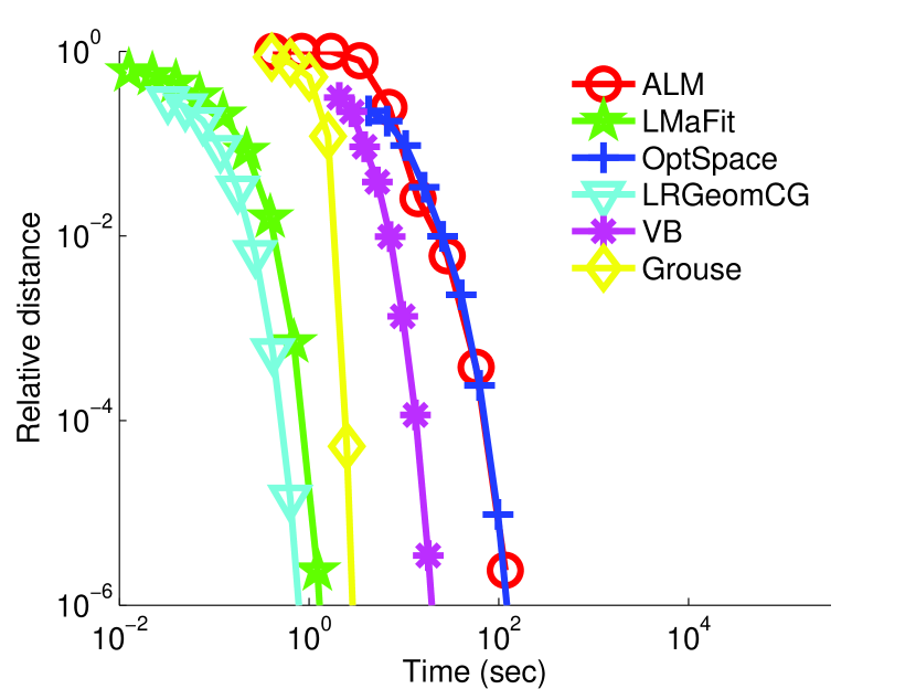
(a) $\mbox{OS}=6$, $r=20$, $\sigma=0$

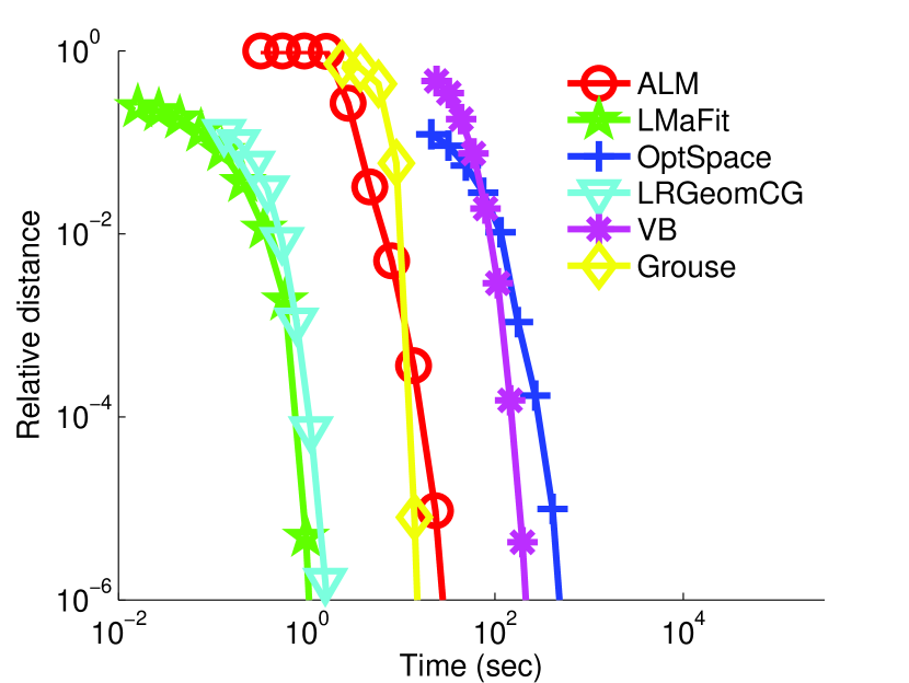
(b) $\mbox{OS}=6$, $r=50$, $\sigma=0$

(c) $\mbox{OS}=6$, $r=50$, $\sigma=0.1$

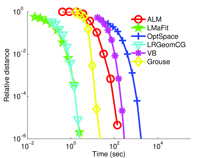
(d) $\mbox{OS}=3$, $r=50$, $\sigma=0$

Figure 1: Comparison of algorithms for matrix completion. Each curve represents the relative distance between an algorithm estimate and the true low-rank matrix as a function of time on a $\log_{10}/\log_{10}$ scale. The problem size is fixed as $1000\times 1000$. OS, $r$ and $\sigma$ denote the over-sampling ratio, the true rank and the noise level, respectively.

4.2 RPCA

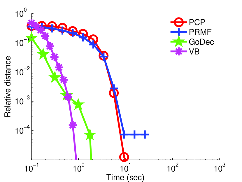
(a). $\rho=0.1$, $r=20$, $\sigma=0$

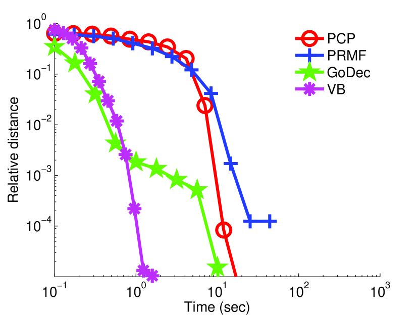
(b). $\rho=0.1$, $r=50$, $\sigma=0$

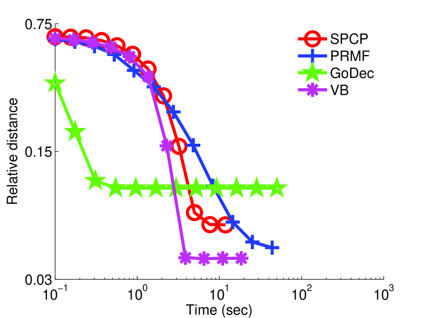
(c). $\rho=0.1$, $r=50$, $\sigma=0.1$

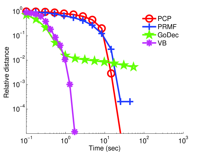
(d). $\rho=0.3$, $r=50$, $\sigma=0$

Figure 2: Comparison of algorithms for RPCA. Each curve represents the relative distance between an algorithm estimate and the true low-rank matrix as a function of time on a $\log_{10}/\log_{10}$ scale. The problem size is fixed to be $1000\times 1000$. $\rho$, $r$ and $\sigma$ denote the proportion of outlier entries, the true rank and the noise level, respectively.

The problem settings for RPCA are similar to the settings for matrix completion. The proportion of outliers is defined as $\rho=|\Omega|/mn$. A larger $\rho$ indicates more outliers, which makes the recovery more difficult. The results are shown in Figure 2.

The convex program PCP achieves a very high accuracy in noiseless cases without knowing the true rank. For the noisy case, its stable version SPCP is tested, which does not obtain the best accuracy due to the shrinkage effect of nuclear norm minimization as mentioned in the previous subsection. The probabilistic method PRMF achieves similar performance to PCP. Another probabilistic method VB using the Variational Bayes inference achieves the best overall performance in terms of both speed and accuracy, and it requires no parameter tuning. The projection-based method GoDec performs very well under the first two cases, but the performance drops in the more difficult cases in Figure 2(c) and (d), where the curves are flattened at high values.

5 Applications in Image Analysis

Many objects of interest in image analysis can be modeled as low-rank matrices, such as the images of a convex lambertian surface under various illuminations (Basri and Jacobs, 2003), dynamic textures changing periodically (Doretto et al., 2003), active contours with similar shapes (Blake and Isard, 2000), and multiple feature tracks on a rigid moving object (Vidal and Hartley, 2004). Intuitively, the low-dimensional subspace models the common patterns underlying the data. Hence, recovering the low-rank structure is critical to many applications such as background subtraction, face recognition, and segmentation. Below, we will introduce some typical applications based on the models we have discussed in the previous sections.

5.1 Face Recognition

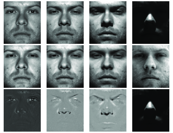
Figure 3: Using RPCA to remove shadows and specularities in face images. The rows from top to bottom correspond to the original images, the low-rank components and the sparse components, respectively. We applied the PCP algorithm (Candès et al., 2011) on a set of 64 face images of a person and selected 4 images to show the results. Note that the displayed intensities in each image have been scaled to [0, 255]. Face image courtesy of the Extended Yale Face Database B (Georghiades et al., 2001; Lee et al., 2005).

The concept of low dimensionality has been used in face recognition for decades since the work by Sirovich and Kirby (1987). PCA was applied on a set of face images to construct a face space and each face image can be characterized by a low-dimensional vector (Sirovich and Kirby, 1987; Kirby and Sirovich, 1990). Later on, Turk and Pentland (1991) introduced the “eigenface” method for face recognition. The basic steps of using eigenfaces for face recognition include: (1) generating $N$ eigenfaces by computing the first $N$ eigenvectors of the matrix composed of a set of training images; (2) calculating the weight vector of an input image by projecting the image onto the space spanned by the $N$ eigenfaces; and (3) determining whether the input image is a face image and if so, which person the image belongs to according to the projection error and the weight vector. This is the earliest example of using low-rank modeling for face recognition.

The face images in real datasets are usually corrupted by various artifacts such as shadows, specularities and occlusions, which cannot be handled by classical PCA. Therefore, many approaches based on RPCA were proposed to process face images (De La Torre and Black, 2003; Candès et al., 2011; Chen et al., 2012). As illustrated in Figure 3, the local defects in face images could be removed as the sparse component, while the correct description of the person’s face could be obtained from the low-rank component. This procedure can improve the characterization of faces and boost the performance of recognition algorithms (Chen et al., 2012).

5.2 Background Subtraction

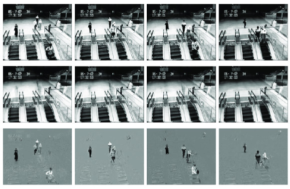
Figure 4: Using RPCA for background subtraction. The rows from top to bottom correspond to the input images, the low-rank components (background) and the sparse components (foreground), respectively. We applied the PCP algorithm (Candès et al., 2011) on the subway station dataset from Li et al. (2004). The dataset (used with permission of Liyuan Li) is a surveillance video of a subway station including moving escalators in the background. We selected 200 frames to perform background subtraction and 4 frames to show the results in the figure.

Background subtraction involves modeling the background in a video and detecting the objects that stand out from the background. Similar to eigenfaces, PCA has been applied to model the background since the work “eigenbackground subtraction” (Oliver et al., 2000). The basic idea is that the underlying background images of a video captured by a static camera should be unchanged except for illumination variation. Therefore, the matrix composed of vectorized background images can be naturally modeled as a low-rank matrix. However, a set of training images without foreground objects are required to generate a clean background model in traditional methods. To estimate a background model at the presence of foreground objects, RPCA is desired (De La Torre and Black, 2003). As illustrated in (Candès et al., 2011), the PCP algorithm can recover the background images in the low-rank component and identify the foreground objects in the sparse component. Figure 4 gives an illustration. Notice that the background includes three moving escalators, which are clearly reconstructed in the low-rank component. This shows the appealing capability of low-rank modeling for background subtraction. To achieve better accuracy for object detection, the spatially-contiguous property of foreground pixels can be modeled and integrated into RPCA by using Markov Random Fields or other smoothing techniques (Zhou et al., 2013b; Gao et al., 2012; Wang and Yeung, 2013). Similarly, the RPCA framework can be used to segment the point trajectories in a video into two groups, which correspond to background and foreground, respectively (Cui et al., 2012). The segmentation is based on the fact that the background motion caused by camera motion should lie in a low-dimensional subspace.

5.3 Clustering and Classification

Low-Rank Representation (LRR) is a well known method for subspace clustering. In subspace clustering, the data points are assumed to be embedded in several low-dimensional subspaces, and the task is to find these subspaces and the membership of each data point in these subspaces. A popular method is spectral clustering, where the clustering is achieved by partitioning a graph whose edge weight represents the affinity between two data points. In LRR, each data point is represented by a linear combination of its neighbors within the same subspace, and the coefficient ${\mathbf{X}}$ is estimated by

$$\min_{{\mathbf{X}},{\mathbf{E}}}~{} \|{\mathbf{X}}\|_{*}+\lambda\|{\mathbf{E}}\|_{2,1},$$

s.t. $${\mathbf{D}}={\mathbf{D}}{\mathbf{X}}+{\mathbf{E}},$$ (50)

where $\|{\mathbf{E}}\|_{2,1}=\sum_{j}\sqrt{\sum_{i}E_{ij}^{2}}$ encourages column-wise sparsity on the outlier term ${\mathbf{E}}$. It can be shown that, if the data points in ${\mathbf{D}}$ are from several orthogonal subspaces, ${\mathbf{X}}$ derived from (5.3) will be block-diagonal (Liu et al., 2010). Intrinsically, ${\mathbf{X}}$ identifies the affinity between data points, and its block-diagonal structure indicates clusters in the data. Thus, ${\mathbf{X}}$ provides a favorable affinity matrix to perform spectral clustering. A similar idea has also been applied to image segmentation Cheng et al. (2011).

Another application of low-rank representation is on dictionary learning for image classification. In dictionary learning, the primary task is to construct a dictionary ${\mathbf{\Phi}}=[\phi_{i},\cdots,\phi_{n}]$, such that the input signals can be represented by sparse linear combinations of dictionary atoms. That is, ${\mathbf{D}}={\mathbf{\Phi}}{\mathbf{X}}+{\mathbf{E}}$, where ${\mathbf{X}}$ should be sparse. In (Zhang et al., 2012b, 2013b, 2013c), it has been claimed that ${\mathbf{X}}$ should also be low-rank to learn a discriminative dictionary. The intuition is that, if the constructed dictionary ${\mathbf{\Phi}}$ is discriminative, the signals in ${\mathbf{D}}$ with the same label should be represented by the same set of atoms in ${\mathbf{\Phi}}$. Consequently, the coefficient matrix ${\mathbf{X}}$ should be a block-diagonal matrix if the columns are ordered by class labels. To impose such a structural constraint, the sparsity and the rank of ${\mathbf{X}}$ are minimized simultaneously.

5.4 Image Alignment and Rectification

Image alignment refers to the problem of transforming different images into the same coordinate system. Peng et al. (2012) proposed to solve the problem by rank minimization based on the assumption that a batch of aligned images should form a low-rank matrix. The parameters of transformation $\tau$ were estimated by solving

$$\min_{\tau,{\mathbf{X}},{\mathbf{E}}}~{} \|{\mathbf{X}}\|_{*}+\lambda\|{\mathbf{E}}\|_{1},$$

s.t. $${\mathbf{X}}+{\mathbf{E}}={\mathbf{D}}\circ\tau,$$ (51)

where each column of ${\mathbf{D}}$ corresponds to an image to be aligned and ${\mathbf{D}}\circ\tau$ denotes the images after transformation. The sparse component ${\mathbf{E}}$ models local differences among images.

Similarly, Zhang et al. (2012c) used the model in (5.4) to generate transform-invariant low-rank textures (TILT). The difference compared to (Peng et al., 2012) is that ${\mathbf{D}}$ in TILT represents a single image instead of an image sequence. The assumption of TILT is that the rectified images of textures such as characters, bar codes and urban scenes are usually symmetric patterns and consequently form low-rank matrices. The reconstructed low-rank texture can be further used in many applications such as camera calibration, 3D reconstruction, character recognition, etc.

5.5 Structure and Motion

The low-rank matrix factorization has been widely used to analyze the tracks of feature points in a video since the seminal work by Tomasi and Kanade (1992). The key observation is that a measurement matrix composed of feature tracks will be rank-limited and the rank depends on the type of camera model (e.g. affine or perspective) and the complexity of object motion (e.g. rigid or non-rigid). For example, under the weak-perspective model, the 2D image coordinates ${\mathbf{x}}\in\mathbb{R}^{2}$ and the 3D position $X\in\mathbb{R}^{3}$ of a feature point are related by the following equation:

$${\mathbf{x}}={\mathbf{M}}\left[\begin{array}[]{c}X\\ 1\\ \end{array}\right],$$ (54)

where ${\mathbf{M}}\in\mathbb{R}^{2\times 4}$ is an affine motion matrix. If a set of feature points on a rigid object are tracked across many frames, we have

$$\underbrace{\left[\begin{array}[]{ccc}{\mathbf{x}}_{11}&\cdots&{\mathbf{x}}_{1n}\\ \vdots&\ddots&\vdots\\ {\mathbf{x}}_{m1}&\cdots&{\mathbf{x}}_{mn}\\ \end{array}\right]}_{{\mathbf{P}}\in\mathbb{R}^{2m\times n}}=\underbrace{\left[\begin{array}[]{c}{\mathbf{M}}_{1}\\ \vdots\\ {\mathbf{M}}_{m}\\ \end{array}\right]}_{{\mathbf{M}}\in\mathbb{R}^{2m\times 4}}\underbrace{\left[\begin{array}[]{ccc}X_{1}&\cdots&X_{n}\\ 1&\cdots&1\\ \end{array}\right]}_{{\mathbf{S}}\in\mathbb{R}^{4\times n}},$$ (63)

where ${\mathbf{x}}_{ij}$ denotes the 2D image coordinates of point $j$ in frame $i$, ${\mathbf{M}}_{i}$ is the affine motion matrix for frame $i$, and $X_{j}$ is the 3D coordinates of point $j$. ${\mathbf{P}}$, ${\mathbf{M}}$ and ${\mathbf{S}}$ are often called measurement matrix, motion matrix and structure matrix, respectively (Tomasi and Kanade, 1992). Since the smallest dimension of ${\mathbf{M}}$ is 4, we have $\mbox{rank}({\mathbf{P}})\leq 4$. In addition, it is possible to recover the structure and motion matrices from the low-rank factorization of the measurement matrix in (63), which solves the problem of structure from motion (SFM) Tomasi and Kanade (1992). For nonrigid SFM, the object shape changes from frame to frame, and (63) is only valid for each frame separately with $m=1$, which is an undetermined system. To make the problem well posed, prior knowledge on the shapes is required. The low-rank prior is widely adopted by many state-of-the-art methods for nonrigid SFM, which assumes that the shapes to be reconstructed are linear combinations of a limited number of basis shapes. Exemplar works include (Bregler et al., 2000; Xiao et al., 2006; Angst et al., 2011; Dai et al., 2012).

Given that the measurement matrix itself is low-rank, the low-rank constraint can also be used to help tracking feature points and finding correspondences across video frames (Torresani and Bregler, 2002; Irani, 2002; Garg et al., 2013).

Another related application is motion segmentation (Vidal and Ma, 2004; Rao et al., 2010; Vidal, 2011), where the feature tracks are from multiple moving objects instead of a single rigid object. The task is to segment the feature tracks into different groups, and each group of tracks belong to a single moving object. As discussed above, each group of tracks should form a rank-4 subspace. Therefore, the motion segmentation problem can be formulated as subspace clustering, i.e. dividing the feature tracks into multiple clusters with each cluster forming a low-dimensional subspace. For a more detailed introduction to subspace clustering, please refer to (Vidal, 2011).

5.6 Restoration and Denoising

A popular application of matrix completion is image restoration. In many scenarios, it is desired to reconstruct the lost or corrupted parts of an image, which might be caused by texts or logos superposed on the image. This process is named image restoration or inpainting (Bertalmio et al., 2000). As a natural image is approximately low-rank (Zhang et al., 2012a), the problem of restoring the corrupted pixels can be formulated as a matrix completion problem. Figure 5 is an illustration of using matrix completion to restore an image from randomly sampled pixels or a text-occluded image. Liang et al. (2012) used a more sophisticated model, where the texture to be recovered is modeled as both low-rank and sparse in a certain transformed domain. Moreover, they assumed that the corrupted regions might be unknown and used a sparse error term to model and detect the corrupted regions. To alleviate the shrinkage of signals, some works adopted nonconvex methods for rank minimization instead of using the nuclear norm (Zhang et al., 2012a; Gu et al., 2014). Ji et al. (2010) proposed a method for video restoration. The unreliable pixels in the video are first detected and labeled as missing. Then, the image patches are grouped such that the patches in each group share a similar underlying structure and approximately form a low-rank matrix. Finally, the matrix completion is carried out on each patch group to restore the images.

Similarly, the low-rank assumption is often used to model the coherence of multiple images for noise removal in medical image analysis. In denoising of magnetic resonance (MR) images, for example, an image sequence usually consists of multiple echo images Bydder and Du (2006), frames of dynamic imaging Nguyen et al. (2011) or different diffusion-weighted images Lam et al. (2012). Although the images are different, the desired signals in these images are supposed to be correlated and consequently can be reconstructed with several significant principal components. The remaining components correspond to random noise, which are removed. Recently, Candes et al. (2013) used the SVT operator in (11) instead of classical PCA to achieve more robust results for image denoising. More importantly, it has been shown that the optimal threshold for SVT can be obtained theoretically based on the Stein’s unbiased risk estimate (Candes et al., 2013), which brings great convenience to practical applications.

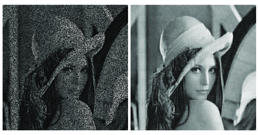
(a)

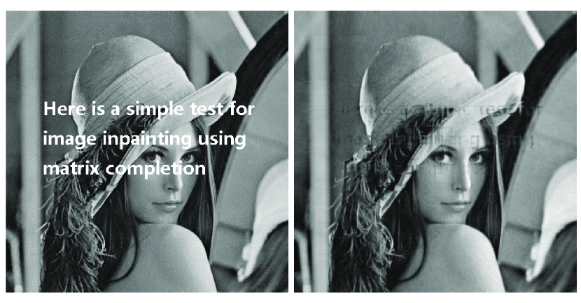
(b)

Figure 5: Matrix completion for image restoration. (a) The input image with $50\%$ missing pixels and the recovered image. (b) The input image corrupted by text and the recovered image. The SOFT-IMPUTE (Mazumder et al., 2010) algorithm was applied. Original image from http://en.wikipedia.org/wiki/File:Lenna.png.

5.7 Image Segmentation

The active shape model (Cootes et al., 1995) was proposed to increase the robustness of deformable models for image segmentation. It constructs a statistical shape space from a large set of given shapes and constrains the candidate shape in the shape space. In the active shape model, a candidate shape is represented as

$$\mathcal{C}({\mathbf{w}})=\overline{\mathcal{C}}+{\mathbf{\Phi}}{\mathbf{w}},$$ (64)

where $\overline{\mathcal{C}}$ denotes the mean shape, ${\mathbf{\Phi}}$ is a matrix consisting of vectors describing shape variations in the training data, and ${\mathbf{w}}$ is a vector of coefficients to represent the candidate shape in the shape space. Then, ${\mathbf{w}}$ is determined by fitting the parametric curve in (64) to the features in the image. Since the number of columns of ${\mathbf{\Phi}}$ is often small, the candidate shape is confined in a low-dimensional space. Therefore, the active shape model intrinsically admits a low-rank assumption on the population of shapes. Moreover, $\overline{\mathcal{C}}$ and ${\mathbf{\Phi}}$ are derived by applying PCA to the set of training shapes. The active shape model was later extended to the active appearance model to make use of both shape and appearance information (Cootes et al., 2001). More exemplar methods building upon the active shape model for image segmentation include (Leventon et al., 2000; Tsai et al., 2001; Cremers, 2006; Zhu et al., 2010). An alternative approach to making use of the low-rank assumption for image segmentation is to impose a group-similarity constraint on multiple shapes by nuclear norm minimization (Zhou et al., 2013a), which does not require training shapes.

5.8 Medical Image Reconstruction

Image reconstruction based on low-rank modeling has drawn much attention in the medical imaging community. The idea is to make use of the temporal coherence in dynamic imaging to reduce the required number of sampling. In MR imaging, for example, Liang (2007) proposed the concept of partial separability (PS) to model a spatial-temporal MR image $\rho({\mathbf{x}},t)$ as

$$\rho({\mathbf{x}},t)=\sum_{\ell=1}^{L}{\phi_{\ell}({\mathbf{x}})v_{\ell}(t)},$$ (65)

where $\phi_{\ell}({\mathbf{x}})$ and $v_{\ell}(t)$ for $\ell=1,\cdots,L$ are spatial and temporal components, respectively. $L$ is the order of the model. Correspondingly, any sample in the $({\mathbf{k}},t)$-space can be expressed as $c({\mathbf{k}},t)=\sum_{\ell=1}^{L}{u_{\ell}({\mathbf{k}})v_{\ell}(t)}$, where $u_{\ell}({\mathbf{k}})$ is the Fourier transform of $\phi_{\ell}({\mathbf{x}})$. Using matrix notations, we have

$${\mathbf{C}}={\mathbf{U}}{\mathbf{V}},$$ (66)

where $C_{ij}=c({\mathbf{k}}_{i},t_{j})$, $U_{i\ell}=u_{\ell}({\mathbf{k}}_{i})$ and $V_{\ell j}=v_{\ell}(t_{j})$. Since the images are temporally coherent, $L$ can be very small, which gives a low-rank model of the coefficients ${\mathbf{C}}$ in the $({\mathbf{k}},t)$-space. Hence, a small number of samples are sufficient to estimate ${\mathbf{C}}$ and reconstruct the image sequence. For example, $u_{\ell}({\mathbf{k}})$ and $v_{\ell}(t)$ for $\ell=1,\cdots,L$ can be computed by fully sampling $L$ columns and rows of the $({\mathbf{k}},t)$-space (Liang, 2007). Some works used other sampling schemes and solved the reconstruction problem by matrix recovery algorithms (Haldar and Liang, 2010, 2011).

The basic PS model can be further extended to integrate other sparse properties in specific domains. For example, the image intensity $\phi_{\ell}({\mathbf{x}})$ often has a sparse representation in wavelets or a limited total variation (Lustig et al., 2008; Lingala et al., 2011; Majumdar and Ward, 2012). Meanwhile, the temporal component $v_{\ell}(t)$ is usually periodic or bandlimited, which results in sparsity in the Fourier domain (Zhao et al., 2010, 2012). The low-rank property is modeled as regionally dependent and exploited locally in (Christodoulou et al., 2012; Trzasko, 2013). Instead of using the PS model, some works (Lingala et al., 2011; Majumdar and Ward, 2012) proposed to reconstruct data by nuclear norm minimization. Otazo et al. (2013) used a RPCA model to separate background and dynamic components in imaging. Lingala and Jacob (2013) developed a dictionary learning-based framework for dynamic imaging. Low-rank modeling has also been applied to reconstruct multi-channel data (Shin et al., 2013), single ${\mathbf{k}}$-space data (Haldar, 2014) and imaging data from other modalities such as computed tomography (CT) (Cai et al., 2014; Gao et al., 2011) and positron emission tomography (PET) (Rahmim et al., 2009).

5.9 More Applications

Recent examples of low-rank modeling-based applications also include object tracking (Ross et al., 2008; Zhang et al., 2012b), saliency detection (Shen and Wu, 2012), correspondence estimation (Zeng et al., 2012; Chen et al., 2014), façade parsing (Yang et al., 2012), model fusion (Ye et al., 2012; Pan et al., 2013), and depth image enhancement (Shu et al., 2014), to name a few.

6 Discussions

In this paper, we have introduced the concept of low-rank modeling and reviewed some representative low-rank models, algorithms and applications in image analysis. For additional reading on theories, algorithms and applications, the readers are referred to online documents such as the Matrix Factorization Jungle and the Sparse and Low-rank Approximation Wiki, which are updated on a regular basis.

The convex programming-based methods for low-rank matrix recovery generally achieve a stable performance under a wide range of scenarios due to the global optimality in optimization. In noiseless cases, the convex programs such as (2.1) and (2.2) can exactly recover the underlying low-rank matrix with a theoretical guarantee (Candès and Recht, 2009; Candès et al., 2011). In noisy cases, the nuclear norm minimization may shrink true signals while compressing noise. To compensate for the shrinkage effect, some postprocessing steps may be used (Mazumder et al., 2010), while some other works tried to alleviate this issue by going beyond the nuclear norm and using nonconvex relaxation techniques (Mohan and Fazel, 2012; Zhang et al., 2012a). A limitation of convex methods is the requirement of repeated SVD computation, which is time consuming and unaffordable in large-scale problems. While many efforts have been made towards fast SVD computation such as partial SVD (Lin et al., 2010), approximate SVD (Ma et al., 2011) or performing SVT without SVD (Cai and Osher, 2010), computational efficiency is still an issue in many real applications.

The factorization-based methods are widely used in real applications (e.g. building recommender systems (Koren et al., 2009)), mostly due to the computational convenience. Inference of a large matrix is reduced to estimation of two smaller factor matrices. Moreover, the cost function of matrix factorization is often decomposable as a sum of separate functions over data points or variables. Therefore, it is convenient to develop online algorithms for real-time processing and to design distributed algorithms for solving large-scale problems. A limitation of matrix factorization is that the underlying rank needs to be predefined in many models. While rank estimation techniques have been proposed in some works such as (Keshavan et al., 2009) and (Wen et al., 2012), rank estimation is still a challenging problem especially in noisy cases. The probabilistic methods have shown great potential in both simulation (Babacan et al., 2012) and real application (Wang and Yeung, 2013). Moreover, the probabilistic models with a Bayesian treatment are often parameter free, which is important in real applications.

The applications of low-rank modeling are based on the fact that linear correlation often exists among data. Such prior knowledge can be used for many purposes such as extracting common patterns, removing random noise, reducing sampling rates in imaging, etc. The recent advances in sparse learning and optimization provide powerful frameworks and techniques to conveniently model the low-rank property of data and develop efficient algorithms. We expect to see more applications of low-rank modeling in the near future.

References

- Aanæs et al. [2002] H. Aanæs, R. Fisker, K. Astrom, and J. M. Carstensen. Robust factorization. IEEE Transactions on Pattern Analysis and Machine Intelligence, 24(9):1215–1225, 2002.
- Absil et al. [2013] P.-A. Absil, L. Amodei, and G. Meyer. Two newton methods on the manifold of fixed-rank matrices endowed with riemannian quotient geometries. Computational Statistics, pages 1–22, 2013.
- Angst et al. [2011] R. Angst, C. Zach, and M. Pollefeys. The generalized trace-norm and its application to structure-from-motion problems. In Proceedins of International Conference on Computer Vision, 2011.
- Babacan et al. [2012] S. D. Babacan, M. Luessi, R. Molina, and A. K. Katsaggelos. Sparse Bayesian methods for low-rank matrix estimation. IEEE Transactions on Signal Processing, 60(8):3964–3977, 2012.
- Balzano et al. [2010] L. Balzano, R. Nowak, and B. Recht. Online identification and tracking of subspaces from highly incomplete information. In Proceedings of Annual Allerton Conference on Communication, Control, and Computing, 2010.
- Basri and Jacobs [2003] R. Basri and D. Jacobs. Lambertian reflectance and linear subspaces. IEEE Transactions on Pattern Analysis and Machine Intelligence, 25(2):218–233, 2003.
- Beck and Teboulle [2009] A. Beck and M. Teboulle. A fast iterative shrinkage-thresholding algorithm for linear inverse problems. SIAM Journal on Imaging Sciences, 2(1):183–202, 2009.
- Bertalmio et al. [2000] M. Bertalmio, G. Sapiro, V. Caselles, and C. Ballester. Image inpainting. In Proceedings of Annual Conference on Computer Graphics and Interactive Techniques, 2000.
- Bertsekas [1999] D. Bertsekas. Nonlinear programming. Athena Scientific, 1999.
- Bishop [1999] C. M. Bishop. Bayesian PCA. In Advances in Neural Information Processing Systems, pages 382–388, 1999.
- Bishop et al. [2006] C. M. Bishop et al. Pattern recognition and machine learning. Springer New York, 2006.
- Blake and Isard [2000] A. Blake and M. Isard. Active contours. Springer, 2000.
- Blumensath and Davies [2009] T. Blumensath and M. E. Davies. Iterative hard thresholding for compressed sensing. Applied and Computational Harmonic Analysis, 27(3):265–274, 2009.
- Boumal and Absil [2011] N. Boumal and P.-A. Absil. RTRMC: A Riemannian trust-region method for low-rank matrix completion. In Advances in Neural Information Processing Systems, pages 406–414, 2011.
- Boumal et al. [2014] N. Boumal, B. Mishra, P.-A. Absil, and R. Sepulchre. Manopt, a matlab toolbox for optimization on manifolds. Journal of Machine Learning Research, 15:1455–1459, 2014.
- Boyd [2010] S. Boyd. Distributed optimization and statistical learning via the alternating direction method of multipliers. Foundations and Trends in Machine Learning, 3(1):1–122, 2010.
- Brand [2002] M. Brand. Incremental singular value decomposition of uncertain data with missing values. In Proceedings of the European Conference on Computer Vision, 2002.
- Bregler et al. [2000] C. Bregler, A. Hertzmann, and H. Biermann. Recovering non-rigid 3d shape from image streams. In Proceedings of the IEEE Conference on Computer Vision and Pattern Recognition, 2000.
- Buchanan and Fitzgibbon [2005] A. M. Buchanan and A. W. Fitzgibbon. Damped newton algorithms for matrix factorization with missing data. In Proceedings of the IEEE Conference on Computer Vision and Pattern Recognition, 2005.
- Bunch and Nielsen [1978] J. R. Bunch and C. P. Nielsen. Updating the singular value decomposition. Numerische Mathematik, 31(2):111–129, 1978.
- Bydder and Du [2006] M. Bydder and J. Du. Noise reduction in multiple-echo data sets using singular value decomposition. Magnetic Resonance Imaging, 24(7):849–856, 2006.
- Cabral et al. [2013] R. Cabral, F. De la Torre, J. P. Costeira, and A. Bernardino. Unifying nuclear norm and bilinear factorization approaches for low-rank matrix decomposition. In Proceedings of the International Conference on Computer Vision, 2013.
- Cai and Osher [2010] J. Cai and S. Osher. Fast singular value thresholding without singular value decomposition. UCLA CAM Report, 5, 2010.
- Cai et al. [2010] J. Cai, E. Candès, and Z. Shen. A singular value thresholding algorithm for matrix completion. SIAM Journal on Optimization, 20:1956, 2010.
- Cai et al. [2014] J. Cai, X. Jia, H. Gao, S. Jiang, Z. Shen, and H. Zhao. Cine cone beam CT reconstruction using low-rank matrix factorization: algorithm and a proof-of-princple study. IEEE Transactions on Medical Imaging, 33(8):1581–1591, 2014.
- Candes and Plan [2010] E. Candes and Y. Plan. Matrix completion with noise. Proceedings of the IEEE, 98(6):925–936, 2010.
- Candès and Recht [2009] E. Candès and B. Recht. Exact matrix completion via convex optimization. Foundations of Computational Mathematics, 9(6):717–772, 2009.
- Candès et al. [2011] E. Candès, X. Li, Y. Ma, and J. Wright. Robust principal component analysis? Journal of the ACM, 58(3):11, 2011.
- Candes et al. [2013] E. Candes, C. Sing-Long, and J. Trzasko. Unbiased risk estimates for singular value thresholding and spectral estimators. IEEE Transactions on Signal Processing, 61(19):4643–4657, 2013.
- Candès and Tao [2010] E. J. Candès and T. Tao. The power of convex relaxation: Near-optimal matrix completion. IEEE Transactions on Information Theory, 56(5):2053–2080, 2010.
- Chandrasekaran et al. [2011] V. Chandrasekaran, S. Sanghavi, P. Parrilo, and A. Willsky. Rank-sparsity incoherence for matrix decomposition. SIAM Journal on Optimization, 21(2):572–596, 2011.
- Chen et al. [2012] C. Chen, C. Wei, and Y. Wang. Low-rank matrix recovery with structural incoherence for robust face recognition. In Proceedings of the IEEE Conference on Computer Vision and Pattern Recognition, 2012.
- Chen [2008] P. Chen. Optimization algorithms on subspaces: Revisiting missing data problem in low-rank matrix. International Journal of Computer Vision, 80(1):125–142, 2008.
- Chen et al. [2014] Y. Chen, L. Guibas, and Q. Huang. Near-optimal joint object matching via convex relaxation. In Proceedings of the International Conference on Machine Learning, 2014.
- Cheng et al. [2011] B. Cheng, G. Liu, J. Wang, Z. Huang, and S. Yan. Multi-task low-rank affinity pursuit for image segmentation. In Proceedings of the International Conference on Computer Vision, 2011.
- Christodoulou et al. [2012] A. Christodoulou, S. Babacan, and Z. Liang. Accelerating cardiovascular imaging by exploiting regional low-rank structure via group sparsity. In Proceedings of the IEEE International Symposium on Biomedical Imaging, 2012.
- Comon and Golub [1990] P. Comon and G. H. Golub. Tracking a few extreme singular values and vectors in signal processing. Proceedings of the IEEE, 78(8):1327–1343, 1990.
- Cootes et al. [1995] T. Cootes, C. Taylor, D. Cooper, and J. Graham. Active shape models – their training and application. Computer Vision and Image Understanding, 61(1):38–59, 1995.
- Cootes et al. [2001] T. F. Cootes, G. J. Edwards, and C. J. Taylor. Active appearance models. IEEE Transactions on Pattern Analysis and Machine Intelligence, 23(6):681–685, 2001.
- Cremers [2006] D. Cremers. Dynamical statistical shape priors for level set-based tracking. IEEE Transactions on Pattern Analysis and Machine Intelligence, 28(8):1262–1273, 2006.
- Cui et al. [2012] X. Cui, J. Huang, S. Zhang, and D. N. Metaxas. Background subtraction using low rank and group sparsity constraints. In Proceedings of the European Conference on Computer Vision, 2012.
- Dai et al. [2011] W. Dai, O. Milenkovic, and E. Kerman. Subspace evolution and transfer (SET) for low-rank matrix completion. IEEE Transactions on Signal Processing, 59(7):3120–3132, 2011.
- Dai et al. [2012] Y. Dai, H. Li, and M. He. A simple prior-free method for non-rigid structure-from-motion factorization. In Proceedings of the IEEE Conference on Computer Vision and Pattern Recognition, 2012.
- De La Torre and Black [2003] F. De La Torre and M. Black. A framework for robust subspace learning. International Journal of Computer Vision, 54(1):117–142, 2003.
- Ding et al. [2011] X. Ding, L. He, and L. Carin. Bayesian robust principal component analysis. IEEE Transactions on Image Processing, 20(12):3419–3430, 2011.
- Doretto et al. [2003] G. Doretto, A. Chiuso, Y. Wu, and S. Soatto. Dynamic textures. International Journal of Computer Vision, 51(2):91–109, 2003.
- Eckart and Young [1936] C. Eckart and G. Young. The approximation of one matrix by another of lower rank. Psychometrika, 1(3):211–218, 1936.
- Edelman et al. [1998] A. Edelman, T. A. Arias, and S. T. Smith. The geometry of algorithms with orthogonality constraints. SIAM journal on Matrix Analysis and Applications, 20(2):303–353, 1998.
- Eriksson and Van Den Hengel [2010] A. Eriksson and A. Van Den Hengel. Efficient computation of robust low-rank matrix approximations in the presence of missing data using the l1 norm. In Proceedings of the IEEE Conference on Computer Vision and Pattern Recognition, 2010.
- Fazel [2002] M. Fazel. Matrix rank minimization with applications. PhD thesis, Stanford University, 2002.
- Gao et al. [2011] H. Gao, J. Cai, Z. Shen, and H. Zhao. Robust principal component analysis-based four-dimensional computed tomography. Physics in Medicine and Biology, 56(11):3181, 2011.
- Gao et al. [2012] Z. Gao, L. Cheong, and M. Shan. Block-sparse RPCA for consistent foreground detection. In Proceedings of the European Conference on Computer Vision, 2012.
- Garg et al. [2013] R. Garg, A. Roussos, and L. Agapito. A variational approach to video registration with subspace constraints. International Journal of Computer Vision, 104(3):286–314, 2013.
- Gemulla et al. [2011] R. Gemulla, E. Nijkamp, P. J. Haas, and Y. Sismanis. Large-scale matrix factorization with distributed stochastic gradient descent. In Proceedings of the International Conference on Knowledge Discovery and Data Mining, 2011.
- Georghiades et al. [2001] A. S. Georghiades, P. N. Belhumeur, and D. J. Kriegman. From few to many: Illumination cone models for face recognition under variable lighting and pose. IEEE Transactions on Pattern Analysis and Machine Intelligence, 23(6):643–660, 2001.
- Gross [2011] D. Gross. Recovering low-rank matrices from few coefficients in any basis. IEEE Transactions on Information Theory, 57(3):1548–1566, 2011.
- Gu et al. [2014] S. Gu, L. Zhang, W. Zuo, and X. Feng. Weighted nuclear norm minimization with application to image denoising. In Proceedings of the IEEE Conference on Computer Vision and Pattern Recognition, 2014.
- Haldar [2014] J. Haldar. Low-rank modeling of local k -space neighborhoods (loraks) for constrained MRI. IEEE Transactions on Medical Imaging, 33(3):668–681, March 2014.
- Haldar and Liang [2010] J. Haldar and Z. Liang. Spatiotemporal imaging with partially separable functions: A matrix recovery approach. In Proceedings of the IEEE International Symposium on Biomedical Imaging, 2010.
- Haldar and Liang [2011] J. Haldar and Z. Liang. Low-rank approximations for dynamic imaging. In Proceedings of the IEEE International Symposium on Biomedical Imaging, 2011.
- Haldar and Hernando [2009] J. P. Haldar and D. Hernando. Rank-constrained solutions to linear matrix equations using powerfactorization. IEEE Signal Processing Letters, 16(7):584–587, 2009.
- He et al. [2012] J. He, L. Balzano, and A. Szlam. Incremental gradient on the grassmannian for online foreground and background separation in subsampled video. In Proceedings of the IEEE Conference on Computer Vision and Pattern Recognition, 2012.
- Hotelling [1933] H. Hotelling. Analysis of a complex of statistical variables into principal components. The Journal of Educational Psychology, pages 498–520, 1933.
- Irani [2002] M. Irani. Multi-frame correspondence estimation using subspace constraints. International Journal of Computer Vision, 48(3):173–194, 2002.
- Jain et al. [2010] P. Jain, R. Meka, and I. S. Dhillon. Guaranteed rank minimization via singular value projection. In Proceedings of Advances in Neural Information Processing Systems, 2010.
- Jain et al. [2013] P. Jain, P. Netrapalli, and S. Sanghavi. Low-rank matrix completion using alternating minimization. In Proceedings of the annual ACM Symposium on theory of computing, 2013.
- Ji et al. [2010] H. Ji, C. Liu, Z. Shen, and Y. Xu. Robust video denoising using low rank matrix completion. In Proceedings of the IEEE Conference on Computer Vision and Pattern Recognition, 2010.
- Ji and Ye [2009] S. Ji and J. Ye. An accelerated gradient method for trace norm minimization. In Proceedings of the International Conference on Machine Learning, 2009.
- Jolliffe [2002] I. T. Jolliffe. Principal component analysis. Springer verlag, 2002.
- Ke and Kanade [2005] Q. Ke and T. Kanade. Robust l1 norm factorization in the presence of outliers and missing data by alternative convex programming. In Proceedings of the IEEE Conference on Computer Vision and Pattern Recognition, 2005.
- Keshavan et al. [2009] R. H. Keshavan, A. Montanari, and S. Oh. Low-rank matrix completion with noisy observations: a quantitative comparison. In Proceedings of Annual Allerton Conference on Communication, Control, and Computing, 2009.
- Keshavan et al. [2010a] R. H. Keshavan, A. Montanari, and S. Oh. Matrix completion from a few entries. IEEE Transactions on Information Theory, 56(6):2980–2998, 2010a.
- Keshavan et al. [2010b] R. H. Keshavan, A. Montanari, and S. Oh. Matrix completion from noisy entries. Journal of Machine Learning Research, 11(2057-2078):1, 2010b.
- Kirby and Sirovich [1990] M. Kirby and L. Sirovich. Application of the Karhunen-Loeve procedure for the characterization of human faces. IEEE Transactions on Pattern Analysis and Machine Intelligence, 12(1):103–108, 1990.
- Koren et al. [2009] Y. Koren, R. Bell, and C. Volinsky. Matrix factorization techniques for recommender systems. Computer, 42(8):30–37, 2009.
- Kwak [2008] N. Kwak. Principal component analysis based on l1-norm maximization. IEEE Transactions on Pattern Analysis and Machine Intelligence, 30(9):1672–1680, 2008.
- Lakshminarayanan et al. [2011] B. Lakshminarayanan, G. Bouchard, and C. Archambeau. Robust Bayesian matrix factorisation. In International Conference on Artificial Intelligence and Statistics, pages 425–433, 2011.
- Lam et al. [2012] F. Lam, S. Babacan, J. Haldar, N. Schuff, and Z. Liang. Denoising diffusion-weighted MR magnitude image sequences using low rank and edge constraints. In Proceedings of the IEEE International Symposium on Biomedical Imaging, 2012.
- Lawrence [2005] N. Lawrence. Probabilistic non-linear principal component analysis with Gaussian process latent variable models. The Journal of Machine Learning Research, 6:1783–1816, 2005.
- Lee and Seung [1999] D. Lee and H. Seung. Learning the parts of objects by non-negative matrix factorization. Nature, 401(6755):788, 1999.
- Lee and Bresler [2010] K. Lee and Y. Bresler. Admira: Atomic decomposition for minimum rank approximation. IEEE Transactions on Information Theory, 56(9):4402–4416, 2010.
- Lee et al. [2005] K. Lee, J. Ho, and D. Kriegman. Acquiring linear subspaces for face recognition under variable lighting. IEEE Transactions on Pattern Analysis and Machine Intelligence, 27(5):684–698, 2005.
- Leventon et al. [2000] M. Leventon, W. Grimson, and O. Faugeras. Statistical shape influence in geodesic active contours. In Proceedings of the IEEE Conference on Computer Vision and Pattern Recognition, 2000.
- Li et al. [2004] L. Li, W. Huang, I. Gu, and Q. Tian. Statistical modeling of complex backgrounds for foreground object detection. IEEE Transactions Image Processing, 13(11):1459–1472, 2004.
- Li et al. [2014] Y. Li, Y. Zhang, and Z. Huang. A reweighted nuclear norm minimization algorithm for low rank matrix recovery. Journal of Computational and Applied Mathematics, 263:338–350, 2014.
- Liang et al. [2012] X. Liang, X. Ren, Z. Zhang, and Y. Ma. Repairing sparse low-rank texture. In Proceedings of the European Conference on Computer Vision, 2012.
- Liang [2007] Z. Liang. Spatiotemporal imaging with partially separable functions. In Proceedings of the IEEE International Symposium on Biomedical Imaging, 2007.
- Lin et al. [2010] Z. Lin, M. Chen, and Y. Ma. The augmented Lagrange multiplier method for exact recovery of corrupted low-rank matrices. arXiv preprint arXiv:1009.5055, 2010.
- Lingala et al. [2011] S. Lingala, Y. Hu, E. DiBella, and M. Jacob. Accelerated dynamic MRI exploiting sparsity and low-rank structure: kt SLR. IEEE Transactions on Medical Imaging, 30(5):1042–1054, 2011.
- Lingala and Jacob [2013] S. G. Lingala and M. Jacob. Blind compressive sensing dynamic MRI. IEEE transactions on medical imaging, 32(6):1132–1145, 2013.
- Liu et al. [2010] G. Liu, Z. Lin, and Y. Yu. Robust subspace segmentation by low-rank representation. In Proceedings of the International Conference on Machine Learning, 2010.
- Lu et al. [2014] C. Lu, J. Tang, S. Y. Yan, and Z. Lin. Generalized nonconvex nonsmooth low-rank minimization. In Proceedings of the IEEE Conference on Computer Vision and Pattern Recognition, 2014.
- Lustig et al. [2008] M. Lustig, D. Donoho, J. Santos, and J. Pauly. Compressed sensing MRI. IEEE Signal Processing Magazine, 25(2):72–82, 2008.
- Ma et al. [2011] S. Ma, D. Goldfarb, and L. Chen. Fixed point and bregman iterative methods for matrix rank minimization. Mathematical Programming, 128(1-2):321–353, 2011.
- MacKay [1995] D. J. MacKay. Probable networks and plausible predictions-a review of practical Bayesian methods for supervised neural networks. Network: Computation in Neural Systems, 6(3):469–505, 1995.
- Mackey et al. [2011] L. W. Mackey, M. I. Jordan, and A. Talwalkar. Divide-and-conquer matrix factorization. In Advances in Neural Information Processing Systems, 2011.
- Majumdar and Ward [2012] A. Majumdar and R. Ward. Exploiting rank deficiency and transform domain sparsity for MR image reconstruction. Magnetic Resonance Imaging, 30(1):9–18, 2012.
- Majumdar and Ward [2011] A. Majumdar and R. K. Ward. An algorithm for sparse MRI reconstruction by schatten p-norm minimization. Magnetic resonance imaging, 29(3):408–417, 2011.
- Mallat and Zhang [1993] S. G. Mallat and Z. Zhang. Matching pursuits with time-frequency dictionaries. IEEE Transactions on Signal Processing, 41(12):3397–3415, 1993.
- Marjanovic and Solo [2012] G. Marjanovic and V. Solo. On lq optimization and matrix completion. IEEE Transactions on Signal Processing, 60(11):5714–5724, 2012.
- Markovsky [2012] I. Markovsky. Low rank approximation: algorithms, implementation, applications. Springer, 2012.
- Mazumder et al. [2010] R. Mazumder, T. Hastie, and R. Tibshirani. Spectral regularization algorithms for learning large incomplete matrices. The Journal of Machine Learning Research, 11:2287–2322, 2010.
- Meng and De la Torre [2013] D. Meng and F. De la Torre. Robust matrix factorization with unknown noise. In Proceedings of the International Conference on Computer Vision, 2013.
- Meyer et al. [2011] G. Meyer, S. Bonnabel, and R. Sepulchre. Linear regression under fixed-rank constraints: a riemannian approach. In Proceedings of the International Conference on Machine Learning, 2011.
- Michenková [2011] M. Michenková. Numerical algorithms for low-rank matrix completion problems, 2011.
- Mishra et al. [2012] B. Mishra, K. A. Apuroop, and R. Sepulchre. A riemannian geometry for low-rank matrix completion. arXiv preprint arXiv:1211.1550, 2012.
- Mishra et al. [2013a] B. Mishra, G. Meyer, F. Bach, and R. Sepulchre. Low-rank optimization with trace norm penalty. SIAM Journal on Optimization, 23(4):2124–2149, 2013a.
- Mishra et al. [2013b] B. Mishra, G. Meyer, S. Bonnabel, and R. Sepulchre. Fixed-rank matrix factorizations and riemannian low-rank optimization. Computational Statistics, 29:591–621, 2013b.
- Mohan and Fazel [2012] K. Mohan and M. Fazel. Iterative reweighted algorithms for matrix rank minimization. The Journal of Machine Learning Research, 13(1):3441–3473, 2012.
- Moreau [1965] J. Moreau. Proximité et dualité dans un espace hilbertien. Bulletin de la Société Mathématique de France, 93(2):273–299, 1965.
- Needell and Tropp [2009] D. Needell and J. A. Tropp. Cosamp: Iterative signal recovery from incomplete and inaccurate samples. Applied and Computational Harmonic Analysis, 26(3):301–321, 2009.
- Nesterov [1983] Y. Nesterov. A method of solving a convex programming problem with convergence rate . In Sov. Math., Dokl., volume 27, pages 372–376, 1983.
- Nesterov [2007] Y. Nesterov. Gradient methods for minimizing composite objective function. Technical report, Université catholique de Louvain, Center for Operations Research and Econometrics (CORE), 2007.
- Ngo and Saad [2012] T. Ngo and Y. Saad. Scaled gradients on grassmann manifolds for matrix completion. In Advances in Neural Information Processing Systems, 2012.
- Nguyen et al. [2011] H. Nguyen, X. Peng, M. Do, and Z. Liang. Spatiotemporal denoising of MR spectroscopic imaging data by low-rank approximations. In Proceedings of the IEEE International Symposium on Biomedical Imaging, 2011.
- Nie et al. [2012] F. Nie, H. Wang, X. Cai, H. Huang, and C. Ding. Robust matrix completion via joint schatten p-norm and lp-norm minimization. In Proceedings of the IEEE International Conference on Data Mining, 2012.
- O’Donoghue and Candes [2012] B. O’Donoghue and E. Candes. Adaptive restart for accelerated gradient schemes. Foundations of Computational Mathematics, pages 1–18, 2012.
- Okatani and Deguchi [2007] T. Okatani and K. Deguchi. On the Wiberg algorithm for matrix factorization in the presence of missing components. International Journal of Computer Vision, 72(3):329–337, 2007.
- Okatani et al. [2011] T. Okatani, T. Yoshida, and K. Deguchi. Efficient algorithm for low-rank matrix factorization with missing components and performance comparison of latest algorithms. In Proceedings of the International Conference on Computer Vision, 2011.
- Oliver et al. [2000] N. Oliver, B. Rosario, and A. Pentland. A Bayesian computer vision system for modeling human interactions. IEEE Transactions on Pattern Analysis and Machine Intelligence, 22(8):831–843, 2000.
- Otazo et al. [2013] R. Otazo, D. K. Sodickson, and E. J. Candès. Low-rank+ sparse (l+s) reconstruction for accelerated dynamic MRI with seperation of background and dynamic components. In Proceedings of the SPIE Optical Engineering + Applications, 2013.
- Pan et al. [2013] Y. Pan, H. Lai, C. Liu, and S. Yan. A divide-and-conquer method for scalable low-rank latent matrix pursuit. In Proceedings of the IEEE Conference on Computer Vision and Pattern Recognition, 2013.
- Peng et al. [2012] Y. Peng, A. Ganesh, J. Wright, W. Xu, and Y. Ma. RASL: Robust alignment by sparse and low-rank decomposition for linearly correlated images. IEEE Transactions on Pattern Analysis and Machine Intelligence, 34(11):2233–2246, 2012.
- Rahmim et al. [2009] A. Rahmim, J. Tang, and H. Zaidi. Four-dimensional (4D) image reconstruction strategies in dynamic PET: beyond conventional independent frame reconstruction. Medical physics, 36(8):3654–3670, 2009.
- Rao et al. [2010] S. Rao, R. Tron, R. Vidal, and Y. Ma. Motion segmentation in the presence of outlying, incomplete, or corrupted trajectories. IEEE Transactions on Pattern Analysis and Machine Intelligence, 32(10):1832–1845, 2010.
- Recht and Ré [2013] B. Recht and C. Ré. Parallel stochastic gradient algorithms for large-scale matrix completion. Mathematical Programming Computation, 5(2):201–226, 2013.
- Recht et al. [2010] B. Recht, M. Fazel, and P. Parrilo. Guaranteed minimum-rank solutions of linear matrix equations via nuclear norm minimization. SIAM Review, 52(3):471–501, 2010.
- Rennie and Srebro [2005] J. Rennie and N. Srebro. Fast maximum margin matrix factorization for collaborative prediction. In Proceedings of the International Conference on Machine learning, 2005.
- Ross et al. [2008] D. A. Ross, J. Lim, R.-S. Lin, and M.-H. Yang. Incremental learning for robust visual tracking. International Journal of Computer Vision, 77(1-3):125–141, 2008.
- Salakhutdinov and Mnih [2008a] R. Salakhutdinov and A. Mnih. Bayesian probabilistic matrix factorization using markov chain monte carlo. In Proceedings of the International Conference on Machine Learning, 2008a.
- Salakhutdinov and Mnih [2008b] R. Salakhutdinov and A. Mnih. Probabilistic matrix factorization. In Advances in Neural Information Processing Systems, 2008b.
- Shalit et al. [2012] U. Shalit, D. Weinshall, and G. Chechik. Online learning in the embedded manifold of low-rank matrices. The Journal of Machine Learning Research, 13:429–458, 2012.
- Shen and Wu [2012] X. Shen and Y. Wu. A unified approach to salient object detection via low rank matrix recovery. In Proceedings of the IEEE Conference on Computer Vision and Pattern Recognition, 2012.
- Shin et al. [2013] P. J. Shin, P. E. Larson, M. A. Ohliger, M. Elad, J. M. Pauly, D. B. Vigneron, and M. Lustig. Calibrationless parallel imaging reconstruction based on structured low-rank matrix completion. Magnetic Resonance in Medicine, 2013.
- Shu et al. [2014] X. Shu, F. Porikli, and N. Ahuja. Robust orthonormal subspace learning: Efficient recovery of corrupted low-rank matrices. In Proceedings of the IEEE Conference on Computer Vision and Pattern Recognition, 2014.
- Shum et al. [1995] H.-Y. Shum, K. Ikeuchi, and R. Reddy. Principal component analysis with missing data and its application to polyhedral object modeling. IEEE Transactions on Pattern Analysis and Machine Intelligence, 17(9):854–867, 1995.
- Singh and Gordon [2008] A. P. Singh and G. J. Gordon. A unified view of matrix factorization models. In Proceedings of Machine Learning and Knowledge Discovery in Databases, 2008.
- Sirovich and Kirby [1987] L. Sirovich and M. Kirby. Low-dimensional procedure for the characterization of human faces. Journal of the Optical Society of America. A, Optics and image science, 4(3):519–524, 1987.
- Srebro et al. [2005] N. Srebro, J. Rennie, and T. Jaakkola. Maximum-margin matrix factorization. Advances in Neural Information Processing Systems, 17(5):1329–1336, 2005.
- Tang and Nehorai [2011] G. Tang and A. Nehorai. Lower bounds on the mean-squared error of low-rank matrix reconstruction. IEEE Transactions on Signal Processing, 59(10):4559–4571, 2011.
- Tipping [2001] M. E. Tipping. Sparse Bayesian learning and the relevance vector machine. The Journal of Machine Learning Research, 1:211–244, 2001.
- Tipping and Bishop [1999] M. E. Tipping and C. M. Bishop. Probabilistic principal component analysis. Journal of the Royal Statistical Society: Series B (Statistical Methodology), 61(3):611–622, 1999.
- Toh and Yun [2010] K. Toh and S. Yun. An accelerated proximal gradient algorithm for nuclear norm regularized linear least squares problems. Pacific Journal of Optimization, 6(615-640):15, 2010.
- Tomasi and Kanade [1992] C. Tomasi and T. Kanade. Shape and motion from image streams under orthography: a factorization method. International Journal of Computer Vision, 9(2):137–154, 1992.
- Tomioka et al. [2010] R. Tomioka, T. Suzuki, M. Sugiyama, and H. Kashima. A fast augmented lagrangian algorithm for learning low-rank matrices. In Proceedings of the International Conference on Machine Learning, 2010.
- Torresani and Bregler [2002] L. Torresani and C. Bregler. Space-time tracking. In Proceedings of the European Conference on Computer Vision, 2002.
- Tosic and Frossard [2011] I. Tosic and P. Frossard. Dictionary learning. IEEE Signal Processing Magazine, 28(2):27–38, 2011.
- Trzasko [2013] J. D. Trzasko. Exploiting local low-rank structure in higher-dimensional MRI applications. In Proceedings of the SPIE Optical Engineering+ Applications, 2013.
- Tsai et al. [2001] A. Tsai, A. Yezzi Jr, W. Wells III, C. Tempany, D. Tucker, A. Fan, W. Grimson, and A. Willsky. Model-based curve evolution technique for image segmentation. In Proceedings of the IEEE Conference on Computer Vision and Pattern Recognition, 2001.
- Turk and Pentland [1991] M. A. Turk and A. P. Pentland. Face recognition using eigenfaces. In Proceedings of the IEEE Conference on Computer Vision and Pattern Recognition, 1991.
- Vandereycken [2013] B. Vandereycken. Low-rank matrix completion by riemannian optimization. SIAM Journal on Optimization, 23(2):1214–1236, 2013.
- Vidal [2011] R. Vidal. Subspace clustering. IEEE Signal Processing Magzine, 28(2):52 –68, 2011.
- Vidal and Hartley [2004] R. Vidal and R. Hartley. Motion segmentation with missing data using PowerFactorization and GPCA. In Proceedings of the IEEE Conference on Computer Vision and Pattern Recognition, 2004.
- Vidal and Ma [2004] R. Vidal and Y. Ma. A unified algebraic approach to 2-D and 3-D motion segmentation. In Proceedings of the European Conference on Computer Vision, 2004.
- Wang and Yeung [2013] N. Wang and D.-Y. Yeung. Bayesian robust matrix factorization for image and video processing. In Proceedings of the International Conference on Computer Vision, 2013.
- Wang et al. [2012] N. Wang, T. Yao, J. Wang, and D.-Y. Yeung. A probabilistic approach to robust matrix factorization. In Proceedings of European conference on Computer Vision, 2012.
- Waters et al. [2011] A. E. Waters, A. C. Sankaranarayanan, and R. Baraniuk. Sparcs: Recovering low-rank and sparse matrices from compressive measurements. In Advances in Neural Information Processing Systems, 2011.
- Wen et al. [2012] Z. Wen, W. Yin, and Y. Zhang. Solving a low-rank factorization model for matrix completion by a nonlinear successive over-relaxation algorithm. Mathematical Programming Computation, 4(4):333–361, 2012.
- Wright et al. [2012] J. Wright, A. Ganesh, K. Min, and Y. Ma. Compressive principal component pursuit. In Proceedings of the IEEE International Symposium on Information Theory, 2012.
- Xiao et al. [2006] J. Xiao, J. Chai, and T. Kanade. A closed-form solution to non-rigid shape and motion recovery. International Journal of Computer Vision, 67(2):233–246, 2006.
- Xu et al. [2012a] H. Xu, C. Caramanis, and S. Sanghavi. Robust PCA via outlier pursuit. IEEE Transactions on Information Theory, 58(5):3047 –3064, 2012a.
- Xu et al. [2012b] Y. Xu, W. Yin, Z. Wen, and Y. Zhang. An alternating direction algorithm for matrix completion with nonnegative factors. Frontiers of Mathematics in China, 7(2):365–384, 2012b.
- Yang et al. [2012] C. Yang, T. Han, L. Quan, and C. Tai. Parsing façade with rank-one approximation. In Proceedings of the IEEE Conference on Computer Vision and Pattern Recognition, 2012.
- Ye et al. [2012] G. Ye, D. Liu, I. Jhuo, and S. Chang. Robust late fusion with rank minimization. In Proceedings of the IEEE Conference on Computer Vision and Pattern Recognition, 2012.
- Zeng et al. [2012] Z. Zeng, T.-H. Chan, K. Jia, and D. Xu. Finding correspondence from multiple images via sparse and low-rank decomposition. In Proceedings of the European Conference on Computer Vision, 2012.
- Zhang et al. [2012a] D. Zhang, C. Hangzhou, Y. Hu, J. Ye, X. Li, and X. He. Matrix completion by truncated nuclear norm regularization. In Proceedings of the IEEE Conference on Computer Vision and Pattern Recognition, 2012a.
- Zhang et al. [2013a] M. Zhang, Z.-H. Huang, and Y. Zhang. Restricted p-isometry properties of nonconvex matrix recovery. IEEE Transactions on Information Theory, 59(7):4316–4323, 2013a.
- Zhang et al. [2012b] T. Zhang, B. Ghanem, S. Liu, and N. Ahuja. Low-rank sparse learning for robust visual tracking. In Proceedings of the European Conference on Computer Vision, 2012b.
- Zhang et al. [2013b] T. Zhang, B. Ghanem, S. Liu, C. Xu, and N. Ahuja. Low-rank sparse coding for image classification. In Proceedings of the International Conference on Computer Vision, 2013b.
- Zhang et al. [2013c] Y. Zhang, Z. Jiang, and L. S. Davis. Learning structured low-rank representations for image classification. In Proceedings of the IEEE Conference on Computer Vision and Pattern Recognition, 2013c.
- Zhang et al. [2012c] Z. Zhang, A. Ganesh, X. Liang, and Y. Ma. TILT: Transform invariant low-rank textures. International Journal of Computer Vision, 99:1–24, 2012c.
- Zhao et al. [2010] B. Zhao, J. Haldar, C. Brinegar, and Z. Liang. Low rank matrix recovery for real-time cardiac MRI. In Proceedings of the IEEE International Symposium on Biomedical Imaging, 2010.
- Zhao et al. [2012] B. Zhao, J. Haldar, A. Christodoulou, and Z.-P. Liang. Image reconstruction from highly undersampled (k,t)-space data with joint partial separability and sparsity constraints. IEEE Transactions on Medical Imaging, 31(9):1809 –1820, 2012.
- Zheng et al. [2012] Y. Zheng, G. Liu, S. Sugimoto, S. Yan, and M. Okutomi. Practical low-rank matrix approximation under robust l1-norm. In Proceedings of the IEEE Conference on Computer Vision and Pattern Recognition, 2012.
- Zhou and Tao [2011] T. Zhou and D. Tao. Godec: Randomized low-rank & sparse matrix decomposition in noisy case. In Proceedings of the International Conference on Machine Learning, 2011.
- Zhou and Yu [2013] X. Zhou and W. Yu. Low-rank modeling and its applications in medical image analysis. In Proceedings of SPIE Defense, Security, and Sensing, 2013.
- Zhou et al. [2013a] X. Zhou, X. Huang, J. Duncan, and W. Yu. Active contours with group similarity. In Proceedings of the IEEE Conference on Computer Vision and Pattern Recognition, 2013a.
- Zhou et al. [2013b] X. Zhou, C. Yang, and W. Yu. Moving object detection by detecting contiguous outliers in the low-rank representation. IEEE Transactions on Pattern Analysis and Machine Intelligence, 35(3):597–610, 2013b. 10.1109/TPAMI.2012.132.
- Zhou et al. [2010] Z. Zhou, X. Li, J. Wright, E. Candes, and Y. Ma. Stable principal component pursuit. In Proceedings of the IEEE International Symposium on Information Theory, 2010.
- Zhu et al. [2010] Y. Zhu, X. Papademetris, A. Sinusas, and J. Duncan. Segmentation of the left ventricle from cardiac MR images using a subject-specific dynamical model. IEEE Transactions on Medical Imaging, 29(3):669–687, 2010.