Democratic Representations

Abstract

Minimization of the $\ell_{\infty}$ (or maximum) norm subject to a constraint that imposes consistency to an underdetermined system of linear equations finds use in a large number of practical applications, including vector quantization, approximate nearest neighbor search, peak-to-average power ratio (or “crest factor”) reduction in communication systems, and peak force minimization in robotics and control. This paper analyzes the fundamental properties of signal representations obtained by solving such a convex optimization problem. We develop bounds on the maximum magnitude of such representations using the uncertainty principle (UP) introduced by Lyubarskii and Vershynin, and study the efficacy of $\ell_{\infty}$-norm-based dynamic range reduction. Our analysis shows that matrices satisfying the UP, such as randomly subsampled Fourier or i.i.d. Gaussian matrices, enable the computation of what we call democratic representations, whose entries all have small and similar magnitude, as well as low dynamic range. To compute democratic representations at low computational complexity, we present two new, efficient convex optimization algorithms. We finally demonstrate the efficacy of democratic representations for dynamic range reduction in a DVB-T2-based broadcast system.

varioSection #1 variothmTheorem #1 variolemLemma #1 variocorCorollary #1 variodefDefinition #1 varioobsObservation #1 varioFig. #1 varioapp#1 vario(#1) variopropProposition #1 varioexmplExample #1 varioalgAlgorithm #1

1 Introduction

In this paper, we analyze the properties of the solutions $\dot{}\mathbf{x}\in\mathbb{C}^{N}$ to the following convex minimization problem:

$$(\text{P}^{\,\varepsilon}_{\infty})\quad\underset{\tilde{}\mathbf{x}\in\mathbb{C}^{N}}{\text{minimize}}\,\,\mathopen{}\left\lVert\tilde{}\mathbf{x}\right\rVert_{\infty}\quad\text{subject to}\,\,\mathopen{}\left\lVert\mathbf{y}-\mathbf{D}\tilde{}\mathbf{x}\right\rVert_{2}\leq\varepsilon.$$

Here, the vector $\mathbf{y}\in\mathbb{C}^{M}$ denotes the signal to be represented, $\mathbf{D}\in\mathbb{C}^{M\times N}$ is an overcomplete matrix (often called frame or dictionary) with $M<N$, and the real-valued approximation parameter $\varepsilon\geq 0$ determines the accuracy of the signal representation $\dot{}\mathbf{x}$.

As demonstrated in [1], certain matrices $\mathbf{D}$ enable the computation of signal representations $\dot{}\mathbf{x}$ whose entries all have magnitudes of the order $1/\sqrt{N}$. Since for such representations each entry is of approximately the same importance, we call them democratic.

Figure 1 shows an example of three different representations of the same signal $\mathbf{y}$ using the columns of a subsampled discrete cosine transform (DCT) matrix. In contrast to the (popular) least-squares and sparse representation, most of the entries of the democratic representation obtained via $(\text{P}^{\,\varepsilon}_{\infty})$ have the same (low) maximum magnitude. As a consequence of this particular magnitude property, the problem $(\text{P}^{\,\varepsilon}_{\infty})$ and the resulting signal representations feature prominently in a variety of practical applications.

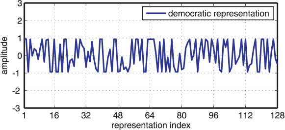
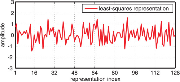
Figure 1: There are, in general, infinitely many ways to represent a signal as a linear combination of columns from an overcomplete matrix. In this example, we compare the representations of a given signal vector that are optimal according to three different criteria, i.e., minimum $\ell_{\infty}$, $\ell_{2}$, and $\ell_{1}$-norm, using an overcomplete $64\times 128$ subsampled DCT matrix; (a) democratic ($\ell_{\infty}$-norm) representation ($11.1$ dB PAPR); (b) least-squares ($\ell_{2}$-norm) representation ($16.2$ dB PAPR); (c) sparse ($\ell_{1}$-norm) representation ($29.9$ dB PAPR). We see that the democratic representation has (i) most of its entries’ magnitudes at the same maximum level and (ii) very small dynamic range (also in terms of the PAPR).

1.1 Application Examples

1.1.1 Vector quantization

Element-wise quantization of democratic representations affects all entries of $\dot{}\mathbf{x}$ equally, which renders them less susceptible to quantization noise compared with direct quantization of the signal vector $\mathbf{y}$ [1]. Moreover, the corruption of a few entries of $\dot{}\mathbf{x}$ results in only a small error and, therefore, computing $\mathbf{y}=\mathbf{D}\dot{}\mathbf{x}$ after, e.g., transmission over an unreliable communication channel [4] or storage in unreliable memory cells [5], enables one to obtain a robust estimate of the signal vector $\mathbf{y}$.

1.1.2 Peak-to-average power ratio (PAPR) reduction

Wireless communication systems employing orthogonal frequency division multiplexing (OFDM) typically require linear and power-inefficient radio-frequency (RF) components (e.g., power amplifiers) to avoid unwanted signal distortions or out-of-band radiation, as OFDM signals are prone to exhibit a large peak-to-average power ratio (PAPR) (also called the “crest factor”) [6]; see eq:pardefinition for the PAPR definition used in this paper. By allocating certain unused OFDM tones, which is known as tone reservation [7], or by exploiting the excess degrees-of-freedom in large-scale multi-antenna wireless systems (often called massive MIMO systems), one can transmit democratic representations, which significantly reduce the PAPR [8]. Hence, transmitting democratic representations, instead of conventional (unprocessed) OFDM signals, substantially alleviates the need for expensive and power-inefficient RF components. The example in fig:example confirms that the democratic representation exhibits substantially lower PAPR compared to a least-squares or sparse representation.

1.1.3 Approximate nearest neighbor search

Signal representations obtained from the problem $(\text{P}^{\,\varepsilon}_{\infty})$ also find use in the identification of approximate nearest neighbors in high-dimensional spaces [9]. The underlying idea is to compute a representation $\dot{}\mathbf{x}$ for the query vector $\mathbf{y}$. For certain matrices $\mathbf{D}$, the resulting representations are democratic and hence, resemble to an antipodal signal for which most coefficients take the values $-\alpha$ or $+\alpha$ for some $\alpha>0$; see the democratic representation example in fig:example where $\alpha\approx 1$. This property of the coefficients of $\dot{}\mathbf{x}$ can then be used to efficiently find approximate nearest vectors in an $N$-dimensional Hamming space.

1.1.4 Robotics and control

Kinematically redundant robots or manipulators admit infinitely many inverse solutions. Certain applications require a solution that minimizes the maximum force, acceleration, torque, or joint velocity, rather than minimizing the energy or power. Hence, in many practical situations, one is typically interested in solving problems of the form $(\text{P}^{\,\varepsilon}_{\infty})$ to obtain democratic representations with provably small $\ell_{\infty}$-norm, rather than minimum-energy (or least-squares) representations (the democratic representation in fig:example has significantly smaller $\ell_{\infty}$-norm compared to the other two representations); corresponding practical application examples have been discussed in [10, 11, 12].

1.1.5 Recovery conditions for sparse signal recovery

As shown in [13], the $\ell_{\infty}$-norm of the representation obtained by solving a specific instance of $(\text{P}^{\,\varepsilon}_{\infty})$ with $\varepsilon=0$ can be used to verify uniqueness and robustness conditions for $\ell_{1}$-norm-based (analysis and synthesis) sparse signal recovery problems. Such recovery conditions are of particular interest in the emerging fields of sparse signal recovery [14, 15, 16] and compressive sensing (CS) [17, 18, 19, 20].

1.2 What About Signal Recovery?

The problem $(\text{P}^{\,\varepsilon}_{\infty})$ with $\varepsilon=0$ can be used to recover antipodal (or binary-valued) signals, i.e., vectors with coefficients belonging to the set $\{-\alpha,+\alpha\}$ for $\alpha>0$ from the underdetermined system of linear equations $\mathbf{y}=\mathbf{D}\mathbf{x}$, provided that the matrix $\mathbf{D}$ meets certain conditions [21, 22, 23, 24]. The main focus here is, however, on (i) properties of democratic representations having minimal $\ell_{\infty}$-norm and small dynamic range, and (ii) their efficient computation, rather than on the recovery of a given antipodal vector $\mathbf{x}$ from the set of linear equations $\mathbf{y}=\mathbf{D}\mathbf{x}$ and corresponding uniqueness conditions. We refer the interested reader to [21, 22, 23, 24] for the details on antipodal signal recovery via $\ell_{\infty}$-norm minimization in noiseless and noisy settings.

1.3 Relevant Prior Art on $\ell_{\infty}$-Norm Minimization

Results for minimizing the maximum amplitude of continuos, real-valued signals subject to linear constraints reach back to the 1960s, when Neustadt [25] studied the so-called minimum-effort control problem. In 1971, Cadzow proposed a corresponding practicable algorithm suitable for low-dimensional systems, where he proposed to solve the following real-valued, convex $\ell_{\infty}$-norm minimization problem [10]:

$$(\text{P}_{\infty})\quad\underset{\tilde{}\mathbf{x}\in\mathbb{R}^{N}}{\text{minimize}}\,\,\mathopen{}\left\lVert\tilde{}\mathbf{x}\right\rVert_{\infty}\quad\text{subject to}\,\,\mathbf{y}=\mathbf{D}\tilde{}\mathbf{x}.$$

Note that this problem coincides to a real-valued version of $(\text{P}^{\,\varepsilon}_{\infty})$ with $\varepsilon=0$. Specifically, in [10] it was shown that, for a large class of matrices $\mathbf{D}$, there exists a solution $\dot{}\mathbf{x}$ to $(\text{P}_{\infty})$ for which a dominant portion of the entries’ magnitudes correspond to $\mathopen{}\left\lVert\dot{}\mathbf{x}\right\rVert_{\infty}$, whereas only a small fraction of the entries may have smaller magnitude; this result has been rediscovered recently by Fuchs in [2].

Another line of research that characterizes signal representations $\mathbf{x}$ with small (but not necessarily minimal) $\ell_{\infty}$-norm subject to $\mathbf{y}=\mathbf{D}\mathbf{x}$ have been established in 2010 by Lyubarskii and Vershynin [1]. In particular, [1] proves the existence of matrices $\mathbf{D}$ with arbitrarily small redundancy parameter $\lambda=N/M>1$ for which every signal vector $\mathbf{y}$ has a democratic representation $\mathbf{x}$ satisfying

$$\mathopen{}\left\lVert\mathbf{x}\right\rVert_{\infty}\leq\frac{K}{\sqrt{N}}\mathopen{}\left\lVert\mathbf{y}\right\rVert_{2}.$$ (1)

Here, $K$ is a (preferably small) constant that only depends on the redundancy parameter $\lambda$. The existence of such signal representations for certain sets of matrices can either be shown using fundamental results obtained by Kashin [26], Garnaev and Gluskin [27], or by analyzing the signal representations obtained via the iterative algorithm proposed in [1]. The latter (constructive) approach relies on an uncertainty principle (UP) for the matrix $\mathbf{D}$, which establishes a fundamental connection between the constant $K$ in eq:kashinrepdef and sensing matrices commonly used in sparse signal recovery and CS [17, 28].

1.4 Contributions

In this paper, we derive and investigate a host of fundamental properties for signal representations $\dot{}\mathbf{x}$ obtained from the $\ell_{\infty}$-norm minimization problem $(\text{P}^{\,\varepsilon}_{\infty})$. In particular, we analyze its Lagrange dual problem to derive a refined and more general version of the bound on the $\ell_{\infty}$-norm of the signal representation $\dot{}\mathbf{x}$ established in [1]. We characterize magnitude properties of the signal representations $\dot{}\mathbf{x}$ obtained by solving $(\text{P}^{\,\varepsilon}_{\infty})$, and we develop bounds on the resulting PAPR, which is of particular interest in OFDM-based communication systems. As a byproduct of our analysis, we present the Lagrange duals to a variety of optimization problems, such as $\ell_{1}$-norm minimization, which is often used for sparse signal recovery and compressive sensing. We then discuss classes of matrices that enable the computation of democratic representations via $(\text{P}^{\,\varepsilon}_{\infty})$. Furthermore, we develop two computationally efficient algorithms to solve $(\text{P}^{\,\varepsilon}_{\infty})$, referred to as CRAM (short for convex reduction of amplitudes) and CRAMP (short for CRAM for Parseval frames). CRAM is suitable for arbitrary matrices $\mathbf{D}$ and approximation parameters $\varepsilon\in[0,\infty)$, whereas CRAMP exhibits lower complexity than CRAM for $\varepsilon=0$ and Parseval frames. We provide numerical experiments to support our analysis and conclude by demonstrating the efficacy of democratic representations for PAPR reduction in a DVB-T2-based broadcast system [29].

1.5 Notation

Lowercase boldface letters stand for column vectors and uppercase boldface letters designate matrices. For a matrix $\mathbf{A}$, we denote its conjugate transpose and spectral norm by $\mathbf{A}^{H}$ and $\mathopen{}\left\lVert\mathbf{A}\right\rVert_{2,2}=\sqrt{\lambda_{\text{max}}(\mathbf{A}^{H}\mathbf{A})}$, respectively, where $\lambda_{\text{max}}(\mathbf{A}^{H}\mathbf{A})$ denotes the maximum eigenvalue of $\mathbf{A}^{H}\mathbf{A}$. We use $\mathbf{0}_{M\times N}$ and $\mathbf{1}_{M\times N}$ to denote the all-zeros and all-ones matrix of dimension $M\times N$, respectively. The $k^{\text{th}}$ entry of a vector $\mathbf{a}$ is designated by $[\mathbf{a}]_{k}$, and $\Re\{\mathbf{a}\}$ and $\Im\{\mathbf{a}\}$ represent its real and imaginary part, respectively. We define the $\ell_{p}$-norm of the vector $\mathbf{a}\in\mathbb{C}^{N}$ as follows:

$$\|{\mathbf{a}}\|_{p}=\left\{\begin{array}[]{ll}\left(\sum_{k=1}^{N}\mathopen{}\left\lvert[\mathbf{a}]_{k}\right\rvert^{p}\right)^{\!1/p}&\text{if}\,\,\,1\leq p<\infty\\[5.69046pt] \max_{k\in\{1,\ldots,N\}}\mathopen{}\left\lvert[\mathbf{a}]_{k}\right\rvert&\text{if}\,\,\,p=\infty.\end{array}\right.$$

We also make use of the (non-standard) $\ell_{\widetilde{\infty}}$-norm [30] defined as $\mathopen{}\left\lVert\mathbf{a}\right\rVert_{\widetilde{\infty}}=\max\!\big{\{}\mathopen{}\left\lVert\Re\{\mathbf{a}\}\right\rVert_{\infty}\!,\mathopen{}\left\lVert\Im\{\mathbf{a}\}\right\rVert_{\infty}\!\big{\}}$. The notation $\dot{}\mathbf{x}$ is used to refer to the solutions to the problem $(\text{P}^{\,\varepsilon}_{\infty})$. Sets are designated by uppercase Greek letters; the cardinality of the set $\Omega$ is $\mathopen{}\left\lvert\Omega\right\rvert$. The notation $\textrm{supp}(\mathbf{a})$ designates to the support set of the vector $\mathbf{a}$, i.e., the set of indices associated to non-zero entries in $\mathbf{a}$. The sign (or phase) of a complex-valued scalar $x\in\mathbb{C}$ is defined as

$$\operatorname{sign}(x)=\left\{\begin{array}[]{ll}x/\mathopen{}\left\lvert x\right\rvert&\text{if}\,\,\,x\neq 0\\[4.26773pt] 0&\text{if}\,\,\,x=0.\end{array}\right.$$

We use $\operatorname{sign}(\mathbf{a})$ and $\mathrm{abs}(\mathbf{a})$ to denote the entry-wise application of the sign function and absolute value to the vector $\mathbf{a}$, respectively.

1.6 Organization of the Paper

The remainder of the paper is organized as follows. Section 2 introduces the essentials of frames and the uncertainty property (UP). In sec:theory, we develop the concept of democratic representations. Our main results are detailed in sec:properties. sec:UPsatisfyingmatrices reviews suitable classes of matrices that satisfy the UP and enable the computation of democratic representations. sec:algorithmyipee develops computationally efficient algorithms for solving $(\text{P}^{\,\varepsilon}_{\infty})$. sec:simulation provides numerical experiments and showcases the efficacy of democratic representations for PAPR reduction. We conclude in sec:conclusions. Most proofs are relegated to the Appendices.

2 Frames and the Uncertainty Principle

2.1 Frames

We often require the over-complete matrix $\mathbf{D}\in\mathbb{C}^{M\times N}$ with $M<N$ to satisfy the following property.

Definition 1 (Frame [31])

A matrix $\mathbf{D}\in\mathbb{C}^{M\times N}$ with $M\leq N$ is called a frame if

$$A\mathopen{}\left\lVert\mathbf{w}\right\rVert_{2}^{2}\leq\mathopen{}\left\lVert\mathbf{D}^{H}\mathbf{w}\right\rVert_{2}^{2}\leq B\mathopen{}\left\lVert\mathbf{w}\right\rVert_{2}^{2}$$

holds for any vector $\mathbf{w}\in\mathbb{C}^{M}$ with $A\in\mathbb{R}$, $B\in\mathbb{R}$, and $0<A\leq B<\infty$.

The tightest possible constants $A$ and $B$ are called the lower and upper frame bounds, respectively. The frame $\mathbf{D}$ is called a tight frame if $A=B$. Furthermore, if $A=B=1$, then $\mathbf{D}$ is a Parseval frame [31]. In what follows, we exclusively study the finite-dimensional setting (i.e., where $M,N<\infty$) and thus $B<\infty$. Further, because our frame definition requires $A$ to be strictly positive, $\mathbf{D}$ is guaranteed to be full rank. Thus, $(\text{P}^{\,\varepsilon}_{\infty})$ is feasible for any frame $\mathbf{D}$ and $\varepsilon\geq 0$.

2.2 Full-Spark Frames

The next definition is concerned with the spark of a frame, which represents the cardinality of the smallest subset of linearly dependent frame columns.

Definition 2 (Full-spark frame [32])

A frame $\mathbf{D}\in\mathbb{C}^{M\times N}$ is called a full-spark frame if the columns of every $M\times M$ sub-matrix of $\mathbf{D}$ are linearly independent.

Full-spark frames have spark $M+1$ and are ubiquitous in sparse signal recovery and CS (see [32] for a review). Even though verifying the full-spark property of an arbitrary matrix is, in general, a hard problem [33], many frames are known to be full spark. For example, any subset of rows from a Fourier matrix of prime dimension forms a full-spark frame [32, 34]. Further, Vandermonde matrices with $M\leq N$ having distinct basis entries are known to be full spark frames [35, 32]. In addition, randomized constructions also exist that generate full-spark frames with high probability. In particular, if the entries of an $M\times N$ matrix with $M<N$ are generated from independent continuous random variables, then the resulting matrix is a full-spark frame with probability one (see [36] for a formal proof).

2.3 The Uncertainty Principle (UP)

Several of the results derived in this paper rely upon the uncertainty principle (UP) introduced in [1].

Definition 3 (Uncertainty principle [1])

We say that the frame $\mathbf{D}\in\mathbb{C}^{M\times N}$ satisfies the UP with parameters $\eta\in\mathbb{R}^{+}$ and $\delta\in(0,1)$ if

$$\mathopen{}\left\lVert\mathbf{D}\mathbf{x}\right\rVert_{2}\leq\eta\mathopen{}\left\lVert\mathbf{x}\right\rVert_{2}$$ (2)

holds for all (sparse) vectors $\mathbf{x}\in\mathbb{C}^{N}$ satisfying $\mathopen{}\left\lvert\textrm{supp}(\mathbf{x})\right\rvert\leq\delta N$.

We emphasize that (2) is trivially satisfied for $\eta=\mathopen{}\left\lVert\mathbf{D}\right\rVert_{2,2}$ and for arbitrary vectors with $\mathopen{}\left\lvert\textrm{supp}(\mathbf{x})\right\rvert\leq N$. However, as in [1], we are particularly interested in frames satisfying the UP with parameters $\eta<\mathopen{}\left\lVert\mathbf{D}\right\rVert_{2,2}$ and $\delta<1$. For simplicity, we say that frames satisfying definition (3) with such non-trivial parameters “satisfy the UP.”

Verifying the UP with parameters $\eta<\mathopen{}\left\lVert\mathbf{D}\right\rVert_{2,2}$ and $\delta<1$ for a given frame $\mathbf{D}$ requires, in general, a combinatorial search over all $\delta N$-sparse vectors [33]. Nevertheless, many classes of frames are known to satisfy the UP with high probability (see [1] and sec:UPsatisfyingmatrices for more details). We finally note that frames satisfying the UP are strongly related to sensing matrices with small restricted isometry constants; such matrices play a central role in CS [17, 28, 20].

3 Democratic Representations

We next introduce the concept of democratic representations and define the democracy constants.

3.1 Democratic Representations

For $M<N$ and $\varepsilon<\mathopen{}\left\lVert\mathbf{y}\right\rVert_{2}$, there exist, in general, an infinite number of representations $\mathbf{x}$ for a given signal vector $\mathbf{y}$ that satisfy $\mathopen{}\left\lVert\mathbf{y}-\mathbf{D}\mathbf{x}\right\rVert_{2}\leq\varepsilon$. In the remainder of the paper, we are particularly interested in representations for which every entry $x_{i}$, $i=1,\ldots,N$ is of approximately the same importance. In particular, we seek so-called democratic representations, which have provably small $\ell_{\infty}$-norm and for which all magnitudes are approximately equal. In order to make the concept of democratic representations more formal, we use the following definition.

Definition 4 (Democracy constants)

Let $\mathbf{D}\in\mathbb{C}^{M\times N}$ be a given frame. Assume we obtain a signal representation $\dot{}\mathbf{x}$ for every vector $\mathbf{y}\in\mathbb{C}^{M}$ by solving $(\text{P}^{\,\varepsilon}_{\infty})$ with $\varepsilon\leq\mathopen{}\left\lVert\mathbf{y}\right\rVert_{2}$. We define the lower and upper democracy constants $K_{\text{l}}\in\mathbb{R}$ and $K_{\text{u}}\in\mathbb{R}$ to be the largest and smallest constants for which

$$\frac{K_{\text{l}}}{\sqrt{N}}\big{(}\mathopen{}\left\lVert\mathbf{y}\right\rVert_{2}-\varepsilon\big{)}\leq\mathopen{}\left\lVert\dot{}\mathbf{x}\right\rVert_{\infty}\leq\frac{K_{\text{u}}}{\sqrt{N}}\big{(}\mathopen{}\left\lVert\mathbf{y}\right\rVert_{2}-\varepsilon\big{)}$$ (3)

holds for every pair $\dot{}\mathbf{x}$ and $\mathbf{y}$, and for any $0\leq\varepsilon\leq\mathopen{}\left\lVert\mathbf{y}\right\rVert_{2}$.

We note that the democracy constants $K_{\text{l}}$ and $K_{\text{u}}$ depend only on properties of the frame $\mathbf{D}$ and the fact that all signal representations $\dot{}\mathbf{x}$ are obtained via $(\text{P}^{\,\varepsilon}_{\infty})$, and not on the signal vector $\mathbf{y}$. Note that def:democracyconstants enables us to analyze a generalized and refined setting of the special case eq:kashinrepdef studied in [1] (see our results in sec:properties).

In what follows, we are interested in (i) classes of frames for which the lower and upper democracy constants $K_{\text{l}}$, $K_{\text{u}}$ are both close to $1$, and (ii) computationally efficient algorithms that provably deliver such signal representations. In particular, if $K_{\text{l}}\approx 1\approx K_{\text{u}}$, then all signal representations $\dot{}\mathbf{x}$ have similar $\ell_{\infty}$-norm and every entry will have a maximum magnitude of $1/\sqrt{N}$ (assuming $\varepsilon=0$ and $\mathopen{}\left\lVert\mathbf{y}\right\rVert_{2}=1$). Since this property evenly spreads the signal vector’s energy $\mathopen{}\left\lVert\mathbf{y}\right\rVert_{2}$ across all entries of $\dot{}\mathbf{x}$, we call such representations democratic.

Definition 5 (Democratic representations)

Let $\mathbf{D}\in\mathbb{C}^{M\times N}$ be a given frame. If the associated democracy constants $K_{\text{l}}$ and $K_{\text{u}}$ are both close to $1$, then the signal representations $\dot{}\mathbf{x}$ obtained by $(\text{P}^{\,\varepsilon}_{\infty})$ are called democratic representations.

3.2 Computing Democratic Representations

In order to compute representations $\mathbf{x}$ having small (but not necessarily minimal) $\ell_{\infty}$-norm subject to the set of linear equations $\mathbf{y}=\mathbf{D}\mathbf{x}$, one can use the iterative algorithm proposed in [1]. This method efficiently computes such representations for real-valued and approximate Parseval frames, i.e., frames $\mathbf{D}\in\mathbb{R}^{M\times N}$ satisfying the UP in [1] with Frame bounds $A=1-\xi$ and $B=1+\xi$ for some small $\xi\geq 0$. However, the algorithm in [1] (i) does not solve $(\text{P}^{\,\varepsilon}_{\infty})$ and is, in general, not guaranteed to find representations $\dot{}\mathbf{x}$ having the smallest $\ell_{\infty}$-norm, (ii) requires knowledge of the UP parameters $\eta$, $\delta$, (iii) was introduced for real-valued systems, and (iv) is only guaranteed to converge for approximate Parseval frames. Moreover, if one is interested in approximate representations $\mathbf{x}$ for which $\mathopen{}\left\lVert\mathbf{y}-\mathbf{D}\mathbf{x}\right\rVert_{2}>0$ rather than in perfect representations satisfying $\mathbf{y}=\mathbf{D}\mathbf{x}$, the algorithm in [1] must be modified accordingly. In order to overcome the limitations of the algorithm in [1], we propose to directly solve the convex problem $(\text{P}^{\,\varepsilon}_{\infty})$ instead; sec:algorithmyipee will detail two corresponding (and computationally efficient) algorithms.

4 Main Results

We now analyze several key properties of signal representations $\dot{}\mathbf{x}$ obtained from solving $(\text{P}^{\,\varepsilon}_{\infty})$. sec:extremevalues studies magnitude properties of the solutions to $(\text{P}^{\,\varepsilon}_{\infty})$. sec:lagrangedual introduces the Lagrange dual problem to $(\text{P}^{\,\varepsilon}_{\infty})$, which is key in the proofs of Sections 4.3 and 4.4, where we develop bounds on the lower and upper democracy constants $K_{\text{l}}$ and $K_{\text{u}}$, respectively. sec:PAR analyzes the PAPR characteristics of democratic representations, and sec:devotedtodominikseethaler outlines an extension of our results to the $\ell_{\widetilde{\infty}}$-norm.

4.1 Extreme Values of Solutions to $(\text{P}^{\,\varepsilon}_{\infty})$

The magnitudes of signal representations obtained via $(\text{P}^{\,\varepsilon}_{\infty})$ exhibit specific and practically relevant properties. To study them, we need the following definition.

Definition 6 (Extreme and moderate entries)

Given a vector $\mathbf{x}\in\mathbb{C}^{N}$, we call an entry $x_{i}$ extreme if $|x_{i}|=\|\mathbf{x}\|_{\infty}$; we further call an entry $x_{i}$ moderate if $|x_{i}|<\|\mathbf{x}\|_{\infty}$.

Without any specific assumptions on the overcomplete matrix $\mathbf{D}$ (apart from being full-rank), we next show that there always exists a solution to $(\text{P}^{\,\varepsilon}_{\infty})$ with a large portion of extreme entries (see app:demsExist for the proof). In words, a democratic representation is one with a large portion of extreme entries.

Lemma 1 (Democratic representations exist)

For any full-rank matrix $\mathbf{D}\in\mathbb{C}^{M\times N}$ with $M\leq N$, the problem $(\text{P}^{\,\varepsilon}_{\infty})$ admits a solution $\dot{}\mathbf{x}$ with at least $N-M+1$ extreme entries.

This result implies that there exist signal representations $\dot{}\mathbf{x}$ for which a large number of (extreme) entries have equal magnitude. In particular, by increasing the redundancy $\lambda=N/M$ of $\mathbf{D}$, the problem $(\text{P}^{\,\varepsilon}_{\infty})$ admits representations for which the number of extreme values is arbitrarily close to $N$.

The next result shows that—given the matrix $\mathbf{D}$ is a full-spark frame—every solution to the problem $(\text{P}^{\,\varepsilon}_{\infty})$ has a bounded minimal number of extreme entries (see app:alwaysDem for the proof).

Lemma 2 (All representations are democratic)

If the frame $\mathbf{D}$ has full spark, then every solution to $(\text{P}^{\,\varepsilon}_{\infty})$ has at least $N-M+1$ extreme entries.

This result implies that for full-spark frames with large redundancy $\lambda=M/N$, every solution to $(\text{P}^{\,\varepsilon}_{\infty})$ is a democratic representation (with most entries being extreme). As noted in sec:fullsparkframes, a large number of deterministic and random constructions of full-spark frames are known. Hence, solving $(\text{P}^{\,\varepsilon}_{\infty})$ allows the computation of democratic representations for a large number of frames. In addition, lem:alwaysDem enables us to obtain the following $\ell_{\infty}$/$\ell_{2}$-norm inequality.

Theorem 3 (Democratic $\ell_{\infty}$/$\ell_{2}$-norm inequality)

If $\mathbf{D}$ is a full-spark frame, then

$$\sqrt{N-M+1}\mathopen{}\left\lVert\dot{}\mathbf{x}\right\rVert_{\infty}\leq\mathopen{}\left\lVert\dot{}\mathbf{x}\right\rVert_{2}$$ (4)

holds for every representation $\dot{}\mathbf{x}$ obtained by solving $(\text{P}^{\,\varepsilon}_{\infty})$.

Proof 1

The proof immediately follows from lem:alwaysDem and the straightforward inequality $\mathopen{}\left\lVert\dot{}\mathbf{x}\right\rVert_{2}^{2}=\sum_{i=1}^{N}|\dot{x}_{i}|^{2}\geq(N-M+1)\mathopen{}\left\lVert\dot{}\mathbf{x}\right\rVert_{\infty}^{2}$.

We note that the norm inequality (4) is stronger than the standard norm bound $\mathopen{}\left\lVert\mathbf{x}\right\rVert_{\infty}\leq\mathopen{}\left\lVert\mathbf{x}\right\rVert_{2}$ for $M<N$ (which holds for arbitrary vectors $\mathbf{x}$). More importantly, as we show below in sec:PAR, the refined norm inequality (4) is particularly useful for characterizing the limits of PAPR reduction methods that rely on democratic representations.

We conclude by noting that results related to Lemmata 1 and 2 for the special problem $(\text{P}^{\,\varepsilon}_{\infty})$ with $\varepsilon=0$ have been developed in the literature [2, 10]. In particular, [10] establishes bounds on the minimum number of entries that satisfy $x_{i}\leq\mathopen{}\left\lVert\mathbf{x}\right\rVert_{\infty}$ (i.e., entries that are not necessarily extremal). This result, however, does not allow us to extract bounds on the number of extremal values, which is in contrast to Lemmata 1 and 2. Reference [2] mentions that signal representations obtained from $(\text{P}_{\infty})$ have, in general, exactly $N-M+1$ extreme entries. This result, however, is stated without proof and, more importantly, without explicitly specifying conditions on the classes of the matrices for which it is supposed to hold.

4.2 Lagrange Dual Problem

In order to derive bounds on the lower and upper democracy constants $K_{\text{l}}$ and $K_{\text{u}}$, respectively, and to study the PAPR behavior of solutions to $(\text{P}^{\,\varepsilon}_{\infty})$, we make use of the following theorem (see app:primaldualproblems for the proof).

Theorem 4 (Lagrange dual problem)

Let the $\ell_{p}$-norm primal problem (with $1\leq p\leq\infty$) be

$$(\text{P}^{\,\varepsilon}_{p})\quad\underset{\tilde{}\mathbf{x}\in\mathbb{C}^{N}}{\text{minimize}}\,\,\|{\tilde{}\mathbf{x}}\|_{p}\quad\text{subject to}\,\,\mathopen{}\left\lVert\mathbf{y}-\mathbf{D}\tilde{}\mathbf{x}\right\rVert_{2}\leq\varepsilon.$$

Then, the corresponding Lagrange dual problem is given by

$$(\text{D}^{\,\varepsilon}_{p})\quad\left\{\begin{array}[]{ll}\underset{\tilde{}\mathbf{z}\in\mathbb{C}^{M}}{\text{maximize}}&\Re\!\left(\mathbf{y}^{H}\tilde{}\mathbf{z}\right)-\varepsilon\mathopen{}\left\lVert\tilde{}\mathbf{z}\right\rVert_{2}\\[5.69046pt] \text{subject to}&\|\mathbf{D}^{H}\tilde{}\mathbf{z}\|_{d}\leq 1\end{array}\right.$$

with $1/p+1/d=1$; for $p=1$ we have $q=\infty$ and vice versa. The norm $\|\cdot\|_{d}$ corresponds to the dual norm of $\|\cdot\|_{p}$.

Note that thm:primaldualproblems includes not only the Lagrange dual to the problem $(\text{P}^{\,\varepsilon}_{\infty})$, but also other frequently studied optimization problems, such as the Lagrangian dual to $(\text{P}^{\,\varepsilon}_{1})$, which is often used for sparse signal recovery or CS.

4.3 Bound on Lower Democracy Constant $K_{\text{l}}$

In order to characterize the lower democracy constant $K_{l}$ for a given frame $\mathbf{D}$, we next derive a corresponding lower bound.

Lemma 5 (Lower democracy bound)

Let $\mathbf{D}\in\mathbb{C}^{M\times N}$ be a frame with upper frame bound $B$. Then, every vector $\mathbf{y}\in\mathbb{C}^{M}$ admits a signal representation $\dot{}\mathbf{x}$ with the following lower bound $\widetilde{K}_{\text{l}}$ on the lower democracy constant $K_{l}$ (see app:lowerkashinbound for the proof):

$$\widetilde{K}_{\text{l}}=\frac{1}{\sqrt{B}}\leq K_{\text{l}}.$$ (5)

The representations $\dot{}\mathbf{x}$ obtained from the problem $(\text{P}^{\,\varepsilon}_{\infty})$ are guaranteed to satisfy eq:lowerkashinbound, as the proof of lem:lowerkashinbound exploits properties of its solution. In the special case $\varepsilon=0$ and for Parseval frames, lem:lowerkashinbound guarantees that all vectors $\mathbf{y}$ admit a signal representation satisfying

$$\frac{\mathopen{}\left\lVert\mathbf{y}\right\rVert_{2}}{\sqrt{N}}\leq\mathopen{}\left\lVert\dot{}\mathbf{x}\right\rVert_{\infty}.$$

This lower bound was established previously in [1, Obs. 2.1b]. lem:lowerkashinbound generalizes this result to arbitrary frames and to representations for which $\varepsilon>0$. It is furthermore interesting to observe that the lower democracy bound in eq:lowerkashinbound only depends on the upper frame constant $B$ (and implicitly on the fact that frames satisfy $A>0$); this is in contrast to the bound on the upper democracy constant $K_{\text{u}}$ derived next.

4.4 Bound on Upper Democracy Constant $K_{\text{u}}$

In order to characterize the upper democracy constant $K_{u}$, we next derive an upper bound $\widetilde{K}_{\text{u}}$ on $K_{\text{u}}$ by using the uncertainty principle (UP) for frames (see app:proof_mainresult for the proof).

Theorem 6 (Upper democracy bound)

Let $\mathbf{D}\in\mathbb{C}^{M\times N}$ be a frame with frame bounds $A$, $B$ that satisfies the uncertainty principle (UP) with parameters $\eta$, $\delta$. Then, every signal vector $\mathbf{y}$ admits a signal representation $\dot{}\mathbf{x}$ with the following upper bound on the upper democracy constant:

$${K}_{\text{u}}\leq\widetilde{K}_{\text{u}}=\frac{\eta}{(A-\eta\sqrt{B})\sqrt{\delta}},$$ (6)

provided $A>\eta\sqrt{B}$.

The representations $\dot{}\mathbf{x}$ obtained from the problem $(\text{P}^{\,\varepsilon}_{\infty})$ are guaranteed to satisfy eq:maincondition, as the proof exploits properties of its solution. In addition, thm:main_result shows that if a frame $\mathbf{D}$ satisfies (i) $A>\eta\sqrt{B}$ and (ii) $\delta>0$, then one can compute democratic representations for every signal vector $\mathbf{y}$ by solving $(\text{P}^{\,\varepsilon}_{\infty})$. In addition, the condition $A>\eta\sqrt{B}$ indicates that the use of Parseval frames is beneficial in practice, i.e., leads to democratic representations with smaller $\ell_{\infty}$-norm—an observation that was made empirically by Fuchs [37]; corresponding simulation results are provided in sec:simulation. In order to achieve representations having provably small $\ell_{\infty}$-norm (close to $1$), one is typically interested in finding frames satisfying the UP with small $\eta$ and large $\delta$. Both properties can be achieved simultaneously for certain classes of frames (see [1] and sec:UPsatisfyingmatrices for corresponding examples).

We note that thm:main_result improves upon the results in [1]. In particular, the bound $\widetilde{K}_{\text{u}}$ in eq:maincondition is strictly smaller than the bound obtained in [1, Thms. 3.5 and 3.9]. To see this, consider the case of $\mathbf{D}$ being a Parseval frame and $\varepsilon=0$; this enables us to establish the following relation between the upper democracy bound $\widetilde{K}_{\text{u}}$ in eq:maincondition and the bound $K$ from [1, Thm. 3.5]:

$$\widetilde{K}_{\text{u}}=\frac{\eta}{(1-\eta)\sqrt{\delta}}<\frac{1}{(1-\eta)\sqrt{\delta}}=K.$$

The strict inequality follows from the fact that $\eta$ is required to be smaller than one, which is a consequence of $A>\eta\sqrt{B}$. Hence, by solving $(\text{P}^{\,\varepsilon}_{\infty})$ rather than using the algorithm proposed in [1], we arrive at an upper bound that is more tight (i.e., by a factor of $\eta$). For approximate Parseval frames satisfying $A=1-\xi$ and $B=1+\xi$ with $0\leq\xi<1$, the upper democracy bound in eq:maincondition continues to be superior to that in [1, Thm. 3.9]. Furthermore, thm:main_result also encompasses approximate representations ($\varepsilon>0$) and the case of complex-valued vectors and frames, which is in contrast to the results developed in [1].

4.5 PAPR Properties of Democratic Representations

4.5.1 PAPR reduction via democratic representations

Democratic representations can be used to (often substantially) reduce a signal’s dynamic range, which is typically characterized in terms of its PAPR (or “crest factor”) defined below. For example, the transmission of information-bearing signals over frequency-selective channels typically requires sophisticated equalization schemes at the receive side. Orthogonal frequency-division multiplexing (OFDM) [6] is a well-established way of reducing the computational complexity of equalization (compared to conventional equalization schemes). Unfortunately, OFDM signals are known to suffer from a high PAPR, which requires linear RF components (e.g., power amplifiers). Since linear RF components are, in general, more costly and less power efficient compared to their non-linear counterparts, practical transceiver implementations often deploy sophisticated PAPR-reduction schemes [38]. Prominent approaches for reducing the PAPR exploit either certain reserved OFDM tones [7] or the excess degrees-of-freedom in large-scale multi-antenna wireless systems [8]. As we will show next, democratic representations computed via $(\text{P}^{\,\varepsilon}_{\infty})$ have intrinsically low PAPR.

We start by defining the PAPR of arbitrary vectors $\mathbf{x}$.

Definition 7 (Peak-to-average power ratio)

Let $\mathbf{x}\in\mathbb{C}^{N}$ be a nonzero vector. Then, the peak-to-average power ratio (PAPR) (or “crest factor”) of $\mathbf{x}$ is defined as

$$\textit{PAPR}(\mathbf{x})=\frac{N\mathopen{}\left\lVert\mathbf{x}\right\rVert_{\infty}^{2}}{\mathopen{}\left\lVert\mathbf{x}\right\rVert_{2}^{2}}.$$ (7)

Note that for arbitrary vectors $\mathbf{x}\in\mathbb{C}^{N}$, the PAPR satisfies the following inequalities:

$$1\leq\textit{PAPR}(\mathbf{x})\leq N,$$ (8)

an immediate consequence of standard norm bounds. The lower bound (best case) is achieved for signals having constant amplitude (or modulus), whereas the upper bound (worst case) is achieved by vectors having a single nonzero entry. As we will show next, the worst-case PAPR of signal representations obtained through $(\text{P}^{\varepsilon}_{\infty})$ is typically much smaller than the upper bound in eq:simpleparbound suggests. To show this, we next bound the PAPR of signal representations obtained through $(\text{P}^{\varepsilon}_{\infty})$ with the aid of (i) the democratic $\ell_{\infty}$/$\ell_{2}$-norm inequality in eq:fancypantsnormbound or (ii) the upper democracy bound in eq:maincondition.

The following PAPR bound only depends on the dimensions of the full-spark frame $\mathbf{D}$.

Theorem 7 (Full-spark PAPR bound)

Let $\mathbf{D}\in\mathbb{C}^{M\times N}$ be a full-spark frame. Then, the PAPR of every signal representation $\dot{}\mathbf{x}$ obtained by solving $(\text{P}^{\,\varepsilon}_{\infty})$ satisfies

$$\textit{PAPR}(\dot{}\mathbf{x})\leq\frac{N}{N-M+1}$$ (9)

for vectors $\mathbf{y}\in\mathbb{C}^{M}$ satisfying $\mathopen{}\left\lVert\mathbf{y}\right\rVert_{2}\neq 0$ and $\varepsilon<\mathopen{}\left\lVert\mathbf{y}\right\rVert_{2}$.

Proof 2

The proof directly follows from lem:alwaysDem and the PAPR definition eq:pardefinition by replacing $\mathopen{}\left\lVert\dot{}\mathbf{x}\right\rVert_{2}^{2}$ by $(N-M+1)\mathopen{}\left\lVert\dot{}\mathbf{x}\right\rVert_{\infty}^{2}$.

thm:parbound1 implies that $\ell_{\infty}$-norm minimization can be used as a practical and efficient substitute for minimizing the PAPR in (7) directly, which is difficult to achieve in practice. In addition, we observe that frames with large redundancy parameter $\lambda=N/M$ enable the computation of representations with arbitrary low PAPR (by increasing the dimension $N$). To see this, let $\lambda\to\infty$, which results in the following asymptotic bound:

$$\textit{PAPR}(\dot{}\mathbf{x})\leq({1+1/N})^{-1}.$$

The following theorem provides a PAPR bound for frames that satisfy the UP with parameters $\eta$, $\delta$ (see app:parbound for the proof).

Theorem 8 (UP-based PAPR bound)

Let $\mathbf{D}\in\mathbb{C}^{M\times N}$ be a frame with the upper democracy bound $\widetilde{K}_{u}$ in eq:maincondition. Then, the PAPR of every signal representation $\dot{}\mathbf{x}$ obtained via $(\text{P}^{\,\varepsilon}_{\infty})$ satisfies the following bound:

$$\textit{PAPR}(\dot{}\mathbf{x})\leq\widetilde{K}_{\text{u}}^{2}B$$ (10)

for vectors $\mathbf{y}\in\mathbb{C}^{M}$ with $\mathopen{}\left\lVert\mathbf{y}\right\rVert_{2}\neq 0$ and $\varepsilon<\mathopen{}\left\lVert\mathbf{y}\right\rVert_{2}$.

thm:parbound reveals that frames satisfying the UP and having a small upper democracy bound $\widetilde{K}_{\text{u}}$ are particularly effective in terms of reducing the PAPR. A practically relevant example of frames satisfying these properties are randomly subsampled discrete Fourier transform (DFT) matrices, which naturally appear in OFDM-based tone-reservation schemes for PAPR reduction (see, e.g., [7] for the details). A corresponding application example is shown below in sec:applicationexample.

It is worth mentioning that the PAPR bounds (9) and (10) do not depend on the approximation parameter $\varepsilon$. Hence, in practice, an increase in $\varepsilon$ (as long as $\varepsilon<\mathopen{}\left\lVert\mathbf{y}\right\rVert_{2}$) is expected to not affect the PAPR of the democratic representation $\dot{}\mathbf{x}$, which is in contrast to (3).

4.5.2 Transmit power increase

If democratic representations are used for PAPR reduction, e.g., in an OFDM-based communication system, then it is important to realize that transmitting $\dot{}\mathbf{x}$ instead of the minimum-power (or least squares) solution $\hat{}\mathbf{x}$ obtained from

$$(\text{P}^{\,\varepsilon}_{2})\quad\underset{\tilde{}\mathbf{x}}{\text{minimize}}\,\,\mathopen{}\left\lVert\tilde{}\mathbf{x}\right\rVert_{2}\quad\text{subject to}\,\,\mathopen{}\left\lVert\mathbf{y}-\mathbf{D}\tilde{}\mathbf{x}\right\rVert_{2}\leq\varepsilon,$$

may result in a larger transmit power. Therefore, it is of practical interest to study the associated power increase (PI), defined as

$$\textit{PI}=\frac{\mathopen{}\left\lVert\dot{}\mathbf{x}\right\rVert_{2}^{2}}{\mathopen{}\left\lVert\hat{}\mathbf{x}\right\rVert_{2}^{2}},$$ (11)

when transmitting democratic representations $\dot{}\mathbf{x}$ instead of the least-squares representation $\hat{}\mathbf{x}$ of $(\text{P}^{\,\varepsilon}_{2})$. The following result provides an upper bound on the PI (see app:gainbound for the proof).

Theorem 9 (Power increase)

Let $\mathbf{D}\in\mathbb{C}^{M\times N}$ be a frame with the upper frame bound $B$ and upper democracy constant $K_{u}$. Then, the power increase, PI, in eq:powerincreasedef of every signal representation $\dot{}\mathbf{x}$ obtained by solving $(\text{P}^{\,\varepsilon}_{\infty})$ satisfies

$$1\leq\textit{PI}\leq\widetilde{K}_{\text{u}}^{2}B$$ (12)

for vectors $\mathbf{y}\in\mathbb{C}^{M}$ satisfying $\mathopen{}\left\lVert\mathbf{y}\right\rVert_{2}\neq 0$ and $\varepsilon<\mathopen{}\left\lVert\mathbf{y}\right\rVert_{2}$.

It is interesting to observe that the RHS of the bound eq:powerincrease in thm:gainbound coincides with the RHS of the PAPR bound eq:parbound. As a consequence, the use of frames that yield good PAPR reduction properties also guarantee a small power increase compared to directly transmitting a least-squares representation.

4.6 The $\ell_{\widetilde{\infty}}$-Norm and Its Implications

In certain applications, one might be interested in minimizing the $\ell_{\widetilde{\infty}}$-norm rather than the $\ell_{\infty}$-norm of the signal representation. Such representations can be useful if the PAPR of both the real and imaginary parts need to be minimized individually (see, e.g., [8]). In order to derive properties of signal representations obtained by solving

$$(\text{P}^{\,\varepsilon}_{\widetilde{\infty}})\quad\underset{\tilde{}\mathbf{x}\in\mathbb{C}^{N}}{\text{minimize}}\,\,\mathopen{}\left\lVert\tilde{}\mathbf{x}\right\rVert_{\widetilde{\infty}}\quad\text{subject to}\,\,\mathopen{}\left\lVert\mathbf{y}-\mathbf{D}\tilde{}\mathbf{x}\right\rVert_{2}\leq\varepsilon,$$

we can use the following inequalities developed in [30, Eq. 78]:

$$\frac{1}{\sqrt{2}}\mathopen{}\left\lVert\mathbf{x}\right\rVert_{\infty}\leq\mathopen{}\left\lVert\mathbf{x}\right\rVert_{\widetilde{\infty}}\leq\mathopen{}\left\lVert\mathbf{x}\right\rVert_{\infty}.$$ (13)

These inequalities imply that all properties derived from the original problem $(\text{P}^{\,\varepsilon}_{\infty})$ hold as well for democratic representations obtained by $(\text{P}^{\,\varepsilon}_{\widetilde{\infty}})$ up to a factor of at most two.

5 Frames that Enable Democratic Representations

As shown in [1], random orthogonal matrices, random partial DFT matrices, and random sub-Gaussian matrices satisfy the UP in def:upforframes with high probability. Hence, matrices drawn from such classes are particularly suitable for the computation of democratic representations with small $\ell_{\infty}$-norm and for applications requiring low PAPR. As an example, we briefly restate a result obtained in [1] for matrices whose entries are chosen i.i.d.  sub-Gaussian.

Definition 8 (Sub-Gaussian RV [1, Def. 4.5])

A random variable $X$ is called sub-Gaussian with parameter $\beta$ if

$$\Pr\{\mathopen{}\left\lvert X\right\rvert>u\}\leq\exp\!\left(1-{u^{2}}/{\beta^{2}}\right)\quad\text{for all}\quad u>0.$$

For matrices having i.i.d. sub-Gaussian entries, the following result has been established in [1].

Theorem 10 (​​[1, ​Thm. 4.6]: UP for sub-Gaussian Matrices)

Let $\mathbf{A}$ be a $M\times N$ matrix whose entries are i.i.d. zero-mean sub-Gaussian RVs with parameter $\beta$. Assume that $\lambda=N/M$ for some $\lambda\geq 2$. Then, with probability at least $1-\lambda^{-M}$, the random matrix $\mathbf{D}=\frac{1}{\sqrt{N}}\mathbf{A}$ satisfies the UP with parameters

$$\eta=C_{0}\beta\sqrt{\frac{\log(\lambda)}{\lambda}}\quad\text{and}\quad\delta=\frac{C_{1}}{\lambda},$$

where $C_{0}$, $C_{1}>0$ are absolute constants.

thm:LV10resultmatrix implies that, for random sub-Gaussian matrices, the UP with parameters $\eta$ and $\delta$ is satisfied with high probability. Moreover, the UP parameters $\eta$, $\delta$ only depend on the redundancy $\lambda=N/M$ of $\mathbf{D}$. Since $\mathbf{D}=\frac{1}{\sqrt{N}}\mathbf{A}$ is not, in general, a tight frame, it was furthermore shown in [1, Cor. 4.9] that $\mathbf{D}$ is a so-called approximate Parseval frame with high probability, i.e., $\mathbf{D}$ satisfies the frame bounds $A=1-\xi$ and $B=1+\xi$ for some small $\xi>0$. Hence, random sub-Gaussian matrices can be used to efficiently compute democratic representations with democracy bounds $K_{\text{l}}$ and $K_{\text{u}}$ in eq:lowerkashinbound and eq:maincondition by solving $(\text{P}^{\,\varepsilon}_{\infty})$.

Reference [1] established results similar to that of thm:LV10resultmatrix for random orthogonal and random partial DFT matrices. Partial (or randomly sub-sampled) DFT matrices have two key advantages (over sub-Gaussian matrices): (i) they are Parseval frames, which typically yield better democracy bounds (see eq:maincondition and sec:simulation for numerical experiments), and (ii) the product of a vector with the matrix $\mathbf{D}$ or its Hermitian transpose $\mathbf{D}^{H}$ can be computed at low computational complexity, i.e., with roughly $N\log_{2}(N)$ operations using fast Fourier transforms. The latter property is of significant practical relevance as it enables one to compute democratic representations with low computational complexity; the next section details new algorithms for solving $(\text{P}^{\varepsilon}_{\infty}$) that are able to exploit such fast transforms.

6 Efficient Algorithms for Solving $(\text{P}^{\varepsilon}_{\infty}$)

In order to compute the solution to $(\text{P}^{\,\varepsilon}_{\infty})$, general-purpose solvers for convex optimization problems can be used (see, e.g., [39, 40]). For large-dimensional problems, however, more efficient methods become necessary. A Lagrange formulation of $(\text{P}^{\,\varepsilon}_{\infty})$ that leads to a computationally more efficient method, called the fast iterative truncation algorithm (FITRA), was proposed in [8]. However, to solve $(\text{P}^{\,\varepsilon}_{\infty})$ exactly, new algorithms are required.

Efficient methods for solving $(\text{P}^{\,\varepsilon}_{\infty})$ should be capable of exploiting fast transforms for computing $\mathbf{D}\mathbf{p}$ and $\mathbf{D}^{H}\mathbf{q}$ (for two vectors $\mathbf{p}$ and $\mathbf{q}$ of appropriate dimension). Hence, we next propose two new algorithms that directly solve $(\text{P}^{\,\varepsilon}_{\infty})$ and are able to exploit fast transforms. The first method, referred to as CRAM (short for convex reduction of amplitudes) directly solves $(\text{P}^{\,\varepsilon}_{\infty})$ at low computational complexity. The second method, referred to as CRAMP (short for CRAM for Parseval frames) is particularly suited for Parseval frames and for $\varepsilon=0$, which results in even lower computational complexity than CRAM.

6.1 CRAM: Convex Reduction of Amplitudes

To solve $(\text{P}^{\,\varepsilon}_{\infty})$, we use the adaptive primal-dual hybrid gradient (PDHG) scheme proposed in [41]. To this end, we rewrite $(\text{P}^{\,\varepsilon}_{\infty})$ as the following constrained convex program:

$$(\text{P}^{\,\varepsilon}_{\infty})\quad\left\{\begin{array}[]{ll}\underset{\tilde{}\mathbf{x}\in\mathbb{C}^{N},\mathbf{v}\in\mathbb{C}^{M}}{\text{minimize}}&\|\tilde{}\mathbf{x}\|_{\infty}\\[5.69046pt] \text{subject to}&\mathbf{v}=\mathbf{y}-\mathbf{D}\tilde{}\mathbf{x},\,\,\|\mathbf{v}\|_{2}\leq\varepsilon.\end{array}\right.$$

The constraint $\|\mathbf{v}\|_{2}\leq\varepsilon$ can be removed by introducing the characteristic function $\chi_{\varepsilon}(\mathbf{v}),$ which is zero when $\|\mathbf{v}\|_{2}\leq\varepsilon$ and infinity otherwise. Additionally, we enforce the linear constraint $\mathbf{v}=\mathbf{y}-\mathbf{D}\tilde{}\mathbf{x}$ using the Lagrange multiplier vector $\bm{\lambda}\in\mathbb{C}^{M}$, which yields the (equivalent) saddle-point formulation

$$\underset{\bm{\lambda}\in\mathbb{C}^{M}}{\text{max}}\,\,\underset{\tilde{}\mathbf{x}\in\mathbb{C}^{N},\mathbf{v}\in\mathbb{C}^{M}}{\text{min}}\quad\|\tilde{}\mathbf{x}\|_{\infty}+\langle\mathbf{D}\tilde{}\mathbf{x}-\mathbf{v}-\mathbf{y},{\bm{\lambda}}\rangle+\chi_{\epsilon}(\mathbf{v}),$$

where $\langle\cdot,\cdot\rangle$ denotes the inner product. We emphasize that a saddle point of this problem formulation corresponds to a minimizer of $(\text{P}^{\,\varepsilon}_{\infty})$.

We compute the saddle point of this formulation using the PDHG scheme detailed in alg:cram. Note that the operators $\max\{\cdot,\cdot\}$ and $\text{abs}(\cdot)$, as well as the division operation $./$ on line 4 of alg:cram operate element-wise on vector entries. alg:cram converges for constant step-sizes $\tau,\sigma\in(0,\infty)$ satisfying $\tau\sigma(\|\mathbf{D}\|_{2,2}^{2}+1)<1$ (see [41] for the details). To achieve fast convergence of CRAM in alg:cram, we adaptively select the step-size parameters $\tau$, $\sigma$ using the recently developed method proposed in [41]. We conclude by noting that CRAM is advantageous over other splitting methods, such as ADMM [42], which require the solution of computationally complex minimization sub-steps, such as the solution of (possibly) high-dimensional least-squares problems.

Algorithm 1 CRAM: Convex Reduction of Amplitudes

1:inputs: $\mathbf{x}_{0}\in\mathbb{C}^{N},\mathbf{y},\mathbf{v}_{0},\bm{\lambda}_{0}\in\mathbb{C}^{M}$, $\tau,\sigma\in(0,\infty)$, $k=0$

2:while not converged do

3:     $\mathbf{x}_{k+1}\leftarrow\textsc{ProxInf}(\mathbf{x}_{k}-\tau\mathbf{D}^{T}\bm{\lambda}_{k},\tau)$

4:     $\mathbf{v}_{k+1}\leftarrow\varepsilon({\mathbf{v}_{k}-\tau\bm{\lambda}_{k}})./{\mathrm{max}\{\mathrm{abs}(\mathbf{v}_{k}-\tau\bm{\lambda}_{k}),\varepsilon\}}$

5:     $\bm{\lambda}_{k+1}\leftarrow\bm{\lambda}_{k}+\sigma(\mathbf{D}\mathbf{x}_{k+1}-\mathbf{v}_{k+1}-\mathbf{y})$

6:     $k\leftarrow k+1$

7:end while

CRAM, as detailed in alg:cram, requires the evaluation of the proximal operator of the $\ell_{\infty}$-norm, which is given by

$$\textsc{ProxInf}(\mathbf{z},\tau)=\underset{\tilde{}\mathbf{x}\in\mathbb{C}^{N}}{\text{arg\,min}}\,\|\tilde{}\mathbf{x}\|_{\infty}+\frac{1}{2\tau}\|\tilde{}\mathbf{x}-\mathbf{z}\|^{2}_{2},$$ (14)

where $\tau>0$. The minimization in (14) does not have a closed form solution. Nevertheless, one can exactly compute $\textsc{ProxInf}(\mathbf{z},\tau)$ with low computational cost using the program detailed in alg:prox.

Algorithm 2 Proximal Operator for the $\ell_{\infty}$-Norm

1:procedure ProxInf($\mathbf{z}$, $\tau$)

2:     inputs: $\mathbf{z}\in\mathbb{C}^{N},$ $\tau\in(0,\infty)$

3:     $\mathbf{a}\leftarrow\mathrm{abs}(\mathbf{z})$

4:     $\mathbf{s}\leftarrow\mathrm{sort}(\mathbf{a},$‘descending’$)$

5:     for $k=1,\ldots,N$ do

6:         $c_{k}\leftarrow\frac{1}{k}\sum_{i=1}^{k}(s_{i}-\tau)$

7:     end for

8:     $\alpha\leftarrow\max\big{\{}0,\max_{i}\{{c_{i}}\}\big{\}}$

9:     for $k=1,\ldots,N$ do

10:         $u_{k}\leftarrow\min\{a_{k},\alpha\}\operatorname{sign}(z_{k})$

11:     end for

12:     return $\mathbf{u}$

13:end procedure

6.2 CRAMP: CRAM for Parseval Frames

The CRAM algorithm detailed above is suitable for arbitrary Frames and approximation parameters $\varepsilon\geq 0$. We next detail an algorithm that is computationally more efficient than CRAM for the special case of Parseval frames and $\varepsilon=0$.

CRAMP (short for CRAM for Parseval frames) directly solves the complex-valued version of $(\text{P}_{\infty})$ by alternating between projections onto the linear constraint $\mathbf{D}\mathbf{x}=\mathbf{y}$ and the evaluation of the proximal operator of $\ell_{\infty}$-norm as in (14). For general frames, the projection of $\mathbf{x}$ onto the linear constraint $\mathbf{D}\mathbf{x}=\mathbf{y}$ is given by

$$\Pi(\mathbf{x})=\mathbf{x}-\mathbf{D}^{H}(\mathbf{D}\mathbf{D}^{H})^{-1}(\mathbf{D}\mathbf{x}-\mathbf{y}).$$

This projection, however, requires the computation of the inverse $(\mathbf{D}\mathbf{D}^{H})^{-1}$, which may result in significant computational costs. When $\mathbf{D}$ is a Parseval frame, we have $\mathbf{D}\mathbf{D}^{H}=\mathbf{I}_{M\times M}$. Consequently, the above projection simply corresponds to

$$\Pi(\mathbf{x})=\mathbf{x}-\mathbf{D}^{H}(\mathbf{D}\mathbf{x}-\mathbf{y}),$$ (15)

which can be carried out at low computational complexity. Hence, CRAMP is particularly suited for Parseval frames.

CRAMP is obtained by applying Douglas-Rachford splitting to the equivalent optimization problem

$$(\text{P}_{\infty})\quad\underset{\tilde{}\mathbf{x}\in\mathbb{C}^{N}}{\text{minimize}}\,\,\|\tilde{}\mathbf{x}\|_{\infty}+\chi_{\Pi}(\tilde{}\mathbf{x}),$$

where the proximal of the indicator function $\chi_{\Pi}(\tilde{}\mathbf{x})$ is simply the projection onto the constraint $\mathbf{D}\tilde{}\mathbf{x}=\mathbf{y}$. By using the $\ell_{\infty}$-norm proximal operator (14) and the projection operator for Parseval frames (15), we arrive at CRAMP as summarized in alg:dr. We note that convergence of Douglas-Rachford splitting has been proved for arbitrary convex functions and any positive stepsize $\tau>0$ [43].

Algorithm 3 CRAMP: CRAM for Parseval Frames

1:inputs: $\mathbf{z}_{0}\in\mathbb{C}^{N}$, $\tau\in(0,\infty)$, $k=0$

2:while not converged do

3:     $\hat{}\mathbf{x}_{k}\leftarrow\textsc{ProxInf}(\mathbf{z}_{k},\tau)$

4:     $\hat{}\mathbf{z}_{k}\leftarrow 2\hat{}\mathbf{x}_{k}-\mathbf{z}_{k}$

5:     $\mathbf{x}_{k+1}\leftarrow\Pi(\hat{}\mathbf{z}_{k})$

6:     $\mathbf{z}_{k+1}\leftarrow\mathbf{z}_{k}+\mathbf{x}_{k+1}-\hat{}\mathbf{x}_{k}$

7:     $k\leftarrow k+1$

8:end while

The CRAMP algorithm exhibits a practically relevant advantage over CRAM: Every iterate produced by the CRAMP algorithm is feasible (i.e., $\mathbf{D}\mathbf{x}_{k}=\mathbf{y}$ for all $k$). This property is particularly important in real-time signal processing systems where algorithms are terminated after a pre-determined number of iterations to meet tight throughput constraints. Because all iterates are feasible, CRAMP is guaranteed to terminate with an exact representation $\mathbf{x}$ of the signal vector $\mathbf{y},$ regardless of whether convergence to a minimum $\ell_{\infty}$-norm solution has been reached.

7 Numerical Experiments

We next provide numerical results that empirically characterize the key properties of democratic representations shown in sec:properties. In particular, we simulate a lower bound on $K_{\text{u}}$ in eq:maincondition and evaluate the PAPR behavior of solutions to $(\text{P}^{\,\varepsilon}_{\infty})$ for complex i.i.d. Gaussian and randomly subsampled discrete Fourier transform (DFT) bases. We finally show an application example of democratic representations for PAPR reduction in an OFDM-based DVB-T2 broadcast system.

7.1 Impact of Frame Properties on the Upper Democracy Constant

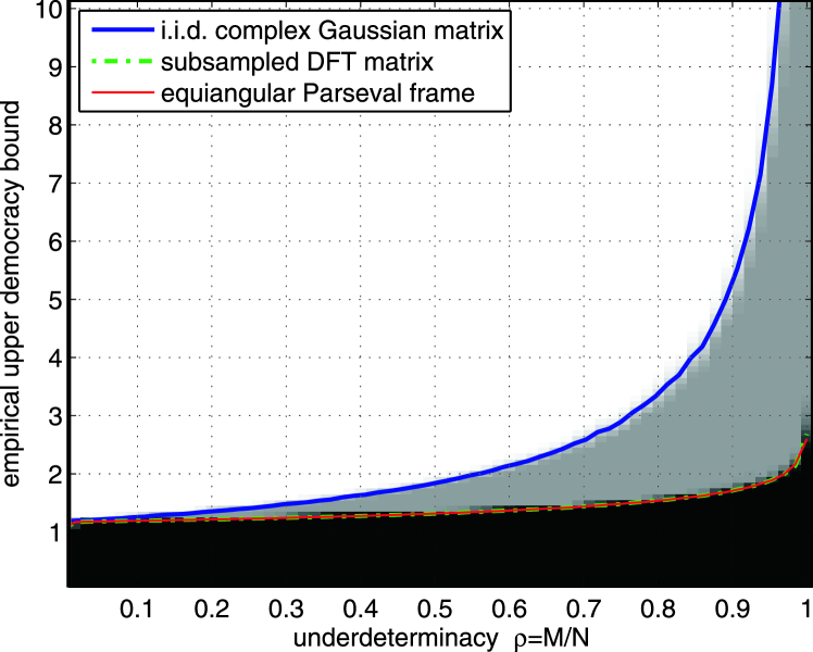
Figure 2: Empirical phase diagram depending on the underdeterminancy $\rho=M/N$ for the upper Kashin bound $K_{\text{u}}$ using $(\text{P}^{\,\varepsilon}_{\infty})$ with $\varepsilon=0$ and for (i) i.i.d. complex Gaussian matrices, (ii) randomly subsampled DFT matrices, and (iii) equiangular Parseval frames. The curves represent the individual, sharp 50% phase-transition boundaries. (Note that the curves for subsampled DFT matrices and equiangular Parseval frames overlap.)

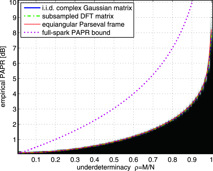
Figure 3: Empirical phase diagram depending on the underdeterminancy $\rho=M/N$ for the PAPR using $(\text{P}^{\,\varepsilon}_{\infty})$ with $\varepsilon=0$ and for (i) i.i.d. complex Gaussian matrices, (ii) randomly subsampled DFT matrices, and (iii) equiangular Parseval frames. The curves represent the individual, sharp 50% phase-transition boundaries. We also show the full-spark PAPR bound (9). (Note that the curves for i.i.d. complex Gaussian matrices, subsampled DFT matrices, and equiangular Parseval frames overlap.)

In fig:kashinbound, we show empirical phase diagrams that characterize the upper democracy bound $K_{\text{u}}$ for i.i.d. Gaussian matrices, randomly subsampled DCT matrices, and equiangular Parseval frames constructed using the algorithm of [44].

7.1.1 Simulation procedure

We fix $N=512$ and vary $M$ from 1 to 512. For each measurement/dimension pair $(N,M)$, we perform 100 Monte-Carlo trials, and for each trial we generate a frame $\mathbf{D}$ from each matrix/frame class specified above. We furthermore generate a complex i.i.d. zero-mean Gaussian vector $\mathbf{y}$ and normalize it to $\mathopen{}\left\lVert\mathbf{y}\right\rVert_{2}=1$. We use CRAMP from sec:algorithmyipee to compute signal representations $\dot{}\mathbf{x}$ from $(\text{P}^{\,\varepsilon}_{\infty})$ with $\varepsilon=0$ for each instance of $\mathbf{D}$ and $\mathbf{y}$. We then compute an empirical lower bound $\hat{K}_{\text{u}}$ on the upper democracy constant using the obtained representations $\dot{}\mathbf{x}$ for each trial as follows:

$$\hat{K}_{\text{u}}=\frac{\sqrt{N}\mathopen{}\left\lVert\dot{}\mathbf{x}\right\rVert_{\infty}}{\mathopen{}\left\lVert\mathbf{y}\right\rVert_{2}-\varepsilon}\leq K_{\text{u}}\quad\text{with}\quad\varepsilon=0.$$ (16)

We finally generate phase diagrams, which show the empirical probability for which $\hat{K}_{\text{u}}$ is larger or smaller than a given empirical upper democracy constant (given by the y-axis).

7.1.2 Discussion

The empirical phase diagram shown in fig:kashinbound shows a sharp transition between the values of $\hat{K}_{\text{u}}$ that have been realized (for a given under determinacy $\rho=M/N$) and the values that were not achieved. Moreover, we see that subsampled DFTs and equiangular Parseval frames have smaller (empirical) upper democracy constant than that of i.i.d. Gaussian matrices. This behavior is predicted by eq:maincondition and observed previously [37], and can be attributed to the fact that subsampled DFT matrices are Parseval frames, whereas i.i.d. Gaussian matrices are, in general, not tight frames (see also sec:UPsatisfyingmatrices). Hence, the use of Parseval frames tends to yield democratic representations with smaller $\ell_{\infty}$-norm than general (non-tight) frames, which is reflected by the upper democracy bound of eq:maincondition that explicitly depends on the frame bounds $A$ and $B$.

7.2 Impact of Frame Properties on PAPR

In fig:papr, we characterize the impact of frame properties on the PAPR of signal representations obtained by solving $(\text{P}^{\,\varepsilon}_{\infty})$.

7.2.1 Simulation procedure

We carry out a similar simulation procedure as in sec:simprocedure1, but instead we compute $\textit{PAPR}(\dot{}\mathbf{x})$ for each instance of $\mathbf{D}$ and $\mathbf{y}$.

7.2.2 Discussion

The phase diagram shown in fig:papr exhibits a sharp transition between the (empirical) PAPR values achieved in this simulation and the values that were not achieved. It is interesting to see that all 50% phase transitions overlap, which is in stark contrast to the transition behavior of the upper democracy bound discussed above. We, hence, conclude that the particular choice of the frame has a negligible impact for PAPR-reduction. In addition, fig:papr also shows the full-spark PAPR bound eq:parbound1. We note that the PAPR bound in thm:parbound depends on the upper frame bound $B$, which is not reflected in this simulation; an investigation of a tighter PAPR bound is part of ongoing work. Furthermore, the gap between the 50% phase transition and the full-spark PAPR bound appears to rather large. Nevertheless, we note that the full-spark PAPR bound does neither depend on the signal to be represented nor on the specifics of the used frame (apart from its dimensions). Hence, one can imagine that for certain frames one might be able to construct adversarial signals whose representations exhibit high PAPR.

7.3 Application Example: PAPR Reduction in DVB-T2

We now show a simple application example of democratic representations for PAPR reduction in an OFDM-based DVB-T2 broadcast system [29]. While this example demonstrates the efficacy of democratic representations for PAPR reduction, we do not intend to provide a thorough comparison with state-of-the-art algorithms used in real-world implementations. For a more detailed discussion on this matter, we refer the interested reader to [45, 6, 7, 8].

7.3.1 Algorithm details and simulation procedure

We consider a simplified DVB-T2 system, where we use the tones reserved for PAPR reduction to generate OFDM time-domain signals $\mathbf{x}$ having low PAPR. In particular, we generate the entries of the frequency-domain (signal) vector $\mathbf{y}$ by inserting i.i.d. random 256-QAM symbols into the data-carrying tones and by inserting $0$’s into the specified zero-tones. The set of entries in $\mathbf{y}$ containing the constellation symbols and the zero-tones is denoted by $\Omega$; the complement set $\Omega^{c}$ contains the tones reserved for PAPR reduction. We can now write the time-domain vector $\mathbf{x}$ as $\mathbf{F}\mathbf{x}=\mathbf{y}$, where $\mathbf{F}$ is a DFT matrix of appropriate size that satisfies $\mathbf{F}\mathbf{F}^{H}=\mathbf{I}$. In the following experiment, we use a DFT of dimension $N=32\,768$ as specified in [29]. For this particular DFT size, we have $\mathopen{}\left\lvert\Omega^{c}\right\rvert=288$ tones reserved for PAPR reduction. By separating the signal vector $\mathbf{y}$ into two disjoint parts $\mathbf{y}_{\Omega}$ and $\mathbf{y}_{\Omega^{c}}$, we can rewrite the time-domain vector as $\mathbf{x}=\mathbf{F}^{H}_{\Omega}\mathbf{y}_{\Omega}+\mathbf{F}^{H}_{\Omega^{c}}\mathbf{y}_{\Omega^{c}}$. Hence, for the OFDM tones in $\Omega$, we have $\mathbf{y}_{\Omega}=(\mathbf{F}^{H}_{\Omega})^{H}\mathbf{x}$; here, $(\mathbf{F}^{H}_{\Omega})^{H}$ is a subsampled DFT matrix having $M=32\,480$ rows from the set $\Omega$ and all $N=32\,768$ columns. Since $\mathbf{x}$ is the time-domain vector to be transmitted, we can reduce its PAPR by solving the following problem:

$$(\text{PR})\quad\underset{\tilde{}\mathbf{x}\in\mathbb{C}^{N}}{\text{minimize}}\,\,\mathopen{}\left\lVert\tilde{}\mathbf{x}\right\rVert_{\infty}\quad\text{subject to}\,\,\mathbf{y}_{\Omega}=(\mathbf{F}^{H}_{\Omega})^{H}\tilde{}\mathbf{x},$$

which is a specific instance of $(\text{P}^{\,\varepsilon}_{\infty})$ with $\mathbf{D}=(\mathbf{F}^{H}_{\Omega})^{H}$ and $\varepsilon=0$. By solving $(\text{PR})$ we obtain a time-domain signal $\dot{}\mathbf{x}$ that has (i) low PAPR and (ii) a frequency-domain representation that corresponds to $\mathbf{y}_{\Omega}$ on the set of used OFDM tones.

We note that, in practice, the time-domain signals pass through a digital-to-analog converter, which typically applies a low-pass reconstruction filter to the resulting time-domain signal. To accurately assess the PAPR of the resulting analog (filtered) time-domain signal, one typically considers the PAPR of an oversampled system, which is achieved by an appropriate zero-padding of frequency-domain vector $\mathbf{y}$ (see [46] and the references therein). As in [46] we compute the PAPR using $4\times$ oversampling.

In the following experiments, we generate $10^{5}$ OFDM signals $\mathbf{y}$ as specified above and compare the PAPR of the following methods/algorithms: (i) conventional OFDM transmission (where $y_{i}=0$ for $i\in\Omega^{c}$); (ii) PAPR-reduced OFDM transmission using the algorithm detailed in the DVB-T2 standard [29, Sec. 9.6.2.1]; (iii) PAPR-reduced OFDM transmission as by solving $(\text{PR})$ via CRAMP; (iv) PAPR-reducd OFDM transmission by solving a variant of $(\text{PR})$ via CRAMP that directly operates on the $4\times$ oversampled system. As a performance measure, we compare the complementary cumulative distribution function (CDF) of the oversampled PAPR values (in decibel) obtained in all simulation trials [46].

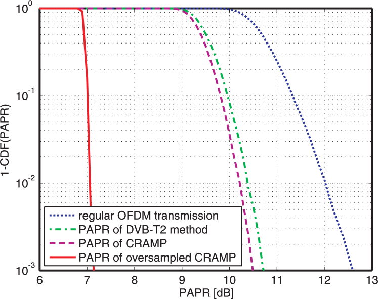
Figure 4: PAPR reduction performance for a DVB-T2-based broadcast system with 32 768 OFDM tones and 256-QAM modulation [29]. We compare the PAPR reduction performance of (i) regular OFDM transmission (no PAPR reduction use), (ii) the algorithm specified in the DVB-T2 standard, (iii) CRAMP, and (iv) CRAMP directly applied to the $4\times$ oversampled system.

7.3.2 Discussion

From fig:paprreduction, we see that conventional OFDM transmission exhibits the largest PAPR. The algorithm in [29] is able to reduce the PAPR by roughly $1.5$ dB (corresponding to a complementary CDF of $10^{-2}$). Solving $(\text{PR})$ via CRAMP reduces the PAPR by roughly $1.7$ dB. Solving $(\text{PR})$ directly on the oversampled system leads to a significant PAPR reduction of about $4.5$ dB (or $3$ dB more than conventional schemes). Hence, PAPR reduction using $\ell_{\infty}$-norm minimization is able to significantly outperform existing methods.

We conclude by noting that CRAMP-based PAPR reduction exhibits, in general, higher computational complexity than the algorithm specified in the DVB-T2 standard [29], but requires no parameter tuning. Since CRAMP does not exploit the fact that the effective matrix $(\mathbf{F}^{H}_{\Omega})^{H}$ in the considered application has a very specific structure and extremely low redundancy (i.e., $\lambda\approx 1.008$), we are convinced that more efficient algorithms can be developed for solving $(\text{PR})$ in this particular setting.

8 Conclusions

In this paper, we have analyzed a host of fundamental properties of signal representations with minimum $\ell_{\infty}$ (or maximum) norm. Specifically, we have developed properties on the magnitudes of such representations, and we characterized their peak-to-average power (PAPR) properties, which is of practical interest for OFDM-based communication systems. We have demonstrated the existence of matrices for which democratic representations with small $\ell_{\infty}$-norm and small PAPR exist. We have furthermore developed two new and computationally efficient algorithms for solving $(\text{P}^{\,\varepsilon}_{\infty})$. To support our analysis, we have conducted a set of numerical experiments, which highlight that (i) Parseval frames lead to democratic representations with smaller $\ell_{\infty}$-norm compared to general frames and (ii) democratic representations offer tremendous PAPR reduction gains over existing approaches.

There are many avenues for follow-on research. An analytical characterization of the sharp phase transitions for $(\text{P}^{\,\varepsilon}_{\infty})$ observed in sec:simkashinbound, e.g., using techniques developed in [21, 47], is an interesting open research problem. In addition, the development of algorithms particularly suited for PAPR reduction in OFDM-based communication systems is left for future work. We also believe that assessing the efficacy of democratic representations in other practical applications, such as vector quantization, approximate nearest neighbor search, filter design, or robotics and control, is an interesting research direction.

Appendix A Proof of lem:demsExist

Suppose that $\dot{}\mathbf{x}$ is a nonzero solution to $(\text{P}^{\,\varepsilon}_{\infty})$ with fewer than $N-M+1$ extreme values. Without loss of generality, suppose the first $K$ entries of $\dot{}\mathbf{x}$ are extreme, where $K<N-M+1$. Let $\dot{\mathbf{x}}_{1}$ and $\dot{\mathbf{x}}_{2}$ be the first $K$ entries and remaining entries of $\dot{}\mathbf{x}$, respectively. Similarly, let $\mathbf{D}_{1}$ be formed by the first $K$ columns of $\mathbf{D}$ and $\mathbf{D}_{2}$ be formed by its remaining $N-K$ columns. Note that $\mathbf{D}_{2}$ has $M$ rows and $N-K$ columns, where $M\leq N-K$. Hence, we have either (i) $\operatorname{rank}(\mathbf{D}_{2})=M$ or (ii) $\operatorname{rank}(\mathbf{D}_{2})<M\leq N-K$.

Case (i): $\operatorname{rank}(\mathbf{D}_{2})=M$. There exists a nonzero vector $\mathbf{v}_{2}$ such that $\mathbf{D}_{2}\mathbf{v}_{2}=\mathbf{D}\dot{\mathbf{x}}$. Let $\dot{\mathbf{y}}_{\alpha}=(1-\alpha)\dot{\mathbf{x}}+\alpha[\mathbf{0}\,;\mathbf{v}_{2}]=[(1-\alpha)\dot{\mathbf{x}}_{1}\,;(1-\alpha)\dot{\mathbf{x}}_{2}+\alpha\mathbf{v}_{2}]$. We have $\mathbf{D}\dot{\mathbf{y}}_{\alpha}=(1-\alpha)\mathbf{D}\dot{\mathbf{x}}+\alpha\mathbf{D}_{2}\mathbf{v}_{2}=(1-\alpha)\mathbf{D}\dot{\mathbf{x}}+\alpha\mathbf{D}\dot{\mathbf{x}}=\mathbf{D}\dot{\mathbf{x}}$, so $\dot{\mathbf{y}}_{\alpha}$ is a feasible solution. Since $\|\dot{\mathbf{x}}_{1}\|_{\infty}>\|\dot{\mathbf{x}}_{2}\|_{\infty}$, there exists an $\alpha>0$ such that

$$\|(1-\alpha)\dot{\mathbf{x}}_{1}\|_{\infty}=\|(1-\alpha)\dot{\mathbf{x}}_{2}+\alpha\mathbf{v}_{2}\|_{\infty}=\|\dot{\mathbf{y}}_{\alpha}\|_{\infty}<\|\dot{\mathbf{x}}\|_{\infty}.$$

We reach a contradiction that $\dot{\mathbf{y}}_{\alpha}$ is a candidate solution strictly better than $\dot{}\mathbf{x}$. Therefore, this case is impossible.

Case (ii): $\operatorname{rank}(\mathbf{D}_{2})<M\leq N-K$. There exists a nonzero vector $\mathbf{v}_{2}$ such that $\mathbf{D}_{2}\mathbf{v}_{2}=0$. Then, $\dot{\mathbf{y}}_{\alpha}=\dot{\mathbf{x}}+\alpha[\mathbf{0}\,;\mathbf{v}_{2}]=[\dot{\mathbf{x}}_{1}\,;\dot{\mathbf{x}}_{2}+\alpha\mathbf{v}_{2}]$ satisfies $\mathbf{D}\dot{\mathbf{y}}=\mathbf{D}\dot{\mathbf{x}}$ for any value of $\alpha$; thus $\dot{\mathbf{y}}_{\alpha}$ is feasible. We can select $\alpha$ such that $\|\dot{\mathbf{x}}_{2}+\alpha\mathbf{v}_{2}\|_{\infty}=\|\dot{\mathbf{x}}_{1}\|_{\infty}$ since $\|\dot{\mathbf{x}}_{2}\|_{\infty}<\|\dot{\mathbf{x}}_{1}\|_{\infty}$. Then $\|\dot{\mathbf{y}}_{\alpha}\|_{\infty}=\max\{\|\dot{\mathbf{x}}_{1}\|_{\infty},\|\dot{\mathbf{x}}_{2}+\alpha\mathbf{v}_{2}\|_{\infty}\}=\|\dot{\mathbf{x}}_{1}\|_{\infty}=\|\dot{\mathbf{x}}\|_{\infty}.$ Therefore, $\dot{\mathbf{y}}_{\alpha}$ is feasible, achieves the same objective, and has at least one more extreme value than $\dot{}\mathbf{x}$.

Appendix B Proof of lem:alwaysDem

Assume for contradiction that $(\text{P}^{\,\varepsilon}_{\infty})$ admits a solution $\dot{}\mathbf{x}$ strictly fewer than $N-M+1$ extreme values. Let $\dot{\mathbf{x}}_{1}$, $\dot{\mathbf{x}}_{2}$, $\mathbf{D}_{1}$, and $\mathbf{D}_{2}$ be defined the same as in A. Note that $\mathbf{D}_{2}$ has $M$ rows and $N-K$ columns, where $M\leq N-K$. Since $\mathbf{D}$ is a full-spark frame, $\operatorname{rank}(\mathbf{D}_{2})=M$, which is Case (i) in A and leads to a contradiction following the same arguments.

Appendix C Proof of thm:primaldualproblems

Let $\|\mathbf{w}\|_{p}$ and $\|\mathbf{v}\|_{d}$ denote the primal and dual norm of the vectors $\mathbf{w}$ and $\mathbf{x}$ satisfying

$$\|\mathbf{w}\|_{p}=\max_{\mathbf{v}}\left\{\Re\big{(}\mathbf{v}^{H}\mathbf{w}\big{)}\colon\!\|\mathbf{v}\|_{d}\leq 1\right\}$$

with $1/p+1/d=1$ and $p,d\geq 1$. Then, for primal and dual norms, we have the following result [39]:

$$\min_{\mathbf{x}}\left\{\|\mathbf{x}\|_{p}\!-\!\Re\big{(}\mathbf{z}^{H}\mathbf{D}\mathbf{x}\big{)}\right\}=\left\{\begin{array}[]{ll}0,&\|\mathbf{D}^{H}\mathbf{z}\|_{d}\leq 1\\[5.69046pt] -\infty,&\text{otherwise}.\end{array}\right.$$ (19)

We are now ready to derive the Lagrange dual problem $(\text{D}^{\,\varepsilon}_{p})$ to the primal problem $(\text{P}^{\,\varepsilon}_{p})$. To this end, we introduce the auxiliary vector $\mathbf{r}\in\mathbb{C}^{M}$ to rewrite $(\text{P}^{\,\varepsilon}_{p})$ as

$$\min_{\mathbf{x}}\left\{\|\mathbf{x}\|_{p}\colon\mathopen{}\left\lVert\mathbf{D}\mathbf{x}-\mathbf{y}\right\rVert_{2}\leq\varepsilon\right\}$$

$$\quad\qquad=\min_{\mathbf{x},\mathbf{r}}\left\{\|\mathbf{x}\|_{p}\colon\mathbf{D}\mathbf{x}+\mathbf{r}=\mathbf{y},\mathopen{}\left\lVert\mathbf{r}\right\rVert_{2}\leq\varepsilon\right\}.$$

By introducing the Lagrange dual variable $\mathbf{z}\in\mathbb{C}^{M}$, we obtain

$$\min_{\mathbf{x},\mathbf{r}}\left\{\|\mathbf{x}\|_{p}\colon\mathbf{D}\mathbf{x}+\mathbf{r}=\mathbf{y},\mathopen{}\left\lVert\mathbf{r}\right\rVert_{2}\leq\varepsilon\right\}$$

$$=\min_{\mathbf{x},\mathbf{r}}\max_{\mathbf{z}}\left\{\|\mathbf{x}\|_{p}\!-\!\Re\big{(}\mathbf{z}^{H}(\mathbf{D}\mathbf{x}\!+\!\mathbf{r}\!-\!\mathbf{y})\big{)}\colon\!\mathopen{}\left\lVert\mathbf{r}\right\rVert_{2}\leq\varepsilon\right\}$$

$$=\max_{\mathbf{z}}\min_{\mathbf{x},\mathbf{r}}\left\{\|\mathbf{x}\|_{p}\!-\!\Re\big{(}\mathbf{z}^{H}(\mathbf{D}\mathbf{x}\!+\!\mathbf{r}\!-\mathbf{y})\big{)}\colon\!\mathopen{}\left\lVert\mathbf{r}\right\rVert_{2}\leq\varepsilon\right\}\!.$$ (20)

For a given $\mathbf{z}$, the inner minimization problem of eq:primaldualproblems_step1 is separable in the unknown vectors $\mathbf{x}$ and $\mathbf{r}$. The optimal auxiliary vector $\mathbf{r}$ is given by

$$\mathbf{r}=\left\{\begin{array}[]{ll}\varepsilon\mathbf{z}/\mathopen{}\left\lVert\mathbf{z}\right\rVert_{2},&\mathbf{z}\neq\mathbf{0}_{M\times 1}\\[5.69046pt] \mathbf{0}_{M\times 1},&\text{otherwise},\end{array}\right.$$

and, in either case, we have $\Re\big{(}\mathbf{z}^{H}\mathbf{r}\big{)}=\varepsilon\mathopen{}\left\lVert\mathbf{z}\right\rVert_{2}$. Together with eq:primaldualproblems_step0, we find that eq:primaldualproblems_step1 is equal to

$$\max_{\mathbf{z}}\left\{\Re\big{(}\mathbf{y}^{H}\mathbf{z}\big{)}-\varepsilon\mathopen{}\left\lVert\mathbf{z}\right\rVert_{2}\colon\|\mathbf{D}^{H}\mathbf{z}\|_{d}\leq 1\right\}\!,$$

which corresponds to the Lagrange dual problem $(\text{D}^{\,\varepsilon}_{p})$. Note that since in the derivation of $(\text{D}^{\,\varepsilon}_{p})$ all intermediate steps hold with equality, there is no duality gap.

Appendix D Proof of lem:lowerkashinbound

The proof follows from a lower bound on the value of the dual problem $(\text{D}^{\,\varepsilon}_{\infty})$. Specifically, we have

$$\mathopen{}\left\lVert\dot{}\mathbf{x}\right\rVert_{\infty}=\max_{\mathbf{z}}\left\{\Re\!\left(\mathbf{y}^{H}\mathbf{z}\right)-\varepsilon\mathopen{}\left\lVert\mathbf{z}\right\rVert_{2}\colon\mathopen{}\left\lVert\mathbf{D}^{H}\mathbf{z}\right\rVert_{1}\leq 1\right\}\!,$$ (21)

which we bound from below by replacing the optimal solution $\dot{}\mathbf{z}$ by the following feasible solution:

$$\hat{}\mathbf{z}=\frac{\mathbf{y}}{\mathopen{}\left\lVert\mathbf{D}^{H}\mathbf{y}\right\rVert_{1}},$$ (22)

which satisfies the constraint $\mathopen{}\left\lVert\mathbf{D}^{H}\hat{}\mathbf{z}\right\rVert_{1}\leq 1$. Hence, inserting eq:lower_step2 in the right-hand side (RHS) of eq:lower_step1 leads to the following lower bound:

$$\mathopen{}\left\lVert\dot{}\mathbf{x}\right\rVert_{\infty}\geq\frac{\mathopen{}\left\lVert\mathbf{y}\right\rVert_{2}^{2}-\varepsilon\mathopen{}\left\lVert\mathbf{y}\right\rVert_{2}}{\mathopen{}\left\lVert\mathbf{D}^{H}\mathbf{y}\right\rVert_{1}}.$$ (23)

To further bound the RHS of eq:lower_step3 from below, we use standard norm bounds and the upper frame bound $B$ of $\mathbf{D}$ to compute an upper bound to $\mathopen{}\left\lVert\mathbf{D}^{H}\mathbf{y}\right\rVert_{1}$ as follows:

$$\mathopen{}\left\lVert\mathbf{D}^{H}\mathbf{y}\right\rVert_{1}\leq\sqrt{N}\mathopen{}\left\lVert\mathbf{D}^{H}\mathbf{y}\right\rVert_{2}\leq\sqrt{NB}\mathopen{}\left\lVert\mathbf{y}\right\rVert_{2}.$$ (24)

Combining eq:lower_step4 with eq:lower_step3 finally yields

$$\mathopen{}\left\lVert\dot{}\mathbf{x}\right\rVert_{\infty}\geq\frac{\mathopen{}\left\lVert\mathbf{y}\right\rVert_{2}-\varepsilon}{\sqrt{NB}}.$$ (25)

Note that in eq:lower_step2 we assumed that $\mathopen{}\left\lVert\mathbf{D}^{H}\mathbf{y}\right\rVert_{1}>0$. Since $\mathbf{D}$ is a frame with lower frame bound $A>0$, we have

$$\mathopen{}\left\lVert\mathbf{D}^{H}\mathbf{y}\right\rVert_{1}\geq\mathopen{}\left\lVert\mathbf{D}^{H}\mathbf{y}\right\rVert_{2}\geq\sqrt{A}\mathopen{}\left\lVert\mathbf{y}\right\rVert_{2}>0,$$

which is satisfied whenever $\mathopen{}\left\lVert\mathbf{y}\right\rVert_{2}>0$. In the case $\mathopen{}\left\lVert\mathbf{y}\right\rVert_{2}=0$ the bound eq:lower_step5 continues to hold.

Appendix E Proof of thm:main_result

The proof proceeds in two stages. First, we separate the objective function of the Lagrange dual problem $(\text{D}^{\,\varepsilon}_{\infty})$ into two independent terms and second, we derive an upper bound on the $\ell_{2}$-norm of the solution $\dot{}\mathbf{z}$ to $(\text{D}^{\,\varepsilon}_{\infty})$.

E.1 Separating the Result of the Lagrange Dual Problem

From the Lagrange dual problem $(\text{D}^{\,\varepsilon}_{\infty})$, we have

$$\mathopen{}\left\lVert\dot{}\mathbf{x}\right\rVert_{\infty} =\Re\!\left(\mathbf{y}^{H}\dot{}\mathbf{z}\right)-\varepsilon\mathopen{}\left\lVert\dot{}\mathbf{z}\right\rVert_{2}\leq\mathopen{}\left\lvert\mathbf{y}^{H}\dot{}\mathbf{z}\right\rvert-\varepsilon\mathopen{}\left\lVert\dot{}\mathbf{z}\right\rVert_{2}$$

$$\leq\mathopen{}\left\lVert\dot{}\mathbf{z}\right\rVert_{2}\!\left(\mathopen{}\left\lVert\mathbf{y}\right\rVert_{2}-\varepsilon\right),$$ (26)

as an immediate consequence of the Cauchy-Schwarz inequality. In the remaining steps of the proof, we derive an upper bound on $\mathopen{}\left\lVert\dot{}\mathbf{z}\right\rVert_{2}$ in eq:main_step1. To this end, we first expand

$$\mathopen{}\left\lVert\dot{}\mathbf{z}\right\rVert_{2}=\mathopen{}\left\lVert(\mathbf{D}\mathbf{D}^{H})^{-1}\mathbf{D}\mathbf{D}^{H}\dot{}\mathbf{z}\right\rVert_{2},$$ (27)

where $\mathbf{D}\mathbf{D}^{H}$ is invertible since $\mathbf{D}$ is a frame with lower frame bound satisfying $A>0$. Application of the Rayleigh-Ritz theorem [48, Thm. 4.2.2] to the right-hand side (RHS) of (27) leads to the following upper bound:

$$\mathopen{}\left\lVert\dot{}\mathbf{z}\right\rVert_{2}\leq\mathopen{}\left\lVert(\mathbf{D}\mathbf{D}^{H})^{-1}\right\rVert_{2,2}\mathopen{}\left\lVert\mathbf{D}\mathbf{D}^{H}\dot{}\mathbf{z}\right\rVert_{2}\leq\frac{1}{A}\mathopen{}\left\lVert\mathbf{D}\mathbf{D}^{H}\dot{}\mathbf{z}\right\rVert_{2},$$ (28)

where the second inequality is a result of

$$\mathopen{}\left\lVert(\mathbf{D}\mathbf{D}^{H})^{-1}\right\rVert_{2,2}=\frac{1}{\mathopen{}\left\lVert(\mathbf{D}\mathbf{D}^{H})^{-1}\right\rVert_{2,2}}\leq\frac{1}{A}$$

and the assumption that $\mathbf{D}$ is a frame with lower frame bound $A>0$. We next derive an upper bound on $\mathopen{}\left\lVert\mathbf{D}\mathbf{D}^{H}\mathbf{z}\right\rVert_{2}$ in eq:main_step2.

Note that one can straightforwardly arrive at an upper bound on $\mathopen{}\left\lVert\dot{}\mathbf{x}\right\rVert_{\infty}$ as follows:

$$\mathopen{}\left\lVert\mathbf{D}\mathbf{D}^{H}\dot{}\mathbf{z}\right\rVert_{2} \leq\mathopen{}\left\lVert\mathbf{D}\right\rVert_{2,2}\mathopen{}\left\lVert\mathbf{D}^{H}\dot{}\mathbf{z}\right\rVert_{1}\leq\mathopen{}\left\lVert\mathbf{D}\right\rVert_{2,2}$$ (29)

using $\mathopen{}\left\lVert\mathbf{D}^{H}\dot{}\mathbf{z}\right\rVert_{2}\leq\mathopen{}\left\lVert\mathbf{D}^{H}\dot{}\mathbf{z}\right\rVert_{1}$ and the constraint $\mathopen{}\left\lVert\mathbf{D}^{H}\dot{}\mathbf{z}\right\rVert_{1}\leq 1$ of the dual problem $(\text{D}^{\,\varepsilon}_{\infty})$. Hence, by combining eq:main_step1, eq:main_step2, and eq:main_step2b one would arrive at the following result:

$$\mathopen{}\left\lVert\dot{}\mathbf{x}\right\rVert_{\infty}\leq\frac{\mathopen{}\left\lVert\mathbf{D}\right\rVert_{2,2}}{A}\big{(}\mathopen{}\left\lVert\mathbf{y}\right\rVert_{2}-\varepsilon\big{)}.$$ (30)

This bound is, however, overly pessimistic and does not exploit additional properties of the frame $\mathbf{D}$. Note that for Parseval frames, the result eq:main_step2b_crap leads to the bound $\mathopen{}\left\lVert\dot{}\mathbf{x}\right\rVert_{\infty}\leq\mathopen{}\left\lVert\mathbf{y}\right\rVert_{2}-\varepsilon$.

E.2 Refined Upper Bound

In order to arrive at a refined bound on $\mathopen{}\left\lVert\mathbf{D}\mathbf{D}^{H}\dot{}\mathbf{z}\right\rVert_{2}$, we define an $N$-dimensional vector $\mathbf{v}=\mathbf{D}^{H}\dot{}\mathbf{z}$ and divide its coefficients into $S=\lceil 1/\delta\rceil$ disjoint support sets, each of cardinality $\delta N$ such that

$$\Omega_{1}\cup\cdots\cup\Omega_{\ell}\in\{1,\ldots,N\},$$

where $\lceil x\rceil$ rounds the scalar $x\in\mathbb{R}$ to the nearest integer towards infinity. Moreover, the magnitudes of the entries in $\mathbf{v}$ associated to set $\Omega_{\ell}$ are no smaller than the magnitudes associated with the sets $\Omega_{k}$, $k>\ell$. In other words, $\Omega_{1}$ contains the indices associated to the largest $\delta N$ entries in $\mathbf{v}$, $\Omega_{2}$ the $\delta N$ coefficients associated to the second largest entries, etc. This partitioning scheme now allows us to rewrite $\mathopen{}\left\lVert\mathbf{D}\mathbf{D}^{H}\dot{}\mathbf{z}\right\rVert_{2}$ as

$$\mathopen{}\left\lVert\mathbf{D}\mathbf{D}^{H}\dot{}\mathbf{z}\right\rVert_{2}=\mathopen{}\left\lVert\mathbf{D}\sum_{i=1}^{S}\mathbf{P}_{\Omega_{i}}\mathbf{D}^{H}\dot{}\mathbf{z}\right\rVert_{2},$$

where the matrix $\mathbf{P}_{\Omega_{i}}$ realizes a projection onto the set $\Omega_{i}$. Application of the triangle inequality, followed by using properties of the UP with parameters $\eta$, $\delta$ leads to the following:

$$\mathopen{}\left\lVert\mathbf{D}\mathbf{D}^{H}\dot{}\mathbf{z}\right\rVert_{2} \leq\sum_{i=1}^{S}\mathopen{}\left\lVert\mathbf{D}\mathbf{P}_{\Omega_{i}}\mathbf{D}^{H}\dot{}\mathbf{z}\right\rVert_{2}\leq\sum_{i=1}^{S}\eta\mathopen{}\left\lVert\mathbf{P}_{\Omega_{i}}\mathbf{D}^{H}\dot{}\mathbf{z}\right\rVert_{2}$$

$$=\eta\mathopen{}\left\lVert\mathbf{P}_{\Omega_{1}}\mathbf{D}^{H}\dot{}\mathbf{z}\right\rVert_{2}+\sum_{i=2}^{S}\eta\mathopen{}\left\lVert\mathbf{P}_{\Omega_{i}}\mathbf{D}^{H}\dot{}\mathbf{z}\right\rVert_{2}.$$ (31)

Since the sets $\Omega_{i}$ order the entries of $\mathbf{v}=\mathbf{D}^{H}\dot{}\mathbf{z}$ according to their magnitudes, we can use a technique developed in [49], which states that for $i\in\{2,\ldots,S\}$ we have

$$\mathopen{}\left\lVert\mathbf{P}_{\Omega_{i}}\mathbf{v}\right\rVert_{2}\leq\sqrt{\delta N}\mathopen{}\left\lVert\mathbf{P}_{\Omega_{i}}\mathbf{v}\right\rVert_{\infty}\leq\frac{1}{\sqrt{\delta N}}\mathopen{}\left\lVert\mathbf{P}_{\Omega_{i-1}}\mathbf{v}\right\rVert_{1}.$$

This result in combination with the RHS of (31) leads to

$$\mathopen{}\left\lVert\mathbf{D}\mathbf{D}^{H}\dot{}\mathbf{z}\right\rVert_{2} \leq\eta\mathopen{}\left\lVert\mathbf{P}_{\Omega_{1}}\mathbf{D}^{H}\dot{}\mathbf{z}\right\rVert_{2}+\sum_{i=1}^{S}\frac{\eta}{\sqrt{\delta N}}\mathopen{}\left\lVert\mathbf{P}_{\Omega_{i}}\mathbf{D}^{H}\dot{}\mathbf{z}\right\rVert_{1}$$

$$=\eta\mathopen{}\left\lVert\mathbf{P}_{\Omega_{1}}\mathbf{D}^{H}\dot{}\mathbf{z}\right\rVert_{2}+\frac{\eta}{\sqrt{\delta N}}\mathopen{}\left\lVert\mathbf{D}^{H}\dot{}\mathbf{z}\right\rVert_{1}$$

$$=\eta\mathopen{}\left\lVert\mathbf{P}_{\Omega_{1}}\mathbf{D}^{H}\dot{}\mathbf{z}\right\rVert_{2}+\frac{\eta}{\sqrt{\delta N}},$$ (32)

where the first equality follows from the fact that $\mathopen{}\left\lVert\mathbf{D}^{H}\dot{}\mathbf{z}\right\rVert_{1}\leq 1$ for any solution $\dot{}\mathbf{z}$ to the dual problem $(\text{D}^{\varepsilon}_{\infty})$.

We can now bound the first RHS term in eq:main_step4 as

$$\mathopen{}\left\lVert\mathbf{P}_{\Omega_{1}}\mathbf{D}^{H}\dot{}\mathbf{z}\right\rVert_{2}\leq\mathopen{}\left\lVert\mathbf{D}^{H}\dot{}\mathbf{z}\right\rVert_{2}\leq\sqrt{B}\mathopen{}\left\lVert\dot{}\mathbf{z}\right\rVert_{2}$$ (33)

using the facts that (i) $\mathbf{P}_{\Omega_{1}}$ is a projector and (ii) $\mathbf{D}$ is a frame with (upper) frame bound $B$. By combining eq:main_step2, eq:main_step4, and eq:main_step5 we arrive at

$$\mathopen{}\left\lVert\dot{}\mathbf{z}\right\rVert_{2} \leq\frac{1}{A}\!\left(\eta\sqrt{B}\mathopen{}\left\lVert\dot{}\mathbf{z}\right\rVert_{2}+\frac{\eta}{\sqrt{\delta N}}\right),$$

which can be rewritten as

$$\mathopen{}\left\lVert\dot{}\mathbf{z}\right\rVert_{2} \leq\frac{\eta}{(A-\eta\sqrt{B})\sqrt{\delta N}}$$ (34)

provided that $A>\eta\sqrt{B}$ holds. Combining eq:main_step1 with eq:main_step5b finally yields

$$\mathopen{}\left\lVert\dot{}\mathbf{x}\right\rVert_{\infty} \leq\frac{\eta}{(A-\eta\sqrt{B})\sqrt{\delta N}}\big{(}\mathopen{}\left\lVert\mathbf{y}\right\rVert_{2}-\varepsilon\big{)},$$ (35)

which concludes the proof. We finally note that eq:main_step6 is able to scale in $1/\sqrt{N}\mathopen{}\left\lVert\mathbf{y}\right\rVert_{2}$ for certain frames (see sec:UPsatisfyingmatrices).

Appendix F Proof of thm:parbound

The proof follows from separately bounding the numerator and denominator of the definition eq:pardefinition. We first bound $N\mathopen{}\left\lVert\dot{}\mathbf{x}\right\rVert_{\infty}^{2}$ using eq:maincondition to arrive at

$$N\mathopen{}\left\lVert\dot{}\mathbf{x}\right\rVert_{\infty}^{2}\leq\widetilde{K}_{\text{u}}^{2}(\mathopen{}\left\lVert\mathbf{y}\right\rVert_{2}-\varepsilon)^{2}.$$ (36)

The second part of the proof bounds $\mathopen{}\left\lVert\dot{}\mathbf{x}\right\rVert_{2}^{2}$ from below. To this end, it is important to realize that

$$\mathopen{}\left\lVert\dot{}\mathbf{x}\right\rVert_{2}\geq\min_{\mathbf{x}}\left\{\mathopen{}\left\lVert\mathbf{x}\right\rVert_{2}\colon\!\mathopen{}\left\lVert\mathbf{y}-\mathbf{D}\mathbf{x}\right\rVert_{2}\leq\varepsilon\right\}$$ (37)

because $\dot{}\mathbf{x}$ satisfies $\mathopen{}\left\lVert\mathbf{y}-\mathbf{D}\dot{}\mathbf{x}\right\rVert_{2}\leq\varepsilon$ and the RHS is the minimizer for all vectors $\mathbf{x}\in\mathbb{C}^{N}$ satisfying $\mathopen{}\left\lVert\mathbf{y}-\mathbf{D}\mathbf{x}\right\rVert_{2}\leq\varepsilon$. We next compute a lower bound on the RHS of eq:parbound_step1. From thm:primaldualproblems with $p=2$ and $q=2$, we have

$$\min_{\mathbf{x}}\left\{\mathopen{}\left\lVert\mathbf{x}\right\rVert_{2}\colon\!\mathopen{}\left\lVert\mathbf{y}-\mathbf{D}\mathbf{x}\right\rVert_{2}\leq\varepsilon\right\}$$

$$\qquad=\max_{\mathbf{z}}\left\{\Re\big{(}\mathbf{y}^{H}\mathbf{z}\big{)}-\varepsilon\mathopen{}\left\lVert\mathbf{z}\right\rVert_{2}\colon\!\mathopen{}\left\lVert\mathbf{D}^{H}\mathbf{z}\right\rVert_{2}\leq 1\right\}.$$ (38)

Using a similar strategy as in app:lowerkashinbound, we replace the optimal solution $\dot{}\mathbf{z}$ of the dual problem in eq:parbound_step1a by the estimate

$$\dot{}\mathbf{z}=\frac{\mathbf{y}}{\mathopen{}\left\lVert\mathbf{D}^{H}\mathbf{y}\right\rVert_{2}},$$ (39)

which satisfies the constraint $\mathopen{}\left\lVert\mathbf{D}^{H}\mathbf{y}\right\rVert_{2}\leq 1$. Hence, by inserting the estimate eq:parbound_step2 into the RHS of eq:parbound_step1a, we obtain the following lower bound:

$$\max_{\mathbf{z}}\left\{\Re\big{(}\mathbf{y}^{H}\mathbf{z}\big{)}-\varepsilon\mathopen{}\left\lVert\mathbf{z}\right\rVert_{2}\colon\!\mathopen{}\left\lVert\mathbf{D}^{H}\mathbf{z}\right\rVert_{2}\leq 1\right\}$$

$$\qquad\geq\frac{\mathopen{}\left\lVert\mathbf{y}\right\rVert_{2}^{2}-\varepsilon\mathopen{}\left\lVert\mathbf{y}\right\rVert_{2}}{\mathopen{}\left\lVert\mathbf{D}^{H}\mathbf{y}\right\rVert_{2}}.$$ (40)

The upper frame bound $\mathopen{}\left\lVert\mathbf{D}^{H}\mathbf{y}\right\rVert_{2}\leq\sqrt{B}\mathopen{}\left\lVert\mathbf{y}\right\rVert_{2}$ enables us to further bound the RHS of eq:parbound_step3 from below as

$$\frac{\mathopen{}\left\lVert\mathbf{y}\right\rVert_{2}^{2}-\varepsilon\mathopen{}\left\lVert\mathbf{y}\right\rVert_{2}}{\mathopen{}\left\lVert\mathbf{D}^{H}\mathbf{y}\right\rVert_{2}}\geq\frac{\mathopen{}\left\lVert\mathbf{y}\right\rVert_{2}-\varepsilon}{\sqrt{B}}.$$ (41)

By combining eq:parbound_step1, eq:parbound_step1a, eq:parbound_step3, and eq:parbound_step5, we finally obtain

$$\mathopen{}\left\lVert\dot{}\mathbf{x}\right\rVert_{2}^{2}\geq\frac{\big{(}\mathopen{}\left\lVert\mathbf{y}\right\rVert_{2}-\varepsilon\big{)}^{2}}{B}.$$ (42)

Consequently, if $\varepsilon<\mathopen{}\left\lVert\mathbf{y}\right\rVert_{2}$, then we can bound the PAPR of the representation $\dot{}\mathbf{x}$ obtained from $(P^{\,\varepsilon}_{\infty})$ using eq:parbound_step0 and eq:parbound_step6 as $\textit{PAPR}(\dot{}\mathbf{x})\leq\widetilde{K}_{\text{u}}^{2}B$. Note that in eq:parbound_step2 we assumed that $\dot{}\mathbf{x}\neq 0$, i.e., we require $A>0$ and $\mathopen{}\left\lVert\mathbf{y}\right\rVert_{2}\neq 0$.

Appendix G Proof of thm:gainbound

For the lower bound in eq:powerincrease, we simply recall the fact that the $\ell_{2}$-norm of the LS solution $\mathopen{}\left\lVert\hat{}\mathbf{x}\right\rVert_{2}$ is, by definition of the optimization problem $(\text{P}^{\,\varepsilon}_{2})$, smaller than the $\ell_{2}$-norm of a democratic representation $\mathopen{}\left\lVert\dot{}\mathbf{x}\right\rVert_{2}$. Consequently, we get the trivial bound $\textit{PI}=\mathopen{}\left\lVert\dot{}\mathbf{x}\right\rVert_{2}^{2}/\mathopen{}\left\lVert\hat{}\mathbf{x}\right\rVert_{2}^{2}\geq 1$.

To arrive at the upper bound in eq:powerincrease, we follow closely the proof in app:parbound and individually bound the numerator and denominator of eq:powerincrease. First, we bound $\mathopen{}\left\lVert\dot{}\mathbf{x}\right\rVert_{2}^{2}$ from above as

$$\mathopen{}\left\lVert\dot{}\mathbf{x}\right\rVert_{2}^{2}\leq N\mathopen{}\left\lVert\dot{}\mathbf{x}\right\rVert_{\infty}^{2}\leq\widetilde{K}_{\text{u}}^{2}(\mathopen{}\left\lVert\mathbf{y}\right\rVert_{2}-\varepsilon)^{2},$$ (43)

which is a consequence of standard norm bounds and the results of eq:kashinbounds and eq:maincondition. We next obtain a lower bound on the denominator $\mathopen{}\left\lVert\hat{}\mathbf{x}\right\rVert_{2}^{2}$ of eq:powerincrease. To this end, we carry out the steps in eq:parbound_step1a–eq:parbound_step6 for $\mathopen{}\left\lVert\hat{}\mathbf{x}\right\rVert_{2}^{2}$ to arrive at the following lower bound:

$$\mathopen{}\left\lVert\hat{}\mathbf{x}\right\rVert_{2}^{2}\geq\frac{\big{(}\mathopen{}\left\lVert\mathbf{y}\right\rVert_{2}-\varepsilon\big{)}^{2}}{B}.$$

Finally, combining eq:gainbound_step1 with eq:gainbound_step1 yields $\textit{PI}\leq\widetilde{K}_{\text{u}}^{2}B$. We conclude by noting that the steps in eq:parbound_step1a–eq:parbound_step6 require $\mathopen{}\left\lVert\mathbf{y}\right\rVert_{2}\neq 0$, $A>0$, and $\varepsilon<\mathopen{}\left\lVert\mathbf{y}\right\rVert_{2}$.

References

- [1] Y. Lyubarskii, R. Vershynin, Uncertainty principles and vector quantization, IEEE Trans. Inf. Theory 56 (7) (2010) 3491–3501.
- [2] J.-J. Fuchs, Spread represenations, in: Proc. 45th Asilomar Conf. on Signals, Systems, and Comput., Pacific Grove, CA, USA, 2011.
- [3] A. R. Calderbank, I. Daubechies, The pros and cons of democracy, IEEE Trans. Inf. Theory 48 (6) (2002) 1721–1725.
- [4] M. Püschel, J. Kovačević, Real, tight frames with maximal robustness to erasures, in: Proc. IEEE Data Compression Conf. (DDC), 2005, pp. 63–72.
- [5] C. Novak, C. Studer, A. Burg, G. Matz, The effect of unreliable LLR storage on the performance of MIMO-BICM, in: Proc. of 44th Asilomar Conf. on Signals, Systems, and Comput., Pacific Grove, CA, USA, 2010, pp. 736–740.
- [6] R. van Nee, R. Prasad, OFDM for wireless multimedia communications, Artech House Publ., 2000.
- [7] J. Illic, T. Strohmer, PAPR reduction in OFDM using Kashin’s representation, in: Proc. IEEE 10th Workshop on Sig. Proc. Advances in Wireless Comm. (SPAWC), Perugia, Italy, 2009, pp. 444–448.
- [8] C. Studer, E. G. Larsson, PAR-aware large-scale multi-user MIMO-OFDM downlink, IEEE J. Sel. Areas Comm. 31 (2) (2013) 303–313.
- [9] H. Jégou, T. Furon, J.-J. Fuchs, Anti-sparse coding for approximate nearest neighbor search, arXiv:1110.3767v2.
- [10] J. A. Cadzow, Algorithm for the minimum-effort problem, IEEE Trans. Autom. Control. 16 (1) (1971) 60–63.
- [11] A. S. Deo, I. D. Walker, Minimum effort inverse kinematics for redundant manipulators, IEEE Trans. Robotics and Automation 13 (5) (1997) 767–775.
- [12] Y. Zhang, J. Wang, Y. Xu, A dual neural network for bi-criteria kinematic control of redundant manipulators, IEEE Trans. Robotics and Automation 18 (6) (2002) 923–931.
- [13] H. Zhang, M. Yan, W. Yin, One conition for all: solution uniqueness and robustness of -synthesis and -analysis minimizations, CAAM Technical Report 13-10, Rice University (Apr. 2013).
- [14] J. A. Tropp, Greed is good: Algorithmic results for sparse approximation, IEEE Trans. Inf. Theory 50 (10) (2004) 2231–2242.
- [15] M. Elad, Sparse and Redundant Representations: From Theory to Applications in Signal and Image Processing, 1st Edition, Springer, 2010.
- [16] C. Studer, R. G. Baraniuk, Stable restoration and separation of approximately sparse signals, Appl. Comput. Harmon. Anal.
- [17] D. L. Donoho, Compressed sensing, IEEE Trans. Inf. Theory 52 (4) (2006) 1289–1306.
- [18] E. J. Candès, J. Romberg, T. Tao, Robust uncertainty principles: Exact signal reconstruction from highly incomplete frequency information, IEEE Trans. Inf. Theory 52 (2) (2006) 489–509.
- [19] E. J. Candès, M. B. Wakin, An introdutction to compressive sampling, IEEE Sig. Proc. Mag. 25 (2) (2008) 21–30.
- [20] R. G. Baraniuk, M. Davenport, R. A. DeVore, M. B. Wakin, A simple proof of the restricted isometry property for random matrices, Constr. Approx. 28 (2008) 253–263.
- [21] D. L. Donoho, J. Tanner, Precise undersampling theorems, Proc. of the IEEE 98 (6) (2010) 913–924.
- [22] O. Mangasarian, B. Recht, Probability of unique integer solution to a system of linear equations, Europ. J. of Operational Research 214 (1) (2011) 27–30.
- [23] V. Chandrasekaran, B. Recht, P. A. Parrilo, A. S. Willsky, The convex geometry of linear inverse problems, Foundations of Computational mathematics 12 (6) (2012) 805–849.
- [24] S. Oymak, C. Thrampoulidis, B. Hassibi, Simple bounds for noisy linear inverse problems with exact side information, arXiv preprint:1312.0641.
- [25] L. W. Neustadt, Minimum effort control systems, J. Soc. Indus. and Appl. Math. Ser 1 (1) (1962) 16–31.
- [26] B. Kashin, Sections of some finite dimensional sets and classes of smooth functions, Izv. Acad. Nauk SSSR 41 (2) (1977) 334–351.
- [27] A. Y. Garnaev, E. D. Gluskin, On widths of the Euclidean ball, Soviet Math. Dokl. 30 (1) (1984) 200–204.
- [28] E. J. Candès, T. Tao, Near-optimal signal recovery from random projections and universal encoding strategies?, IEEE Trans. Inf. Theory 52 (2006) 5406–5425.
- [29] ETSI EN 302 755, Digital video broadcasting (DVB); frame structure channel coding and modulation for a second generation digital terrestrial television broadcasting system (DVB-T2), Tech. rep., Version 1.3.1 (Apr. 2012).
- [30] D. Seethaler, H. Bölcskei, Performance and complexity analysis of infinity-norm sphere-decoding, IEEE Trans. Inf. Theory 56 (3) (2010) 1085–1105.
- [31] V. I. Morgenshtern, H. Bölcskei, A short course on frame theory, CRC Press, Chapter in Mathematical Foundations for Signal Processing, Communications, and Networking, 2012.
-
[32]
B. Alexeev, J. Cahill, D. Mixon,