The PdBI Arcsecond Whirlpool Survey (PAWS):
Multi-phase cold gas kinematic of M51

Abstract

The kinematic complexity and the favorable position of M51 on the sky make this galaxy an ideal target to test different theories of spiral arm dynamics. Taking advantage of the new high resolution PdBI Arcsecond Whirlpool Survey (PAWS) data, we undertake a detailed kinematic study of M51 to characterize and quantify the origin and nature of the non-circular motions. Using a tilted-ring analysis supported by several other archival datasets we update the estimation of M51’s position angle ($PA=(173\pm 3)^{\circ}$) and inclination ($i=(22\pm 5)^{\circ}$). Harmonic decomposition of the high resolution ($\sim 40$ pc) CO velocity field shows the first kinematic evidence of an $m=3$ wave in the inner disk of M51 with a corotation at $R_{CR,m=3}=1.1\pm 0.1$ kpc and a pattern speed of $\Omega_{p,m=3}\approx 140$ km s^-1 kpc^-1. This mode seems to be excited by the nuclear bar, while the beat frequencies generated by the coupling between the $m=3$ mode and the main spiral structure confirm its density-wave nature. We observe also a signature of an $m=1$ mode that is likely responsible for the lopsidedness of M51 at small and large radii. We provide a simple method to estimate the radial variation of the amplitude of the spiral perturbation ($V_{sp}$) attributed to the different modes. The main spiral arm structure has $\langle V_{sp}\rangle=50-70$ km s^-1, while the streaming velocity associated with the $m=1$ and $m=3$ modes is, in general, 2 times lower. Our joint analysis of HI and CO velocity fields at low and high spatial resolution reveals that the atomic and molecular gas phases respond differently to the spiral perturbation due to their different vertical distribution and emission morphology.

1 Introduction

Gas kinematics are key to dissecting how the various components of a galaxy (stars, gas and dust) interact and evolve over time, leading to the variety of morphologies we see in the local universe today. They supply the standard for probing the mass distributions of galaxies through rotation curves and are uniquely sensitive to perturbations to the gravitational potential due to bars and spiral arms (Roberts & Stewart 1987; Vogel et al. 1993; Regan et al. 2001; Dobbs et al. 2010). By providing an instantaneous record of the response of gas to non-axisymmetric (bar and spiral) structures, they supply a unique view of the processes by which these features impact the distribution of gas and stars, from stimulating stellar radial migration (Sellwood & Binney 2002; Minchev et al. 2012) and driving gas inflows (Wong et al. 2004; van de Ven & Fathi 2010) to regulating the conversion of gas into stars (Meidt et al. 2013). Gas kinematics are therefore indispensable for building a firm picture of how bar and spiral structures contribute to the slow, secular evolution of galaxies.

Studying the response of gas to an underlying potential perturbation (in the form of bars or spiral arms) can supply key information about the nature of the perturbation (e.g. Vogel et al. 1993; Wong et al. 2004). Today, spiral structures tend to be described by one of two opposite theories. In the quasi-stationary spiral structure (QSSS) depiction (Lindblad 1963), spiral arms are a long lasting pattern (Lin & Shu 1964) that slowly evolves and rotates with a single angular speed. This structure is thought to be formed from self-excited and self-regulated standing “density waves” (Bertin et al. 1989a; Bertin et al. 1989b; Bertin & Lin 1996) present in the density and hence gravitational potential. The other theory considers arms to be transient disturbances generated, e.g., by the tidal interaction with a companion (e.g., Toomre & Toomre 1972) which overwhelms any pre-existing structure (Salo & Laurikainen 2000) or given some initial seed perturbation (D’Onghia et al. 2013). These structures, which may not obey the Lin-Shu dispersion relation for density waves (Salo & Laurikainen 2000, D’Onghia et al. 2013), are often thought to be winding (with radially decreasing pattern speeds) or to consist of material moving at series of distinct speeds.

Most of the effort to discriminate between these two theories has been centered on M51, which is an ideal target because of its proximity (D=7.6 Mpc, Ciardullo et al. 2002), favorable inclination ($i\sim 22^{\circ}$, this work), high surface brightness and kinematic complexity. In the seminal M51 kinematic study of Tully (1974), the spiral pattern in the outer disk was identified as a transient feature stimulated by the interaction between M51a and M51b, while the inner arms were thought to be in a steady state. Indeed, Vogel et al. (1993) find very good agreement between the predictions of density-wave theory and the observed transverse velocities across the inner arms. But more recently, Shetty et al. (2007) argue that gas density and velocity profiles are inconsistent with quasi-steady state mass conservation.

At least some of the ambiguity regarding the nature of M51’s spiral pattern may stem from the complexity of its structure. Meidt et al. (2008) found evidence for three distinct pattern speeds in M51 using the radial Tremaine-Weinberg (TWR) method, only one of which is similar to the value typically assumed. Their finding that these patterns overlap at resonances would seem to be consistent with the idea that they are physically coupled and not temporary disturbances. But multiple, distinct pattern speeds may also support the D’Onghia et al. (2013) picture wherein a disturbance drives a transient feature that stimulates other transient features, which together give the appearance of long-lived structures.

The disk of M51 may also sustain multiple, spatially coincident patterns. The optical and NIR surface brightness is clearly lopsided, suggesting an $m=1$ disturbance in the potential. This lopsidedness persists in tracers of the ISM. Some part of the lopsidedness could be explained by the superposition of the two-armed spiral with a spiral pattern with three-fold symmetry (Henry et al. 2003). The existence of such a pattern in M51 was first suggested between radii of 50” and 100” in blue light optical images by Elmegreen et al. (1992). Rix & Rieke (1993) also find the signature of a three-armed pattern in the K-band, although at a much weaker level than in the V-band. Both studies conclude that the $m=3$ feature in M51 is a perturbation in the gas and dust only (traced in extinction at optical and NIR wavelengths), rather than a genuine density wave present in the density (traced by the old stellar light) and thus gravitational potential of the system, although this idea was later challenged by Henry et al. (2003). As pointed out by Elmegreen et al. (1992), simple Fourier transforms of galaxy images can provide misleading results on the nature and number of spiral arms if they are not confirmed by kinematic evidence. The $m$=3 component, for example, could arise as a beat frequency, modulated by inter-arm star formation or by an intensity gradient from one side of the galaxy to the other (due to extinction or kinematic effects).

In this paper we take advantage of the new high resolution ¹²CO (1-0) PAWS observations in the central 9 kpc of M51. The high resolution of this data ($\sim 1"$) allows us to perform an in-depth study of the gas response to M51’s perturbed stellar potential. If the $m=3$ mode is a genuine perturbation to the potential then our high resolution map of molecular gas motions should reveal it. We complement our kinematic analysis with lower resolution HI and ¹²CO (2-1) data from THINGS (Walter et al. 2008) and HERACLES (Schuster et al. 2004, Leroy et al. 2009). The inclusion of observations of various phases of the ISM, at low and high resolution, allows us to assess how uniformly they trace the gravitational potential, and determine which type of observational tracer is optimal for which science goal. The 21 cm and the CO line emission are the common tracers of the atomic and the molecular gas phases that are at the basis of star formation. To understand the physics behind empirical laws that relate gas and stars from kpc (e.g. Leroy et al. 2013, Bigiel et al. 2008 and references therein) to pc scales it is necessary to constrain their characteristics at every level, especially how they are distributed within, and respond to the potential of, a given system.

The paper is constructed in the following way. In Section 2 we present the datasets used for our kinematic analysis. Then we describe the features of the high resolution velocity field from PAWS in Section 3. We introduce the formalism to study the line-of-sight velocity ($V_{los}$) in spiral galaxies in Section 4 together with our estimation of the projection parameters of M51 (inclination and position angle) needed for a correct evaluation of the single component of $V_{los}$. In Section 5 we use the harmonic decomposition prescriptions to study residual velocity fields. We propose a method to estimate the amplitude of the perturbation velocity from the spiral arms and we present the first kinematic evidence for a three-fold density-wave in M51. We conclude in Section 6 discussing the origin of this structure and highlighting kinematic differences between atomic and molecular gas tracers and low and high resolution data (Section 7). We summarize our work and findings in Section 8.

2 Data

2.1 PAWS ¹²CO(1-0) data

The PdBI Arcsecond Whirlpool Survey (PAWS, Schinnerer et al. 2013) “hybrid cube” considered here has been obtained by combining the IRAM-30m single-dish antenna and Plateau de Bure Interferometer (PdBI) ¹²CO(1-0) observations of M51 (Pety et al. 2013). The cube has an angular resolution of $1^{\prime\prime}.16\times 0^{\prime\prime}.97$ (or $\sim 40$ pc at $7.6$ Mpc distance, Ciardullo et al. 2002), a mean RMS noise of $\sim 0.4$ K per 5 km s^-1 channel and covers the LSR velocity range between 173 to 769 km s^-1. PdBI dedicated observations of the inner disk of M51a (field-of-view, FoV $\sim 270^{\prime\prime}\times 170^{\prime\prime}$ or $\sim 11\times 6$ kpc) were carried out in the A, B, C, and D configurations from August 2009 and March 2010.

We also independently consider the 30m single-dish observations (hereafter indicated with the name 30m) of the full disk of M51 ($\sim 60$ square arcminutes) conducted to recover the low spatial frequency information filtered out by the PdBI. This data has a spatial resolution of $22.5"$ (i.e. $\sim 900$ pc at 7.6 Mpc distance) and a channel width of $\sim 5$ km s^-1.

To study the impact of resolution, we also include the hybrid data cubes gaussian-tapered to a synthesized resolution of 3” and 6” presented in Pety et al. (2013) with typical RMS noise of 0.1 and 0.03 K, respectively. These PAWS datasets span the same range of LSR velocities and have the same field-of-view as the PAWS dataset at 1”.

2.2 Archival THINGS VLA HI data

M51 HI data from The HI Nearby Galaxy Survey (THINGS, Walter et al. 2008) was obtained from the dedicated web-page http://www.mpia-hd.mpg.de/THINGS/Data.html. M51 was observed between March 2005 and July 2007 using the NRAO Very Large Array (VLA) in B, C and D configuration. The robust-weighted THINGS data used here has a spatial resolution of $\sim 6"$ (i.e. 240 pc at our assumed M51 distance of 7.6 Mpc) and a spectral resolution of $\sim 5$ km s^-1. The $1\sigma_{RMS}$ noise sensitivity of the survey is homogeneous and $\sim 6$ K per channel. We use this data together with the PAWS data to better define the rotation curve of M51, as it covers the entire disk of M51a.

2.3 Archival HERACLES IRAM 30m ¹²CO(2-1) data

The Heterodyne Receiver Array CO Line Extragalactic Survey (HERACLES, Leroy et al. 2009) re-reduced and mapped the data previously obtained for M51 by Schuster et al. (2004) using the HERA receiver array on the IRAM 30m telescope from January 2006 through March 2008 for M51. The ¹²CO (2-1) M51 data has a spatial resolution of $\sim 13.5"$ (540 pc in M51) and a spectral resolution of $\sim 2.6$ km s^-1. M51 data presents an $1\sigma_{RMS}$ noise sensitivity $\sim 22$ mK per channel.

3 M51a neutral gas velocity fields

In the following we will utilize the moment maps (velocity field, velocity dispersion map) derived for our different neutral gas cubes following the masking method described in the Appendix B of Pety et al. (2013). The PAWS 1” velocity field (top left of Fig 1) exhibits significant deviations from pure circular motion (visible in the irregularity of line-of-nodes), the most prominent of which are: strong spiral arm streaming motions, a twist in the central region and the nucleus of M51a itself.

The streaming motions associated with the spiral arms are particularly evident in the southern half of the PAWS FoV, characterized by discontinuities and velocity gradients across the arm. The deviation persists to a much lesser degree in parts of the inter-arm region. Streaming motions appears less strong in the northern compared to the southern half.

In the central region ($R\lesssim 35"$) the iso-velocity contours are strongly twisted by $10-15^{\circ}$. A recent torque analysis (Meidt et al. 2013) suggests that the observed twisting is due to the nuclear bar first seen in near-IR images (Zaritsky et al. 1993). At the very center of the map, the nuclear gas shows a clear out-of-velocity pattern redshifted by $\approx 100$ km s^-1 with respect to the systemic velocity (see also Scoville et al. 1998, Matsushita et al. 2007).

The prominence of these features is reduced at degraded resolution, as they are largely smeared out by a larger beam. To illustrate this, in Fig. 1 we show the first moment maps from PAWS tapered at 6”, THINGS at 6” and HERACLES at 13.5”. In PAWS 6” the redshifted nucleus is not visible and the discontinuities of the velocity gradient across the arms are strongly reduced. These features are completely absent in the THINGS and HERACLES first moment maps. While in the case of HERACLES this absence could be due to the much lower resolution and the lack of interferometric data, the difference between the CO and HI data at the same resolution could be due to a real difference in the nature and distribution of the two emission line tracers. We discuss this possibility in Section 7.

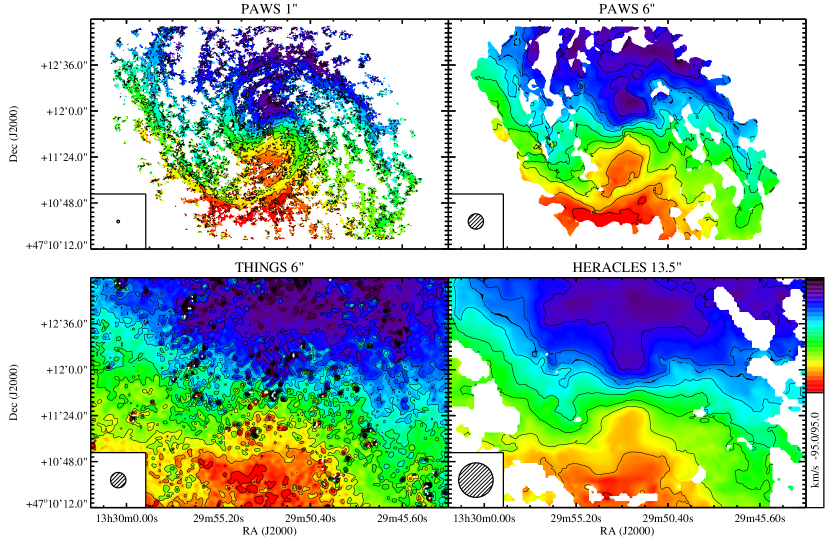
Figure 1: The PAWS ¹²CO(1-0) Velocity field at 1” resolution (top left). Deviations from circular motion are due to streaming motions associated with the spiral arms and the nuclear stellar bar which causes the twist in the inner line-of-nodes. M51’s nucleus is also redshifted with respect to the systemic velocity of the galaxy. These features are progressively smeared out by the beam in the PAWS tapered 6” (top right), THINGS 6” (bottom left) and HERACLES 13.5” (bottom right) velocity fields. The sidebar shows the color scale of the map in km s^-1 relative to the systemic velocity of M51, 472 km s^-1 (Shetty et al. 2007). In the bottom left of each panel the beam is indicated (where 1”$\sim 40$ pc).

4 Gas motions in spiral potentials

In this section and the next, we consider the different velocity components that contribute along the line-of-sight in a typical spiral galaxy in the presence of strong non-circular motions. Each component is analyzed in detail in order to gain an optimal view of cold gas kinematics in M51, as well as to explore how this view depends on the resolution at which the gas motions are observed.

4.1 Line-of-sight velocity

The line-of-sight velocity $V_{los}$ observed at a given location in a galactic disk can be represented as a sum of four parts:

$$V_{los}=V_{sys}+V_{rot}+V_{pec}+V_{z}$$ (1)

where $V_{sys}$ is the systemic velocity of the galaxy due to the expansion of the Universe, $V_{rot}$ is the rotational component, $V_{pec}$ represents all peculiar velocities not accounted for the circular motion of the galaxy and $V_{z}$ is the vertical velocity component (i.e. Canzian & Allen 1997). Studies of face-on grand-design spirals indicate that $V_{z}$ of the neutral gas is less than 5 km s^-1 (van der Kruit & Shostak 1982), in which case $V_{los}$ can be well represented by planar motion without considerable vertical motions. Therefore throughout this paper we assume $V_{z}\equiv 0$.

The rotational component can be expressed as

$$V_{rot}=V_{c}\cos(\theta)\sin i,$$ (2)

where $V_{c}$ is the circular rotation speed, $\theta$ is the angle in the plane of the disk from the major-axis receding side, and $i$ represents the inclination of the disk to the plane of the sky. (The inclination $i$ is equal to $0^{\circ}$ for an exactly face-on galaxy and $i=90^{\circ}$ for a completely edge-on geometry.)

In a grand-design spiral galaxy such as M51, the peculiar component is largely due to the gas response to the density wave perturbation, i.e.

$$V_{pec}=(u_{\phi}\cos\theta+u_{r}\sin\theta)\sin i$$ (3)

where $u_{r}$ and $u_{\psi}$ are the (non-circular) radial and azimuthal components of streaming motions.

4.2 Kinematic parameter estimation

Our main goal in this paper is to measure and analyze the streaming motions in the inner disk of M51. To correctly interpret the line-of-sight projections of peculiar motions (i.e. $V_{pec}$) we must therefore first have a good knowledge of the kinematic parameters that describe the projection of the galaxy on the plane of the sky. Several parameters are already well-constrained in the literature and do not require further analysis (Section 4.2.1). For others, we provide new estimations – with uncertainties (Section 4.2.2) – applying a tilted-ring analysis to the different velocity fields from PAWS 1”, PAWS 3”, THINGS 6”, HERACLES 13.5” and 30m at 22.5”.

4.2.1 Previous M51 kinematic studies

Because of its proximity, favourable inclination and prominent spiral arms, M51 has been the focus of a large number of kinematic studies aimed at testing theories of spiral arm formation and evolution. A summary of those focused on the determination of the kinematic parameters is provided in Tables 1-2.

In general the systemic velocity of M51 is well-constrained around a value $V_{sys}=472$ km s^-1. Therefore, in the following we adopt the literature value for this quantity (e.g. Shetty et al. 2007).

The center of M51, corresponding to the location of the nucleus, has been carefully constrained by measurements of H₂O maser emission and high resolution radio continuum imaging (see Table 2 and references therein). Throughout this paper we adopt as rotation center the latest measurement of the water maser by Hagiwara (2007), i.e. $(x_{0},y_{0})=(13^{h}29^{m}52^{s}.71,47^{\circ}11^{\prime}42".79)$. The adopted rotation center almost coincides with the peak of CO emission associated with M51a’s bright core (located at $(x_{core},y_{core})=(13^{h}29^{m}52^{s}.62,47^{\circ}11^{\prime}42".58)$), clearly identifiable only by PAWS at 1”.

Estimates for the position angle $PA$ and inclination $i$ span a large range in the literature (see Table 1 and references therein), between PA=$165-180^{\circ}$ and $i$= $15-28^{\circ}$. With the aim of updating these estimates and providing a tighter constraint, in the next section we apply a tilted-ring analysis to the most recent high-resolution gas velocity fields available for M51 from the THINGS, HERACLES and PAWS projects.

Table 1: M51a (NGC 5194) kinematic parameters measured by previous studies

Resolution	Tracer	$V_{sys}$	$PA$	$i$	Reference
2”/4”	H$\alpha$/12CO(1-0)	$471.7\pm 0.3$	$175\pm 5$	$24\pm 3$	(1)
4”	12CO(1-0)	$469$	$170\pm 5$	…	(2)
5”	H$\alpha$	$470\pm 2$	…	…	(3)
6”	HI	…	…	30	(4)
6”.75	H$\alpha$	$472\pm 3$	$170\pm 3$	$20\pm 5$	(5)
16”	12CO(1-0)	$469\pm 5$	$171.6$	…	(6)

Note. — (1), Shetty et al. (2007); (2), Meidt et al. (2008); (3), Goad et al. (1979); (4), de Blok et al. (2008); (5), Tully (1974); (6) Kuno & Nakai (1997). In Shetty et al. (2007) and Meidt et al. (2008), 4” refers to the best resolution of the BIMA-SONG data used.

Table 2: Center of M51a (NGC 5194) as derived from previous studies

Resolution	Method	$x_{0},y_{0}$	Reference
$\sim$0”.1	H2O maser spot	$13^{h}29^{m}52^{s}.71,47^{\circ}11^{\prime}42".79$	(1)
$\sim$0”.1	H2O maser spot	$13^{h}29^{m}52^{s}.71,47^{\circ}11^{\prime}42".80$	(2)
1”	6-20 cm continuum peak	$13^{h}29^{m}52^{s}.70,47^{\circ}11^{\prime}42".60$	(3)
1”.1	6 cm radio continuum peak	$13^{h}29^{m}52^{s}.71,47^{\circ}11^{\prime}42".61$	(4)
$\sim$1”.3	6-20 cm continuum peak	$13^{h}29^{m}52^{s}.71,47^{\circ}11^{\prime}42".73$	(5)
…	Optical measurement	$13^{h}29^{m}53^{s}.27,47^{\circ}11^{\prime}48".36$	(6)

Note. — (1), Hagiwara (2007); (2), Hagiwara et al. (2001); (3), Ford et al. (1985); (4), Turner & Ho (1994); (5), Maddox et al. (2007); (6), Dressel & Condon (1976). (B1950) coordinates reported by several studies have been converted to (J2000) using NED.

4.2.2 Tilted-ring analysis

To quantify the kinematic parameters of M51a we assume that the various quantities of Eq. 1 vary only with galactocentric radius $R$. In this case, the first moment of the line-of-side velocity distribution can be studied through a standard tilted ring approach (Rogstad et al. 1974). We perform a least-square tilted-ring fit to the line-of-sight velocity field using the GIPSY task ROTCUR, sampling the velocity field at one radial bin per synthesized beam width from a starting radius of one half-beam.

We implement a two step procedure to obtain estimates of M51a’s kinematic parameters ($i$, $PA$):

• First we fix the systemic velocity and rotational center using the literature values discussed in Section 4.2.1, i.e. $V_{sys}=472$ km s^-1 and ($x_{0},y_{0}$)=($13^{h}29^{m}52.41^{s}$, $47^{\circ}11^{\prime}42.80"$), and $V_{rad}=0$ but leaving free inclination $i$, position angle $PA$ and rotation velocity $V_{rot}$. We estimate the magnitude of $\langle PA\rangle$ and $\langle i\rangle$ as weighted medians along the radial profile, using the inverse of the squared-errors calculated directly by ROTCUR as weights. These errors are typically larger at large galactocentric radius where the data sampling is lower.

• In the second step we set different values of inclination (i.e. $20^{\circ}$, $23^{\circ}$, $25^{\circ}$, $27^{\circ}$, $30^{\circ}$, $33^{\circ}$, $35^{\circ}$, $37^{\circ}$, $40^{\circ}$, $45^{\circ}$) to obtain our final position angle. For every fixed inclination we calculate the weighted median as a function of radius. Then we apply this same procedure to obtain the inclination itself, fixing different values of $PA$ (i.e. $165^{\circ}$, $167^{\circ}$, $170^{\circ}$, $172^{\circ}$, $173^{\circ}$, $174^{\circ}$, $175^{\circ}$, $177^{\circ}$, $180^{\circ}$, $185^{\circ}$).

The final results of the two steps are summarized in Table 3. Alongside our analysis of the PAWS 1” and 3” velocity fields, we perform the tilted ring analysis of the 6” THINGS HI velocity field (Walter et al. 2008), the HERACLES ¹²CO(2-1) first moment map at 13.5” (Leroy et al. 2009) and the 30m data at 22.5” (Pety et al. 2013). These maps all extend beyond the PAWS field of view and allow us to sample the full disk of M51a. Compared to the hybrid PAWS data, these maps should also be less sensitive to the contribution of non-circular streaming motions, which are progressively smeared out the lower the angular resolution. As described in Section 3, strong spiral arm streaming motions cause distortions in the iso-velocity contours in the PAWS velocity field at 1” (see Figure 1-2), which influence the estimate of the position angle. Tilted-ring solutions from these independent data sets with a larger field-of-view also provide a much-needed consistency check on estimates from the PAWS data, given that the close to face-on orientation can make it difficult to reliably assess the kinematic parameters.

Table 3: Kinematic parameters from the tilted-ring analysis

Map	Step	$\mathbf{\langle i\rangle}$	$\mathbf{\langle PA\rangle}$
		$[deg]$	$[deg]$
PAWS 1”	1	$48\pm 7$	$177\pm 4$
	2	$45\pm 8$	$177\pm 4$
PAWS 3”	1	$54\pm 8$	$176\pm 5$
	2	$48\pm 10$	$177\pm 4$
THINGS 6”	1	$30\pm 12$	$172\pm 2$
	2	$22\pm 5$	$173\pm 3$
HERACLES 13.5”	1	$30\pm 6$	$171\pm 4$
	2	$25\pm 7$	$172\pm 4$
30m 22.5”	1	$35\pm 4$	$174\pm 2$
	2	$22\pm 3$	$171\pm 4$

Note. — Weighted median and median absolute deviation (MAD) of kinematic parameters (inclination $\langle i\rangle$, position angle $\langle PA\rangle$) derived for each survey following the two steps described in the text.

In all data sets, we find that the position angle of M51a is fairly robust to changes in the assumed inclination. The PA is more sensitive to the presence of streaming motions, however. While we find $\langle PA\rangle\sim 170^{\circ}-173^{\circ}$ from the low resolution data where the influence of the streaming motion is reduced (i.e. from 30m, HERACLES or THINGS data), the $\langle PA\rangle$ increases to $\sim 176^{\circ}$ for the PAWS data at 1” and 3” resolution.

Streaming motions also influence the inclination estimates, which we find to be especially sensitive to the assumed position angle (yielding larger error bars). Considering that the strongest streaming motions in M51 appear in the central 5 kpc and weaken at larger galactocentric radius (where the outer spiral pattern is weaker), the FoV of a given survey largely determines the value of the inclination that can be retrieved. For maps with large FoV (30m, HERACLES and THINGS) the inclination is low ($\langle i\rangle\sim 22^{\circ}-25^{\circ}$), while for PAWS at 1” covering a smaller FoV, the average inclination is higher than $40^{\circ}$. We note that our tilted ring analysis avoids the outer warp in M51 (as obvious in the HI distribution). Since we sample the maps with large FOVs only up to the start of the warp, our inclination and position angles are representative of the disk.

Since the THINGS HI survey has the largest FoV and probes the (outer) part of the disk where we expect a lesser contribution from streaming motions, we adopt estimates from this data as our final, best measurements of the kinematic parameters: i.e. $\langle i\rangle=(22\pm 5)^{\circ}$ and $\langle PA\rangle=(173\pm 3)^{\circ}$. These exhibit the smallest error bars and the most constant behavior for various set values of $PA$ and $i$, respectively (Step 2). These results are consistent with the most recent measurements of the projection parameters performed by Hu et al. 2013, ($PA=(168.0\pm 2.5)^{\circ}$, $i=(20.3\pm 2.8)^{\circ}$), using a parametrization of M51’s spiral arms imaged in $i-$band by the SDSS (Data Release 9). The more constant behavior of the $PA$ and $i$ indicated by the HI compared to CO datasets might also reflect the different natures of the atomic and molecular gas phases (see Section 7).

5 Non-circular motions

As is clear by a simple examination of the PAWS velocity field, gas motions in M51 deviate strongly from pure circular motion. The non-axisymmetric stellar bar and spiral arms drive strong radial and azimuthal “streaming” motions, which contribute to the term $V_{pec}$ in Eq. 1 and become apparent when removing a circular velocity model from the observed velocity field.

In the following we analyze the peculiar motions that are not described by the model of pure circular motion. We start by summarizing the main features in the residual velocity field, obtained by subtracting a 2D projected model of the best estimate of $V_{c}$ from the observed velocity field. Then we describe and investigate in detail the residual velocity field and its features using a harmonic decomposition (Schoenmakers et al. 1997). Finally, we use the results of the harmonic decomposition to estimate the amplitude of the spiral arm streaming motions.

5.1 Residual velocity fields

Adopting the rotation curve from Meidt et al. (2013), we generate a 2D model of pure circular motion using the GIPSY task VELFI. This model is subtracted from the observed velocity fields to obtain residual fields for PAWS at 1”, shown in Fig 2, and for the 30m, HERACLES and THINGS velocity fields, shown in Fig. 3. In the case of pure circular motion the residuals would be zero everywhere. But here, residual velocity fields from each of the different surveys exhibit clear signatures of significant non-circular motions, with typical values between -30 and 30 km s^-1 and extrema reaching values above 90 km s^-1 (corresponding to the nucleus). In presence of density-wave structures, the non-circular motions introduce a particular morphological pattern in the residual velocity field, as realized by Canzian (1993). In the case of a m=2 perturbation to the gravitational potential (introduced by a two-armed stellar spiral or a stellar bar), the residual velocity field exhibits an m=1 pattern (i.e. an approaching-receding dipole) inside corotation, and this changes to an m=3 morphology outside corotation. This morphology shift is due to the change in sign of the gas streaming motions beyond the corotation circle, affecting only their radial components, and is expected to appear at the corotation only if the spiral structure is density-wave in nature with a constant pattern speed.

Although the pattern predicted by Canzian (1993) can be difficult to distinguish at lower spatial resolution, the residual velocity fields from the PAWS data at 1” and 3” resolution (top of Fig. 2) show the signature very clearly, over several radial zones. In the central region ($R<35"$) the residual velocity field presents a clear m=1 pattern consistent with motions driven by the m=2 stellar nuclear bar. Just outside the molecular ring at R=23” and up until $R\approx$55”, we see another approaching-receding dipole, now introduced by inflow motions driven by the two-armed spiral in this region (especially clear at the location of the southern spiral arm). This is complimented by transition to an m=3 pattern beyond $R<$55”, although between this radius and $R\lesssim 70"$ the morphology becomes more complex. In the outermost region ($R\gtrsim 70"$), where the density-wave spiral transitions to material spiral arms (Meidt et al. 2013), the PAWS FoV exhibits only a dipole.

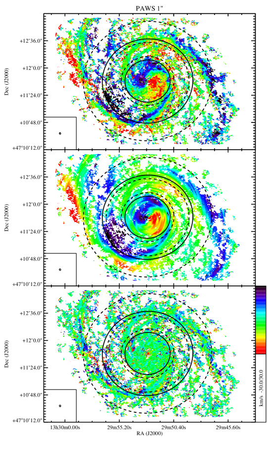
Figure 2: Top: from left to right, PAWS 1” residual velocity field. The inner dashed black circle indicates the outer boundary of the molecular ring ($R=35"$). The outer black dashed circles mark the radial location of the first corotation at $R=55"$ and the material arms at $R=85"$ as identified through the present-day torque analysis by Meidt et al. (2013). The solid black circles indicate the corotation identified with the harmonic decomposition at $R=30"$ and $R=60"$. Individual pixels within the residual velocity fields exhibit values between and km s^-1, but we restrict the color stretch to values between -30 and +30 km s^-1 to highlight the main features of the residual velocity field. $\sim 95\%$ of pixels have values that fall within the range [-30, 30] km s^-1. Middle: Harmonic reconstructed residual velocity field. Bottom: Difference between the observed residual velocity field and its harmonic reconstruction. The beam is indicated in the bottom left of each panel.

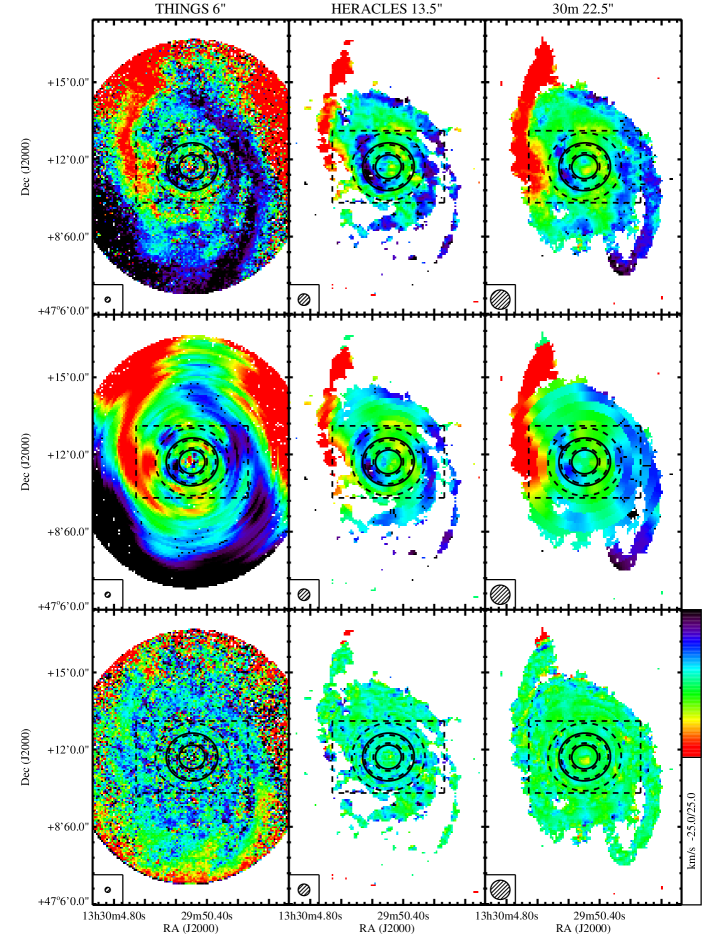
Figure 3: Top: from left to right, residual velocity fields from THINGS HI, HERACLES ¹²CO(2-1) and 30m ¹²CO(1-0). The inner dashed black circle indicates the outer boundary of the molecular ring ($R=35"$). The outer black dashed circles mark the radial location of the first corotation at $R=55"$ and the material arms at $R=85"$ as identified through the present-day torque analysis by Meidt et al. (2013). The solid black circles indicate the corotation identified with the harmonic decomposition at $R=30"$ and $R=60"$. Individual pixels within the residual velocity fields exhibit values between and km s^-1, but we restrict the color stretch to values between -25 and +25 km s^-1 to highlight the main features of the residual velocity field. $\sim 95\%$ of pixels have values that fall within the range [-25, 25] km s^-1. Middle: Harmonic reconstructed residual velocity field. Bottom: Difference between the observed residual velocity field and its harmonic reconstruction. The beam is indicated in the bottom left of each panel.

5.2 Harmonic decomposition of the non-circular velocity component

In the previous section we identified several kinematic features not associated with pure circular motion.

Here we use a powerful technique first introduced by Schoenmakers et al. (1997) to describe and quantify non-circular motions, namely by expanding the peculiar component of the line-of-sight velocity $V_{pec}$ as the harmonic series

$$V_{pec}=\sum_{j=1}^{N}[c_{j}\cos(j\theta)+s_{j}\sin(j\theta)]\sin(i),$$ (4)

Here $N$ is the number of harmonics considered and $c_{j}$ and $s_{j}$ are coefficients that describe the radial and azimuthal components of the non-circular motion, which can be interpreted in terms of perturbations to the gravitational potential. Canzian (1993) showed that a potential perturbation of $m$ order introduces $j=m-1$ and $j=m+1$ patterns in the residual velocity field, each on either side of the pattern’s corotation radius (see the upcoming section).

We quantify the magnitude, or power, of each individual order of the harmonic decomposition $j$ as the quadratically-added amplitude (e.g. Trachternach et al. 2008):

$$A_{j}=\sqrt{c_{j}^{2}+s_{j}^{2}}.$$ (5)

and write the total power of all non-circular harmonic components as

$$A_{r}=\sqrt{\Sigma_{j=1}^{N}[c_{j}^{2}+s_{j}^{2}]},$$ (6)

to get a sense of the total magnitude of non-circular streaming motions. In the next section we inspect radial trends in $A_{j}$ and $A_{r}$ for coincidence with morphological features in M51. Later in Section 5.5.1 we use our measurements of $A_{j}$ to calculate the magnitude of the streaming motions associated with perturbations with $m$-fold symmetry.

5.2.1 Application to residual velocity fields

We perform the harmonic decomposition of the residual velocity field from PAWS at 1”, PAWS 3”, THINGS, HERACLES, and 30m velocity field up to order $j=6$ using a modified version of the code first presented in Fathi et al. (2005). The inclination and PA of the best fitting ellipses are fixed to the values derived in Section 4.2 ($i=22^{\circ}$, $PA=173^{\circ}$) and the ring width is set to one beam. Fig 2 and Fig 3 shows the residual velocity fields reconstructed from the harmonic decomposition (middle row). Since the difference between residual velocity fields and the reconstructed fields is generally close to zero everywhere (Fig 2 and Fig 3, bottom row) we are confident that the harmonic decomposition using only 6 terms is quite accurate.

In Fig. 4, 10 and 11 we plot the power in the single harmonic components, and their total, as a function of radius (bottom plot, top left and top right columns), the median of these across the environments defined in Meidt et al. (2013) (e.g. nuclear bar, molecular ring, density-wave spiral arm and material arm regions; top plot, bottom left and bottom right columns) and the median across the FoV (top plot). The error bars shown there are obtained through a bootstrap technique. We generate 100 residual velocity fields, and 100 harmonic decompositions, for a range of PA and $i$ (set to their respective error bars). We take the results determined at our optimal $PA=173^{\circ}$ and $i=22^{\circ}$ as our final estimate and define the error on that estimate as the median absolute deviation of the bootstrapped amplitudes.

To discriminate between real trends and noisy peaks in the harmonic decompositions, we set a confidence level at $2\times$ the channel width of the survey (i.e. 10 km s^-1 or in the case of HERACLES 5.2 km s^-1). The (azimuthally averaged) harmonic components are highly reliable when they are above this threshold.

5.3 Global Trends

As expected, surveys with high spatial resolution reveal larger streaming motions than those with lower resolution. In PAWS 1” and PAWS 3” data the global amplitude of the non-circular components is $\langle A_{r}\rangle$$\sim 45$ km s^-1, whereas $\langle A_{r}\rangle\sim 20-35$ km s^-1  for the low resolution surveys, even when restricting the FoV to the PAWS FoV. This difference stems from the fact that contributions from motions induced by the nuclear bar and spiral arms are not well resolved in these other surveys.

However all surveys, independent of resolution, very clearly show the signature of a dominant two-armed pattern. As predicted by Canzian (1993) the expected $j=1$ and $j=3$ modes induced by the bar and two-armed spiral in M51 are apparent in all surveys: $j=1$ is the dominant mode of the residuals ($\langle A_{1}\rangle\approx 30$ km s^-1 for PAWS and $\langle A_{1}\rangle\approx 10-20$ km s^-1 for the low resolution surveys, approaching the total power within maps restricted to the PAWS FoV), followed by the $j=3$ mode ($\langle A_{3}\rangle\approx 20$ km s^-1 for PAWS and $\langle A_{3}\rangle\approx 10-15$ km s^-1 for the low resolution surveys). However in all cases, the $j=2$ mode has a value quite close to the $j=3$ ($\langle A_{2}\rangle\approx 12$ km s^-1 for PAWS and HERACLES maps and $\langle A_{2}\rangle\approx 10$ km s^-1 for THINGS and PAWS single dish). A non-negligible $j=2$ velocity term would indicate a possible $m=1$ or $m=3$ perturbation to the galactic potential. However this is difficult to confirm from global measurements since, on average, perturbations of order $j>3$ all have amplitudes $<10$ km s^-1. Given that individual components may or may not extend as far as the dominant two-armed spiral (that spans the entire field of view), below we explore the evidence for $m=1$ and $m=3$ modes by analyzing radial trends.

5.4 Radial Trends

The high resolution of the PAWS data (at either 1” or 3”) provides the most accurate depiction of the radial variation in the different harmonic components (at least for radii $R<85"$). We therefore focus on these data in this Section, but note similar trends when present in the lower resolution survey data.

5.4.1 Odd velocity modes: the bar and two-armed spiral arms

The innermost region of M51 ($R<23.5"$) is dominated by the peculiar motions driven by the nuclear bar, which introduces a $j=1$ mode between 2 to 3 times stronger than the other modes in this zone ($\langle A_{r}^{(R<23.5")}\rangle\sim\langle A_{1}^{(R<23.5")}\rangle\sim 35$ km s^-1). Just outside the bar, in the zone of the molecular ring ($23.5"<R<35"$), the peculiar motions are reduced, reaching their lowest values across the FoV ($A_{r}^{(23.5"<R<35")}\sim 20$ km s^-1 and $A_{1}^{(23.5"<R<35")}\sim 10$ km s^-1). However, near $R$=35” the $j=1$ term begins to increase again ($\langle A_{3}^{(23.5"<R<35")}\rangle\sim 40$ km s^-1). After $R\sim$60” the power in the $j$=3 mode also once again increases, to a level comparable to that in the $j$=1 mode.

Here the harmonic expansion confirms the visual impression from the residual velocity field morphology analysis: inside the torque-based estimate of the first spiral arm corotation radius ($R_{CR}=55"$, Meidt et al. 2013) the residual velocity field appears dominated by a dipole pattern ($\langle A_{1}^{(35"<R<55")}\rangle\sim 40$ km s^-1 and $\langle A_{3}^{(35"<R<55")}\rangle\sim 15$ km s^-1), while beyond the $j=3$ term is stronger ($\langle A_{1}^{(55"<R<85")}\rangle\sim 10$ km s^-1 and $\langle A_{3}^{(55"<R<85")}\rangle\sim 50$ km s^-1) and then reduces to $\sim 10$ km s^-1 in the region $(65"<R<80")$. The switch in dominance from $j$=1 to $j$=3 in the PAWS 1” and 3” fields moreover occurs across a zone that is consistent with the expected location of the corotation radius determined from gravitational torques.

The existence of a transition between a $j=1$ to a $j=3$ term is also clear at lower resolution, but now the transition occurs slightly further out at $R$$\sim$70” in HERACLES and 30m data. This displacement in the position of the transition with respect to the transitions in PAWS at 1” and PAWS at 3” could be caused by beam smearing that extends the transition radius over a wider region. However this switch in dominance in not well defined in THINGS 6”.

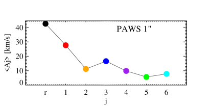
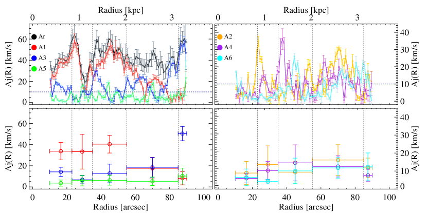
Figure 4: Top plot: Radially averaged mean of the harmonic component amplitudes $A_{j}$ from PAWS 1” residual velocity field. Bottom plot: Non-circular motion amplitudes from harmonic decomposition: radial trend of the odd components and the total power $A_{r}(R)$ (top left) and even components (top right). The horizontal blue dashed straight line indicates twice the channel width of the datacube, i.e. $2\times 5$ km s^-1 = 10 km s^-1. In the bottom row the mean behavior of the odd (left) and even (middle) components in the different M51 environments as defined in Meidt et al. (2013) (dashed vertical lines; see the text for details) are indicated together with the standard deviations of the values. Horizontal error bars represents the widths of the environments.

5.4.2 Even velocity modes: an additional three-armed spiral structure

The higher resolution maps also provide valuable information about other, weaker modes that appear over a more limited radial range than those associated with the dominant two-armed pattern. Compared to lower spatial resolution data, we can sample this type of mode in PAWS data at 1” and 3” with many more resolution elements.

Fig. 4 shows that there is non-negligible power in several of the even harmonic components, over almost the entire PAWS FoV. The $j$=2 exhibits a strong peak of $\sim 35$ km s^-1 at $R\approx 23"$. Between $25"\lesssim R\lesssim 40"$ the $j$=2 term weakens and the power in the $j$=4 term increases, peaking well above our confidence level ($\sim 35$ km s^-1 at $R\approx 37"$). This switch in dominance between $j$=2 and $j$=4 term is most clear in the PAWS 1” velocity field.

Since a perturbation of $m$ order introduces $j=m-1$ and $j=m+1$ terms in the residual velocity field, non-negligible values of $j$=2 and $j$=4 constitute the first kinematic evidence of an $m=3$ wave within $R\sim 45"$ (i.e. $R\sim 1.7$ kpc) in the disk of M51a. According to the transition between these two components, we estimate that the corotation radius of this mode occurs at $R=(30\pm 3)"$ (i.e. $R=1.1\pm 0.1$ kpc).

The PAWS data at 3” show a similar pattern, including a switch in dominance between $j$=2 and $j$=4 term at a similar radial distance as in PAWS 1”. But given the lower resolution, the detection of the $j$=4 in the region between $45"\lesssim R\lesssim 50"$ occurs over only 5 data points, and the signature is also weaker (the maximum is $\sim 25$ km s^-1). Moving to resolution lower than 3”, the behaviors of $j$=2 and $j$=4 terms are gradually smeared out and the switch in dominance between the two modes is no longer obvious.

An $m$=5 potential perturbation could also be responsible for the $j$=4 term. But, in this case we would expect a more substantial $j$=6 term at larger radii than is measured; only few data points of the $j$=6 term have values above our confidence level. We therefore conclude that this scenario is improbable, or is difficult to detect with the present (spatial and spectral) resolution.

Likewise, since the $j$=2 component, which becomes dominant again outside $R$$\sim$2 kpc, is never accompanied by another transition to a $j$=4 mode with significant power at larger radii, we argue that this must describe a genuine lopsidedness arising with an $m$=1 perturbation.

5.4.3 Outer arms

In the region corresponding to the material arms the PAWS FoV has few data points and the decomposition becomes less accurate. Here it is useful to consider the results from the other lower resolution surveys. The total power of the non-circular components $A_{r}(R)$ increases almost monotonically in all harmonic expansions, from 10-20 km s^-1 in the innermost region to $\sim 30$ km s^-1 at 140”. In the HERACLES 13.5” map the $j=3$ remains dominant across the whole FoV, with $\langle A_{3}\rangle\sim 20-30$ km s^-1.

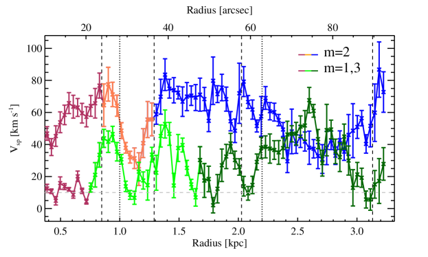
Figure 5: Amplitude of the spiral perturbation from PAWS 1” from the main two-fold spiral arms, three-fold structure and $m=1$ mode. Dark red indicates the radial extent of the bar, orange the molecular ring region, and blue the density-wave spiral arm region as identified from the present-day torque analysis by Meidt et al. (2013). Light green indicates the region of a possible $m=3$ influence, and dark green the non-circular motion induced by the m=1 perturbation. Dotted vertical lines represent the region where Henry et al. (2003) observed a strong signature for a deviation from a pure $m=2$ symmetry. Vertical dashed lines indicate the M51 environments as defined in Meidt et al. (2013) (see the text for details).

5.5 The magnitude of streaming motions

In the previous two sections we used measurements of the power in individual components of the harmonic expansion of the residual line-of-sight velocities observed in M51 to characterize the non-circular motions driven by non-axisymmetric structures. In this section we will give these a physical interpretation, which we will then use to understand the nature of M51’s patterns.

Similarly to Wong et al. (2004), we express the peculiar velocity component $V_{pec}$ in Eq. 7 in terms of the velocities driven in response to a spiral perturbation to the gravitational potential with $m-$fold symmetry, following Canzian & Allen (1997):

$$V_{pec}=V_{sp}\left[\frac{\kappa}{2\Omega}\cos(\theta+\chi)\sin m(\theta-\theta_{sp})+\nu\sin(\theta+\chi)\cos m(\theta-\theta_{sp})\right]\sin i,$$ (7)

Here, $v_{sp}$ is the velocity amplitude that depends on the magnitude of the spiral perturbation, $\theta_{sp}$ is the spiral phase, $\chi$ the spiral arm pitch angle (the angle between the tangent to the arm and a circle with constant radius; by definition $0^{\circ}<\chi<90^{\circ}$) and assuming S-spiral symmetry and trailing spiral arms in the case of M51. The angular frequency $\Omega\equiv(V_{c}/R)^{-1}$, with $R$ the galactic radius in kpc, the pattern speed of the spiral arms is $\Omega_{p}$ and the dimensionless frequency $\nu$ and epicyclic frequency $\kappa$ are defined as

$$\nu\equiv\frac{m(\Omega_{p}-\Omega)}{\kappa},\quad\kappa^{2}\equiv 4\Omega^{2}+R\frac{d\Omega^{2}}{dR}.$$ (8)

As shown by Wong et al. (2004), in the case of a single perturbation with mode $m$, the harmonic decomposition of the peculiar velocities in Eq. 7 yield harmonic coefficients of the form:

$$c_{m\pm 1}=\frac{V_{sp}}{2}\left(\frac{\kappa}{2\Omega}\pm\nu\right)\sin(m\theta_{sp}\pm\chi),$$ (9)

$$s_{m\pm 1}=\frac{V_{sp}}{2}\left(\frac{\kappa}{2\Omega}\pm\nu\right)\cos(m\theta_{sp}\pm\chi).$$ (10)

In the general case of more than one mode $m$, each with its own unique pattern speed $\Omega_{p,m}$, $\chi_{m}$ and $\theta_{sp,m}$, and which each drives its own streaming motions with amplitude $V_{sp,m}$, we can express the amplitudes of any set of harmonic components as

$$A_{m\pm 1}=\sqrt{c_{m\pm 1}^{2}+s_{m\pm 1}^{2}}=\frac{V_{sp,m}}{2}\left(\frac{\kappa}{2\Omega}\pm\nu_{m}\right).$$ (11)

Combining $A_{m-1}$ and $A_{m+1}$ with the definition of the dimensionless frequency $\nu_{m}$ in Eq. 8 we can obtain the following simple parametrization of the amplitude of velocity perturbation:

$$V_{sp,m}=\frac{2\Omega}{\kappa}(A_{m-1}+A_{m+1}).\\$$ (12)

The linear combination of $j$=1 and $j$=3 amplitudes, for instance, provides a measure of the streaming motions driven by an $m$=2 spiral perturbation. In this way, in the presence of more than one mode we can isolate the contributions of individual modes to the total observed non-circular motions. This method for measuring streaming motions also does not need to assume a specific spiral arm pitch angle (observed to vary in M51, e.g. Schinnerer et al. 2013) to perform the decomposition, as required by the technique employed by Meidt et al. (2013).

Similarly, the spiral arm pattern speed $\Omega_{p}$ can be expressed as

$$\Omega_{p,m}=\frac{\kappa}{m}\left(\frac{A_{m+1}-A_{m-1}}{v_{sp,m}}\right)+\Omega.$$ (13)

Note that when $A_{m+1}=A_{m-1}$, $\Omega_{p}=\Omega$. This is a recasting of the prediction by Canzian (1993) that corotation radius (where $\Omega_{p}=\Omega$) is crossed when the $m-1$ switches to an $m+1$ term. However, we emphasize that the pattern speed is likely impossible to estimate reliably in this way, since it depends on $\kappa^{2}$; $\kappa$ itself can be difficult to accurately constrain with observation and is susceptible to uncertainty as it depends on the derivative of $\Omega$ (see Eq. 8). For a recent estimation of the radial variation of the spiral arm pattern speed in M51a through the more reliable and model-independent radial Tremaine-Weinberg (TWR) method, we refer the reader to Meidt et al. (2008).

5.5.1 Streaming motions in M51

In this section we use the results of the harmonic decomposition and our model of M51’s rotation curve to estimate the magnitude of streaming motions (Eq 12) driven in response to the bar, dominant two-armed spiral, the three-armed spiral pattern and/or $m=1$ mode.

We start considering solely the $m=2$ perturbation of the galactic potential. In this case, the quantity of interest is obtainable from the $A_{1}$ and $A_{3}$ as:

$$V_{sp,m=2}=\frac{2\Omega}{\kappa}(A_{1}+A_{3}),$$ (14)

where $\Omega=V_{c}/R$ and $\kappa$ is given by Eq 8.

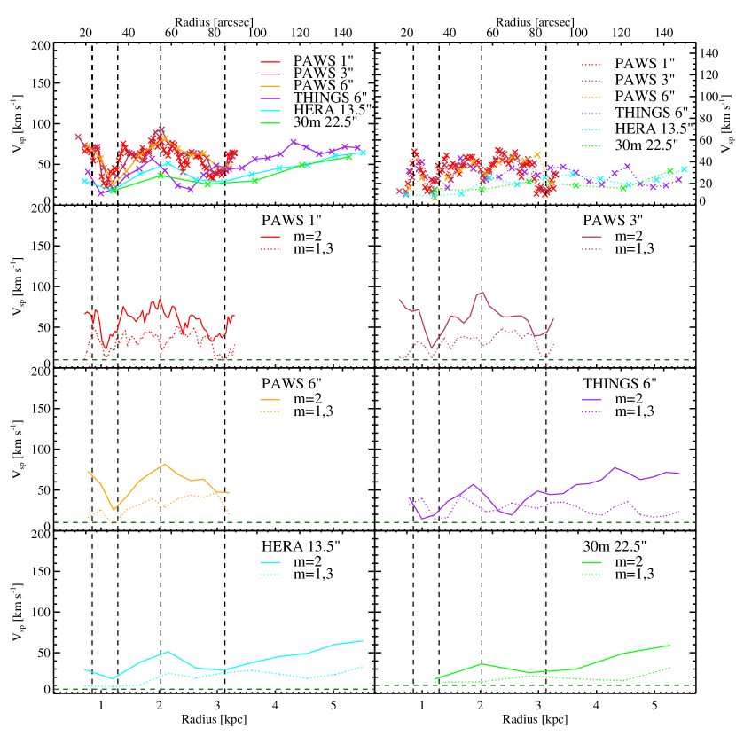
Figure 12: Amplitude of the spiral perturbations from PAWS 1”, PAWS 3”, THINGS 6”, HERACLES 13”, 30m. Solid lines indicate the streaming motion induced by the $m=2$ mode, while the dashed line the streaming motion from the $m=1,3$ mode. The top left panel gives the compact view of the pattern speed derived from the different residual maps given by $m=2$ (left) and $m=1,3$ modes (right).

Fig. 5 and Fig. 12 show the amplitude of velocity of the spiral arm perturbation as derived from Eq. 14 using the harmonic amplitudes from PAWS 1” and lower resolution data residual velocity fields, respectively, as analyzed in Section 5.2. In the nuclear bar region ($R<23"$) streaming motions are $\langle V_{sp,m=2}(R<23")\rangle\approx 60$ km s^-1, in the PAWS 1” data set. Further the streaming motions reach the highest values with a median of $\langle V_{sp,m=2}(35<R<60")\rangle\approx 70$ km s^-1 in PAWS 1” than it decreases again to values around $V_{sp,m=2}(60<R<85")\rangle\approx 50$ km s^-1. However in the lower resolution surveys (i.e. THINGS 6”, HERACLES 13.5” and PAWS single dish 22.5”), $\langle V_{sp,m=2}\rangle$ is always below $\sim 50$ km s^-1 and reaches a value comparable to that recorded in PAWS only in the region of the material arms ($R>85"$). This behavior could be due to beam smearing that reduces the observed peak in streaming motions. As discussed in Section 7, in the case of HI, this could be also due to an intrinsically different response to the spiral perturbation of the potential. In all cases, the spiral perturbation velocity drops in the molecular ring region reaching the minimum of $V_{sp,m=2}\approx 25$ km s^-1 for PAWS 1”, as expected from an analysis of gravitational torques (Meidt et al. 2013).

In Fig. 5 and Fig. 12 we plot also the radial profile of streaming motions that corresponds to the $m$=3 and $m=1$ perturbations, calculated according to:

$$V_{sp,m=1,3}=\frac{2\Omega}{\kappa}(A_{2}+A_{4}),$$ (15)

As described in the previous section, we expect these motions to be related to the $m=3$ wave between $20"<R<45"$ (i.e., $0.8$ kpc $<R<1.7$ kpc), where we observe a peak in the $j$=2 term switching to a peak in a $j=4$ term in the residual velocity field. The start of the $m$=3 mode is taken as the location where the $j$=2 term increases above our 10 km s^-1 confidence threshold, while the end of the $m$=3 mode is set by the decrease in the power of the $j$=4 term. This zone is consistent with the radial range over which the larger deviation from a pure $m=2$ mode was identified ($1$ kpc $<R<2.2$ kpc, Henry et al. 2003). Across this zone, the $m$=3 mode drives streaming motions of $\langle V_{sp,m=3}\rangle\approx 25-30$ km s^-1 on average and reaches a minimum below the confidence limit of 10 km s^-1 in the ring region. (Note that there is little to no power in the zone of the bar where $\langle V_{sp,m=1,3}\rangle\approx 12$ km s^-1, only slightly above our confidence limit). At larger radii, the streaming motions arise from a lopsided ($m$=1) mode (only $j=2$ appears in the harmonic expansion, i.e. $A_{4}\sim$0), with a magnitude of $\langle V_{sp,m=1}\rangle\approx 32$ km s^-1.

6 Discussion: an $m$=3 potential perturbation in M51

In the previous sections we presented kinematic evidence for the existence of an $m$=3 mode, which supplies confirmation of an $m$=3 perturbation to M51s gravitational potential first investigated by Elmegreen et al. (1992). This mode is spatially coincident with the inner part of the dominant two-armed spiral. Presumably, the interference of an $m=3$ wave with the $m=2$ wave enhances the asymmetry in the velocity field (i.e. increasing the deviation in iso-velocity contours from pure circular motion.) This would seem to support the interpretation of Meidt et al. (2008), who consider the likelihood that their inner TWR pattern speed estimate calculated using CO(1-0) as a kinematic tracer reflects a combination of the speed of the $m$=3 mode with that of the dominant two-armed spiral.

This conclusion moreover supports the finding of Henry et al. (2003), who reconsidered the evidence for an $m$=3 perturbation in the old stellar light distribution first studied by Rix & Rieke (1993). They claim that the magnitude of the $m=3$ component in K-band is sufficient to account for the offset between the mirror of one of the two main spiral arms and its counterpart. They also observe patches of molecular gas and star formation in the inter-arm at the location of one of the three arm segments imaged in the K-band.

In the next section we consider the origin of this $m$=3 mode and its density-wave nature, taking into account our analysis of the gas response.

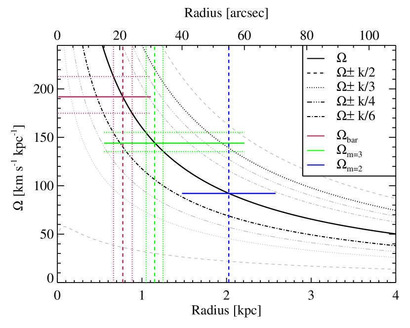
Figure 6: Angular frequency curves derived from the gas-based rotation curve of M51: $\Omega$ (black solid), $\Omega\pm\kappa/2$ (dashed), $\Omega\pm\kappa/3$ (dotted), $\Omega\pm\kappa/4$ (dashed dotted-dotted-dotted) $\Omega\pm\kappa/6$ (dashed-dotted). Angular frequency curves discussed specifically in the text ($\Omega-\kappa/6$, $\Omega+\kappa/3$) are highlighted in black. Pattern speed estimates for the nuclear bar, spiral arms, and m=3 density-wave in M51 are shown in dark red, blue and green, respectively, together with their associated corotation radii and uncertainties (when available).

6.1 Origin, role and nature of the $m=3$ mode

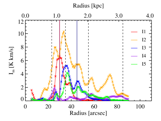
Figure 7: Fourier decomposition of the surface brightness of the PAWS 3” zeroth moment map shown as the power in the Fourier component in K km s^-1. The vertical blue line indicates the boundary between $m=3$ and $m=1$ dominance estimated in Section 5.5.1. The red vertical line represents the $m=3$ corotation at $R\sim 1.1$ kpc. Dashed vertical lines indicates M51’s environments as defined in Meidt et al. (2013).

The PAWS 1” residual velocity field shows a clear kinematic signature of an $m=3$ mode in the central region of M51a. According to Fig. 4 we place its corotation radius at $R_{CR,m=3}\approx(30\pm 3)"$ (i.e. $R_{CR,m=3}\approx 1.1\pm 0.1$ kpc). Together with the angular frequency derived by Meidt et al. (2013), we can define the pattern speed of $\Omega_{m=3}\approx 140\pm 9$ km s^-1 kpc^-1.

Fig. 6 shows that the $m=3$ wave appears to be associated with several interesting resonance overlaps, giving us a picture of very specific interaction between waves. The corotation radius $R_{CR,b}\approx 0.8\pm 0.1$ kpc for the nuclear bar of M51 (Zhang & Buta 2012) overlaps with the inner ultra harmonic resonance (UHR) of the $\Omega_{p,m=3}$ pattern speed (where $\Omega_{p,m=3}$=$\Omega-\kappa/6$). The $m=3$ mode itself extends out to R$\sim 1.7$ kpc (according to where the amplitude of $j=4$ is above our confidence threshold), which is very close to the bar’s outer Lindblad resonance (OLR), the outermost extent of its gravitational influence. This suggests that the bar is a possible driver of the $m=3$ mode. The $m=3$ mode also appears to be connected with the main spiral structure. Indeed, the OLR of the $m$=3 (where $\Omega_{p,m=3}=\Omega+\kappa/3$) overlaps with the corotation radius of the main $m$=2 spiral pattern.

These resonance overlaps may be an instance of non-linear mode coupling. Fig. 7 presents the power in the Fourier decomposition of the PAWS CO(1-0) surface brightness at 3”, revealing power in both the $m=1$ and $m=5$ modes. This is in agreement with predictions by Masset & Tagger (1997) (and studied by Rautiainen & Salo 1999) that coupling between $m=2$ and $m=3$ modes should generate $m=1$ and $m=5$ beat modes. The $m=1$ and $m=5$ modes are particularly strong and confined within the region of influence of the $m=3$ ($R<45"$). Moreover the $m=1$ mode is peaked exactly at the $m=3$ corotation of $R=1.1$ kpc.

This non-linear mode coupling can be interpreted as evidence that the particular $m$=3 structure we find provides the avenue to couple the bar, which we expect appears as a natural instability of the rotating stellar disk, with the dominant two-armed spiral that extends out to larger radii, and which is presumably independently excited by the interaction with M51b. While bars and two-armed spirals are often suggested to naturally couple (in which case the bar is said to ‘drive’ the spiral), in M51 this does not appear to be the case: Fig. 6 shows no compelling direct link between the bar resonances (CR, OLR) and those of the $m$=2 spiral (ILR, UHR, CR). The $m=3$, on the other hand, appear to supply a link between these two structures, presumably in order for energy and angular momentum to be continually transferred radially outward.

These evidences suggest that the $m=3$ mode as a density-wave nature. The transience or longevity of this feature, however, cannot be assessed with our observational data, which provides a snapshot of the current state of M51. We note, though, that multiple spiral structures are generally associated with transient, quickly-evolving spiral arms (e.g. Toomre 1981, Fuchs 2001, D’Onghia et al. 2013). Since we would argue that the coincidence of a three-fold potential perturbation with that of the main $m=2$ pattern definitively excludes a single mode in M51 (like Lowe et al. 1994; Henry et al. 2003) our finding may therefore favor theories of multiple, quickly-evolving density wave spirals.

At larger radii, the residual velocity field harmonic decomposition indicates that the $m=2$ wave may be spatially coincident with an $m=1$ perturbation to the potential. This perturbation is likely responsible for the lopsidedness in K-band images identified, e.g. by Rix & Rieke (1993). To reliably connect the origin of this feature to the interaction with M51b, new high resolution data beyond the PAWS FoV are necessary.

7 Discussion: The Dependence of Kinematic Parameters on Resolution and Gas Tracer

In the previous section we discussed evidence for the existence of an $m=3$ wave in the radial range 0.8 kpc $<$$R$$<$1.7 kpc (i.e. $20<R<45"$) in the center of M51a. The kinematic signature of such a weak, compact mode can be reliably identified only when analyzing the PAWS residual velocity field at a resolution of 1”. At lower spatial resolution (even with equivalent spectral resolution), the presence of such a weak mode becomes less obvious (see Section 5.2). Given that the dominant molecular spiral arm width is around 400 pc (Schinnerer et al. 2013), it is not surprising that high resolution data are needed for an accurate kinematic characterization of the structures traced by molecular gas. Other small scale kinematic features, such as the bright and high-velocity dispersion core of M51a and the spurs on the downstream side of the spiral arms, also only become visible in high resolution velocity fields.

Perhaps more critical to the results of an in-depth kinematic analysis than resolution considerations is the nature and distribution of the kinematic tracer. Indeed, HI emission appears naturally more smooth at all spatial scales (Leroy et al. 2013), which may make it less sensitive to small-scale potential perturbations than the highly clumpy medium traced by CO radiation.

For this reason, to correctly characterize spiral arm gas kinematics a gas phase tracer that is strongly affected by the mid-plane galactic potential and interferometric observations that are able to resolve them are preferred. In the following we illustrate how the nature of the tracer and the observing strategy for a given dataset impacts the interpretation of the kinematic properties measured for spiral galaxies like M51.

7.1 CO versus HI kinematics

Recent studies have shown that the 3-dimensional distributions of the atomic and molecular gas in M51 are not identical (e.g. Schinnerer et al. 2013, Pety et al. 2013). Therefore we expect to find differences in their kinematics as well. The CO line emission is closely associated with the spiral arms tracing the density enhancement in the old stellar population, while the emission from the atomic gas is fairly smooth and its brigthness distribution relative to the spiral arm suggests that it may be produced via the photodissociation of H₂. (e.g. Smith et al. 2000, Schinnerer et al. 2013, Louie et al. 2013). Moreover, the velocity dispersion observed in the CO-bright compact component emission is very different from the HI line emission, $\sim 5$ km s^-1 (Pety et al. 2013) versus $\sim 15$ km s^-1 (e.g. Tamburro et al. 2009, Caldú-Primo et al. 2013), respectively. According to Koyama & Ostriker (2009) equation 2, this implies that the CO bright emission arises from a thinner disk than the HI radiation.

The different distribution of the molecular and atomic gas is also strongly reflected in their velocity fields from which all kinematic information is derived. As noted in Section 3, the PAWS CO velocity field tapered to 6” still shows several of prominent non-circular motion features that are clearly visible at 1” resolution while these features are basically absent in the THINGS HI cube at the same 6” resolution. (R2a) The first direct consequence is that rotation curves derived from CO and HI velocity fields are very different (Fig 8, top). Rotation curves from PAWS CO datasets show strong bumps and wiggles at both 1” and 6” resolution. These features are mostly absent in the THINGS rotation curve, which is much smoother than the rotation curve obtained using the CO data. In the latter, the presence of wiggles presumably reflects a contribution from azimuthal non-circular streaming motions in regions where the spiral arms dominate the tilted-ring fit compared to the relatively streaming-free inter-arm region.

For similar reasons, the residual velocity field from PAWS shows clear signatures of non-circular motion that are not present in the THINGS residual velocity field at the same resolution, pixel size and FoV (Fig. 9, top left). Since those velocity fields are central to study spiral perturbations we illustrate their differences more quantitatively using pixel-by-pixel diagrams (Fig. 9, top right). The pixel-by-pixel comparison reveals a large scatter between values measured in the two residual velocity fields . Such differences naturally influence the measurement of the velocity associated with the potential perturbation $V_{sp}$ (Fig 8, bottom), which depends on the amplitude of (non-circular) harmonic components in the residual velocity field (see Eq. 12). Whereas the magnitudes of the streaming motions derived using the PAWS 1” and 6” data are comparable, the value derived from the THINGS 6” data is on average $\ sim35$ km s^-1 lower than $V_{sp}$ obtained from PAWS 6” in the region between $R\sim 60-80"$.

Our conclusion is that due to the different spatial distributions of the atomic and molecular gas (both in and above the disk plane), CO and HI emission trace the galactic potential differently. Since the CO emission has a radial and vertical distribution that correlates very well with the location of the stellar spiral potential in M51, it is an optimal tracer for detailed kinematic characterization of the mid-plane potential. Meanwhile, the atomic gas sits further away from the mid-plane and offset from the spiral arms so that it experiences a slightly different (and weaker) spiral perturbation. As a result, CO is a better tracer of streaming motions, but HI yields better constraints on the bulk motion of the galaxy (i.e. the rotation curve and other global kinematic parameters).

7.2 Hybrid versus single-dish data

Interferometers filter out low spatial frequencies, i.e., spatially extended emission. For this reason, the type of observational data that is used will affect the way a given gas phase observation traces motions driven in response to the gravitational potential. Single dish observations are likely to be more sensitive to fluffy emission from a more vertically extended component, as was recently discovered for the 30m and hybrid 30m+PdBI observations of M51 by Pety et al. (2013). As discussed at the end of the previous section, this may prevent single-dish observations from revealing the same pattern of streaming motions that are evident even in the hybrid data after degrading its resolution.

The middle row of Figure 9 shows this in a little more detail, comparing the PAWS and HERACLES residual velocity fields smoothed to the same 13.5” resolution. Even at 13.5”, the PAWS residual velocity field still exhibits the typical signatures of bar and spiral arm streaming motions. But these departures from circular motion are less clearly visible in the HERACLES residual velocity field. The pixel-by-pixel diagram confirms that the two maps are not the same, as large scatter is present.

The line-width measured from HERACLES IRAM 30m observations is significantly larger than measured from PAWS at 1”. Some part of this could be due to unresolved bulk motions. Caldú-Primo et al. (2013) measured similar velocity dispersions for CO from HERACLES and HI from THINGS observations in a sample of 12 galaxies, which would imply that the two phases have similar vertical distributions. They find, for M51 in particular, $\sigma_{HI}\sim\sigma_{CO}\approx$ 15 km s^-1. This value is comparable to the velocity dispersion of the extended CO component measured by Pety et al. (2013) for M51, rather than the compact CO emission that dominates the PAWS second moment map (see Pety et al. 2013). This suggests that the single-dish data are dominated by the vertically extended gas than the hybrid data, which mainly traces gas that is more confined to the disk mid-plane, and thus more influenced by the gravitational potential.

We have considered whether the difference between hybrid PAWS and HERACLES at 13.5” resolution arises from the fact that the two observations sample two different tracers of the molecular gas: while PAWS traces ¹²CO(1-0) emission, HERACLES traces ¹²CO(2-1). In the last row of Fig 8, we compare the residual velocity fields from the PAWS single-dish data with HERACLES observations, smoothed to the same 22.5” resolution. Since both observations have been obtained with the same instrument (IRAM 30m antenna), instrumental effects should be negligible. These maps show only small differences, and the scatter in the pixel-by-pixel comparison is very low. We conclude that, from a kinematic point of view, single-dish observations of ¹²CO(1-0) and ¹²CO(2-1) provide similar results.

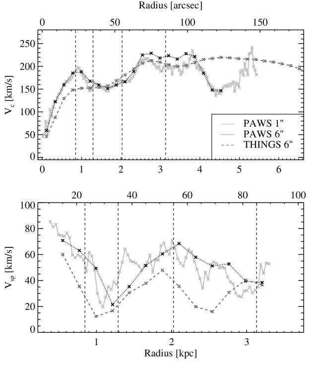
Figure 8: Rotation curves (top) and amplitude of the two-armed spiral arm perturbation (bottom) derived from PAWS 1”, PAWS 6” and THINGS 6” derived with the GIPSY task ROTCUR and the method described in Section 5, respectively. Vertical dashed lines represent M51’s environments as defined in Meidt et al. (2013). The dip at $R\sim 100-150"$ in the PAWS 1” rotation curve is probably caused by the low inter-arm sampling due to the rectangular shape of the PAWS FoV that leads the fit to favor the spiral arms.

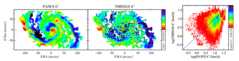
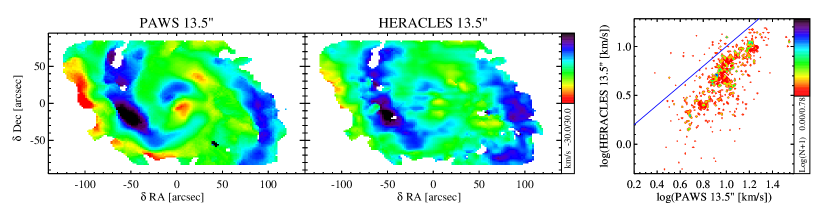
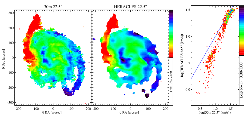
Figure 9: Comparison between PAWS 6” and THINGS 6” (top), PAWS 6” smoothed to 13.5” and HERACLES, PAWS single dish and HERACLES smoothed to 22.5” (bottom) residual velocity fields, on the same pixel size and FoV. The operations are performed using the MIRIAD tasks CONVOL and REGRID on the datacubes. Residual velocity fields are obtained using the procedure described in Section 5.1. The right panels show the pixel-by-pixel comparisons of the residual velocity fields in value of the pixels. Number densities of the points are in logarithmic scale. Blue lines indicate the 1:1 relation.

8 Summary

In this paper we performed a detailed kinematic analysis of the inner disk of M51 with the aim of characterizing and quantifying the non-circular motions driven in response to the bar and spiral patterns present in the disk. Our primary focus is the view of gas motions presented by the high resolution PAWS 1” ¹²CO(1-0) data set, in addition we support the interpretation of our findings with other lower resolution datasets (PAWS 3” and 6” ¹²CO(1-0), THINGS 6” HI, HERACLES 13.5” ¹²CO(2-1) and PAWS single dish 22.5” ¹²CO(1-0)). Our main results are summarized as follows:

• By applying a tilted ring analysis to the different velocity fields, we obtained updated estimates of projection parameters of M51, namely position angle $PA=(173\pm 3)^{\circ}$ and inclination $i=(22\pm 5)^{\circ}$. We use these to fit for the circular velocity in each of the data sets.

• We perform a harmonic decomposition of the residual velocity fields in order to identify, separate and inspect the contributions of the different modes to the global pattern of non-circular motions in the galaxy. The residual velocity field of M51 is complex, but shows the clear signature of arm-driven inflow (especially along the southern arm) and the butterfly pattern of the inner bar.

  • The dominant $m=2$ mode is characterized by a corotation radius at $R_{CR,m=2}\approx 2.4$ kpc ($R_{CR,m=2}\approx 60"$), consistent with location of the corotation of the two-armed spiral indicated by the gravitational torque analysis of Meidt et al. (2013).

  • Coincident with this mode, we find the first unequivocal evidence for an $m=3$ mode in the inner disk of M51, extending out to $R\approx 1.7$ kpc ($R\approx 45"$). The kinematic signature of this mode allows us to estimate the location of its corotation radius $R_{CR,m=3}\approx 1.1\pm 0.1$ kpc ($R_{CR,m=3}\approx 30\pm 3"$).

  • Inspection of the angular frequency curves suggests that the $m=3$ mode may be coupled to, and stimulated by, the nuclear bar. Evidence for the dynamical coupling between the three-armed spiral and the main two-fold pattern at the overlap of their resonances is suggested by the appearance of $m=1$ and $m=5$ components in the CO surface brightness around the overlap. This supports the density-wave nature of the three-armed perturbation to the potential traced by the gas motions.

• Combining the amplitudes of the individual harmonic components, we obtained a simple expression for the streaming motion amplitude of the main modes in M51.

  The streaming motions from the main $m$=2 mode range from $\langle V_{sp,m=2}\rangle\approx 70$ km s^-1 in spiral arm region devoid of star formation to $\langle V_{sp,m=2}\rangle\approx 50$ km s^-1 in the outer density-wave spiral arms, and exhibit a minimum $\langle V_{sp,m=2}\rangle\approx 25$ km s^-1 in the molecular ring region.

  The streaming motion from the secondary modes ($m=1,3$) are $V_{sp,m=3}\lesssim 30$ km s^-1 in the region influenced by the $m=3$ mode and $\langle V_{sp,m=1}\rangle\approx 32$ km s^-1 in the region dominated by the $m=1$ mode, but no higher than $V_{sp,m=1,3}\approx 20$ km s^-1 in the bar region.

• The joint analysis of velocity fields obtained from different gas tracers at different resolutions suggests the following guidelines for defining the most appropriate observing strategy to meet a given scientific goal:

  • high resolution CO surveys are particularly well-suited for detailed studies of non-circular motion features, while low resolution observations are equally as important for defining the bulk motion of the galaxies (i.e. rotation curves). In the presence of modes that extend over only a limited radial range, as in M51, and when complex, overlapping structure exists generally, high resolution is key to identifying and characterizing such modes.

  • CO and HI can supply independent views of the gravitational potential, as suggested by different natures of the two gas phases; while the atomic gas in M51 has a smooth distribution, is located mostly downstream of the spiral arms and in a thicker disk, the molecular gas is more compact, organized in a thinner disk and mostly confined to the spiral arms. Given the differences in velocity dispersion and morphology, we conclude that CO is optimal for tracing spiral arm streaming motions and, in general, for studying the galactic potential, while HI is more suitable for obtaining the bulk motion and the projection parameters of the galaxies.

Appendix A Low-resolution velocity field harmonic decomposition and amplitude of spiral perturbations

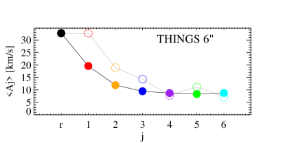
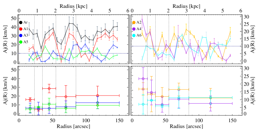
Figure 10: Top plot: Radially averaged mean of the harmonic component amplitudes $A_{j}$ from THINGS 6” residual velocity field. Open dots indicate the measurements restricted on the PAWS FoV. Bottom plot: Non-circular motion amplitudes from harmonic decomposition: radial trend of the odd components and the total power $A_{r}(R)$ (top left) and even components (top right). The horizontal blue dashed straight line indicates twice the channel width of the datacube, i.e. $2\times 5$ km s^-1 = 10 km s^-1. In the bottom row the mean behavior of the odd (left) and even (middle) components in the different M51 environments as defined in Meidt et al. (2013) (dashed vertical lines; see the text for details) are indicated together with the standard deviations of the values. Horizontal error bars represents the widths of the environments.

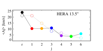
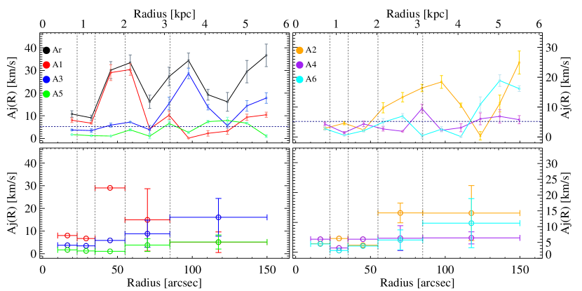
Figure 11: Top plot: Top plot: Radially averaged mean of the harmonic component amplitudes $A_{j}$ from HERACLES 13.5” residual velocity field. Open dots indicate the measurements restricted on the PAWS FoV. Bottom plot: Non-circular motion amplitudes from harmonic decomposition: radial trend of the odd components and the total power $A_{r}(R)$ (top left) and even components (top right). The horizontal blue dashed straight line indicates twice the channel width of the datacube, i.e. $2\times 2.6$ km s^-1 = 5.2 km s^-1. In the bottom row the mean behavior of the odd (left) and even (middle) components in the different M51 environments as defined in Meidt et al. (2013) (dashed vertical lines; see the text for details) are indicated together with the standard deviations of the values. Horizontal error bars represents the widths of the environments.

References

- Bertin & Lin (1996) Bertin, G., & Lin, C. C. 1996, Spiral structure in galaxies a density wave theory
- Bertin et al. (1989a) Bertin, G., Lin, C. C., Lowe, S. A., & Thurstans, R. P. 1989a, ApJ, 338, 78
- Bertin et al. (1989b) —. 1989b, ApJ, 338, 104
- Bigiel et al. (2008) Bigiel, F., Leroy, A., Walter, F., et al. 2008, AJ, 136, 2846
- Caldú-Primo et al. (2013) Caldú-Primo, A., Schruba, A., Walter, F., et al. 2013, AJ, 146, 150
- Canzian (1993) Canzian, B. 1993, ApJ, 414, 487
- Canzian & Allen (1997) Canzian, B., & Allen, R. J. 1997, ApJ, 479, 723
- Ciardullo et al. (2002) Ciardullo, R., Feldmeier, J. J., Jacoby, G. H., et al. 2002, ApJ, 577, 31
- de Blok et al. (2008) de Blok, W. J. G., Walter, F., Brinks, E., et al. 2008, AJ, 136, 2648
- Dobbs et al. (2010) Dobbs, C. L., Theis, C., Pringle, J. E., & Bate, M. R. 2010, MNRAS, 403, 625
- D’Onghia et al. (2013) D’Onghia, E., Vogelsberger, M., & Hernquist, L. 2013, ApJ, 766, 34
- Dressel & Condon (1976) Dressel, L. L., & Condon, J. J. 1976, ApJS, 31, 187
- Elmegreen et al. (1992) Elmegreen, B. G., Elmegreen, D. M., & Montenegro, L. 1992, ApJS, 79, 37
- Fathi et al. (2005) Fathi, K., van de Ven, G., Peletier, R. F., et al. 2005, MNRAS, 364, 773
- Ford et al. (1985) Ford, H. C., Crane, P. C., Jacoby, G. H., Lawrie, D. G., & van der Hulst, J. M. 1985, ApJ, 293, 132
- Fuchs (2001) Fuchs, B. 2001, A&A, 368, 107
- Goad et al. (1979) Goad, J. W., de Veny, J. B., & Goad, L. E. 1979, ApJS, 39, 439
- Hagiwara et al. (2001) Hagiwara, Y., Henkel, C., Menten, K. M., & Nakai, N. 2001, ApJ, 560, L37
- Hagiwara (2007) Hagiwara, Y. 2007, AJ, 133, 1176
- Henry et al. (2003) Henry, A. L., Quillen, A. C., & Gutermuth, R. 2003, AJ, 126, 2831
- Koyama & Ostriker (2009) Koyama, H., & Ostriker, E. C. 2009, ApJ, 693, 1346
- Kuno & Nakai (1997) Kuno, N., & Nakai, N. 1997, PASJ, 49, 279
- Leroy et al. (2009) Leroy, A. K., Walter, F., Bigiel, F., et al. 2009, AJ, 137, 4670
- Leroy et al. (2013) Leroy, A. K., Lee, C., Schruba, A., et al. 2013, ApJ, 769, L12
- Leroy et al. (2013) Leroy, A. K., Walter, F., Sandstrom, K., et al. 2013, AJ, 146, 19
- Lindblad (1963) Lindblad, B. 1963, Stockholms Observatoriums Annaler, 22, 5
- Lin & Shu (1964) Lin, C. C., & Shu, F. H. 1964, ApJ, 140, 646
- Louie et al. (2013) Louie, M., Koda, J., & Egusa, F. 2013, ApJ, 763, 94
- Lowe et al. (1994) Lowe, S. A., Roberts, W. W., Yang, J., Bertin, G., & Lin, C. C. 1994, ApJ, 427, 184
- Maddox et al. (2007) Maddox, L. A., Cowan, J. J., Kilgard, R. E., Schinnerer, E., & Stockdale, C. J. 2007, AJ, 133, 2559
- Masset & Tagger (1997) Masset, F., & Tagger, M. 1997, A&A, 322, 442
- Matsushita et al. (2007) Matsushita, S., Muller, S., & Lim, J. 2007, A&A, 468, L49
- Meidt et al. (2008) Meidt, S. E., Rand, R. J., Merrifield, M. R., Shetty, R., & Vogel, S. N. 2008, ApJ, 688, 224
- Meidt et al. (2013) Meidt, S. E., Schinnerer, E., Garcia-Burillo, S., et al. 2013, arXiv:1304.7910
- Minchev et al. (2012) Minchev, I., Famaey, B., Quillen, A. C., et al. 2012, A&A, 548, A126
- Pety et al. (2013) Pety, J., Schinnerer, E., Leroy, A. K., et al. 2013, arXiv:1304.1396
- Rautiainen & Salo (1999) Rautiainen, P., & Salo, H. 1999, A&A, 348, 737
- Regan et al. (2001) Regan, M. W., Thornley, M. D., Helfer, T. T., et al. 2001, ApJ, 561, 218
- Rix & Rieke (1993) Rix, H.-W., & Rieke, M. J. 1993, ApJ, 418, 123
- Roberts & Stewart (1987) Roberts, W. W., Jr., & Stewart, G. R. 1987, ApJ, 314, 10
- Rogstad et al. (1974) Rogstad, D. H., Lockhart, I. A., & Wright, M. C. H. 1974, ApJ, 193, 309
- Salo & Laurikainen (2000) Salo, H., & Laurikainen, E. 2000, MNRAS, 319, 377
- Schoenmakers et al. (1997) Schoenmakers, R. H. M., Franx, M., & de Zeeuw, P. T. 1997, MNRAS, 292, 349
- Scoville et al. (1998) Scoville, N. Z., Yun, M. S., Armus, L., & Ford, H. 1998, ApJ, 493, L63
- Schinnerer et al. (2013) Schinnerer, E., Meidt, S. E., Pety, J., et al. 2013, arXiv:1304.1801
- Sellwood & Binney (2002) Sellwood, J. A., & Binney, J. J. 2002, MNRAS, 336, 785
- Shetty et al. (2007) Shetty, R., Vogel, S. N., Ostriker, E. C., & Teuben, P. J. 2007, ApJ, 665, 1138
- Schruba et al. (2011) Schruba, A., Leroy, A. K., Walter, F., et al. 2011, AJ, 142, 37
- Schuster et al. (2004) Schuster, K.-F., Boucher, C., Brunswig, W., et al. 2004, A&A, 423, 1171
- Smith et al. (2000) Smith, D. A., Allen, R. J., Bohlin, R. C., Nicholson, N., & Stecher, T. P. 2000, ApJ, 538, 608
- Tamburro et al. (2009) Tamburro, D., Rix, H.-W., Leroy, A. K., et al. 2009, AJ, 137, 4424
- Toomre & Toomre (1972) Toomre, A., & Toomre, J. 1972, BAAS, 4, 214
- Toomre (1981) Toomre, A. 1981, Structure and Evolution of Normal Galaxies, 111
- Trachternach et al. (2008) Trachternach, C., de Blok, W. J. G., Walter, F., Brinks, E., & Kennicutt, R. C., Jr. 2008, AJ, 136, 2720
- Tully (1974) Tully, R. B. 1974, ApJS, 27, 437
- Tully (1974) Tully, R. B. 1974, ApJS, 27, 449
- Turner & Ho (1994) Turner, J. L., & Ho, P. T. P. 1994, ApJ, 421, 122
- van der Kruit & Shostak (1982) van der Kruit, P. C., & Shostak, G. S. 1982, A&A, 105, 351
- van de Ven & Fathi (2010) van de Ven, G., & Fathi, K. 2010, ApJ, 723, 767
- Vogel et al. (1993) Vogel, S. N., Rand, R. J., Gruendl, R. A., & Teuben, P. J. 1993, PASP, 105, 666
- Walter et al. (2008) Walter, F., Brinks, E., de Blok, W. J. G., et al. 2008, AJ, 136, 2563
- Wong et al. (2004) Wong, T., Blitz, L., & Bosma, A. 2004, ApJ, 605, 183
- Zaritsky et al. (1993) Zaritsky, D., Rix, H.-W., & Rieke, M. 1993, Nature, 364, 313
- Zhang & Buta (2012) Zhang, X., & Buta, R. J. 2012, arXiv:1203.5334