Landau-Zener transitions mediated by an environment: population transfer and energy dissipation

Abstract

We study Landau-Zener transitions between two states with the addition of a shared discretized continuum. The continuum allows for population decay from the initial state as well as indirect transitions between the two states. The probability of nonadiabatic transition in this multichannel model preserves the standard Landau-Zener functional form except for a shift in the usual exponential factor, reflecting population transfer into the continuum. We provide an intuitive explanation for this behavior assuming independent individual transitions between pairs of states. In contrast, the probability of survival in the ground state at long time shows a novel, non-monotonic, functional form, with an oscillatory behavior in the sweep rate at low sweep rate values. We contrast the behavior of this open-multistate model to other generalized Landau-Zener models incorporating an environment: the stochastic Landau-Zener model and the dissipative case, where energy dissipation and thermal excitations affect the adiabatic region. Finally, we present evidence that the continuum of states may act to shield the two-state Landau-Zener transition probability from the effect of noise.

I Introduction

Systems that may be modeled by avoided level crossings are ubiquitous in nature and in artificial mesoscopic systems. In 1932, Zener Zen , Landau Land , Stueckelberg Stueck , and Majorana Maj separately derived an expression describing the probability of nonadiabatic transitions at avoided level crossings, based on semi-classical modeling. The result, typically referred to as the “Landau-Zener” (LZ) formula, has been applied to describe transition probabilities in the context of chemical reactions Reaction , production of cold molecules ColdRev , quantum electrodynamic circuits QED1 ; QED2 , spin-flip in nanomagnets nanmag , Bose-Einstein condensates in optical lattices BEcond , doublon-hole production in a Mott insulator Oka , directed quantum transport in bipartite lattices bipartite , and adiabatic computing QAdi ; AdComp . Furthermore, the LZ model has been used to design the Landau-Zener-Stueckelberg spectroscopy technique LZS .

The original Landau-Zener problem is restricted to two coupled diabatic levels with an energy gap that is linearly modified in time at a constant rate. Given a certain initial state, the ground diabatic state, the quantities of interest are the population probabilities for both the ground and the excited diabatic states at infinitely long time, far from the crossing region. This minimal LZ situation has been revisited many times and extended to a broader class of systems; in particular, the multistate Landau-Zener problem, a representative of time-dependent Hamiltonians, has been studied analytically and numerically in Refs. DemOsh ; Brundobler ; Nogo ; Sym ; Sinitsyn ; BT ; NBT ; GBT1 ; GBT2 ; SpinBath ; Akulin ; Moyer ; Band . In such models it has generally been argued that the probability to remain in the initial diabatic state (in other words, to make a nonadiabatic transition) follows a semiclassical behavior: It decreases exponentially with the number of avoided crossings $N$, $P_{na}\sim e^{-\beta N}$, where $\beta$ characterizes the transition probability at an individual crossing. This form is valid as long as the energy of the initial state follows a linear dependence in time Sinitsyn .

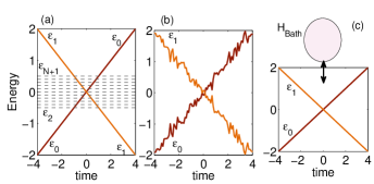
Figure 1: Schemes of the different models studied in this work. (a) Open-multistate Landau-Zener problem. The diabatic energies of the original LZ problem are presented by full diagonal lines. The dashed lines represent stationary states of a dense continuum. Parameters correspond to the sweep velocity $\alpha=1$, tunneling element $\Delta=0.1$ and the band cutoff $D=0.5$. (b) Stochastic-Markov LZ model. The energy difference between the diabatic states fluctuates around the original LZ value. (c) Dissipative LZ model with the diabats coupled to a (finite-temperature) harmonic heat bath.

However, in physical situations a quantum system is never truly isolated from its environment, which can have the effect of inducing phase decoherence, population relaxation, energy dissipation, and bath-induced transitions. This problem has been studied extensively in different regimes of sweeping speed, temperature, and system-environment coupling strength, using an array of perturbative approaches; see for example the early study of Tsukada Tsukada and other comprehensive works Gefen ; Ao ; Stern ; KayanumaPRB ; Sun ; spin ; Ziman ; Band . While the transition probability can be obtained exactly-analytically when the diabats are coupled to a zero-temperature bath HanggiT0 , at nonzero temperatures, numerically-exact simulations have been reported in Refs. Thorwart ; LeHur , revealing a rich dynamics. Specifically, it has been shown that at a nonzero temperature the (harmonic) heat bath is responsible for transition probabilities that are non-monotonic in the sweep velocity, the result of a nontrivial competition between the driving (sweep) and bath-induced excitation and relaxation processes Thorwart .

Our primary objective in this paper is to study the nonadiabatic transition probabilities of the open-multistate LZ model, consisting of two driven states (as in the original LZ model) coupled to a finite-band discretized continuum consisting of stationary states. The avoided crossing between the driven states occurs directly at the center of the finite band, as shown in Fig. 1(a). The continuum allows for indirect transitions between the two main diabats, mediated by population transfer to the continuum. This setup can be used to model, for example, multichannel reactions with intermediates and competing products Tully1 ; Tully2 . In the context of mesoscopic devices, the model can serve to describe all-electrical population transfer processes between spatially separated quantum dots coupled indirectly via a chain of intermediating dots CTAP ; Kohler or through a central metal Gurvitz . One could also consider quantum memory preservation in a spin quit interacting with its environment, or a similar system. Here environmental processes may induce in an unintended spin flip, resulting in memory loss. Understanding these processes should make it possible to better control them.

We note that the LZ model with the discretized continuum, as depicted in Fig. 1(a), is an example of a multistate LZ model. Using numerical simulations we show below that while the nonadiabatic transition probability $P_{na}$ follows an exponential decaying form (similar to other multistate LZ models appearing in the literature as discussed above) the ground state survival probability in our model displays nontrivial and non-monotonic features, revealing indirect pathways between the two diabats. We explain these signatures and further contrast them to the fingerprints of energy dissipation and thermal excitation processes. We do so by constructing several elementary models as shown in Fig. 1: (a) The open-multistate LZ model, as discussed above, with the two driven states coupled to a finite-band discrete stationary continuum. (b) The stochastic (infinite temperature) model, where the isolated LZ Hamiltonian suffers from noise, responsible for energy fluctuations Kayanuma-stoA . (c) The dissipative finite temperature LZ many-body model, where the two driven states are bilinearly coupled to a harmonic heat bath.

The paper is organized as follows. In Sec. II we describe variants of the LZ model that allow us to pinpoint how the original LZ problem is modified by its coupling to a stationary continuum or a heat bath. Numerical results are included in Sec. III along with detailed analysis. In Sec. IV we discuss and conclude our observations. For simplicity, we set $\hbar=1$ and $k_{B}=1$ throughout this paper.

II Models

II.1 Isolated Landau-Zener model

The original LZ model includes two diabatic states $|0\rangle$ and $|1\rangle$ with a fixed tunneling matrix element $\Delta$. The energies of these states are modified linearly in time, $\epsilon_{0}=\alpha t/2$, $\epsilon_{1}=-\alpha t/2$ at a sweep rate $\alpha$ (dimension Energy²),

$$H_{LZ}^{iso}(t) = \epsilon_{0}(t)|\,{0}\,\rangle\langle\,{0}\,|+\epsilon_{1}(t)|\,{1}\,\rangle\langle\,{1}\,|$$ (1)

$$+ \Delta|\,{0}\,\rangle\langle\,{1}\,|+{\Delta}|\,{1}\,\rangle\langle\,{0}\,|.$$

Since the two states are isolated (iso) from an environment, we refer to this as the “closed LZ model.” At large negative time, before approaching the avoided crossing, the system is prepared in the ground state corresponding to $|\,{0}\,\rangle$. We define the “survival probability” $P_{s}$ as the probability for the system to end up at long time in the ground state (thus cross diabats). Meanwhile $P_{na}$ describes the probability to stay on the same state $|0\rangle$, thus to make a nonadiabatic transition. In terms of the time evolution operator $U_{\infty}=\mathcal{T}\exp[-i\int_{-\infty}^{\infty}H_{LZ}^{iso}(\tau)d\tau]$, where $\mathcal{T}$ is the time ordering operator, these quantities are defined as

$$P_{s} \equiv P_{0\rightarrow 1}=|\langle 1|U_{\infty}|0\rangle|^{2},$$

$$P_{na} \equiv P_{0\rightarrow 0}\equiv|\langle 0|U_{\infty}|0\rangle|^{2}.$$ (2)

These probabilities add to unity in the closed LZ model. The nonadiabatic transition probability is given by

$$P_{na}^{iso}=\exp(-2\pi\Delta^{2}/\alpha).$$ (3)

This exact expression can be derived based on the solution of the Weber equation Zen , or by two different methods Dykhne ; Wittig that rely on a direct contour integration in the complex $t$-plane.

II.2 Open-multistate Landau-Zener model

We extend the two-state Hamiltonian (1) and describe the “open-multistate LZ model”, including a band of parallel-stationary levels, to account for population relaxation and competing pathways. The multistate model includes the original diabats, which are considered as the system of primary interest (e.g., principal reactant and product, the two states of a qubit, or the states of two separated quantum dots), and a discretized continuum with $N-1$ levels numbered from $2,3,...,N+1$. The corresponding Hamiltonian is given by

$$H_{LZ}^{open}(t) = H_{LZ}^{iso}(t)+\sum\limits_{j=2}^{N+1}{\epsilon_{j}|\,{j}\,\rangle\langle\,{j}\,|}+\sum\limits_{j=2}^{n+1}{v_{0,j}|\,{0}\,\rangle\langle\,{j}\,|}$$ (4)

$$+ \sum\limits_{j=2}^{N+1}{v_{1,j}|\,{1}\,\rangle\langle\,{j}\,|}+h.c.$$

The continuum energies extend from $-D$ to $D$, and each of the continuum states $|j\rangle$ couples to both diabatic levels $n=0,1$ through the tunneling element $v_{n,j}$. We assume a constant density of states $\rho=(N-1)/2D$, and define the hybridization energy as

$$\Gamma_{n}(\epsilon)=2\pi\sum_{j}|v_{n,j}|^{2}\delta(\epsilon-\epsilon_{j});\,\,\,\,\,\,n=0,1.$$ (5)

Since we are considering a discretized continuum, the model (4) can be viewed from different perspectives. In the first picture the $N-1$ additional states are introduced to capture a true continuum to which the diabats are coupled. While we focus here on a shared continuum, facilitating indirect transfer between the levels, in the related ”lossy LZ model” the population of the diabats relax to separate reservoirs. This situations has been investigated analytically in several works by introducing an imaginary term to the diagonal elements of the Hamiltonian, see for example Refs. Akulin ; Moyer ; Band . This model then becomes complementary to the dissipative LZ case where energy relaxation is included KayanumaPRB ; HanggiT0 ; Thorwart . The second interpretation of the model is simply as a multistate LZ model, when the states are allowed to become sufficiently dense DemOsh ; Brundobler ; Nogo ; Sym ; Sinitsyn ; BT ; NBT ; GBT1 ; GBT2 . Indeed several of the multistate LZ setups may be obtained as special cases of the present model: If we set $\Delta=0$, then we obtain a simplified version of the bow-tie model BT ; NBT (generalized bow-tie model GBT1 ; GBT2 ) when we further choose $N=1$ ($N=2$). Alternately, if we nullify both $\Delta$ and $\Gamma_{1}$ (equivalent to removing $|\,{1}\,\rangle$ from the model entirely) we arrive at the Demkov-Osherov model DemOsh . From a different direction, in the absence of driving ($\alpha=0$) the model can describe population transfer between two distant quantum wells that are separated by an intermediate level CTAP ; Kohler or by a common reservoir Gurvitz . In the case of a central reservoir it has been shown that while the system possesses a continuum spectrum, it includes bound states in the continuum responsible for quantum effects such as the formation of an entangled state in the spatially separated wells Gurvitz .

The nonadiabatic transition probability is defined here in a similar fashion to the closed case (2). We evaluate it numerically by propagating the initial state $|\Psi(t=-\infty)\rangle=|0\rangle$ through a sequence of short time-evolution operators

$$|\Psi(t+\delta t)\rangle=e^{-iH_{LZ}^{open}(t)\delta t}|\Psi(t)\rangle.$$ (6)

Numerical parameters are determined following several considerations. First, we recall that transitions in the closed system are characterized by the time scale $\tau_{tr}\sim\frac{2\pi}{\Delta}$. In the open-system model two additional relevant timescales are identified as $\frac{2\pi}{\Gamma_{0}}$ and $\frac{2\pi}{\Gamma_{1}}$. As such, the simulation timestep $\delta t$ must satisfy

$$1/\delta t\gg max\{\Delta,\Gamma_{0},\Gamma_{1}\}.$$ (7)

Another consideration involves the initial $t_{-}$ and final $t_{+}$ simulation times. These times should be taken long enough so that the initial state is prepared (and the final state is reached) far away from the crossing point,

$$|t_{\pm}|\gg max\left\{\frac{\Delta}{\alpha},\frac{\Gamma_{0}+D}{\alpha},\frac{\Gamma_{1}+D}{\alpha}\right\}.$$ (8)

Our main objective here is to understand the dynamics under the Hamiltonian (4) by identifying signatures of population relaxation and indirect transfer in the LZ transition rate. To achieve this goal we now present other related-complementary models, which allow for different effects, energy dissipation and thermal excitation.

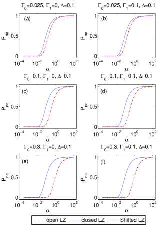
Figure 2: Nonadiabatic transition probabilities in the open-multistate LZ model. Presented are the LZ formula from Eq. (3) (full line), the probability obtained from simulations with a continuum of 41 states and $D=1/2$ (dashed), and $P_{na}^{shift}$ from Eq. (14) (dotted). The open-multistate model is studied for three coupling strength values of $|\,{0}\,\rangle$ and $|\,{1}\,\rangle$ to the continuum, denoted by $\Gamma_{0}$ and $\Gamma_{1}$ respectively.

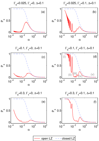
Figure 3: Survival probability in the open-multistate LZ model (full) compared to the isolated case (dashed). Parameters are the same as in Fig. 2. In panel (d) we mark the five regions described in the text.

II.3 Stochastic and Dissipative LZ models

Nonadiabatic transitions under diagonal energy fluctuations are described with the stochastic model Kayanuma-stoA ,

$$H_{LZ}^{sto}(t)=H_{LZ}^{iso}(t)+\xi(t)\left(|0\rangle\langle 0|-|1\rangle\langle 1|\right).$$ (9)

The fluctuation energy $\xi(t)$ is a Gaussian stochastic random process with a vanishing mean value $\langle\xi(t)\rangle=0$. For simplicity, we assume a colored noise with the Ornstein-Uhlenbeck correlation function OU

$$\langle\xi(t)\xi(t^{\prime})\rangle=\frac{\kappa^{2}}{2\tau_{c}}e^{-|t-t^{\prime}|/\tau_{c}}\xrightarrow[]{\tau_{c}\rightarrow 0}\kappa^{2}\delta(t-t^{\prime}).$$ (10)

Here $\tau_{c}$ characterizes the memory time of the noise. When this time is short, $\kappa^{2}\tau_{c}\ll 1$ and $\tau_{c}\ll\tau_{tr}$, with $\tau_{tr}$ as the characteristic LZ transition time, the correlation function can be approximated by the white-noise form. We simulate the dynamics under (9) by generating the process $\xi(t)$, evolving the dynamics as in Eq. (6), and averaging the transition probabilities over a large ensemble for the noise. Alternatively, one could obtain the transition probabilities by using the time-dependent Schrödinger-Langevin equation, solving the two coupled stochastic differential equations Band .

The non-interacting model (9) has been devised to account for environmental fluctuations in the LZ behavior. It greatly simplifies the complex physical situation of level crossing in condensed phases, on surfaces or in solution. Meanwhile, to include genuine many-body effects we go back to the original model and extend it in the form of a spin-boson type model,

$$H_{LZ}^{diss}(t) = H_{LZ}^{iso}(t)+\sum_{q}\omega_{q}b_{q}^{\dagger}b_{q}$$ (11)

$$+ \sum_{q}\lambda_{q}\left(b_{q}^{\dagger}+b_{q}\right)\left(|0\rangle\langle 0|-|1\rangle\langle 1|\right).$$

The bath is composed of a collection of harmonic oscillators, for which $b_{q}^{\dagger}$ and $b_{q}$ are bosonic creation and annihilation operators of the $q$ harmonic mode of frequency $\omega_{q}$. $\lambda_{q}$ stands for the interaction energy between the $q$ mode and the diabats’ polarization. The bath is prepared at the temperature $T$, and its influence on the system is characterized by the spectral function $J(\omega)=4\pi\sum_{q}\lambda_{q}^{2}\delta(\omega-\omega_{q})$. For simplicity, we choose an Ohmic spectral function

$$J(\omega)=2\pi K_{d}\omega e^{-\omega/\omega_{c}},$$ (12)

with a cutoff frequency $\omega_{c}$. The dimensionless Kondo parameter $K_{d}$ quantifies the damping strength. The nonadiabatic transition probability and the survival probability, from the ground state $|0\rangle$ at $t=-\infty$, are obtained by evaluating bath-traced density matrix elements

$$P_{na} = tr_{B}\left[\langle 0|U_{\infty}|0\rangle\langle 0|U^{\dagger}_{\infty}|0\rangle\right],$$

$$P_{s} = 1-P_{na}=tr_{B}\left[\langle 1|U_{\infty}|0\rangle\langle 0|U^{\dagger}_{\infty}|1\rangle\right],$$ (13)

with the time evolution operator $U_{\infty}=\mathcal{T}\exp[-i\int_{-\infty}^{\infty}H_{LZ}^{diss}(\tau)d\tau]$. The dynamics of this model at nonzero temperature have been the focus of comprehensive studies: It has been explored perturbatively-analytically in Ref. Gefen ; Ao ; KayanumaPRB ; Sun ; Ziman , and more recently in Ref. Thorwart using a numerically exact technique. We do not repeat these investigations here. Rather, we introduce the Hamiltonian (11) in order to validate the stochastic model (9). Below we demonstrate that the stochastic description provides results in a qualitative agreement with the genuine many-body model at weak coupling for a range of temperatures $T/\Delta=1-50$, see Fig. 9.

We compare dynamics under the models (9) and (11) by noting that the reorganization energy $E_{r}=\sum_{q}4\lambda_{q}^{2}/\omega_{q}=2\omega_{c}K_{d}$ can be related to the variance of the energy fluctuations (in the stochastic model) as $\kappa^{2}/2\tau_{c}\propto E_{r}T$ Tsukada ; Kayanuma-stoA . If we now identify the memory time of the random noise by $\tau_{c}=\omega_{c}^{-1}$, we reach the simple-approximate relation $\kappa\propto\sqrt{K_{d}T}$, connecting the models (9) and (11). The prefactor in this relation should be $\operatorname{O}\bigl{(}1\bigr{)}$. In Fig. 9 we show that the choice $\kappa=2\sqrt{K_{d}T}$ consistently provides good agreement between the models.

The probability (13) is evaluated by time evolving the two-state reduced density matrix using QUAPI Makri , a numerically exact approach developed for stationary models. The technique can be naturally extended to simulate time-dependent Hamiltonians; see for example Refs. MakriT ; Thorwart .

III Results

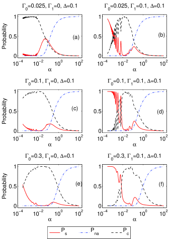
Figure 4: Open-multistate model: Long-time probabilities to occupy the diabats $|0\rangle$ (dashed-dotted) and $|1\rangle$ (full), or the continuum of states (dashed).

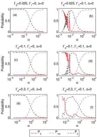
Figure 5: Open-multistate model: Continuum assisted transfer between the diabats with $\Delta=0$.

III.1 Open (multistate) LZ model

We time-evolve the dynamics under the Hamiltonian (4) from the initial state $|0\rangle$ and explore the long-time survival probability in the ground diabatic state, and the probability of nonadiabatic transition, as a function of the sweep rate. Unless otherwise mentioned we use $\Delta=0.1$. The continuum includes $41$ states extending $D=\pm 0.5$ with a constant density of states. In our simulations we set $\Gamma_{n}$ as an energy independent parameter, and from this hybridization energy we resolved the individual coupling strengths using the relation $v_{n,k}=\sqrt{\Gamma_{n}/2\pi\rho}$ from Eq. (5). Similar to the notation typically used in the isolated case, here $P_{s}=P_{0\rightarrow 1}$ stands for the long-time survival probability in the lowest energy diabat and $P_{na}=P_{0\rightarrow 0}$ describes the nonadiabatic transition probability. Furthermore, we define the component residing inside the continuum as $P_{c}=1-P_{s}-P_{na}$.

The behavior of $P_{na}$ is displayed in Fig. 2. It is notable that the value of $\Gamma_{1}$ does not affect this probability. Furthermore, the behavior of $P_{na}$ as a function of sweep rate retains the typical LZ form apart from a shift dependent on $\Gamma_{0}$. In the case of a dense continuum we confirm numerically that this shift corresponds to multiplication by an exponential prefactor function,

$$P_{na}^{shift} = \exp\left(-\frac{4D\Gamma_{0}}{\alpha}\right)P_{na}^{iso}$$ (14)

$$= \exp\left(-\frac{2\pi\Delta^{2}+4D\Gamma_{0}}{\alpha}\right)$$

We can qualitatively justify this form by considering individual-independent pairwise LZ transitions, between the diabat $|0\rangle$ and $|1\rangle$, and between $|0\rangle$ and each continuum state. These transitions happen in succession as the level $|0\rangle$ moves closer in energy to other levels.

More quantitatively, Eq. (14) can be justified using simple semiclassical arguments as follows: Population relaxation into the continuum begins at time $t_{i}$ when the adiabatic states reach the lower threshold of the continuum $-D\sim-\sqrt{\Delta^{2}+[(\alpha t_{i})/2]^{2}}$. This relaxation is completed at $t_{f}$, defined from $D\sim\sqrt{\Delta^{2}+[(\alpha t_{f})/2]^{2}}$. Under the assumption that $\Delta<D$, valid in our simulations, the overall time available for relaxation to the continuum is given by $\tau_{R}\equiv t_{f}-t_{i}\sim 4D/\alpha$. During this time, population relaxation takes place at the rate $\Gamma_{0}$. Hence, taking into account the loss to the continuum alone, the probability to remain in the $|0\rangle$ state is given by the semiclassical expression $\sim e^{-4D\Gamma_{0}/\alpha}$. This probability is further modified by the (independent) LZ pairwise transition when $|0\rangle$ and $|1\rangle$ cross; thus overall, the total nonadiabatic transition probability follows the multiplicative form Eq. (14). While this behavior has been observed before in several multistate models DemOsh ; Brundobler ; Nogo ; Sym ; Sinitsyn ; BT ; NBT ; GBT1 ; GBT2 ; SpinBath , it is interesting to emphasize that it is valid not only for well separated states.

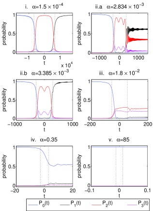
Figure 6: The dynamics of the open-multistate Landau-Zener model in the distinct regimes identified in figure 3(d): (i) adiabatic, (ii) oscillatory, where we follow the dynamics with a velocity corresponding to (ii.a) a minimum in $P_{s}$ or (ii.b) a maximum, (iii) strong depletion, (iv) transitionary, and (v) diabatic regime. Simulations were performed with $\Delta=0$ and $\Gamma_{1}=\Gamma_{0}=0.1$. Plotted are the population of the two diabats, $P_{0}(t)$ and $P_{1}(t)$ and the population of the two lowest-lying continuum levels $P_{2}(t)$ and $P_{3}(t)$. The dotted lines identify the times $t_{i,f}=\mp 2D/\alpha$, when the adiabatic states (approximately) touch the lower and upper continuum threshold.

While nonadiabatic transition probabilities follow the simple shifted LZ form Eq. (14), the ground state survival probability shows a complex behavior due to the influence of the continuum of states as shown in Fig. 3. Our method reproduces the expected Landau-Zener survival probabilities Eq. (3) in the closed case (dashed curve). When $\Gamma_{n}\neq 0$, the numerical solution takes on an entirely different functional form, displaying an oscillatory regime as a function of $\alpha$ with alternating maximum and minimum probabilities.

In the isolated LZ model the solution (3) can be divided into three regimes: the adiabatic regime $\alpha\ll\Delta^{2}$, the counter, diabatic regime $\alpha\gg\Delta^{2}$, and a transitionary regime for $1<\alpha/\Delta^{2}<10^{2}$. The open LZ model shows two additional characteristics at low-intermediate adiabatic rates: an “oscillatory regime” ($\alpha/\Delta^{2}\sim 0.1$), followed by a “strong depletion” phase $\alpha/\Delta^{2}\sim 1$. We assign these five distinct regimes as shown in Fig. 3(d) as (i) adiabatic, (ii) oscillatory, (iii) strong depletion, (iv) transitionary, and (v) diabatic.

A more complete picture of the open model may be reached by simultaneously considering the probabilities of the system being found in $|\,{0}\,\rangle$, $|\,{1}\,\rangle$, or in the continuum states $\left\{|\,{2}\,\rangle,\ldots,|\,{N+1}\,\rangle\right\}$. In Fig. 4 we plot the long-time probabilities $P_{s}=P_{0\rightarrow 1}$, $P_{na}=P_{0\rightarrow 0}$, and $P_{c}=\sum_{j=2}^{N+1}P_{0\rightarrow j}$, for residing in the continuum. We make the following observations: (A) The oscillatory behavior of $P_{s}$ is strong when $\Gamma_{1}\neq 0$; increasing the value of $\Gamma_{0}$ largely affects these features. (B) Both the oscillatory regime and the strong depletion regime result from the system remaining in the continuum rather than making a further nonadiabatic transition to the other diabat for some $\alpha$ values. Furthermore, we show in Fig. 5 that the oscillatory structure is in fact preserved for $\Delta=0$, even maintaining nearly the same values for the transition velocities. (C) When $\Gamma_{1}=0$, the survival probability at low values of $\alpha$ increases with $\Gamma_{0}$, which is an evidence for the presence of cotunelling processes in the system, see panels (a), (c) and (e) in Fig. 4. (D) The shift in the nonadiabatic transition probabilities as described beneath Eq. (14) results from an increased occupation in the continuum, rather than from an increase in probability of finding the system in the other diabatic state.

To understand the complex behavior of the survival probability in the different regimes we choose several specific values of $\alpha$ from Fig. 5 and examine the time evolution across the transition region in detail. This is illustrated in figure 6 using parameter values $\Delta=0$ and $\Gamma_{0}=\Gamma_{1}=0.1$. Recall as discussed above that the oscillatory regime occurs here independently of $\Delta$. Inspecting Fig. 6 we confirm that the continuum begins to participate in the dynamics, in agreement with the semiclassical estimate, when $\epsilon_{0}$ enters the continuum at $t_{i}=-2D/\alpha$. At $t_{f}=2D/\alpha$ the diabats depart from the continuum, and their populations begin to relax to the respective asymptotic values. These times are marked by dotted lines in Fig. 6.

Inspecting the behavior at very low sweep velocities (Region i in Fig. 6) we find that the population is transferred almost entirely from $|\,{0}\,\rangle$ to the lowest-energy continuum state $|\,{2}\,\rangle$ at the beginning of the transition region. Furthermore, the oscillations in the dynamics, after the transition, have sufficient time to damp out. At the last stage, around the time $t_{f}$ the continuum level $|2\rangle$ slowly crosses the diabat $|1\rangle$ and its population is transferred entirely to the state $|\,{1}\,\rangle$. This creates a new, $\Delta$-independent adiabatic regime, governed by a continuum-assisted adiabatic transition, explaining the observation of a finite adiabatic survival probability even with $\Delta=0$.

We now aim to explain the oscillatory Region ii. In Fig. 6(ii.a) and (ii.b) we observe that the time evolution of the continuum states is itself oscillatory, with a specific frequency that is $\alpha$-independent. Maxima in the asymptotic survival probability occur when the continuum-interaction duration $\tau_{R}=4D/\alpha$ is commensurate with the period of this frequency.

Note that the oscillations observed in Fig. 6 are not unique to the continuum states, rather they are a characteristic of the LZ transition, and are seen near the transition region of any pairwise crossing before damping out to the asymptotic limit. In the closed LZ model these oscillations decrease both in period and amplitude as they are damped to a constant value. In addition, their frequency is dependent on the coupling constant $\Delta$. The decrease in period is not observed in the oscillatory regime in the present case as $\tau_{R}$ is sufficiently short, such that the period damping is insignificant. Note that at these low sweep velocities significant population is transferred to the lowest energy states of the continuum, resulting in a very low transfer of population to higher continuum states in subsequent crossings. This explains the similar behavior of the model either with or without $\Delta$, as demonstrated in the comparison between Fig. 4 and Fig. 5.

Next, we explain the depletion region (iii) when $\alpha/\Delta^{2}\sim 1$. For such velocities the continuum levels approach their stationary-asymptotic limit during $\tau_{R}$, as in the usual two-state LZ dynamics. For even higher velocities $\alpha/\Delta^{2}>1$, all continuum states gain population, albeit to a very small extent, thus the survival probability approaches (region iv) and then recovers (region v) the standard LZ curve.

III.2 Stochastic and dissipative LZ models

In this section we explore principal signatures of energy dissipation and thermal excitations in the LZ transition rate and show that these characteristics can be separated from the effect of competing channels as described in Sec. III.1.

We simulate the LZ model with Markovian-Gaussian energy fluctuations, Eq. (9), and display these results in Fig. 7. We use $\Delta=0.1$ and apply the noise only when the diabats satisfy the condition $|\epsilon_{0}(t)-\epsilon_{1}(t)|<\omega_{c}$ with $\omega_{c}=1$. The characteristic transition time is longer than the noise decorrelation time, $\tau_{tr}\sim 2\pi/\Delta\gg\tau_{c}$, $\tau_{c}=\omega_{c}^{-1}\sim 1$. Further, since we only work in the weak coupling limit, $\kappa^{2}\tau_{c}\ll 1$, we can perform our simulations using a Markovian (delta function) correlation function. The behavior observed in Fig. 7 is in agreement with Kayanuma’s results Kayanuma-stoA , displaying a nonmonotonic behavior with an optimal velocity for survival in the low $\kappa$ limit, while reducing to the LZ formula (scaled by a factor of $\frac{1}{2}$) when $\kappa$ is made larger. Note that $P_{na}=1-P_{s}$ for the stochastic model, since population leakage is not allowed.

Fig. 8 shows histograms of $P_{s}$ at different sweep rates, and for small ($\kappa=0.01$) and large ($\kappa=0.2$) noise values, based on 2000 stochastic realizations. As expected, in the diabatic (high velocity) regime weak and strong noise processes lead to similar results for the probability distribution of the survival probability. However, at intermediate-to-small sweep rates ($\alpha/\Delta^{2}<1$) we find marked deviations: For large $\kappa$ the distribution seems uniform in the range $[0,1]$, trivially providing the mean $P_{s}(\alpha=10^{-4})\sim 0.5$. In contrast, at small $\kappa$ the distribution seems to follow an exponential form.

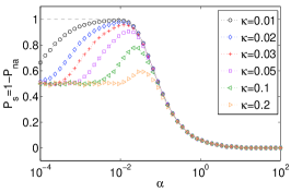
Figure 7: Stochastic LZ model: Probability for survival $P_{s}$, to stay on the ground state at long time, $\kappa=0.01,0.02,0.03,0.05,0.1,0.2$ top to bottom. The dashed line stands for the closed model, $\kappa=0$. In all cases $\Delta=0.1$.

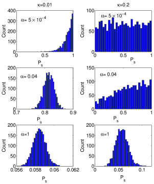
Figure 8: Stochastic LZ model: Histogram of the survival $P_{s}$ probability, to stay on the ground state at long time, $\kappa=0.01$ (left panels) and $\kappa=0.2$ (right panels), with $\alpha=5\times 10^{-4}$, 0.04 and 1, top to bottom. In all cases $\Delta=0.1$.

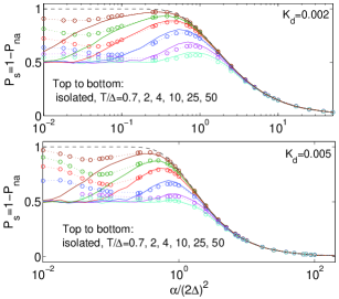
Figure 9: LZ survival probability in the stochastic model (full) and the dissipative case for $T/\Delta=0.7,2,4,10,25,50$ (top-to-bottom, $\circ$). The dashed line stands for the LZ formula (3). (a) Kondo parameter $K_{d}=0.002$, (b) $K_{d}=0.005$. Other QUAPI parameters are $\omega_{c}=20\Delta$ and $\Delta=0.1$. In the stochastic description the variance was prepared from the relation $\kappa=2\sqrt{K_{d}T}$.

The stochastic model emulates the effect of an environment within a fluctuating field, and one should question whether this type of modeling is (at least) qualitatively correct. This issue is addressed in Fig. 9, in which the LZ dynamics of the dissipative model are studied numerically-exactly using the QUAPI technique Makri , as explained in Ref. Thorwart . We used a large cutoff $\omega_{c}=20\Delta$, a small Kondo parameter $K_{d}=0.002-0.005$ and a range of intermediate-high temperatures $T/\Delta=1-50$. QUAPI simulations are aligned with the stochastic model (9) by employing the relation $\kappa=2\sqrt{K_{d}T}$, see Sec. II.3. This translates to noise amplitudes extending the range $\kappa=0.07-1$. We display our results in Fig. 9 in the same format as in Ref. Thorwart , to allow for a quick comparison. We find that the peak in the survival probability with velocity is correctly captured (position, height) within the stochastic model for high-to-intermediate temperatures in the $T/\Delta=1-50$ range. At small sweep velocities $\alpha/\Delta^{2}<0.1$ marked deviations appear: Stochastic simulations approach the probability $P_{s}=1/2$, representing an infinite-temperature bath, while the QUAPI method indicates that the two levels adjust their population to the thermal distribution as dictated by the temperature and the instantaneous energy gap. For higher velocities, $\alpha/\Delta^{2}>0.1$, relaxation with respect to the instantaneous gap is not reached, and the effect of the temperature and the coupling strength can be apparently captured within a single parameter $\kappa$, characterizing energy fluctuations.

It is interesting to note that the two techniques (QUAPI and stochastic simulations) converge in counter manners. QUAPI is easy to converge at high temperatures when the bath decorrelation time is short Makri . In contrast, at high temperatures the noise processes suffers from a high variance, $\kappa^{2}\propto T$, thus stochastic simulations necessitate significant averaging.

III.3 Multistate-stochastic model

We have learned in Sections III.1 and III.2 that population decay from the diabats to other states and energy dissipation processes have distinct effects on the LZ tunneling probabilities. When energy exchange with an environment is permitted, in the form of a stochastic noise, $P_{na}$ acquires a finite value at low sweep rates and a minimum value of $\frac{1}{2}$ in the high $\kappa$ limit, which essentially eliminates the adiabatic limit, see Fig. 7 (with $P_{na}=1-P_{s}$). In contrast, when other channels are included $P_{na}$ simply shows a positive shift in the velocity coordinate (recall Fig. 2). More interesting is the effect of the environment on the survival probability. Allowing energy dissipation in the form of stochastic noise introduces relatively straightforward non-monotonic behavior at low $\kappa$ values, and simply scales the LZ formula at high $\kappa$, Fig. 7. In contrast, the introduction of a resolved continuum displays rich features at low-intermediate sweep velocities, as in Fig. 3. It is essential to probe whether these fine details would survive when interactions with a dissipative environment are in effect.

We address this issue by adjoining to the open-multistate model Eq. (4) a stochastic noise term affecting the energies of the diabats, as in Eq. (9); see the scheme in Fig. 10(a). Results are displayed in Fig. 10(b)-(c) for $\kappa=0.03$. This value could correspond to $K_{d}=0.001$ and $T=0.25$ in the genuine many-body model. For such parameters stochastic simulations are expected to be physically meaningful beyond the strict adiabatic limit, once $\alpha/\Delta^{2}>0.1$, see Fig. 9.

We find that the nonadiabatic transition probability in the open system is entirely shielded from the application of the noise, and it only displays the shift characteristic to the effect of the continuum on the original LZ behavior as in Eq. (14). The survival probability is susceptible to the noise in the adiabatic regime leading to some loss, but the oscillations at low sweep rates and other open-system features are all excellently protected from the noise in comparison to the case without the continuum.

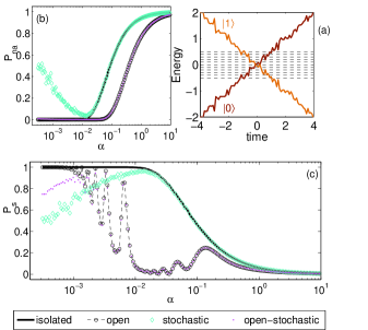
Figure 10: (a) Scheme of the open-stochastic LZ model. (b) Nonadiabatic transition probability $P_{0\rightarrow 0}$ and (c) Survival probability $P_{0\rightarrow 1}$ for the isolated LZ model [Eq. (1), full], open-multistate model [Eq. (4), $\circ$], stochastic LZ model [Eq. (9), $\diamond$], and the open-stochastic case (dotted). Parameters are $\Delta=0.1$, $\Gamma_{0}=\Gamma_{1}=0.1$, $D=\pm 0.5$ and $\kappa=0.03$.

IV Conclusions

Nonadiabatic level crossings are affected by the presence of other channels, discrete or dense, and by energy dissipation and thermal excitation processes induced by the surrounding environment. When inspecting the ground state survival probability and the nonadiabatic transition probability and noting deviations from Eq. (3), can we pinpoint the physical mechanism responsible for these deviations?

To address this problem we have focused in this paper on the open-multistate LZ model of Fig. 1(a) including two diabats and a shared discretized continuum. Using numerical simulations, we have developed a simple analytic expression for the probability of nonadiabatic transition Eq. (14), which is supported by semiclassical considerations of the relaxation time to the continuum. This expression preserves the functional form of the closed LZ formula while simply applying a shift along the sweep velocity coordinate. In contrast, the ground state survival probability at long time manifests an entirely different non-monotonic functional form in the presence of a continuum, with several features that are not present in the original LZ model. The most striking of these features is the presence of an oscillatory regime at low sweep velocities and the onset of a novel continuum-facilitated adiabatic regime. We have explained these features by referring to the dynamics of the original closed LZ problem and by considering the individual transitions between the various states as quasi-independent. Specifically, a continuum-facilitated adiabatic regime replaces the original $\Delta$-dependent regime, and operates through a different mechanism: The probability is transferred from the initial diabatic state to the continuum, and then back to the other diabatic state as illustrated in Fig. 6(i). Meanwhile, the oscillatory regime has been explained with respect to the commensurability of the relaxation time and the period of the oscillations observed in the continuum occupation probabilities near the transition time.

We have complemented the study of the multistate model by considering two other environment-affected LZ models: the stochastic LZ model in which the energy of the diabats fluctuates around the original value, and a more fundamental model in which the diabats couple to a harmonic environment at finite temperature. These models allow for energy exchange processes, reflected by a maxima in the survival probability around $\alpha/\Delta^{2}\sim 1$, and a modification to the deep adiabatic limit, to approach a thermal distribution ratio. Realizations are anticipated in studies of reactions on or close to surfaces Tully1 ; Tully2 , in the field of LZ interferometry, a sensitive tool that can decipher the details of the environment affecting a double-quantum dot system KohlerE , and in other adiabatic devices, where gated quantum dots may indirectly couple CTAP ; Kohler ; Gurvitz , to facilitate population transfer.

In conclusion, in order to identify factors affecting transitions at avoided level crossings one should review both the nonadiabatic transition probability and the survival probability, as they may reveal distinctive features when multichannels are involved. We have also provided numerical evidence that the presence of a continuum may act to shield the nonadiabatic transition probability from the effect of a Gaussian noise, leaving only a definite, predictable shift. This may provide a fertile ground for the development of novel shielding techniques in quantum adiabatic computing QAdi ; AdComp .

- (1) C. Zener, Proc. R. Soc. A. 137, 696 (1932).
- (2) L.D. Landau, Phys. Z. Sowjetunion 2, 46 (1932).
- (3) E.C.G. Stueckelberg, Helv. Phys. Acta 5, 369 (1932).
- (4) E. Majorana, Nuovo Cimento 9, 43 (1932).
- (5) A. Nitzan, Chemical Dynamics in Condensed Phases (Oxford University Press, Oxford 2006).
- (6) T. Köhler, K. Goral, and P, S. Julienne, Rev. Mod. Phys. 78, 1311 (2006).
- (7) I. Chiorescu, P. Bertet, K. Semba, Y. Nakamura, C. J. P. M. Harmans, and J. E. Mooij, Nature 431, 159 (2004).
- (8) A. Wallraff, D. I. Schuster, A. Blais, L. Frunzio, R.- S. Huang, J. Majer, S. Kumar, S. M. Girvin, and R. J. Schoelkopf, Nature 431, 162 (2004).
- (9) W. Wernsdorfer and R. Sessoli, Science 284, 133 (1999).
- (10) A. Zenesini, H. Lignier, G. Tayebirad, J. Radogostowicz, D. Ciampini, R. Mannella, S. Wimberger, O. Morsch, and E. Arimondo, Phys. Rev. Lett. 103, 090403 (2009).
- (11) T. Oka, Phys. Rev. B 86, 075148 (2012).
- (12) S. Longhi and G. Della Valle, Phys. Rev. A 86, 043633 (2012).
- (13) E. Farhi, J. Goldstone, S. Gutmann, and M. Sipser, arXiv:quant ph/0001106
- (14) E. Farhi, J. Goldstone, S. Gutmann, J. Lapan, A. Lundgren, and D. Preda, Science 292, 472 (2001).
- (15) S.N. Shevchenko, S. Ashhab, and F. Nori, Phys. Rep. 492, 1 (2010).
- (16) Y. N. Demkov and V. I. Osherov, Zh. Exsp. Teor. Fiz. 53, 1589 (1967) [Sov. Phys. JETP 26, 916 (1968)].
- (17) S. Brundobler and V. Elser, J. Phys. A Math. Gen. 26, 1211 (1993).
- (18) N. A. Sinitsyn, J. Phys. A Math. Gen. 37, 10691 (2004).
- (19) N. A. Sinitsyn, Phys. Rev. A 87, 032701 (2013).
- (20) N. A. Sinitsyn, Phys. Rev. Lett. 110, 150603 (2013).
- (21) C. Carrol and F. T. Hioe, J. Opt. Soc. Am. B 2, 1355 (1985).
- (22) V. N. Ostrovsky and H. Nakamura, J. Phys. A: Math. Gen. 30, 6939 (1997).
- (23) Yu. N. Demkov and V. N. Ostrovsky, Phys. Rev. A 61, 032705 (2000).
- (24) Yu. N. Demkov and V. N. Ostrovsky, J. Phys. B At. Mol. Opt. 34, 2419 (2001).
- (25) N. A. Sinitsyn and N. Prokof’ev, Phys. Rev. B 67, 134403 (2003).
- (26) V. M. Akulin and W. P. Schleich, Phys. Rev. A 46, 4110 (1992).
- (27) C. A. Moyer, Phys. Rev. A 64, 033406 (2001).
- (28) Y. Avishai and Y. B. Band, arXiv:1311.3919.
- (29) M. Tsukada, J. Phys. Soc. Jpn 51, 2927 (1982).
- (30) Y. Gefen, E. Ben-Jacob, and A. O. Caldeira, Phys. Rev. B 36, 2770 (1987).
- (31) P. Ao and J. Rammer, Phys. Rev. B 43, 5397 (1991)
- (32) E. Shimshoni and A. Stern, Phys. Rev. B 47, 9523 (1993).
- (33) Y. Kayanuma and H. Nakayama, Phys. Rev. B 57 13099 (1998).
- (34) V. L. Pokrovsky and D. Sun, Phys. Rev. B 76, 024310 (2007).
- (35) D. A. Garanin, R. Neb, and R. Schilling, Phys. Rev. B 78, 094405 (2008).
- (36) R. S. Whitney, M. Clusel, and T. Ziman, Phys. Rev. Lett. 107, 210402 (2011).
- (37) M. Wubs, K. Saito, S. Kohler, P. Hänggi, and Y. Kayanuma, Phys. Rev. Lett. 97, 200404 (2006); K. Saito, M. Wubs, S. Kohler, Y. Kayanuma, and P. Hänggi, Phys. Rev. B 75, 214308 (2007).
- (38) P. Nalbach, M. Thorwart, Phys. Rev. Lett. 103, 220401 (2009), Chem. Phys. 375, 234 (2010).
- (39) P. P. Orth, A. Imambekov, and K. Le Hur, Phys. Rev. A 82, 032118 (2010); Phys. Rev. B 87, 014305 (2013).
- (40) A. M. Wodtke, J. C. Tully, and D. J. Auerbach, Int. Reviews in Phys. Chem., 23, 513 (2004).
- (41) N. Shenvi, S. Roy, and J. C. Tully, Science 326, 829 (2009).
- (42) A. D. Greentree, J. H. Cole, A. R. Hamilton, and L. C. L. Hollenberg, Phys. Rev. A 70, 235317 (2004).
- (43) J. Huneke, G. Platero, and S. Köhler, Phys. Rev. Lett. 110, 036802 (2013).
- (44) J. Ping, X.-Q. Li, and S. Gurvitz, Phys. Rev. A 83, 042112 (2011).
- (45) Y. Kayanuma, J. Phys. Soc. Jpn. 53, 108 (1984); 53, 118 (1984); 54, 2037 (1985).
- (46) A. M. Dykhne, J. Exptl. Theoret. Phys. 41, 1324 (1961) [Sov. Phys. JETP 14, 941 (1962)]; L. D. Landau and E. M. Lifshitz, Quantum Mechanics (Non-relativistic Theory), 3rd Ed., Butterworth-Heinemann, Burlington (1977).
- (47) C. Wittig, J. Phys. Chem. B 109, 8428 (2005).
- (48) G. E. Uhlenbeck and L. S. Ornstein, Phys. Rev. 36, 823 (1930).
- (49) N. Makri, J. Math. Phys. 36, 2430 (1995).
- (50) K. Dong and N. Makri, Phys. Rev. A 70, 042101 (2004).
- (51) F. Forster, G. Petersen, S. Manus, P. Hänggi, D. Schuh, W. Wegscheider, S. Kohler, and S. Ludwig, arXiv:1309.5907.