An Information-Spectrum Approach to
Weak Variable-Length Source Coding
with Side-Information

Abstract

This paper studies variable-length (VL) source coding of general sources with side-information. Novel one-shot coding theorems for coding with common side-information available at the encoder and the decoder and Slepian-Wolf (SW) coding (i.e., with side-information only at the decoder) are given, and then, are applied to asymptotic analyses of these coding problems. Especially, a general formula for the infimum of the coding rate asymptotically achievable by weak VL-SW coding (i.e., VL-SW coding with vanishing error probability) is derived. Further, the general formula is applied to investigating weak VL-SW coding of mixed sources. Our results derive and extend several known results on SW coding and weak VL coding, e.g., the optimal achievable rate of VL-SW coding for mixture of i.i.d. sources is given for countably infinite alphabet case with mild condition. In addition, the usefulness of the encoder side-information is investigated. Our result shows that if the encoder side-information is useless in weak VL coding then it is also useless even in the case where the error probability may be positive asymptotically.

I Introduction

In their landmark paper [1], Slepian and Wolf studied the so-called Slepian-Wolf (SW) coding problem, that is, the problem of lossless source compression with side information available only at the decoder. They showed a surprising result that the infimum of achievable coding rate is the same as the case where the side information is also available at the encoder. While Slepian and Wolf considered i.i.d. correlated sources, Cover [2] generalized their result and showed that the encoder side-information does not improve the coding rate even for stationary and ergodic sources.

On the other hand, when we consider general stationary sources (i.e., stationary but not ergodic sources), we can improve the coding rate if side-information is available not only at the decoder but also at the encoder. Further, the result of Yang and He [3, Theorem 2] implies that, even if side-information is not available at the encoder, we can also improve the coding rate by adopting variable-length (VL) coding, i.e., VL-SW coding outperforms fixed-length (FL) SW coding in general. It should be also pointed out that, even for i.i.d. sources, VL coding improves the error exponent and the redundancy of SW coding [4, 5].

These results raise a question: How does the encoder side-information and/or variable-length coding improve the coding rate in more general setting, where not only the ergodicity but also stationarity does not holds? This question gives us the motivation to investigate VL source coding of general, i.e., non-stationary and non-ergodic, sources with side-information only at the decoder and at both of the encoder and the decoder. Further, we focus on the following fact: in the analysis on stationary sources by Yang and He [3, Theorem 2], the ergodic-decomposition theorem, which implies that a general stationary source can be considered as a mixture of stationary and ergodic sources, plays an important role. Since the information spectrum method developed by Han and Verdú [6, 7] provides a powerful tool to investigating coding problems for mixed sources (see, e.g., [6, Sec. 7.3] and [8]), we adopt an information-spectrum approach in our analysis. Another virtue of an information-spectrum approach is that it allows us to consider coding problem without regard to the blocklength of the code. Hence, we can clearly separate one-shot (non-asymptotic) analysis and asymptotic analysis. It brings clarity to the discussion.

I-A Contributions

Our first main contribution is to prove one-shot coding theorems for source coding with common side-information and VL-SW coding. For source coding with common side-information, our coding theorem gives upper and lower bounds on the minimum average codeword length attainable by codes with the error probability less than or equal to $\varepsilon$. Since the difference between the upper and lower bounds is just a constant value, our one-shot coding theorem leads to the optimal coding rate asymptotically achievable by $\varepsilon$-source coding (i.e., coding with the probability of error $\varepsilon_{n}$ satisfying $\limsup_{n\to\infty}\varepsilon_{n}\leq\varepsilon$) with common side-information. For VL-SW coding, we prove direct and converse coding theorems, which show non-asymptotic trade-off between the error probability and the codeword length of VL-SW coding.

Our second main contribution is to derive a general formula for the optimal coding rate asymptotically attainable by weak VL-SW coding, i.e., VL-SW coding with vanishing probability of error $\varepsilon_{n}\to 0$ as the blocklength $n\to\infty$. To characterize the infimum of achievable coding rate, we introduce a novel quantity $H_{\mathrm{s}}(\bm{X}|\bm{Y})$, which is defined by the asymptotic behavior of the conditional entropy-spectrum $(1/n)\log(1/P_{X^{n}|Y^{n}}(X^{n}|Y^{n}))$ of the source $(\bm{X},\bm{Y})=\{(X^{n},Y^{n})\}_{n=1}^{\infty}$. Further, we show relations between $H_{\mathrm{s}}(\bm{X}|\bm{Y})$ and other well known two quantities: our result guarantees that $H_{\mathrm{s}}(\bm{X}|\bm{Y})$ is (i) lower bounded by the conditional sup-entropy rate $\limsup_{n\to\infty}(1/n)H(X^{n}|Y^{n})$ and (ii) upper bounded by the spectral conditional sup-entropy rate $\overline{H}(\bm{X}|\bm{Y})$ [6]. An operational interpretation of this result demonstrates relations among optimal coding rates of three kinds of source coding problems, VL coding with common side-information, weak VL-SW coding, and fixed-length SW coding, of general sources. Moreover, we show that if the source satisfies the conditional strong converse property then those three values are equal.

Further, we consider weak VL-SW coding for mixed sources. We intensively investigate a case where $(\bm{X},\bm{Y})$ is a mixture of two general sources $(\bm{X}_{i},\bm{Y}_{i})$ ($i=1,2$). Although it is not easy to characterize $H_{\mathrm{s}}(\bm{X}|\bm{Y})$ of the mixed source by $H_{\mathrm{s}}(\bm{X}_{i}|\bm{Y}_{i})$ of component sources, we show several properties of $H_{\mathrm{s}}(\bm{X}|\bm{Y})$. Our results spotlights the fundamental importance of distinguishability between two component sources in adjusting the coding rate at the encoder. Roughly speaking, if the encoder, which observes a sequence $x^{n}$, can distinguish between two components, then it can adjust the codeword length assigned to $x^{n}$. Thus, in this case, the optimal rate $H_{\mathrm{s}}(\bm{X}|\bm{Y})$ equals to the average of $H_{\mathrm{s}}(\bm{X}_{i}|\bm{Y}_{i})$ of components. On the other hand, if two marginals $\bm{X}_{1}$ and $\bm{X}_{2}$ are identical, then the encoder cannot distinguish between two components. Hence, the encoder has to set the coding rate sufficiently large so that the decoder can reproduce $x^{n}$ even in the “worst case”. Therefore, in this case, $H_{\mathrm{s}}(\bm{X}|\bm{Y})=\max_{i}H_{\mathrm{s}}(\bm{X}_{i}|\bm{Y}_{i})$ holds. It is not hard to generalize the two components case to the case where the source is a mixture of finite general sources. Our general result derives, as a special case, a formula for the optimal achievable rate of VL-SW coding for mixture of i.i.d. sources with countably infinite alphabets satisfying the uniform integrability.

Our last contribution is to investigate how the encoder side-information helps the coding process. We give a sufficient condition that the encoder side-information does not help $\varepsilon$-coding. Roughly speaking, our result shows that if the encoder side-information is useless in weak VL coding then it is also useless even in $\varepsilon$-VL coding for any $\varepsilon\in(0,1)$.

I-B Related Works

An information-spectrum approach to weak VL coding (without side-information) is initiated by Han [9] (see also [6, Section 1.8]). Subsequently, Koga and Yamamoto [10] investigated $\varepsilon$-VL source coding based on the information-spectrum method. By considering the special case where side-information is constant, we can derive results on weak and $\varepsilon$-VL coding without side-information [9, 10] as a special case of our results in this paper.

Slepian-Wolf coding of general sources was first investigated by Miyake and Kanaya [11] (see also [6, Chapter 7]), where fixed-length SW coding is considered. It can be shown that, in contrast to stationary and ergodic case, VL coding with common side-information outperforms fixed-rate SW coding in general [12]. Our result guarantees that VL-SW coding can attain better performance than fixed-length SW coding but its performance is worse than VL coding with the common side-information.

Variable-length coding for multiterminal sources has been studied well in the context of universal coding, i.e., the encoder and the decoder does not need to know the joint distribution of $(X,Y)$ (e.g., [13, 14]). In the problems of universal variable-length coding for multiterminal sources, it is often assumed that there are links between encoders [15, 16] or the feedback from the decoder to the encoder [17, 3]. In our analysis, we do not assume such a link or feedback.

Variable-length SW coding has been also studied in the context of zero-error source coding, where the probability of error is required to be exactly zero (e.g., [18, 19]). Recall that, for source coding without side-information, the infimum rate achievable by zero-error VL coding is the same as that achievable by weak VL coding, provided that the source satisfies the uniform integrability [6, Theorem 1.8.1]. On the other hand, when side-information is available at the decoder, the requirement of zero-error drastically changes the problem. In this paper, as in [4, 5], we consider only weak VL-SW coding and do not deal with zero-error SW coding.

Recently, analysis of one-shot coding by the information spectrum method attracts a lot of attention as a first step to derive the second order coding rate and/or to investigate the performance in finite blocklength regime (see, e.g., [20, 21, 22, 8, 23]). Our new one-shot coding theorem for VL-SW coding can also be applied to analysis of redundancy of VL-SW coding [5] in a similar manner as [23, 24].

More recently, a large deviations analysis of VL-SW coding problem was given by Weinberger and Merhav [25], where the trade-off between the overflow probability of the coding rate and the error probability at the decode was investigated. Further, Kostina et al. [26] gave non-asymptotic bounds on the minimum average codeword length and the second-order analysis of $\varepsilon$-coding without side-information.

I-C Organization of Paper

In Section II, we introduce our notation and the coding problem investigated in this paper. In Sections III and IV, non-asymptotic coding theorems for coding with common side-information and SW coding are given respectively. Then, we state our general formula for $\varepsilon$-variable length coding with common side-information in Section V. In Section VI, we investigate weakly lossless VL-SW coding and give our general formula. Especially, we give deep investigation on VL-SW coding of mixed-sources. Further, we consider a special case of $\varepsilon$-VL-SW coding in Section VII, where we give a sufficient condition that the encoder side-information is useless. Concluding remarks and directions for future work are provided in Section VIII. To ensure that the main ideas are seamlessly communicated in the main text, we relegate all proofs to the appendices.

II Preliminary

In this section, we introduce our notation and coding systems investigated in this paper.

II-A Notation

Throughout this paper, random variables (e.g., $X$) and their realizations (e.g., $x$) are denoted by capital and lower case letters respectively. All random variables take values in some discrete (finite or countably infinite) alphabets which are denoted by the respective calligraphic letters (e.g., $\mathcal{X}$). Similarly, $X^{n}\triangleq(X_{1},X_{2},\dots,X_{n})$ and $x^{n}\triangleq(x_{1},x_{2},\dots,x_{n})$ denote, respectively, a random vector and its realization in the $n$th Cartesian product $\mathcal{X}^{n}$ of $\mathcal{X}$. For a finite set $\mathcal{S}$, $\left\lvert\mathcal{S}\right\rvert$ denotes the cardinality of $\mathcal{S}$ and $\mathcal{S}^{*}$ denotes the set of all finite strings drawn from $\mathcal{S}$. $\bm{1}$ denotes the indicator function, e.g. $\bm{1}[s\in\mathcal{S}]=1$ if $s\in\mathcal{S}$ and $0$ otherwise. All logarithms are with respect to base 2.

Information-theoretic quantities are denoted in the usual manner [27, 28]. For example, $H(X|Y)$ denotes the conditional entropy of $X$ given $Y$. Moreover, to state our results, we will use quantities defined by using the information-spectrum method [6]. Here, we recall the following probabilistic limit operations. For a sequence $\bm{Z}\triangleq\{Z_{n}\}_{n=1}^{\infty}$ of real-valued random variables, the limit superior in probability of $\bm{Z}$ is defined as

$$\text{p-}\limsup_{n\to\infty}Z_{n} \triangleq\inf\left\{\alpha:\lim_{n\to\infty}\Pr\{Z_{n}>\alpha\}=0\right\}.$$ (1)

Similarly, the limit inferior in probability of $\bm{Z}$ is defined as

$$\text{p-}\liminf_{n\to\infty}Z_{n} \triangleq\sup\left\{\beta:\lim_{n\to\infty}\Pr\{Z_{n}<\beta\}=0\right\}.$$ (2)

In our analyses, the uniform integrability plays a crucial role; See Appendix A for the definition and properties of the uniform integrability. To simplify the statement of results, we abuse the terminology: for a correlated source, i.e., a pair of sequence of random variables $(\bm{X},\bm{Y})\triangleq\{(X^{n},Y^{n})\}_{n=1}^{\infty}$, we say “$(\bm{X},\bm{Y})$ is uniformly integrable” if $\{(1/n)\log(1/P_{X^{n}|Y^{n}}(X^{n}|Y^{n}))\}_{n=1}^{\infty}$ is uniformly integrable.

II-B Coding problems

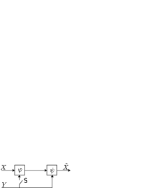
Figure 1: Source coding with common side-information (when the switch $\mathsf{S}$ is closed) and Slepian-Wolf coding (when the switch $\mathsf{S}$ is open)

In this paper, we investigate the source coding system with side-information depicted in Fig. 1. Let $(X,Y)$ be a pair of random variables taking values in $\mathcal{X}\times\mathcal{Y}$ and having joint distribution $P_{XY}$. The sender wishes to communicate the source $X$ via a noiseless link to the receiver with side-information $Y$. We consider two scenarios. In the first scenario, the switch $\mathsf{S}$ in the system Fig. 1 is closed, i.e., the side-information $Y$ is available at both of the sender and receiver as the common side-information. In the other scenario, the switch $\mathsf{S}$ in the system Fig. 1 is open, i.e., the side-information $Y$ is available only at the receiver. The second case is a special (and the most important) case of the coding problem investigated by Slepian and Wolf [1]. So, in this paper, we will call the second case as Slepian-Wolf coding.

III One-Shot Source Coding with Common Side-Information

A variable-length code with common side-information $\Phi=(\varphi,\psi)$ is a pair of mappings that includes an encoder $\varphi\colon\mathcal{X}\times\mathcal{Y}\to\{0,1\}^{*}$ and a decoder $\psi\colon\{0,1\}^{*}\times\mathcal{Y}\to\mathcal{X}$. The output $x\in\mathcal{X}$ of the source with the side-information $y\in\mathcal{Y}$ is encoded by $\varphi$ into the codeword $\varphi(x|y)$. Hereafter, we only consider the case that, for each $y\in\mathcal{Y}$, the set $\mathcal{C}(y)\triangleq\{\varphi(x|y):x\in\mathcal{X}\}\subseteq\{0,1\}^{*}$ of codewords satisfies the prefix condition, i.e., no codewords is a prefix of any other codeword. The length of the codeword $\varphi(x|y)$ is denote by $\ell_{\varphi}(x|y)$. For simplicity, we omit $\varphi$ and write $\ell(x|y)$ if $\varphi$ is apparent from the context. Then, the average codeword length is given by

$$\mathbb{E}\left[\ell(X|Y)\right] \triangleq\sum_{x,y}P_{XY}(x,y)\ell(x|y).$$ (3)

The error probability of the code $\Phi$ is defined as

$$\mathrm{P}_{\mathrm{e}}(\Phi) \triangleq\Pr\left\{X\neq\psi(\varphi(X|Y),Y)\right\}.$$ (4)

A code $\Phi$ is said to be an $\varepsilon$-variable-length code with common side-information (or simply, $\varepsilon$-code) if $\Phi$ satisfies $\mathrm{P}_{\mathrm{e}}(\Phi)\leq\varepsilon$.

The problem is how can we make the average codeword length $\mathbb{E}\left[\ell(X|Y)\right]$ small subject to the constraint $\mathrm{P}_{\mathrm{e}}(\Phi)\leq\varepsilon$. To answer this problem, we introduce some notations.

Given $\mathcal{A}\subseteq\mathcal{X}\times\mathcal{Y}$, let $Q_{XY}^{\mathcal{A}}$ be the distribution defined as

$$Q_{XY}^{\mathcal{A}}(x,y) =\frac{\bm{1}[(x,y)\in\mathcal{A}]}{P_{XY}(\mathcal{A})}P_{XY}(x,y),\quad(x,y)\in\mathcal{X}\times\mathcal{Y}.$$ (5)

Then, we define $H_{\mathcal{A}}(X|Y)$ as the conditional entropy with respect to $Q_{XY}^{\mathcal{A}}$, that is,

$$H_{\mathcal{A}}(X|Y) \triangleq\sum_{(x,y)\in\mathcal{X}\times\mathcal{Y}}Q_{XY}^{\mathcal{A}}(x,y)\log\frac{Q_{Y}^{\mathcal{A}}(y)}{Q_{XY}^{\mathcal{A}}(x,y)}$$ (6)

where $Q_{Y}^{\mathcal{A}}(y)\triangleq\sum_{x}Q_{XY}^{\mathcal{A}}(x,y)$. By using this notation, we define $\varepsilon$-conditional entropy.

Definition 1.

For $0\leq\varepsilon<1$, the $\varepsilon$-conditional entropy of $X$ given $Y$ is defined as

$$H^{\varepsilon}(X|Y) \triangleq\inf_{\begin{subarray}{c}\mathcal{A}\subseteq\mathcal{X}\times\mathcal{Y}:\\ P_{XY}(\mathcal{A})\geq 1-\varepsilon\end{subarray}}P_{XY}(\mathcal{A})H_{\mathcal{A}}(X|Y).$$ (7)

For $\varepsilon=1$, we define $H^{1}(X|Y)=0$.

Remark 1.

$H^{\varepsilon}$ can be considered as a generalized variation of $G_{[\varepsilon]}$ introduced in [10] to investigate $\varepsilon$-source coding without side-information, which is different from $H_{[\varepsilon]}$ introduced by Han [9] to investigate weak variable-length source coding (see [10], [6, Sec. 1.8]).

Now, we give one-shot coding bounds.

Theorem 1 (Coding theorem for one-shot coding with common side-information).

There exists an $\varepsilon$-code satisfying

$$\mathbb{E}\left[\ell(X|Y)\right] \leq H^{\varepsilon}(X|Y)+2.$$ (8)

On the other hand, for any $\varepsilon$-code, we have

$$\mathbb{E}\left[\ell(X|Y)\right] \geq H^{\varepsilon}(X|Y).$$ (9)

Remark 2.

Instead of $H^{\varepsilon}(X|Y)$, let us consider

$$\tilde{H}^{\varepsilon}(X|Y) \triangleq\inf_{\begin{subarray}{c}\mathcal{A}\subseteq\mathcal{X}\times\mathcal{Y}:\\ P_{XY}(\mathcal{A})\geq 1-\varepsilon\end{subarray}}\sum_{(x,y)\in\mathcal{A}}P_{XY}(x,y)\log\frac{1}{P_{X|Y}(x|y)}.$$ (10)

It is easy to prove that

$$\tilde{H}^{\varepsilon}(X|Y)-1\leq H^{\varepsilon}(X|Y)\leq\tilde{H}^{\varepsilon}(X|Y)$$ (11)

holds (see, Appendix B). So, by using $\tilde{H}^{\varepsilon}(X|Y)$, we can give a bound similar as Theorem 1.

Theorem 1 gives a good bound on the optimal average codeword length attainable by $\varepsilon$-codes. However, to calculate $H^{\varepsilon}(X|Y)$ (and/or $\tilde{H}^{\varepsilon}(X|Y)$), we have to optimize the subset $\mathcal{A}\subseteq\mathcal{X}\times\mathcal{Y}$. So, we introduce the other quantity. Let us sort the pairs in $\mathcal{X}\times\mathcal{Y}$ so that $P_{X|Y}(x_{1}|y_{1})\geq P_{X|Y}(x_{2}|y_{2})\geq P_{X|Y}(x_{3}|y_{3})\geq\cdots$. Then, let $i^{*}$ be the integer such that

$$\sum_{i=1}^{i^{*}}P_{XY}(x_{i},y_{i}) \geq 1-\varepsilon$$ (12)

and

$$\sum_{i=1}^{i^{*}-1}P_{XY}(x_{i},y_{i}) <1-\varepsilon.$$ (13)

By using this notation, we define $\hat{H}^{\varepsilon}(X|Y)$ as

$$\hat{H}^{\varepsilon}(X|Y) \triangleq\sum_{i=1}^{i^{*}}P_{XY}(x_{i},y_{i})\log\frac{1}{P_{X|Y}(x_{i}|y_{i})}$$ (14)

$$=H(X|Y)-\sum_{i=i^{*}+1}^{\infty}P_{XY}(x_{i},y_{i})\log\frac{1}{P_{X|Y}(x_{i}|y_{i})}.$$ (15)

Calculation of $\hat{H}^{\varepsilon}(X|Y)$ is easier than that of $H^{\varepsilon}(X|Y)$. Further, by using $\hat{H}^{\varepsilon}(X|Y)$, we can approximate $H^{\varepsilon}(X|Y)$ as follows:

Theorem 2 (Approximation of $H^{\varepsilon}(X|Y)$).

We have

$$\hat{H}^{\varepsilon}(X|Y)-2\leq H^{\varepsilon}(X|Y)\leq\hat{H}^{\varepsilon}(X|Y).$$ (16)

The proof of Theorems 1 and 2 will be given in Appendix B.

By combining Theorem 1 with Theorem 2, we have the following result.

Corollary 1.

There exists an $\varepsilon$-code satisfying

$$\mathbb{E}\left[\ell(X|Y)\right] \leq\hat{H}^{\varepsilon}(X|Y)+2.$$ (17)

On the other hand, for any $\varepsilon$-code, we have

$$\mathbb{E}\left[\ell(X|Y)\right] \geq\hat{H}^{\varepsilon}(X|Y)-2.$$ (18)

IV One-Shot Variable-Length Slepian-Wolf Coding

A code for one-shot variable-length Slepian-Wolf coding is defined in a similar way as in Section III: A code $\Phi=(\varphi,\psi)$ is a pair of mappings that includes an encoder $\varphi\colon\mathcal{X}\to\{0,1\}^{*}$ and a decoder $\psi\colon\{0,1\}^{*}\times\mathcal{Y}\to\mathcal{X}$. We assume that the set $\mathcal{C}\triangleq\{\varphi(x):x\in\mathcal{X}\}\subseteq\{0,1\}^{*}$ of codewords satisfies the prefix condition. The length of the codeword $\varphi(x)$ is denote by $\ell_{\varphi}(x)$ or simply $\ell(x)$. Then, the average codeword length and the error probability are respectively defined as

$$\mathbb{E}\left[\ell(X)\right] \triangleq\sum_{x}P_{X}(x)\ell(x)$$ (19)

and

$$\mathrm{P}_{\mathrm{e}}(\Phi) \triangleq\Pr\left\{X\neq\psi(\varphi(X),Y)\right\}.$$ (20)

A code $\Phi$ is said to be an $\varepsilon$-variable-length Slepian-Wolf code (or simply, $\varepsilon$-SW code) if $\Phi$ satisfies $\mathrm{P}_{\mathrm{e}}(\Phi)\leq\varepsilon$.

To characterize the trade-off between the codeword length and the error probability, we introduce a novel quantity.

Definition 2.

For each $x\in\mathcal{X}$ and $0\leq\varepsilon<1$, let

$$\bar{\mathsf{h}}^{\varepsilon}(x|P_{XY}) \triangleq\inf\left\{\alpha:\sum_{\begin{subarray}{c}y\in\mathcal{Y}:\\ \log\frac{1}{P_{X|Y}(x|y)}>\alpha\end{subarray}}P_{Y|X}(y|x)\leq\varepsilon\right\}.$$ (21)

We will omit $P_{XY}$ and write $\bar{\mathsf{h}}^{\varepsilon}(x)$ if the joint distribution $P_{XY}$ is apparent from the context. For $\varepsilon=1$, we define $\bar{\mathsf{h}}^{1}(x)=0$ for any $x\in\mathcal{X}$.

Remark 3.

The quantity $\bar{\mathsf{h}}^{\varepsilon}(x)$ can be rephrased as follows. Given $x\in\mathcal{X}$, let us define a function $f_{x}$ on $\mathcal{Y}$ so that $f_{x}(y)\triangleq-\log P_{X|Y}(x|y)$. Note that $f_{x}(y)$ can be regarded as the ideal codeword length of $x$ associated with the optimal lossless variable-length code given the common side-information $y$. Further, let $Y_{x}$ be a random variable on $\mathcal{Y}$ such that $\Pr\{Y_{x}=y\}\triangleq P_{Y|X}(y|x)$, and let us consider the probability distribution of $f_{x}(Y_{x})$. Then $\bar{\mathsf{h}}^{\varepsilon}(x)$ can be written as

$$\bar{\mathsf{h}}^{\varepsilon}(x)=\inf\left\{\alpha:\Pr\{f_{x}(Y_{x})>\alpha\}\leq\varepsilon\right\}.$$ (22)

See Fig. 2 for the conceptual image of (22).

Figure 2: Conceptual image of $\bar{\mathsf{h}}^{\varepsilon}(x)$.

Remark 4.

Note that $\log(1/P_{X|Y}(x|y))\geq 0$ and that

$$\sum_{\begin{subarray}{c}y\in\mathcal{Y}:\\ \log\frac{1}{P_{X|Y}(x|y)}>\log\frac{1}{P_{X}(x)}+\log(1/\varepsilon)\end{subarray}}P_{Y|X}(x|y) =\sum_{\begin{subarray}{c}y\in\mathcal{Y}:\\ P_{Y|X}(y|x)<P_{Y}(y)\varepsilon\end{subarray}}P_{Y|X}(y|x)$$ (23)

$$\leq\sum_{\begin{subarray}{c}y\in\mathcal{Y}:\\ P_{Y|X}(y|x)<P_{Y}(y)\varepsilon\end{subarray}}P_{Y}(y)\varepsilon$$ (24)

$$\leq\varepsilon.$$ (25)

By those facts and the definition of $\bar{\mathsf{h}}^{\varepsilon}(x)$, we have

$$0 \leq\bar{\mathsf{h}}^{\varepsilon}(x)\leq\log\frac{1}{P_{X}(x)}+\log\frac{1}{\varepsilon},\quad x\in\mathcal{X},\varepsilon\in(0,1].$$ (26)

On the other hand, if $\varepsilon=0$, we have

$$\bar{\mathsf{h}}^{0}(x) =\sup\left\{\log\frac{1}{P_{X|Y}(x|y)}:y\in\mathcal{Y},P_{Y|X}(y|x)>0\right\}.$$ (27)

By using this quantity, we state our one-shot bounds for $\varepsilon$-SW coding.

Theorem 3 (Direct coding theorem for one-shot SW coding).

Fix $\delta>0$ and $0\leq\varepsilon_{x}\leq 1$ for each $x\in\mathcal{X}$. There exists a code $\Phi$ such that

$$\mathrm{P}_{\mathrm{e}}(\Phi) \leq\sum_{x\in\mathcal{X}}P_{X}(x)\varepsilon_{x}+2^{-\delta/2}$$ (28)

and

$$\ell(x) \leq\bar{\mathsf{h}}^{\varepsilon_{x}}(x)+\delta+2\log\left(\bar{\mathsf{h}}^{\varepsilon_{x}}(x)+\delta+1\right)+3.$$ (29)

Theorem 4 (Converse coding theorem for one-shot SW coding).

For any $\varepsilon$-SW code $\Phi$ and any $\delta>0$, there exists $\varepsilon_{x}\geq 0$ ($x\in\mathcal{X}$) such that

$$\sum_{x\in\mathcal{X}}P_{X}(x)\varepsilon_{x} \leq\varepsilon+2^{-\delta}$$ (30)

and

$$\ell(x) \geq\bar{\mathsf{h}}^{\varepsilon_{x}}(x)-\delta.$$ (31)

Proofs of Theorems 3 and 4 will be given in Appendix C.

Remark 5 (Special case: source coding without side-information).

Let us consider a special case where $\left\lvert\mathcal{Y}\right\rvert=1$, that is, conventional one-to-one variable-rate source coding. In this case, by the definition, we have

$$\bar{\mathsf{h}}^{\varepsilon}(x) =\begin{cases}\log\frac{1}{P_{X}(x)}&0\leq\varepsilon<1,\\ 0&\varepsilon=1.\end{cases}$$ (32)

This fact implies that it is better to set $\varepsilon_{x}$ appearing Theorem 3 so that $\varepsilon_{x}=0$ if the probability $P_{X}(x)$ of $x$ is large and $\varepsilon_{x}=1$ if $P_{X}(x)$ is small. Based on this idea, we can obtain bounds for one-to-one variable-rate source coding. However, the bounds obtained from Theorems 3 and 4 are looser than the bounds obtained from Theorem 1.

V Asymptotic Analysis of Coding with Common Side-Information

In this section, we consider sequences of the coding problem with common side-information indexed by the blocklength $n$ where the sequence $(\bm{X},\bm{Y})\triangleq\{(X^{n},Y^{n})\}_{n=1}^{\infty}$ is general, i.e., we do not place any assumptions on the structure of the source such as stationarity, memorylessness and ergodicity. A code of blocklength $n$ is denoted by $\Phi_{n}=(\varphi_{n},\psi_{n})$. Let $\ell_{n}(x^{n}|y^{n})\triangleq\ell_{\varphi_{n}}(x^{n}|y^{n})$. Given $\varepsilon\in[0,1)$, the $\varepsilon$-achievability of coding rate is defined as follows.

Definition 3.

A rate $R$ is said to be $\varepsilon$-achievable, if there exists a sequence $\{\Phi_{n}\}_{n=1}^{\infty}$ of codes satisfying

$$\limsup_{n\to\infty}\mathrm{P}_{\mathrm{e}}(\Phi_{n}) \leq\varepsilon$$ (33)

and

$$\limsup_{n\to\infty}\frac{1}{n}\mathbb{E}\left[\ell_{n}(X^{n}|Y^{n})\right] \leq R.$$ (34)

Definition 4 (Optimal coding rate achievable by $\varepsilon$-coding with common side-information).

$$R_{com}^{\varepsilon}(\bm{X}|\bm{Y}) \triangleq\inf\left\{R:R\text{ is $\varepsilon$-achievable}\right\}.$$ (35)

We can derive the following coding theorem.

Theorem 5.

For any $\varepsilon\in[0,1)$,

$$R_{com}^{\varepsilon}(\bm{X}|\bm{Y}) =\lim_{\delta\downarrow 0}\limsup_{n\to\infty}\frac{1}{n}H^{\varepsilon+\delta}(X^{n}|Y^{n})$$ (36)

$$=\lim_{\delta\downarrow 0}\limsup_{n\to\infty}\frac{1}{n}\tilde{H}^{\varepsilon+\delta}(X^{n}|Y^{n})$$ (37)

$$=\lim_{\delta\downarrow 0}\limsup_{n\to\infty}\frac{1}{n}\hat{H}^{\varepsilon+\delta}(X^{n}|Y^{n}).$$ (38)

To see the property of $R_{com}^{\varepsilon}(\bm{X}|\bm{Y})$ for some special cases, we give upper and lower bounds on $R_{com}^{\varepsilon}(\bm{X}|\bm{Y})$. Let

$$\overline{H}(\bm{X}|\bm{Y}) \triangleq\text{p-}\limsup_{n\to\infty}\frac{1}{n}\log\frac{1}{P_{X^{n}|Y^{n}}(X^{n}|Y^{n})}$$ (39)

and

$$\underline{H}(\bm{X}|\bm{Y}) \triangleq\text{p-}\liminf_{n\to\infty}\frac{1}{n}\log\frac{1}{P_{X^{n}|Y^{n}}(X^{n}|Y^{n})}.$$ (40)

$\overline{H}(\bm{X}|\bm{Y})$ (resp. $\underline{H}(\bm{X}|\bm{Y})$) is called as the spectral conditional sup-entropy (resp. inf-entropy) rate [6]. Then, we can derive the following bounds.

Theorem 6.

For any $\varepsilon\in[0,1)$,

$$(1-\varepsilon)\underline{H}(\bm{X}|\bm{Y})\leq R_{com}^{\varepsilon}(\bm{X}|\bm{Y})\leq(1-\varepsilon)\overline{H}(\bm{X}|\bm{Y}).$$ (41)

Remark 6.

Let us consider a special case where $\left\lvert\mathcal{Y}\right\rvert=1$. Then, the first inequality of (41) gives the lower bound given in Theorem 4 of [10]. On the other hand, the second inequality of (41) does not give the upper bound given in Theorem 4 of [10]. Further, it is not clear whether our bound is tighter or looser than that of [10] in general. However, by modifying the proof of (41), we can also shows that

$$R_{com}^{\varepsilon}(\bm{X}|\bm{Y}) \leq\inf\{R:F(R|\bm{X},\bm{Y})\leq\varepsilon\}$$ (42)

where

$$F(R|\bm{X},\bm{Y}) \triangleq\limsup_{n\to\infty}\Pr\left\{\frac{1}{n}\log\frac{1}{P_{X^{n}|Y^{n}}(X^{n}|Y^{n})}\geq R\right\}.$$ (43)

See Appendix D. The upper bound (42) can be considered as a special case of the upper bound given in [10].

Now, as a special case, we consider sources for which $(1/n)\log(1/P_{X^{n}|Y^{n}}(X^{n}|Y^{n}))$ concentrates on a single point.

Definition 5 (Conditional strong converse property).

A correlated source $(\bm{X},\bm{Y})=\{(X^{n},Y^{n})\}_{n=1}^{\infty}$ is said to satisfy the conditional strong converse property, if

$$\underline{H}(\bm{X}|\bm{Y})=\overline{H}(\bm{X}|\bm{Y})$$ (44)

holds.

For example, a stationary and ergodic source satisfies the conditional strong converse property. As a corollary of Theorem 6, we have the following result.

Corollary 2.

If $(\bm{X},\bm{Y})$ satisfies the conditional strong converse property then, for any $\varepsilon\in[0,1]$,

$$R_{com}^{\varepsilon}(\bm{X}|\bm{Y}) =(1-\varepsilon)\underline{H}(\bm{X}|\bm{Y})=(1-\varepsilon)\overline{H}(\bm{X}|\bm{Y}).$$ (45)

Proofs of Theorems 5 and 6 will be given in Appendix D.

VI General Formula for Weak Variable-Length Slepian-Wolf Coding

In a similar way as the previous section, we consider SW coding problem for general correlated sources $(\bm{X},\bm{Y})$; we study the codeword length $\ell_{n}(x^{n})\triangleq\ell_{\varphi_{n}}(x^{n})$ associated with a SW-code $\Phi_{n}=(\varphi_{n},\psi_{n})$ of blocklength $n$. Especially, we investigate the weakly lossless case so that the obtained results are meaningful and interpretable.

VI-A General formula

Definition 6.

A rate $R$ is said to be weakly lossless achievable, if there exists a sequence $\{(\varphi_{n},\psi_{n})\}_{n=1}^{\infty}$ of SW-codes satisfying

$$\lim_{n\to\infty}\mathrm{P}_{\mathrm{e}}(\Phi_{n}) =0$$ (46)

and

$$\limsup_{n\to\infty}\frac{1}{n}\mathbb{E}\left[\ell_{n}(X^{n})\right] \leq R.$$ (47)

Definition 7 (Optimal coding rate achievable by weakly lossless SW coding).

$$R_{SW}(\bm{X}|\bm{Y}) \triangleq\inf\left\{R:R\text{ is weakly lossless achievable}\right\}.$$ (48)

To characterize $R_{SW}(\bm{X}|\bm{Y})$, we introduce the following quantity.

Definition 8.

$$H_{\mathrm{s}}(\bm{X}|\bm{Y}) \triangleq\lim_{\varepsilon\downarrow 0}\limsup_{n\to\infty}\frac{1}{n}H_{\mathrm{s}}^{\varepsilon}(X^{n}|Y^{n})$$ (49)

where

$$H_{\mathrm{s}}^{\varepsilon}(X^{n}|Y^{n}) \triangleq\sum_{x^{n}\in\mathcal{X}^{n}}P_{X^{n}}(x^{n})\bar{\mathsf{h}}^{\varepsilon}(x^{n})$$ (50)

and $\bar{\mathsf{h}}^{\varepsilon}(x^{n})=\bar{\mathsf{h}}^{\varepsilon}(x^{n}|P_{X^{n}Y^{n}})$.

Remark 7.

We can choose a sequence $\{\varepsilon_{n}\}_{n=1}^{\infty}$ satisfying that

$$H_{\mathrm{s}}(\bm{X}|\bm{Y}) =\limsup_{n\to\infty}\frac{1}{n}H_{\mathrm{s}}^{\varepsilon_{n}}(X^{n}|Y^{n}).$$ (51)

and that $\varepsilon_{n}\to 0$ and $(1/n)\log(1/\varepsilon_{n})\to 0$ as $n\to\infty$. Such a sequence $\{\varepsilon_{n}\}_{n=1}^{\infty}$ plays an important role in our discussion, especially in proofs of results. We will show this fact as Lemma 5 in Appendix E.

Remark 8.

While the definition of $H_{\mathrm{s}}(\bm{X}|\bm{Y})$ is different from that of $H_{S}(\bm{X}|\bm{Y})$ introduced in [3], $H_{\mathrm{s}}(\bm{X}|\bm{Y})$ can be considered as a generalized variation of $H_{S}(\bm{X}|\bm{Y})$ of [3]: compare our coding theorem (Theorem 7 below) for general sources and Theorem 2 of [3] for stationary souces. Moreover, for a mixture of i.i.d. sources with finite alphabets, we can show that $H_{\mathrm{s}}(\bm{X}|\bm{Y})$ is the same as $H_{S}(\bm{X}|\bm{Y})$ of [3]: see Corollary 5.

Now, we state our general formula.

Theorem 7.

If $(\bm{X},\bm{Y})$ is uniformly integrable then

$$R_{SW}(\bm{X}|\bm{Y}) =H_{\mathrm{s}}(\bm{X}|\bm{Y}).$$ (52)

Remark 9.

A close inspection of the proof reveals that (52) holds under weaker condition. That is, if, for any $\varepsilon\in(0,1)$, $\{\bar{\mathsf{h}}^{\varepsilon}(X^{n})/n\}_{n=1}^{\infty}$ satisfies Condition 2 in Appendix A then (52) holds.

We can give upper and lower bounds on $H_{\mathrm{s}}(\bm{X}|\bm{Y})$ by using well known quantities, the conditional entropy $H(X^{n}|Y^{n})$ and the spectral conditional sup-entropy rate $\overline{H}(\bm{X}|\bm{Y})$ defined in (39).

Theorem 8.

If $(\bm{X},\bm{Y})$ is uniformly integrable then

$$\limsup_{n\to\infty}\frac{1}{n}H(X^{n}|Y^{n})\leq H_{\mathrm{s}}(\bm{X}|\bm{Y})\leq\overline{H}(\bm{X}|\bm{Y}).$$ (53)

Remark 10.

The right-hand side of (53) is the optimal coding rate achievable by fixed-length SW coding [11]. So, the second inequality of (53) is operationally reasonable. On the other hand, the left-hand side of (53) is the optimal coding rate achievable by zero-error VL coding with common side-information. Hence, the first inequality of (53) is slightly stronger than the bound $R_{com}^{0}(\bm{X}|\bm{Y})\leq H_{\mathrm{s}}(\bm{X}|\bm{Y})$. Note that we need the assumption of the uniform integrability of $(\bm{X},\bm{Y})$ in the proof of the first inequality of (53), Lemma 7 in Appendix E. On the other hand, by modifying the proof of Lemma 7, we can show that $R_{com}^{0}(\bm{X}|\bm{Y})\leq H_{\mathrm{s}}(\bm{X}|\bm{Y})$ holds without the assumption that $(\bm{X},\bm{Y})$ is uniform integrable.

Now, assume that $(\bm{X},\bm{Y})$ is uniformly integrable and satisfies the conditional strong converse property. Then, there exists a limit

$$H(\bm{X}|\bm{Y}) \triangleq\lim_{n\to\infty}\frac{1}{n}H(X^{n}|Y^{n})$$ (54)

and it satisfies that $H(\bm{X}|\bm{Y})=\underline{H}(\bm{X}|\bm{Y})=\overline{H}(\bm{X}|\bm{Y})$. Hence, under this condition, (53) of Theorem 8 can be written as

$$H_{\mathrm{s}}(\bm{X}|\bm{Y}) =H(\bm{X}|\bm{Y}).$$ (55)

Actually we can show stronger result.

Theorem 9.

Assume that $(\bm{X},\bm{Y})$ is uniformly integrable and satisfies the conditional strong converse property. Then, for any $\varepsilon\in(0,1)$, we have

$$\lim_{n\to\infty}\frac{1}{n}H_{\mathrm{s}}^{\varepsilon}(X^{n}|Y^{n}) =H(\bm{X}|\bm{Y}).$$ (56)

Proofs of theorems in this subsection, Theorems 7, 8, and 9, will be given in Appendix E.

VI-B Mixed sources

Let us consider two general correlated source $(\bm{X}_{1},\bm{Y}_{1})=\{(X_{1}^{n},Y_{1}^{n})\}_{n=1}^{\infty}$ and $(\bm{X}_{2},\bm{Y}_{2})=\{(X_{2}^{n},Y_{2}^{n})\}_{n=1}^{\infty}$, and let $(\bm{X},\bm{Y})$ be their mixture, i.e., the $n$-th distribution $P_{X^{n}Y^{n}}$ ($n=1,2,\dots$) of $(\bm{X},\bm{Y})$ satisfies

$$P_{X^{n}Y^{n}}(x^{n},y^{n}) \triangleq\alpha_{1}P_{X_{1}^{n}Y_{1}^{n}}(x^{n},y^{n})+\alpha_{2}P_{X_{2}^{n}Y_{2}^{n}}(x^{n},y^{n}),\quad x^{n}\in\mathcal{X}^{n},y^{n}\in\mathcal{Y}^{n}$$ (57)

where $\alpha_{1}$ and $\alpha_{2}$ are constants satisfying $\alpha_{i}>0$ ($i=1,2$) and $\alpha_{1}+\alpha_{2}=1$.

It is well known that $\overline{H}(\bm{X}|\bm{Y})=\max_{i}\overline{H}(\bm{X}_{i}|\bm{Y}_{i})$ [6]. So, Theorem 8 gives an upper bound such as

$$H_{\mathrm{s}}(\bm{X}|\bm{Y})\leq\max_{i}\overline{H}(\bm{X}_{i}|\bm{Y}_{i}).$$ (58)

Similarly, by combining the concavity of the entropy $H(X^{n}|Y^{n})\geq\sum_{i}\alpha_{i}H(X_{i}^{n}|Y_{i}^{n})$ [28] with Theorem 8, we have a lower bound such as

$$H_{\mathrm{s}}(\bm{X}|\bm{Y}) \geq\limsup_{n\to\infty}\sum_{i}\frac{\alpha_{i}}{n}H(X_{i}^{n}|Y_{i}^{n}).$$ (59)

The equalities in (58) and (59) do not necessarily hold in general. Hence, it is not easy to characterize $H_{\mathrm{s}}(\bm{X}|\bm{Y})$ of the mixed source by $H_{\mathrm{s}}(\bm{X}_{i}|\bm{Y}_{i})$ of component sources. In this section, we give a sufficient condition for a mixed source to satisfy $H_{\mathrm{s}}(\bm{X}|\bm{Y})=\max_{i}H_{\mathrm{s}}(\bm{X}_{i}|\bm{Y}_{i})$ and a sufficient condition to $H_{\mathrm{s}}(\bm{X}|\bm{Y})=\sum_{i}\alpha_{i}H_{\mathrm{s}}(\bm{X}_{i}|\bm{Y}_{i})$.

Before stating our result, it should be pointed out that $\bar{\mathsf{h}}^{\varepsilon}(x^{n})=\bar{\mathsf{h}}^{\varepsilon}(x^{n}|P_{X^{n}Y^{n}})$ depends not only on $x^{n}$ and $\varepsilon$ but also the distribution $P_{X^{n}Y^{n}}$ of the source. To specify the dependency on the distribution, let $\bar{\mathsf{h}}_{i}^{\varepsilon}(x^{n})\triangleq\bar{\mathsf{h}}^{\varepsilon}(x^{n}|P_{X_{i}^{n}Y_{i}^{n}})$.

At first, we give a lower bound on $H_{\mathrm{s}}(\bm{X}|\bm{Y})$.

Theorem 10 (Lower bound on $H_{\mathrm{s}}(\bm{X}|\bm{Y})$).

Assume that both of $(\bm{X}_{i},\bm{Y}_{i})$ ($i=1,2$) are uniformly integrable. Then,

$$H_{\mathrm{s}}(\bm{X}|\bm{Y}) \geq\lim_{\varepsilon\downarrow 0}\limsup_{n\to\infty}\sum_{i=1,2}\frac{\alpha_{i}}{n}H_{\mathrm{s}}^{\varepsilon}(X_{i}^{n}|Y_{i}^{n}).$$ (60)

We can give a sufficient condition under which the lower bound given in Theorem 10 is tight. To describe the condition, we use the spectral inf-divergence rate [6] between two marginal sources $\bm{X}_{1}$ and $\bm{X}_{2}$, that is,

$$\underline{D}(\bm{X}_{1}\|\bm{X}_{2}) \triangleq\text{p-}\liminf_{n\to\infty}\frac{1}{n}\log\frac{P_{X_{1}^{n}}(X_{1}^{n})}{P_{X_{2}^{n}}(X_{1}^{n})}.$$ (61)

Theorem 11 (A sufficient condition for tightness of the lower bound).

Assume that both of $(\bm{X}_{i},\bm{Y}_{i})$ ($i=1,2$) are uniformly integrable and that

$$\underline{D}(\bm{X}_{1}\|\bm{X}_{2})>0\text{ and }\underline{D}(\bm{X}_{2}\|\bm{X}_{1})>0.$$ (62)

Then,

$$H_{\mathrm{s}}(\bm{X}|\bm{Y}) =\lim_{\varepsilon\downarrow 0}\limsup_{n\to\infty}\sum_{i=1,2}\frac{\alpha_{i}}{n}H_{\mathrm{s}}^{\varepsilon}(X_{i}^{n}|Y_{i}^{n}).$$ (63)

As a corollary, we can give a condition under which $H_{\mathrm{s}}(\bm{X}|\bm{Y})$ of the mixed source is given as the average of $H_{\mathrm{s}}(\bm{X}_{i}|\bm{Y}_{i})$ of components.

Corollary 3.

Under the assumptions of Theorem 11, if the limit

$$\lim_{n\to\infty}\frac{1}{n}H_{\mathrm{s}}^{\varepsilon}(X_{i}^{n}|Y_{i}^{n})$$ (64)

exists for all sufficiently small $\varepsilon>0$ and $i=1$ and/or $i=2$ then

$$H_{\mathrm{s}}(\bm{X}|\bm{Y}) =\sum_{i=1,2}\alpha_{i}H_{\mathrm{s}}(\bm{X}_{i}|\bm{Y}_{i}).$$ (65)

Next, we give an upper bound on $H_{\mathrm{s}}(\bm{X}|\bm{Y})$.

Theorem 12 (Upper bound on $H_{\mathrm{s}}(\bm{X}|\bm{Y})$).

Assume that both of $(\bm{X}_{i},\bm{Y}_{i})$ ($i=1,2$) are uniformly integrable. Then,

$$H_{\mathrm{s}}(\bm{X}|\bm{Y}) \leq\lim_{\varepsilon\downarrow 0}\limsup_{n\to\infty}\frac{1}{n}\sum_{x^{n}\in\mathcal{X}^{n}}P_{X^{n}}(x^{n})\left[\max_{i}\bar{\mathsf{h}}_{i}^{\varepsilon}(x^{n})\right].$$ (66)

We can show that the upper bound given in Theorem 12 is tight if the marginal distributions of components are identical.

Theorem 13 (A sufficient condition for tightness of the upper bound).

Assume that both of $(\bm{X}_{i},\bm{Y}_{i})$ ($i=1,2$) are uniformly integrable and that $\bm{X}_{1}=\bm{X}_{2}$. Then,

$$H_{\mathrm{s}}(\bm{X}|\bm{Y}) =\lim_{\varepsilon\downarrow 0}\limsup_{n\to\infty}\frac{1}{n}\sum_{x^{n}\in\mathcal{X}^{n}}P_{X^{n}}(x^{n})\left[\max_{i}\bar{\mathsf{h}}_{i}^{\varepsilon}(x^{n})\right].$$ (67)

By Theorem 13, it is apparent that, under the assumptions of the theorem,

$$H_{\mathrm{s}}(\bm{X}|\bm{Y}) \geq\max_{i=1,2}H_{\mathrm{s}}(\bm{X}_{i}|\bm{Y}_{i}).$$ (68)

Hence, by combining (58) and (68), we have the following corollary.

Corollary 4.

Under the assumptions of Theorem 13, if

$$H_{\mathrm{s}}(\bm{X}_{i}|\bm{Y}_{i})=\overline{H}(\bm{X}_{i}|\bm{Y}_{i})$$ (69)

holds for all $i=1,2$ then

$$H_{\mathrm{s}}(\bm{X}|\bm{Y}) =\max_{i=1,2}H_{\mathrm{s}}(\bm{X}_{i}|\bm{Y}_{i})=\max_{i=1,2}\overline{H}(\bm{X}_{i}|\bm{Y}_{i}).$$ (70)

Proofs of Theorems 10, 11, 12, and 13 are given in Appendix F-B.

As shown by Theorem 7, $H_{\mathrm{s}}(\bm{X}|\bm{Y})$ characterizes the optimal coding rate $R_{SW}(\bm{X}|\bm{Y})$ achievable by SW coding. With this observation, let us consider the operational meaning of above results. Recall that the spectral inf-divergence $\underline{D}(\bm{X}_{1}\|\bm{X}_{2})$ characterizes the optimal exponent of the error probability of the second kind in hypothesis testing with $\bm{X}_{1}$ against $\bm{X}_{2}$ [6, Chapter 4]. Roughly speaking, the condition (62) of Theorem 11 means that we can distinguish between two marginal sources $\bm{X}_{1}$ and $\bm{X}_{2}$. So, Theorem 11 implies that if the encoder can distinguish $\bm{X}_{1}$ and $\bm{X}_{2}$ then it can adjust the coding rate, and thus, the average of the optimal coding rates of components can be achieved. On the other hand, Theorem 13 implies that the optimal coding rate $H_{\mathrm{s}}(\bm{X}|\bm{Y})$ is determined by the “worst case” $\max_{i}H_{\mathrm{s}}(\bm{X}_{i}|\bm{Y}_{i})$ of components, if the marginals are identical (and thus the encoder cannot distinguish them).

Remark 11.

The conditions of Theorems 11 and 13 do not cover all cases. Indeed, there exists a pair of general sources $\bm{X}_{1}$ and $\bm{X}_{2}$ for which (62) does not hold while $\bm{X}_{1}\neq\bm{X}_{2}$. However, if both of components are i.i.d. sources with finite alphabet then (62) holds if and only if $\bm{X}_{1}\neq\bm{X}_{2}$.

It is not hard to generalize our results to $m$-components case ($m<\infty$). Let us consider $m$ general sources $(\bm{X}_{i},\bm{Y}_{i})$ ($i=1,\dots,m$) and their mixture

$$P_{X^{n}Y^{n}}(x^{n},y^{n}) =\sum_{i=1}^{m}\alpha_{i}P_{X_{i}^{n}Y_{i}^{n}}(x^{n},y^{n})$$ (71)

where $\alpha_{i}>0$ and $\sum_{i}\alpha_{i}=1$. We have a generalization of two-components case as follows.

Theorem 14.

Assume that all of $(\bm{X}_{i},\bm{Y}_{i})$ ($i=1,2,\dots,m$) are uniformly integrable. Then, following (i) and (ii) hold.

1. If $\underline{D}(\bm{X}_{i}\|\bm{X}_{j})>0$ for all $i\neq j$ and the limit (64) exists for all $i$ and sufficiently small $\varepsilon>0$ then

   $$H_{\mathrm{s}}(\bm{X}|\bm{Y}) =\sum_{i=1}^{m}\alpha_{i}H_{\mathrm{s}}(\bm{X}_{i}|\bm{Y}_{i}).$$ (72)

2. If $\bm{X}_{i}=\bm{X}_{j}$ for all $i,j$ and $H_{\mathrm{s}}(\bm{X}_{i}|\bm{Y}_{i})=\overline{H}(\bm{X}_{i}|\bm{Y}_{i})$ for all $i$ then

   $$H_{\mathrm{s}}(\bm{X}|\bm{Y}) =\max_{i=1,\dots,m}H_{\mathrm{s}}(\bm{X}_{i}|\bm{Y}_{i})=\max_{i=1,\dots,m}\overline{H}(\bm{X}_{i}|\bm{Y}_{i}).$$ (73)

We can prove the theorem by applying Corollaries 3 and 4 repeatedly; See Appendix F-C.

Now, let us recall Theorem 9. It guarantees that if $(\bm{X}_{i},\bm{Y}_{i})$ satisfies the conditional strong converse property then (i) the limit (64) exists for all $\varepsilon\in(0,1)$ and (ii) $H_{\mathrm{s}}(\bm{X}_{i}|\bm{Y}_{i})=H(\bm{X}_{i}|\bm{Y}_{i})=\overline{H}(\bm{X}_{i}|\bm{Y}_{i})$. Hence, as a corollary of Theorem 14, we can derive the following result.

Corollary 5.

Let us consider sources $(\bm{X}_{i},\bm{Y}_{j_{i}})$ ($i=1,\dots,m$ and $j_{i}=1,\dots,m_{i}$) and their mixture:

$$P_{X^{n}Y^{n}}(x^{n},y^{n}) \triangleq\sum_{i=1}^{m}\sum_{j_{i}=1}^{m_{i}}\alpha_{ij_{i}}P_{X_{i}^{n}Y_{j_{i}}^{n}}(x^{n},y^{n})=\sum_{i=1}^{m}\alpha_{i}P_{X_{i}^{n}}(x^{n})\left[\sum_{j_{i}=1}^{m_{i}}\alpha_{j_{i}|i}P_{Y_{j_{i}}^{n}|X_{i}^{n}}(y^{n}|x^{n})\right]$$ (74)

where $\alpha_{ij_{i}}>0$ satisfies $\sum_{i,j_{i}}\alpha_{ij_{i}}=1$ and $\alpha_{i}\triangleq\sum_{j_{i}=1}^{m_{i}}\alpha_{ij_{i}}$ and $\alpha_{j_{i}|i}\triangleq\alpha_{ij_{i}}/\alpha_{i}$. In other words, there are $m$ marginal sources $\bm{X}_{i}$ ($i=1,2,\dots,m$) and for each marginal source there are $m_{i}$ side-information sources $\bm{Y}_{j_{i}}$ ($j_{i}=1,\dots,m_{i}$). We assume that all of $(\bm{X}_{i},\bm{Y}_{j_{i}})$ are uniformly integrable. Further, assume that $(\bm{X}_{i},\bm{Y}_{j_{i}})$ satisfies the conditional strong converse property for all $i$ and $j_{i}$ and that $\underline{D}(\bm{X}_{i}\|\bm{X}_{k})>0$ for all $i\neq k$. Then

$$H_{\mathrm{s}}(\bm{X}|\bm{Y}) =\sum_{i=1}^{m}\alpha_{i}\left[\max_{j_{i}=1,\dots,m_{i}}H(\bm{X}_{i}|\bm{Y}_{j_{i}})\right]$$ (75)

where $H(\bm{X}|\bm{Y})$ is defined in (54).

Remark 12.

Note that under assumptions of Corollary 5, we have

$$H(\bm{X}|\bm{Y}) =\sum_{i=1}^{m}\sum_{j_{i}=1}^{m_{i}}\alpha_{ij_{i}}H(\bm{X}_{i}|\bm{Y}_{j_{i}}),$$ (76)

and

$$\overline{H}(\bm{X}|\bm{Y}) \ =\max_{i,j_{i}}H(\bm{X}_{i}|\bm{Y}_{j_{i}}).$$ (77)

For example, the assumptions of Corollary 5 hold if all components $(\bm{X}_{i},\bm{Y}_{j_{i}})$ are i.i.d. sources with finite alphabets. Note that the finiteness of alphabets is not necessary if sources are uniformly integrable.

VII A Case Where Encoder Side-Information Is Useless

In this section, we give a sufficient condition that the encoder side-information does not help $\varepsilon$-coding. $\varepsilon$-achievability for SW coding is defined in a same way as for coding with common side-information.

Definition 9.

A rate $R$ is said to be $\varepsilon$-achievable, if there exists a sequence $\{(\varphi_{n},\psi_{n})\}_{n=1}^{\infty}$ of SW-codes satisfying

$$\limsup_{n\to\infty}\mathrm{P}_{\mathrm{e}}(\Phi_{n}) \leq\varepsilon$$ (78)

and

$$\limsup_{n\to\infty}\frac{1}{n}\mathbb{E}\left[\ell_{n}(X^{n})\right] \leq R.$$ (79)

Definition 10 (Optimal coding rate achievable by $\varepsilon$-SW coding).

$$R_{SW}^{\varepsilon}(\bm{X}|\bm{Y}) \triangleq\inf\left\{R:R\text{ is $\varepsilon$-achievable}\right\}.$$ (80)

Now, we give a condition and state our result.

Condition 1.

$$\liminf_{n\to\infty}\left[\frac{1}{n}H(X^{n}|Y^{n})-\frac{1}{n}H_{\mathrm{s}}^{\varepsilon_{n}}(X^{n}|Y^{n})\right] \geq 0$$ (81)

where $\{\varepsilon_{n}\}_{n=1}^{\infty}$ is a sequence given in Remark 7.

Theorem 15.

Assume that $(\bm{X},\bm{Y})$ is uniformly integrable. If Condition 1 holds then, for any $\varepsilon\in(0,1)$,

$$R_{SW}^{\varepsilon}(\bm{X}|\bm{Y}) =R_{com}^{\varepsilon}(\bm{X}|\bm{Y}).$$ (82)

Remark 13.

Consider a source $(\bm{X},\bm{Y})$ for which $H(\bm{X}|\bm{Y})=\lim_{n\to\infty}(1/n)H(X^{n}|Y^{n})$ exists. Then the condition (81) is equivalent to $H(\bm{X}|\bm{Y})=H_{\mathrm{s}}(\bm{X}|\bm{Y})$ (Recall the first inequality in (53) of Theorem 8). In other words, in this case, Theorem 15 implies that encoder side-information is useless in $\varepsilon$-coding if it is useless in weakly lossless coding. It should be emphasized that Condition 1 holds and $H(\bm{X}|\bm{Y})=\lim_{n\to\infty}(1/n)H(X^{n}|Y^{n})$ exists even when $(\bm{X},\bm{Y})$ does not satisfy the conditional strong converse property. For example, let us consider the mixed-source given in Corollary 5. If $m_{i}=1$ for all $i$ then the mixed-source satisfies the conditions mentioned above.

VIII Conclusion

In this paper, we gave one-shot and asymptotic coding theorems for VL-SW coding. Especially, VL-SW coding of mixed sources was investigated. In addition, to clarify the impact of the encoder side-information, we also considered VL source coding with common side-information. Our results derives several known results on SW coding, weak and $\varepsilon$-VL coding as corollaries. Moreover, we proved that if the encoder side-information is useless in weak VL coding then it is also useless even in $\varepsilon$-VL coding for any $\varepsilon\in(0,1)$.

On the other hand, some important problems remain as future works:

• Although we can apply Theorems 3 and 4 to investigating asymptotic performance of $\varepsilon$-VL-SW coding, a straightforward application of one-shot bounds may not give meaningful result. To give a general formula for $\varepsilon$-VL-SW coding, from which meaningful results can be derived as corollaries, is an important future work.

• It should be also pointed out that $\varepsilon$-SW coding can be considered as a special case of Wyner-Ziv (WZ) coding [30] (with respect to the distortion measure $d$ such as $d(x^{n},\hat{x}^{n})=1$ if $x^{n}\neq\hat{x}^{n}$ and $d(x^{n},\hat{x}^{n})=0$ if $x^{n}=\hat{x}^{n}$). In this sense, VL-WZ coding with average distortion criteria is a general challenge in the future (While information-spectrum approaches to fixed-length WZ coding are given in [31] and [32], VL-WZ coding has not been reported as long as the authors known).

• While Theorem 15 gives a sufficient condition that the encoder side-information is useless, it is not clear whether Condition 1 is necessary or not. To give a necessary and sufficient condition is an important future work.

• Other future work includes to investigate VL-SW coding with two encoders.

Appendix A Definition and Properties of Uniformly Integrability

A sequence $\{Z_{n}\}_{n=1}^{\infty}$ of real-valued random variables is said to be uniformly integrable (or satisfy the uniform integrability), if $\{Z_{n}\}_{n=1}^{\infty}$ satisfies

$$\lim_{u\to\infty}\sup_{n\geq 1}\sum_{z:\left\lvert z\right\rvert\geq u}P_{Z_{n}}(z)\left\lvert z\right\rvert=0.$$ (83)

It is known that if $\{Z_{n}\}_{n=1}^{\infty}$ is uniformly integrable then it satisfies the following condition (see, e.g. [33]).

Condition 2.

1. There exists $M<\infty$ such that $\mathbb{E}[Z_{n}]<M$ for all $n$.

2. If a sequence $\{\mathcal{A}_{n}\}_{n=1}^{\infty}$ of subsets $\mathcal{A}_{n}\subseteq\mathcal{Z}_{n}$ satisfies $P_{Z_{n}}(\mathcal{A}_{n})\to 0$ as $n\to\infty$ then

   $$\lim_{n\to\infty}\sum_{z\in\mathcal{A}_{n}}P_{Z_{n}}(z)\left\lvert z\right\rvert=0.$$ (84)

While some of our results assume uniform integrability of random variables, only two properties given in Condition 2 are needed in our proof. This fact is important in the analysis of mixed-source in Section VI-B. Let us consider two sources $(\bm{X}_{i},\bm{Y}_{i})$ ($i=1,2$) and the mixture $(\bm{X},\bm{Y})$ of them defined as (57). It is not clear whether the following statement is true: If both of $(\bm{X}_{i},\bm{Y}_{i})$ ($i=1,2$) are uniformly integrable then $(\bm{X},\bm{Y})$ is also uniformly integrable. We have, however, the following lemma.

Lemma 1.

Let us consider two sources $(\bm{X}_{i},\bm{Y}_{i})$ ($i=1,2$) and the mixture of them defined as (57). If both of $\{(1/n)\log(1/P_{X_{i}^{n}|Y_{i}^{n}}(X_{i}^{n}|Y_{i}^{n}))\}_{n=1}^{\infty}$ ($i=1,2$) satisfy Condition 2 then $\{(1/n)\log(1/P_{X^{n}|Y^{n}}(X^{n}|Y^{n}))\}_{n=1}^{\infty}$ also satisfies Condition 2.

Proof:

For $i=1,2$, let $\bar{\imath}=2$ if $i=1$ and $\bar{\imath}=1$ if $i=2$. We have, for any $n$ and $\mathcal{A}_{n}\subseteq\mathcal{X}^{n}\times\mathcal{Y}^{n}$,

$$\frac{1}{n}\sum_{(x^{n},y^{n})\in\mathcal{A}_{n}}P_{X^{n}Y^{n}}(x^{n},y^{n})\log\frac{1}{P_{X^{n}|Y^{n}}(x^{n}|y^{n})}$$

$$=\frac{1}{n}\sum_{i}\sum_{(x^{n},y^{n})\in\mathcal{A}_{n}}\alpha_{i}P_{X_{i}^{n}Y_{i}^{n}}(x^{n},y^{n})\log\frac{\sum_{j}\alpha_{j}P_{Y_{j}^{n}}(y^{n})}{\sum_{k}\alpha_{k}P_{X_{k}^{n}Y_{k}^{n}}(x^{n},y^{n})}$$ (85)

$$\leq\frac{1}{n}\sum_{i}\sum_{(x^{n},y^{n})\in\mathcal{A}_{n}}\alpha_{i}P_{X_{i}^{n}Y_{i}^{n}}(x^{n},y^{n})\log\frac{\sum_{j}\alpha_{j}P_{Y_{j}^{n}}(y^{n})}{\alpha_{i}P_{X_{i}^{n}Y_{i}^{n}}(x^{n},y^{n})}$$ (86)

$$\leq\frac{1}{n}\sum_{i}\Biggl{[}\sum_{\begin{subarray}{c}(x^{n},y^{n})\in\mathcal{A}_{n}\\ P_{Y_{i}^{n}}(y^{n})\geq P_{Y_{\bar{\imath}}^{n}}(y^{n})\end{subarray}}\alpha_{i}P_{X_{i}^{n}Y_{i}^{n}}(x^{n},y^{n})\log\frac{P_{Y_{i}^{n}}(y^{n})}{\alpha_{i}P_{X_{i}^{n}Y_{i}^{n}}(x^{n},y^{n})}$$

$$\qquad+\sum_{\begin{subarray}{c}(x^{n},y^{n})\in\mathcal{A}_{n}\\ P_{Y_{i}^{n}}(y^{n})<P_{Y_{\bar{\imath}}^{n}}(y^{n})\end{subarray}}\alpha_{i}P_{X_{i}^{n}Y_{i}^{n}}(x^{n},y^{n})\log\frac{P_{Y_{\bar{\imath}}^{n}}(y^{n})}{\alpha_{i}P_{X_{i}^{n}Y_{i}^{n}}(x^{n},y^{n})}\Biggr{]}$$ (87)

$$\leq\frac{1}{n}\sum_{i}\Biggl{[}\sum_{(x^{n},y^{n})\in\mathcal{A}_{n}}\alpha_{i}P_{X_{i}^{n}Y_{i}^{n}}(x^{n},y^{n})\log\frac{1}{\alpha_{i}P_{X_{i}^{n}|Y_{i}^{n}}(x^{n}|y^{n})}$$

$$\qquad+\sum_{\begin{subarray}{c}(x^{n},y^{n})\in\mathcal{A}_{n}\\ P_{Y_{i}^{n}}(y^{n})<P_{Y_{\bar{\imath}}^{n}}(y^{n})\end{subarray}}\alpha_{i}P_{X_{i}^{n}Y_{i}^{n}}(x^{n},y^{n})\log\frac{P_{Y_{\bar{\imath}}^{n}}(y^{n})}{P_{Y_{i}}^{n}(y^{n})}\Biggr{]}$$ (88)

$$\stackrel{{\scriptstyle\text{(a)}}}{{\leq}}\frac{1}{n}\sum_{i}\sum_{(x^{n},y^{n})\in\mathcal{A}_{n}}\alpha_{i}P_{X_{i}^{n}Y_{i}^{n}}(x^{n},y^{n})\log\frac{1}{\alpha_{i}P_{X_{i}^{n}|Y_{i}^{n}}(x^{n}|y^{n})}$$

$$\qquad+\frac{1}{n}\sum_{i}\sum_{\begin{subarray}{c}(x^{n},y^{n})\in\mathcal{A}_{n}\\ P_{Y_{i}^{n}}(y^{n})<P_{Y_{\bar{\imath}}^{n}}(y^{n})\end{subarray}}\alpha_{i}P_{X_{i}^{n}Y_{i}^{n}}(x^{n},y^{n})\frac{P_{Y_{\bar{\imath}}^{n}}(y^{n})}{P_{Y_{i}^{n}}(y^{n})}\log\mathrm{e}$$ (89)

$$\leq\frac{1}{n}\sum_{i}\sum_{(x^{n},y^{n})\in\mathcal{A}_{n}}\alpha_{i}P_{X_{i}^{n}Y_{i}^{n}}(x^{n},y^{n})\log\frac{1}{\alpha_{i}P_{X_{i}^{n}|Y_{i}^{n}}(x^{n}|y^{n})}+\frac{\log\mathrm{e}}{n}$$ (90)

$$=\sum_{i}\alpha_{i}\sum_{(x^{n},y^{n})\in\mathcal{A}_{n}}P_{X_{i}^{n}Y_{i}^{n}}(x^{n},y^{n})\left[\frac{1}{n}\log\frac{1}{P_{X_{i}^{n}|Y_{i}^{n}}(x^{n}|y^{n})}\right]+\frac{h_{2}(\alpha_{1})+\log\mathrm{e}}{n}$$ (91)

$$\leq\sum_{i}\alpha_{i}\mathbb{E}\left[\frac{1}{n}\log\frac{1}{P_{X_{i}^{n}|Y_{i}^{n}}(X_{i}^{n}|Y_{i}^{n})}\right]+h_{2}(\alpha_{1})+\log\mathrm{e}$$ (92)

where $h_{2}(p)\triangleq-p\log p-(1-p)\log(1-p)$ and (a) follows from $\log x\leq(x-1)\log\mathrm{e}\leq x\log\mathrm{e}$.

The assumption of the lemma and (92) (resp. (91)) guarantee that $\{(1/n)\log(1/P_{X^{n}|Y^{n}}(X^{n}|Y^{n}))\}_{n=1}^{\infty}$ satisfies the property (i) (resp. (ii)) of Condition 2. ∎

Further, we have also the following lemma.

Lemma 2.

If $\left\{\frac{1}{n}\log\frac{1}{P_{X^{n}|Y^{n}}(X^{n}|Y^{n})}\right\}_{n=1}^{\infty}$ satisfies Condition 2 then, for any $0<\varepsilon\leq 1$, $\left\{\frac{\bar{\mathsf{h}}^{\varepsilon}(X^{n})}{n}\right\}_{n=1}^{\infty}$ also satisfies Condition 2.

Proof:

Fix $\gamma>0$. For any $u\geq 0$ and $x^{n}\in\mathcal{X}^{n}$ such that $\bar{\mathsf{h}}^{\varepsilon}(x^{n})\geq un$, we have

$$\sum_{\begin{subarray}{c}y^{n}\in\mathcal{Y}^{n}:\\ \log\frac{1}{P_{X^{n}|Y^{n}}(x^{n}|y^{n})}>un-\gamma\end{subarray}}P_{Y^{n}|X^{n}}(y^{n}|x^{n})\log\frac{1}{P_{X^{n}|Y^{n}}(x^{n}|y^{n})}$$

$$\geq\sum_{\begin{subarray}{c}y^{n}\in\mathcal{Y}^{n}:\\ \log\frac{1}{P_{X^{n}|Y^{n}}(x^{n}|y^{n})}>\bar{\mathsf{h}}^{\varepsilon}(x^{n})-\gamma\end{subarray}}P_{Y^{n}|X^{n}}(y^{n}|x^{n})\log\frac{1}{P_{X^{n}|Y^{n}}(x^{n}|y^{n})}$$ (93)

$$\geq\sum_{\begin{subarray}{c}y^{n}\in\mathcal{Y}^{n}:\\ \log\frac{1}{P_{X^{n}|Y^{n}}(x^{n}|y^{n})}>\bar{\mathsf{h}}^{\varepsilon}(x^{n})-\gamma\end{subarray}}P_{Y^{n}|X^{n}}(y^{n}|x^{n})\left\{\bar{\mathsf{h}}^{\varepsilon}(x^{n})-\gamma\right\}$$ (94)

$$>\varepsilon\left\{\bar{\mathsf{h}}^{\varepsilon}(x^{n})-\gamma\right\}$$ (95)

where the last inequality follows from the definition of $\bar{\mathsf{h}}^{\varepsilon}(x^{n})$. Thus, we have

$$\bar{\mathsf{h}}^{\varepsilon}(x^{n})\leq\frac{1}{\varepsilon}\sum_{\begin{subarray}{c}y^{n}\in\mathcal{Y}^{n}:\\ \log\frac{1}{P_{X^{n}|Y^{n}}(x^{n}|y^{n})}>un-\gamma\end{subarray}}P_{Y^{n}|X^{n}}(y^{n}|x^{n})\log\frac{1}{P_{X^{n}|Y^{n}}(x^{n}|y^{n})}+\gamma.$$ (96)

On the other hand, by the assumption, we can choose $M<\infty$ so that $\mathbb{E}\left[(1/n)\log(1/P_{X^{n}|Y^{n}}(X^{n}|Y^{n}))\right]\leq M$ for all $n$. Hence, we have, for any $n$ and $\mathcal{A}_{n}\subseteq\mathcal{X}^{n}$,

$$\sum_{x^{n}\in\mathcal{A}_{n}}P_{X^{n}}(x^{n})\frac{\bar{\mathsf{h}}^{\varepsilon}(x^{n})}{n}$$

$$\leq uP_{X^{n}}(A_{n})+\sum_{\begin{subarray}{c}x^{n}\in\mathcal{A}_{n}:\\ \bar{\mathsf{h}}^{\varepsilon}(x^{n})\geq un\end{subarray}}P_{X^{n}}(x^{n})\frac{\bar{\mathsf{h}}^{\varepsilon}(x^{n})}{n}$$ (97)

$$\leq uP_{X^{n}}(A_{n})+\sum_{\begin{subarray}{c}x^{n}\in\mathcal{A}_{n}:\\ \bar{\mathsf{h}}^{\varepsilon}(x^{n})\geq un\end{subarray}}P_{X^{n}}(x^{n})\left[\frac{1}{n\varepsilon}\sum_{\begin{subarray}{c}y^{n}\in\mathcal{Y}^{n}:\\ \log\frac{1}{P_{X^{n}|Y^{n}}(x^{n}|y^{n})}>un-\gamma\end{subarray}}P_{Y^{n}|X^{n}}(y^{n}|x^{n})\log\frac{1}{P_{X^{n}|Y^{n}}(x^{n}|y^{n})}+\frac{\gamma}{n}\right]$$ (98)

$$\leq uP_{X^{n}}(A_{n})+\frac{1}{n\varepsilon}\sum_{x^{n}\in\mathcal{A}_{n}}P_{X^{n}}(x^{n})\sum_{\begin{subarray}{c}y^{n}\in\mathcal{Y}^{n}:\\ \log\frac{1}{P_{X^{n}|Y^{n}}(x^{n}|y^{n})}>un-\gamma\end{subarray}}P_{Y^{n}|X^{n}}(y^{n}|x^{n})\log\frac{1}{P_{X^{n}|Y^{n}}(x^{n}|y^{n})}+\frac{\gamma}{n}$$ (99)

$$=uP_{X^{n}}(A_{n})+\frac{1}{n\varepsilon}\sum_{\begin{subarray}{c}(x^{n},y^{n})\in\mathcal{A}_{n}\times\mathcal{Y}^{n}:\\ \log\frac{1}{P_{X^{n}|Y^{n}}(x^{n}|y^{n})}>un-\gamma\end{subarray}}P_{X^{n}Y^{n}}(x^{n},y^{n})\log\frac{1}{P_{X^{n}|Y^{n}}(x^{n}|y^{n})}+\frac{\gamma}{n}$$ (100)

$$\leq uP_{X^{n}}(A_{n})+\frac{1}{\varepsilon}\sum_{(x^{n},y^{n})\in\mathcal{A}_{n}\times\mathcal{Y}^{n}}P_{X^{n}Y^{n}}(x^{n},y^{n})\left[\frac{1}{n}\log\frac{1}{P_{X^{n}|Y^{n}}(x^{n}|y^{n})}\right]+\frac{\gamma}{n}$$ (101)

$$\leq u+\frac{1}{\varepsilon}\mathbb{E}\left[\frac{1}{n}\log\frac{1}{P_{X^{n}|Y^{n}}(X^{n}|Y^{n})}\right]+\gamma.$$ (102)

The assumption of the lemma and (102) (resp. (101)) guarantee that $\{(1/n)\log(1/P_{X^{n}|Y^{n}}(X^{n}|Y^{n}))\}_{n=1}^{\infty}$ satisfies the property (i) (resp. (ii)) of Condition 2. ∎

Appendix B Proofs of results in Section III

In this appendix, we prove Theorem 1, inequality (11), and Theorem 2.

Proof:

Direct part

Fix $\gamma>0$ arbitrarily and fix $\mathcal{A}\subseteq\mathcal{X}\times\mathcal{Y}$ such that $P_{XY}(\mathcal{A})\geq 1-\varepsilon$ and $P_{XY}(\mathcal{A})H_{\mathcal{A}}(X|Y)\leq H^{\varepsilon}(X|Y)+\gamma$. Let us consider the following coding scheme

• if $(x,y)\in\mathcal{A}$ then the encoder sends one bit flag “0” followed by $x$ encoded by using the Shannon code designed for the conditional probability $Q_{X|Y}^{\mathcal{A}}(x|y)\triangleq Q_{XY}^{\mathcal{A}}(x,y)/Q_{Y}^{\mathcal{A}}(y)$.

• if $(x,y)\notin\mathcal{A}$ then encoder sends only one bit flag “1”.

It is not hard to see that

• $x$ is decoded successfully if $(x,y)\in\mathcal{A}$ and thus the error probability of this scheme is less than or equal to $\varepsilon$.

• the average codeword length is upper bounded by

  $$1+P_{XY}(\mathcal{A})\left[H_{\mathcal{A}}(X|Y)+1\right]\leq P_{XY}(\mathcal{A})H_{\mathcal{A}}(X|Y)+2\leq H^{\varepsilon}(X|Y)+2+\gamma.$$ (103)

Since $\gamma>0$ is arbitrarily, we have (8).

Converse part

Fix $\varepsilon$-code $\Phi=(\varphi,\psi)$ and let $\mathcal{A}\triangleq\{(x,y):x=\psi(\varphi(x|y),y)\}$. It is apparent that, for all $(x,y)\not\in\mathcal{A}$, we can lower bound the codeword length as $\ell(x|y)\geq 0$. On the other hand, for each $y\in\mathcal{Y}$, $\varphi(\cdot|y)$ gives a lossless prefix code on $\mathcal{A}(y)\triangleq\{x:(x,y)\in\mathcal{A}\}$. Hence, by using a standard technique which proves the converse part of the coding theorem for lossless variable-length coding (e.g. [27]), we can show that

$$\sum_{(x,y)\in\mathcal{A}}Q_{XY}^{\mathcal{A}}(x,y)\ell(x|y) \geq H_{\mathcal{A}}(X|Y).$$ (104)

It is not hard to see that (9) follows from (104). ∎

Proof:

Given $\mathcal{A}\subseteq\mathcal{X}\times\mathcal{Y}$, let

$$\mu_{\mathcal{A}}(y) \triangleq\frac{1}{P_{Y}(y)}\left[\sum_{x\in\mathcal{X}}\bm{1}[(x,y)\in\mathcal{A}]P_{XY}(x,y)\right].$$ (105)

Then, we can write

$$Q_{Y}^{\mathcal{A}}(y) =\sum_{x\in\mathcal{X}}Q_{XY}^{\mathcal{A}}(x,y)=\frac{P_{Y}(y)\mu_{\mathcal{A}}(y)}{P_{XY}(\mathcal{A})}$$ (106)

and thus

$$P_{XY}(\mathcal{A})H_{\mathcal{A}}(X|Y) =P_{XY}(\mathcal{A})\sum_{(x,y)\in\mathcal{X}\times\mathcal{Y}}Q_{XY}^{\mathcal{A}}(x,y)\log\frac{Q_{Y}^{\mathcal{A}}(y)}{Q_{XY}^{\mathcal{A}}(x,y)}$$ (107)

$$=\sum_{(x,y)\in\mathcal{A}}P_{XY}(x,y)\log\frac{P_{Y}(y)\mu_{\mathcal{A}}(y)}{P_{XY}(x,y)}$$ (108)

$$=\sum_{(x,y)\in\mathcal{A}}P_{XY}(x,y)\log\frac{\mu_{\mathcal{A}}(y)}{P_{X|Y}(x|y)}.$$ (109)

Since $0\leq\mu_{\mathcal{A}}(y)\leq 1$, we have

$$\sum_{(x,y)\in\mathcal{A}}P_{XY}(x,y)\log\frac{\mu_{\mathcal{A}}(y)}{P_{X|Y}(x|y)} \leq\sum_{(x,y)\in\mathcal{A}}\frac{P_{XY}(x,y)}{P_{XY}(\mathcal{A})}\log\frac{1}{P_{X|Y}(x|y)}.$$ (110)

On the other hand,

$$\sum_{(x,y)\in\mathcal{A}}P_{XY}(x,y)\log\frac{\mu_{\mathcal{A}}(y)}{P_{X|Y}(x|y)} =\sum_{(x,y)\in\mathcal{A}}P_{XY}(x,y)\log\frac{1}{P_{X|Y}(x|y)}+\sum_{(x,y)\in\mathcal{A}}P_{XY}(x,y)\log\mu_{\mathcal{A}}(y)$$ (111)

$$=\sum_{(x,y)\in\mathcal{A}}P_{XY}(x,y)\log\frac{1}{P_{X|Y}(x|y)}+\sum_{y\in\mathcal{Y}}P_{Y}(y)\mu_{\mathcal{A}}(y)\log\mu_{\mathcal{A}}(y)$$ (112)

$$\geq\sum_{(x,y)\in\mathcal{A}}P_{XY}(x,y)\log\frac{1}{P_{X|Y}(x|y)}-\sum_{y\in\mathcal{Y}}P_{Y}(y)$$ (113)

$$=\sum_{(x,y)\in\mathcal{A}}P_{XY}(x,y)\log\frac{1}{P_{X|Y}(x|y)}-1$$ (114)

where the inequality follows from the fact that $p\log p\geq-1$ for $p\in[0,1]$. The inequality (11) follows from (109), (110), (114), and the definitions of quantities. ∎

Proof:

Since (11) holds, it is sufficient to show that

$$\tilde{H}^{\varepsilon}(X|Y)\leq\hat{H}^{\varepsilon}(X|Y)$$ (115)

and

$$\tilde{H}^{\varepsilon}(X|Y)\geq\hat{H}^{\varepsilon}(X|Y)-1.$$ (116)

The first inequality (115) is apparent, since $\mathcal{A}\triangleq\{(x_{i},y_{i}):1\leq i\leq i^{*}\}$ satisfies $P_{XY}(\mathcal{A})\geq 1-\varepsilon$.

On the other hand, by the definition of $\tilde{H}^{\varepsilon}(X|Y)$, we have

$$\tilde{H}^{\varepsilon}(X|Y)\geq\inf_{f}\sum_{(x,y)\in\mathcal{X}\times\mathcal{Y}}P_{XY}(x,y)f(x,y)\log\frac{1}{P_{X|Y}(x|y)}$$ (117)

where $\inf_{f}$ is taken over all functions on $\mathcal{X}\times\mathcal{Y}$ such that

$$0\leq f(x,y)\leq 1$$ (118)

and

$$\sum_{(x,y)\in\mathcal{X}\times\mathcal{Y}}P_{XY}(x,y)f(x,y)\geq 1-\varepsilon.$$ (119)

Note that the right hand side of (117) can be written as a linear programming such as

$$\text{mimimize}\quad\sum_{(x,y)\in\mathcal{X}\times\mathcal{Y}}g(x,y)\log\frac{1}{P_{X|Y}(x|y)}$$ (120)

subject to

$$0\leq g(x,y)\leq P_{XY}(x,y)$$ (121)

and

$$\sum_{(x,y)\in\mathcal{X}\times\mathcal{Y}}g(x,y)\geq 1-\varepsilon.$$ (122)

The solution of this problem is given by $g$ such as

$$g(x_{i},y_{i}) =\begin{cases}P_{XY}(x_{i},y_{i})&i<i^{*},\\ \sum_{i=i^{*}}^{\infty}P_{XY}(x_{i},y_{i})-\varepsilon&i=i^{*},\\ 0&i>i^{*}.\end{cases}$$ (123)

By this fact and the definition of $\hat{H}^{\varepsilon}(X|Y)$, we have

$$\tilde{H}^{\varepsilon}(X|Y) \geq\hat{H}^{\varepsilon}(X|Y)-\left[\varepsilon-\sum_{i=i^{*}+1}^{\infty}P_{XY}(x_{i},y_{i})\right]\log\frac{1}{P_{X|Y}(x_{i^{*}}|y_{i^{*}})}$$ (124)

$$\geq\hat{H}^{\varepsilon}(X|Y)-P_{XY}(x_{i^{*}},y_{i^{*}})\log\frac{1}{P_{X|Y}(x_{i^{*}}|y_{i^{*}})}$$ (125)

$$\geq\hat{H}^{\varepsilon}(X|Y)-P_{XY}(x_{i^{*}},y_{i^{*}})\log\frac{1}{P_{XY}(x_{i^{*}},y_{i^{*}})}$$ (126)

$$\geq\hat{H}^{\varepsilon}(X|Y)-1$$ (127)

and thus, (116) holds. ∎

Appendix C Proofs of Results in Section IV

In this appendix, we prove coding theorems for one-shot SW coding, i.e. Theorems 3 and 4.

Proof:

For each $x\in\mathcal{X}$, let

$$\tilde{\ell}(x) \triangleq\left\lceil\bar{\mathsf{h}}^{\varepsilon_{x}}(x)+\delta\right\rceil.$$ (128)

Further, for each integer $l\in\{\tilde{\ell}(x):x\in\mathcal{X}\}$, prepare a random bin code with $l$-bits bin-index and let

$$\mathcal{T}(l) \triangleq\left\{(x,y):\log\frac{1}{P_{X|Y}(x|y)}\leq l-\frac{\delta}{2}\right\}.$$ (129)

Note that, for all $y\in\mathcal{Y}$,

$$\left\lvert\{x:(x,y)\in\mathcal{T}(l)\}\right\rvert\leq 2^{l-\delta/2}.$$ (130)

Now, we construct the encoder and the decoder as follows:

• Given $x\in\mathcal{X}$, the encoder

  1. sends $\tilde{\ell}(x)$ by using at most $2(\lfloor\log\tilde{\ell}(x)\rfloor+1)$ bits [29], and then

  2. sends the bin-index $m=\mathrm{bin}(x)$ of $x$ by using $\tilde{\ell}(x)$ bits.

• From the received codeword, the decoder can extract the length $l$ of the bin-index and the bin-index $m$. Given $(l,m)$ and side information $y\in\mathcal{Y}$, the decoder look for a unique $x$ such that $(x,y)\in\mathcal{T}(l)$, $\tilde{\ell}(x)=l$, and $\mathrm{bin}(x)=m$.

By using the standard argument, we can upper bound the average error probability $\mathbb{E}\left[\mathrm{P}_{\mathrm{e}}(\Phi)\right]$ with respect to random coding by

$$\mathbb{E}\left[\mathrm{P}_{\mathrm{e}}(\Phi)\right] \leq\Pr\left\{\log\frac{1}{P_{X|Y}(X|Y)}>\tilde{\ell}(X)-\frac{\delta}{2}\right\}+\sum_{x,y}P_{XY}(x,y)\frac{\left\lvert\{x^{\prime}:(x^{\prime},y)\in\mathcal{T}(\tilde{\ell}(x))\}\right\rvert}{2^{\tilde{\ell}(x)}}$$ (131)

$$\leq\Pr\left\{\log\frac{1}{P_{X|Y}(X|Y)}>\tilde{\ell}(X)-\frac{\delta}{2}\right\}+2^{-\delta/2}$$ (132)

$$=\Pr\left\{\log\frac{1}{P_{X|Y}(X|Y)}>\left\lceil\bar{\mathsf{h}}^{\varepsilon_{X}}(X)+\delta\right\rceil-\frac{\delta}{2}\right\}+2^{-\delta/2}$$ (133)

$$\leq\Pr\left\{\log\frac{1}{P_{X|Y}(X|Y)}>\bar{\mathsf{h}}^{\varepsilon_{X}}(X)+\frac{\delta}{2}\right\}+2^{-\delta/2}$$ (134)

$$=\sum_{x\in\mathcal{X}}P_{X}(x)\Pr\left\{\log\frac{1}{P_{X|Y}(x|Y)}>\bar{\mathsf{h}}^{\varepsilon_{x}}(x)+\frac{\delta}{2}\right\}+2^{-\delta/2}$$ (135)

$$\leq\sum_{x\in\mathcal{X}}P_{X}(x)\varepsilon_{x}+2^{-\delta/2}.$$ (136)

On the other hand, it is apparent that

$$\ell(x) \leq\tilde{\ell}(x)+2(\lfloor\log\tilde{\ell}(x)\rfloor+1)$$ (137)

$$\leq\bar{\mathsf{h}}^{\varepsilon_{x}}(x)+\delta+2\log\left(\bar{\mathsf{h}}^{\varepsilon_{x}}(x)+\delta+1\right)+3.$$ (138)

∎

In the proof of Theorem 4, the following lemma plays an important role.

Lemma 3.

For any $\varepsilon$-SW code $\Phi$ and any $\delta>0$,

$$\mathrm{P}_{\mathrm{e}}(\Phi) \geq\Pr\left\{\log\frac{1}{P_{X|Y}(X|Y)}>\ell(X)+\delta\right\}-2^{-\delta}.$$ (139)

Proof:

Let

$$\mathcal{S} \triangleq\{(x,y):x=\psi(\varphi(x),y)\}$$ (140)

$$\mathcal{T} \triangleq\{(x,y):\ell(x)+\delta<-\log P_{X|Y}(x|y)\}$$ (141)

and, for each $y\in\mathcal{Y}$,

$$\mathcal{S}(y) \triangleq\{x:(x,y)\in\mathcal{S}\}.$$ (142)

Then, we have

$$P_{XY}(\mathcal{T}) =P_{XY}(\mathcal{T}\cap\mathcal{S}^{c})+P_{XY}(\mathcal{T}\cap\mathcal{S})$$ (143)

$$\leq P_{XY}(\mathcal{S}^{c})+P_{XY}(\mathcal{T}\cap\mathcal{S})$$ (144)

$$=\mathrm{P}_{\mathrm{e}}(\Phi)+P_{XY}(\mathcal{T}\cap\mathcal{S}).$$ (145)

On the other hand,

$$P_{XY}(\mathcal{T}\cap\mathcal{S}) =\sum_{(x,y)\in\mathcal{T}\cap\mathcal{S}}P_{Y}(y)P_{X|Y}(x|y)$$ (146)

$$\leq\sum_{(x,y)\in\mathcal{T}\cap\mathcal{S}}P_{Y}(y)2^{-\ell(x)-\delta}$$ (147)

$$\leq 2^{-\delta}\left\{\sum_{y\in\mathcal{Y}}P_{Y}(y)\sum_{x\in\mathcal{S}(y)}2^{-\ell(x)}\right\}$$ (148)

$$\leq 2^{-\delta}$$ (149)

where the last inequality follows from the fact that, for each $y\in\mathcal{Y}$, $\{\varphi(x):x\in\mathcal{S}(y)\}$ satisfies the prefix condition and thus the Kraft inequality

$$\sum_{x\in\mathcal{S}(y)}2^{-\ell(x)} \leq 1$$ (150)

holds. Substituting (149) into (145), we have the lemma. ∎

Proof:

For each $x\in\mathcal{X}$, let

$$\varepsilon_{x} =\sum_{\begin{subarray}{c}y\in\mathcal{Y}:\\ \log\frac{1}{P_{X|Y}(x|y)}>\ell(x)+\delta\end{subarray}}P_{Y|X}(y|x).$$ (151)

Then, by the definition of $\bar{\mathsf{h}}^{\varepsilon_{x}}(x)$, we have

$$\bar{\mathsf{h}}^{\varepsilon_{x}}(x) \leq\ell(x)+\delta$$ (152)

$$\Leftrightarrow\ell(x) \geq\bar{\mathsf{h}}^{\varepsilon_{x}}(x)-\delta.$$ (153)

Further, by Lemma 3, we have

$$\sum_{x\in\mathcal{X}}P_{X}(x)\varepsilon_{x} =\sum_{\begin{subarray}{c}(x,y)\in\mathcal{X}\times\mathcal{Y}:\\ \log\frac{1}{P_{X|Y}(x|y)}>\ell(x)+\delta\end{subarray}}P_{XY}(x,y)$$ (154)

$$=\Pr\left\{\log\frac{1}{P_{X|Y}(X|Y)}>\ell(X)+\delta\right\}$$ (155)

$$\leq\mathrm{P}_{\mathrm{e}}(\Phi)+2^{-\delta}$$ (156)

$$\leq\varepsilon+2^{-\delta}.$$ (157)

This completes the proof. ∎

Appendix D Proofs of Results in Section V

Proof:

Since (11) and Theorem 2 holds, to show the theorem, it is sufficient to prove (36).

At first, we show the converse part. Fix $\{\Phi_{n}\}_{n=1}^{\infty}$ for which $\varepsilon_{n}\triangleq\mathrm{P}_{\mathrm{e}}(\Phi_{n})$ satisfies $\limsup_{n\to\infty}\varepsilon_{n}\leq\varepsilon$, i.e. $\varepsilon_{n}\leq\varepsilon+\delta$ for any $\delta>0$ and sufficiently large $n$. Then, the converse part of Theorem 1 guarantees that

$$\mathbb{E}\left[\ell_{n}(X^{n}|Y^{n})\right] \geq H^{\varepsilon_{n}}(X^{n}|Y^{n})$$ (158)

$$\geq H^{\varepsilon+\delta}(X^{n}|Y^{n}).$$ (159)

Since $\delta>0$ is arbitrary, we have

$$R_{com}^{\varepsilon}(\bm{X}|\bm{Y}) \geq\lim_{\delta\downarrow 0}\limsup_{n\to\infty}\frac{1}{n}H^{\varepsilon+\delta}(X^{n}|Y^{n}).$$ (160)

Next, we prove the direct part by using the diagonal line argument. Fix $\{\delta_{i}\}_{i=1}^{\infty}$ satisfying $1>\delta_{1}>\delta_{2}>\dots\to 0$. Then, the direct part of Theorem 1 guarantees that there exists $\{\Phi_{n}^{(i)}=(\varphi_{n}^{(i)},\psi_{n}^{(i)})\}_{n=1}^{\infty}$ satisfying

$$\mathrm{P}_{\mathrm{e}}(\Phi_{n}^{(i)}) \leq\varepsilon+\delta_{i},\quad\forall n=1,2,\dots,\forall i=1,2,\dots$$ (161)

and

$$\limsup_{n\to\infty}\frac{1}{n}\mathbb{E}\left[\ell_{n}^{(i)}(X^{n}|Y^{n})\right] =\limsup_{n\to\infty}\frac{1}{n}H^{\varepsilon+\delta_{i}}(X^{n}|Y^{n})\triangleq h_{i},\quad\forall i=1,2,\dots$$ (162)

where $\ell_{n}^{(i)}(X^{n}|Y^{n})\triangleq\ell_{\varphi_{n}^{(i)}}(X^{n}|Y^{n})$. Here we notice from (162) that for an arbitrarily $\gamma>0$ there exists a sequence $\{n_{i}\}_{i=1}^{\infty}$ of positive integers satisfying $n_{1}<n_{2}<\dots\to\infty$ and

$$\frac{1}{n}\mathbb{E}\left[\ell_{n}^{(i)}(X^{n}|Y^{n})\right] \leq h_{i}+\gamma,\quad\forall n\geq n_{i},\forall i=1,2,\dots.$$ (163)

For each $n$, let $i_{n}$ be the integer satisfying $n_{i}<n<n_{i+1}$ and define a code $\Phi_{n}=(\varphi_{n},\psi_{n})$ by

$$\varphi_{n}\triangleq\varphi_{n}^{(i_{n})},\quad\psi_{n}\triangleq\psi_{n}^{(i_{n})}.$$ (164)

Then (161) implies that

$$\limsup_{n\to\infty}\mathrm{P}_{\mathrm{e}}(\Phi_{n}) \leq\varepsilon.$$ (165)

On the other hand, since (163) leads to

$$\frac{1}{n}\mathbb{E}\left[\ell_{n}(X^{n}|Y^{n})\right] =\frac{1}{n}\mathbb{E}\left[\ell_{n}^{(i_{n})}(X^{n}|Y^{n})\right]$$ (166)

$$\leq h_{i_{n}}+\gamma,$$ (167)

it follows that

$$\limsup_{n\to\infty}\frac{1}{n}\mathbb{E}\left[\ell_{n}(X^{n}|Y^{n})\right] \leq\limsup_{k\to\infty}h_{i_{k}}+\gamma$$ (168)

$$=\limsup_{k\to\infty}\limsup_{n\to\infty}\frac{1}{n}H^{\varepsilon+\delta_{k}}(X^{n}|Y^{n})+\gamma$$ (169)

$$=\lim_{\delta\downarrow 0}\limsup_{n\to\infty}\frac{1}{n}H^{\varepsilon+\delta}(X^{n}|Y^{n})+\gamma.$$ (170)

Since $\gamma>0$ is arbitrary, we have

$$\limsup_{n\to\infty}\frac{1}{n}\mathbb{E}\left[\ell_{n}(X^{n}|Y^{n})\right]\leq\lim_{\delta\downarrow 0}\limsup_{n\to\infty}\frac{1}{n}H^{\varepsilon+\delta}(X^{n}|Y^{n})$$ (171)

From the combination (165) and (171), we have

$$R_{com}^{\varepsilon}(\bm{X}|\bm{Y}) \leq\lim_{\delta\downarrow 0}\limsup_{n\to\infty}\frac{1}{n}H^{\varepsilon+\delta}(X^{n}|Y^{n}).$$ (172)

∎

Proof:

At first, we prove the upper bound. Fix $\gamma>0$ arbitrarily. By Theorem 5, we can choose $n_{0}(\gamma)$ such that for all $n\geq n_{0}(\gamma)$,

$$R_{com}^{\varepsilon}(\bm{X}|\bm{Y}) \leq\frac{1}{n}\hat{H}^{\varepsilon+\gamma}(X^{n}|Y^{n})+\gamma.$$ (173)

Recall that

$$\hat{H}^{\varepsilon+\gamma}(X^{n}|Y^{n}) =\sum_{i=1}^{i^{*}}P_{X^{n}Y^{n}}(x_{i}^{n},y_{i}^{n})\log\frac{1}{P_{X^{n}|Y^{n}}(x_{i}^{n}|y_{i}^{n})}$$ (174)

where the pairs in $\mathcal{X}^{n}\times\mathcal{Y}^{n}$ are sorted so that $P_{X^{n}|Y^{n}}(x_{1}^{n}|y_{1}^{n})\geq P_{X^{n}|Y^{n}}(x_{2}^{n}|y_{2}^{n})\geq P_{X^{n}|Y^{n}}(x_{3}^{n}|y_{3}^{n})\geq\cdots$ and $i^{*}$ is the integer such that

$$\sum_{i=1}^{i^{*}}P_{X^{n}Y^{n}}(x_{i}^{n},y_{i}^{n}) \geq 1-\varepsilon-\gamma$$ (175)

and

$$\sum_{i=1}^{i^{*}-1}P_{X^{n}Y^{n}}(x_{i}^{n},y_{i}^{n}) <1-\varepsilon-\gamma.$$ (176)

Now, let

$$\mathcal{T}_{n}^{(1)} \triangleq\left\{(x^{n},y^{n}):\frac{1}{n}\log\frac{1}{P_{X^{n}|Y^{n}}(x^{n}|y^{n})}\leq\overline{H}(\bm{X}|\bm{Y})+\gamma\right\}.$$ (177)

Since $P_{X^{n}Y^{n}}(\mathcal{T}_{n}^{(1)})\to 1$ as $n\to\infty$, we have $(x_{i}^{n},y_{i}^{n})\in\mathcal{T}_{n}^{(1)}$ for all $i\leq i^{*}$ if $n$ is sufficiently large. Thus, for sufficiently large $n$, we have

$$\frac{1}{n}\hat{H}^{\varepsilon+\gamma}(X^{n}|Y^{n}) =\frac{1}{n}\sum_{i=1}^{i^{*}-1}P_{X^{n}Y^{n}}(x_{i}^{n},y_{i}^{n})\log\frac{1}{P_{X^{n}|Y^{n}}(x_{i}^{n}|y_{i}^{n})}+\frac{1}{n}P_{X^{n}Y^{n}}(x_{i^{*}}^{n},y_{i^{*}}^{n})\log\frac{1}{P_{X^{n}|Y^{n}}(x_{i^{*}}^{n}|y_{i^{*}}^{n})}$$ (178)

$$\leq\sum_{i=1}^{i^{*}-1}P_{X^{n}Y^{n}}(x_{i}^{n},y_{i}^{n})\{\overline{H}(\bm{X}|\bm{Y})+\gamma\}+\frac{1}{n}P_{X^{n}Y^{n}}(x_{i^{*}}^{n},y_{i^{*}}^{n})\log\frac{1}{P_{X^{n}Y^{n}}(x_{i^{*}}^{n},y_{i^{*}}^{n})}$$ (179)

$$\leq(1-\varepsilon)\{\overline{H}(\bm{X}|\bm{Y})+\gamma\}+\frac{1}{n}.$$ (180)

Thus, for $n$ satisfying $n\geq n_{0}(\gamma)$ and $1/n<\gamma$, we have

$$R_{com}^{\varepsilon}(\bm{X}|\bm{Y}) \leq(1-\varepsilon)\{\overline{H}(\bm{X}|\bm{Y})+\gamma\}+2\gamma.$$ (181)

Since $\gamma>0$ is arbitrarily, we have $R_{com}^{\varepsilon}(\bm{X}|\bm{Y})\leq(1-\varepsilon)\overline{H}(\bm{X}|\bm{Y})$.

Next, we prove the lower bound. Fix $\gamma>0$ arbitrarily. By Theorem 5, we can choose $n_{0}(\gamma)$ such that for all $n\geq n_{0}(\gamma)$,

$$\frac{1}{n}\tilde{H}^{\varepsilon+\gamma}(X^{n}|Y^{n}) \leq R_{com}^{\varepsilon}(\bm{X}|\bm{Y})+\gamma.$$ (182)

Hence, for all $n\geq n_{0}(\gamma)$, we can choose $\mathcal{A}_{n}\subseteq\mathcal{X}^{n}\times\mathcal{Y}^{n}$ so that $P_{X^{n}Y^{n}}(\mathcal{A}_{n})\geq 1-\varepsilon-\gamma$ and

$$\frac{1}{n}\sum_{(x^{n},y^{n})\in\mathcal{A}_{n}}P_{X^{n}Y^{n}}(x^{n},y^{n})\log\frac{1}{P_{X^{n}|Y^{n}}(x^{n}|y^{n})} \leq R_{com}^{\varepsilon}(\bm{X}|\bm{Y})+2\gamma.$$ (183)

On the other hand, let

$$\mathcal{T}_{n}^{(2)} \triangleq\left\{(x^{n},y^{n}):\frac{1}{n}\log\frac{1}{P_{X^{n}|Y^{n}}(x^{n}|y^{n})}\geq\underline{H}(\bm{X}|\bm{Y})-\gamma\right\}.$$ (184)

Since $P_{X^{n}Y^{n}}(\mathcal{T}_{n}^{(2)})\to 1$ as $n\to\infty$, we can choose $n_{1}(\gamma)$ such that for all $n\geq n_{1}(\gamma)$,

$$P_{X^{n}Y^{n}}(\mathcal{A}_{n}\cap\mathcal{T}_{n}^{(2)}) \geq 1-\varepsilon-2\gamma.$$ (185)

Hence, we have

$$R_{com}^{\varepsilon}(\bm{X}|\bm{Y}) \geq\frac{1}{n}\sum_{(x^{n},y^{n})\in\mathcal{A}_{n}}P_{X^{n}Y^{n}}(x^{n},y^{n})\log\frac{1}{P_{X^{n}|Y^{n}}(x^{n}|y^{n})}-2\gamma$$ (186)

$$\geq\frac{1}{n}\sum_{(x^{n},y^{n})\in\mathcal{A}_{n}\cap\mathcal{T}_{n}^{(2)}}P_{X^{n}Y^{n}}(x^{n},y^{n})\log\frac{1}{P_{X^{n}|Y^{n}}(x^{n}|y^{n})}-2\gamma$$ (187)

$$\geq\sum_{(x^{n},y^{n})\in\mathcal{A}_{n}\cap\mathcal{T}_{n}^{(2)}}P_{X^{n}Y^{n}}(x^{n},y^{n})\{\underline{H}(\bm{X}|\bm{Y})-\gamma\}-2\gamma$$ (188)

$$\geq(1-\varepsilon-2\gamma)\{\underline{H}(\bm{X}|\bm{Y})-\gamma\}-2\gamma.$$ (189)

Since we can choose $\gamma>0$ arbitrarily small, we have $R_{com}^{\varepsilon}(\bm{X}|\bm{Y})\geq(1-\varepsilon)\underline{H}(\bm{X}|\bm{Y})$. ∎

Proof:

Since $R_{0}\triangleq\inf\{R:F(R|\bm{X},\bm{Y})\leq\varepsilon\}$ satisfies $F(R_{0}+\gamma|\bm{X},\bm{Y})\leq\varepsilon$, we can show that

$$\tilde{\mathcal{T}}_{n}^{(1)} \triangleq\left\{(x^{n},y^{n}):\frac{1}{n}\log\frac{1}{P_{X^{n}|Y^{n}}(x^{n}|y^{n})}<R_{0}+\gamma\right\}$$ (190)

satisfies $P_{X^{n}Y^{n}}(\tilde{\mathcal{T}}_{n}^{(1)})\geq 1-\varepsilon-\gamma$ for sufficiently large $n$. Hence, by replacing $\mathcal{T}_{n}^{(1)}$ defined in (177) with $\tilde{\mathcal{T}}_{n}^{(1)}$, we can show (42) with the same manner as the proof of the upper bound of (41). ∎

Appendix E Proofs of Results in Section VI-A

In this appendix, we prove Theorems 7, 8, and 9. At first, we introduce some lemmas which show properties of $H_{\mathrm{s}}(\bm{X}|\bm{Y})$. Next, in Appendix E-B, we prove our general formula, Theorem7. Other theorems are proved in Appendix E-C.

E-A Properties of $H_{\mathrm{s}}(\bm{X}|\bm{Y})$

Lemma 4.

For any $\{\varepsilon_{n}\}_{n=1}^{\infty}$ such that $\varepsilon_{n}\to 0$,

$$\limsup_{n\to\infty}\frac{1}{n}H_{\mathrm{s}}^{\varepsilon_{n}}(X^{n}|Y^{n})\geq H_{\mathrm{s}}(\bm{X}|\bm{Y}).$$ (191)

Proof:

Fix $\epsilon>0$ arbitrarily. Then, let $n_{0}(\epsilon)$ be the integer such that $\varepsilon_{n}\leq\epsilon$ for all $n\geq n_{0}(\epsilon)$ Then, we have

$$\frac{1}{n}H_{\mathrm{s}}^{\varepsilon_{n}}(X^{n}|Y^{n}) \geq\frac{1}{n}H_{\mathrm{s}}^{\epsilon}(X^{n}|Y^{n}),\quad\forall n\geq n_{0}(\epsilon).$$ (192)

Thus,

$$\limsup_{n\to\infty}\frac{1}{n}H_{\mathrm{s}}^{\varepsilon_{n}}(X^{n}|Y^{n}) \geq\limsup_{n\to\infty}\frac{1}{n}H_{\mathrm{s}}^{\epsilon}(X^{n}|Y^{n}).$$ (193)

Since $\epsilon>0$ is arbitrary, letting $\epsilon\downarrow 0$, we have the lemma. ∎

Lemma 5.

There exists $\{\varepsilon_{n}\}_{n=1}^{\infty}$ such that $\varepsilon_{n}\to 0$ as $n\to\infty$ and

$$H_{\mathrm{s}}(\bm{X}|\bm{Y}) =\limsup_{n\to\infty}\frac{1}{n}H_{\mathrm{s}}^{\varepsilon_{n}}(X^{n}|Y^{n}).$$ (194)

Especially, we can choose $\{\varepsilon_{n}\}_{n=1}^{\infty}$ so that $(1/n)\log(1/\varepsilon_{n})\to 0$ as $n\to\infty$.

Proof:

For each $i=1,2,\dots$, let $\epsilon_{i}\triangleq 2^{-i}$ and

$$h(i) \triangleq\limsup_{n\to\infty}\frac{1}{n}H_{\mathrm{s}}^{\epsilon_{i}}(X^{n}|Y^{n}).$$ (195)

Then, for any $\gamma>0$, there exists $\{n_{i}\}_{i=1}^{\infty}$ such that $n_{1}<n_{2}<\cdots\to\infty$ and

$$h(i) \geq\frac{1}{n}H_{\mathrm{s}}^{\epsilon_{i}}(X^{n}|Y^{n})-\gamma,\quad\forall i,\forall n\geq n_{i}.$$ (196)

Especially, we can choose $n_{i}$ so that $n_{i}>i^{2}$. For each $n$, let $i_{n}$ be the integer $i$ such that $n_{i}\leq n<n_{i+1}$. Then, letting $\varepsilon_{n}\triangleq\epsilon_{i_{n}}$, we have

$$h(i_{n}) \geq\frac{1}{n}H_{\mathrm{s}}^{\varepsilon_{n}}(X^{n}|Y^{n})-\gamma,\quad\forall n\geq n_{1}.$$ (197)

This implies that

$$\limsup_{n\to\infty}h(i_{n}) \geq\limsup_{n\to\infty}\frac{1}{n}H_{\mathrm{s}}^{\varepsilon_{n}}(X^{n}|Y^{n})-\gamma.$$ (198)

Since $\gamma>0$ is arbitrary, we have

$$\limsup_{n\to\infty}\frac{1}{n}H_{\mathrm{s}}^{\varepsilon_{n}}(X^{n}|Y^{n}) \leq\limsup_{n\to\infty}h(i_{n})$$ (199)

$$=\limsup_{k\to\infty}h(i_{k})$$ (200)

$$=\limsup_{k\to\infty}\limsup_{n\to\infty}\frac{1}{n}H_{\mathrm{s}}^{\epsilon_{i_{k}}}(X^{n}|Y^{n})$$ (201)

$$=\lim_{\epsilon\downarrow 0}\limsup_{n\to\infty}\frac{1}{n}H_{\mathrm{s}}^{\epsilon}(X^{n}|Y^{n})$$ (202)

$$=H_{\mathrm{s}}(\bm{X}|\bm{Y}).$$ (203)

By Lemma 4 and (203) we have (194). It is not hard to verify that $\varepsilon_{n}$ satisfies $(1/n)\log(1/\varepsilon_{n})\leq 1/i_{n}\to 0$ as $n\to\infty$. ∎

E-B Proof of Theorem 7

Proof:

Applying Theorem 3 to $(X^{n},Y^{n})$ with $\delta=\log n$ and $\varepsilon_{x^{n}}=\varepsilon$ for all $x^{n}\in\mathcal{X}^{n}$, we can show that there exists a code $\Phi_{n}=(\varphi_{n},\psi_{n})$ such that

$$\mathrm{P}_{\mathrm{e}}(\Phi_{n}) \leq\varepsilon+2^{-(\log n)/2}$$ (204)

and

$$\ell_{n}(x^{n}) \leq\bar{\mathsf{h}}^{\varepsilon}(x)+(\log n)+2\log\left(\bar{\mathsf{h}}^{\varepsilon}(x)+(\log n)+1\right)+3.$$ (205)

On the other hand, by the assumption, there exists a constant $M<\infty$ such that

$$\mathbb{E}\left[\frac{\bar{\mathsf{h}}^{\varepsilon}(X^{n})}{n}\right] \leq M$$ (206)

for any $n$. Hence, by using Jensen’s inequality, we have

$$\frac{1}{n}\mathbb{E}\left[\log\left(\bar{\mathsf{h}}^{\varepsilon}(X^{n})+(\log n)+1\right)\right] \leq\frac{\log n}{n}+\frac{1}{n}\log\left(\mathbb{E}\left[\frac{\bar{\mathsf{h}}^{\varepsilon}(X^{n})}{n}\right]+\frac{(\log n)+1}{n}\right)$$ (207)

$$\leq\frac{\log n}{n}+\frac{1}{n}\log\left(M+\frac{(\log n)+1}{n}\right).$$ (208)

By combining (205) and (208), we have

$$\limsup_{n\to\infty}\frac{1}{n}\mathbb{E}\left[\ell_{n}(X^{n})\right] \leq\limsup_{n\to\infty}\frac{1}{n}\sum_{x^{n}\in\mathcal{X}^{n}}P_{X^{n}}(x^{n})\bar{\mathsf{h}}^{\varepsilon}(x^{n})$$ (209)

$$=\limsup_{n\to\infty}\frac{1}{n}H_{\mathrm{s}}^{\varepsilon}(X^{n}|Y^{n}).$$ (210)

Now, we use the diagonal line argument. Fix a sequence $\{\varepsilon_{i}\}_{i=1}^{\infty}$ satisfying $1>\varepsilon_{1}>\varepsilon_{2}>\cdots\to 0$ and consider sequences $\{\Phi_{n}^{(i)}=(\varphi_{n}^{(i)},\psi_{n}^{(i)})\}_{n=1}^{\infty}$ of codes where $(\varphi_{n}^{(i)},\psi_{n}^{(i)})$ is constructed in the same way above when $\varepsilon=\varepsilon_{i}$ ($i=1,2,\dots$). Then, from (210), we have

$$\limsup_{n\to\infty}\frac{1}{n}\mathbb{E}\left[\ell_{n}^{(i)}(X^{n})\right] \leq\limsup_{n\to\infty}\frac{1}{n}H_{\mathrm{s}}^{\varepsilon_{i}}(X^{n}|Y^{n})\triangleq h_{i},\quad\forall i=1,2,\dots$$ (211)

where $\ell_{n}^{(i)}(x^{n})\triangleq\ell_{\varphi_{n}^{(i)}}(x^{n})$. Further, (204) guarantees that

$$\mathrm{P}_{\mathrm{e}}(\Phi_{n}^{(i)}) \leq\varepsilon_{i}+2^{-(\log n)/2},\quad\forall n=1,2,\dots,\forall i=1,2,\dots$$ (212)

Here we notice from (211) that for an arbitrarily $\delta>0$ there exists a sequence $\{n_{i}\}_{i=1}^{\infty}$ of positive integers satisfying $n_{1}<n_{2}<\dots\to\infty$ and

$$\frac{1}{n}\mathbb{E}\left[\ell_{n}^{(i)}(X^{n})\right] \leq h_{i}+\delta,\quad\forall n\geq n_{i},\forall i=1,2,\dots.$$ (213)

For each $n$, let $i_{n}$ be the integer satisfying $n_{i}<n<n_{i+1}$ and define a code $\Phi_{n}=(\varphi_{n},\psi_{n})$ by

$$\varphi_{n}\triangleq\varphi_{n}^{(i_{n})},\quad\psi_{n}\triangleq\psi_{n}^{(i_{n})}.$$ (214)

Then (212) implies that

$$\lim_{n\to\infty}\mathrm{P}_{\mathrm{e}}(\Phi_{n}) \leq\lim_{n\to\infty}\left[\varepsilon_{i_{i}}+2^{-(\log n)/2}\right]=0.$$ (215)

On the other hand, since (213) leads to

$$\frac{1}{n}\mathbb{E}\left[\ell_{n}(X^{n})\right] =\frac{1}{n}\mathbb{E}\left[\ell_{n}^{(i_{n})}(X^{n})\right]$$ (216)

$$\leq h_{i_{n}}+\delta,$$ (217)

it follows that

$$\limsup_{n\to\infty}\frac{1}{n}\mathbb{E}\left[\ell_{n}(X^{n})\right] \leq\limsup_{k\to\infty}h_{i_{k}}+\delta$$ (218)

$$=\limsup_{k\to\infty}\limsup_{n\to\infty}\frac{1}{n}H_{\mathrm{s}}^{\varepsilon_{k}}(X^{n}|Y^{n})+\delta$$ (219)

$$=\lim_{\varepsilon\downarrow 0}\limsup_{n\to\infty}\frac{1}{n}H_{\mathrm{s}}^{\varepsilon}(X^{n}|Y^{n})+\delta.$$ (220)

Since $\delta>0$ is arbitrary, we have

$$\limsup_{n\to\infty}\frac{1}{n}\mathbb{E}\left[\ell_{n}(X^{n})\right]\leq\lim_{\varepsilon\downarrow 0}\limsup_{n\to\infty}\frac{1}{n}H_{\mathrm{s}}^{\varepsilon}(X^{n}|Y^{n})=H_{\mathrm{s}}(\bm{X}|\bm{Y}).$$ (221)

Now, from the combination (215) and (221), we can conclude that $H_{\mathrm{s}}(\bm{X}|\bm{Y})$ is weakly lossless achievable. ∎

Proof:

Fix $\varepsilon>0$ arbitrarily and assume that there exists $\{\Phi_{n}\}_{n=1}^{\infty}$ satisfying $\mathrm{P}_{\mathrm{e}}(\Phi_{n})\to 0$. Let

$$\varepsilon_{n}\triangleq\frac{\mathrm{P}_{\mathrm{e}}(\Phi_{n})+2^{-\log n}}{\varepsilon}\Leftrightarrow\mathrm{P}_{\mathrm{e}}(\Phi_{n})=\varepsilon\cdot\varepsilon_{n}-2^{-\log n}.$$ (222)

Then, by applying Theorem 4 to $(X^{n},Y^{n})$ with $\delta=\log n$, we can show that there exists $\{\varepsilon_{x^{n}}\}_{x^{n}\in\mathcal{X}^{n}}$ such that

$$\sum_{x^{n}\in\mathcal{X}^{n}}P_{X^{n}}(x^{n})\varepsilon_{x^{n}} \leq\varepsilon\cdot\varepsilon_{n}$$ (223)

and

$$\ell_{n}(x^{n}) \geq\bar{\mathsf{h}}^{\varepsilon_{x^{n}}}(x^{n})-\log n,\quad\forall x^{n}\in\mathcal{X}^{n}.$$ (224)

By the Markov inequality and (223), we have

$$\sum_{\begin{subarray}{c}x^{n}:\\ \varepsilon_{x^{n}}>\varepsilon\end{subarray}}P_{X^{n}}(x^{n})\leq\varepsilon_{n}\to 0\quad(n\to\infty).$$ (225)

Hence, by the assumption,

$$\gamma_{n} \triangleq\sum_{\begin{subarray}{c}x^{n}:\\ \varepsilon_{x^{n}}>\varepsilon\end{subarray}}P_{X^{n}}(x^{n})\frac{\bar{\mathsf{h}}^{\varepsilon}(x^{n})}{n}$$ (226)

satisfies $\gamma_{n}\to 0$ as $n\to\infty$, and thus, we have

$$\sum_{x^{n}\in\mathcal{X}}P_{X^{n}}(x^{n})\frac{\bar{\mathsf{h}}^{\varepsilon_{x^{n}}}(x^{n})}{n} \geq\sum_{\begin{subarray}{c}x^{n}:\\ \varepsilon_{x^{n}}\leq\varepsilon\end{subarray}}P_{X^{n}}(x^{n})\frac{\bar{\mathsf{h}}^{\varepsilon_{x^{n}}}(x^{n})}{n}$$ (227)

$$\geq\sum_{\begin{subarray}{c}x^{n}:\\ \varepsilon_{x^{n}}\leq\varepsilon\end{subarray}}P_{X^{n}}(x^{n})\frac{\bar{\mathsf{h}}^{\varepsilon}(x^{n})}{n}$$ (228)

$$=\sum_{x^{n}\in\mathcal{X}^{n}}P_{X^{n}}(x^{n})\frac{\bar{\mathsf{h}}^{\varepsilon}(x^{n})}{n}-\gamma_{n}$$ (229)

$$=\frac{H_{\mathrm{s}}^{\varepsilon}(X^{n}|Y^{n})}{n}-\gamma_{n}.$$ (230)

By (224) and (230), we have

$$\frac{1}{n}\mathbb{E}\left[\ell_{n}(X^{n})\right] \geq\frac{H_{\mathrm{s}}^{\varepsilon}(X^{n}|Y^{n})}{n}-\gamma_{n}-\frac{\log n}{n}$$ (231)

and thus

$$\limsup_{n\to\infty}\frac{1}{n}\mathbb{E}\left[\ell_{n}(X^{n})\right] \geq\limsup_{n\to\infty}\frac{H_{\mathrm{s}}^{\varepsilon}(X^{n}|Y^{n})}{n}.$$ (232)

Since $\varepsilon>0$ is arbitrary, so letting $\varepsilon\downarrow 0$, we have

$$\limsup_{n\to\infty}\frac{1}{n}\mathbb{E}\left[\ell_{n}(X^{n})\right] \geq\lim_{\varepsilon\downarrow 0}\limsup_{n\to\infty}\frac{H_{\mathrm{s}}^{\varepsilon}(X^{n}|Y^{n})}{n}=H_{\mathrm{s}}(\bm{X}|\bm{Y}).$$ (233)

∎

E-C Proof of Theorems 8 and 9

Lemma 6.

If $(\bm{X},\bm{Y})$ is uniformly integrable,

$$H_{\mathrm{s}}(\bm{X}|\bm{Y})\leq\overline{H}(\bm{X}|\bm{Y}).$$ (234)

Proof:

Fix $\gamma>0$ and $\varepsilon>0$. Let $R=\overline{H}(\bm{X}|\bm{Y})+\gamma$ and

$$p_{n}(x^{n}) \triangleq\sum_{\begin{subarray}{c}y^{n}\in\mathcal{Y}^{n}:\\ \frac{1}{n}\log\frac{1}{P_{X^{n}|Y^{n}}(x^{n}|y^{n})}>R\end{subarray}}P_{Y^{n}|X^{n}}(y^{n}|x^{n}),$$ (235)

$$\bar{p}_{n} \triangleq\sum_{x^{n}\in\mathcal{X}^{n}}P_{X^{n}}(x^{n})p_{n}(x^{n})=\Pr\left\{\frac{1}{n}\log\frac{1}{P_{X^{n}|Y^{n}}(X^{n}|Y^{n})}>R\right\},$$ (236)

$$\mathcal{S}_{n} \triangleq\{x^{n}\in\mathcal{X}^{n}:p_{n}(x^{n})\leq\varepsilon\}.$$ (237)

Then, by the Markov inequality and the definition of $\overline{H}(\bm{X}|\bm{Y})$, we have

$$P_{X^{n}}(\mathcal{S}_{n}^{c}) \leq\frac{\bar{p}_{n}}{\varepsilon}\to 0\quad\text{as }n\to\infty.$$ (238)

Hence, by the assumption (see Appendix A), we can choose $\delta_{n}$ such that $\delta_{n}\to 0$ as $n\to\infty$ and

$$\sum_{x^{n}\in\mathcal{S}_{n}^{c}}P_{X^{n}}(x^{n})\frac{\bar{\mathsf{h}}^{\varepsilon}(x^{n})}{n} \leq\delta_{n}.$$ (239)

Further, by the definition of $\bar{\mathsf{h}}^{\varepsilon}(x^{n})$, we have

$$\bar{\mathsf{h}}^{\varepsilon}(x^{n}) \leq nR,\quad\forall x^{n}\in\mathcal{S}_{n}.$$ (240)

Thus, we have

$$\frac{1}{n}H_{\mathrm{s}}^{\varepsilon}(X^{n}|Y^{n}) =\frac{1}{n}\sum_{x^{n}\in\mathcal{X}^{n}}P_{X^{n}}(x^{n})\bar{\mathsf{h}}^{\varepsilon}(x^{n})$$ (241)

$$=\frac{1}{n}\sum_{x^{n}\in\mathcal{S}_{n}}P_{X^{n}}(x^{n})\bar{\mathsf{h}}^{\varepsilon}(x^{n})+\frac{1}{n}\sum_{x^{n}\in\mathcal{S}_{n}^{c}}P_{X^{n}}(x^{n})\bar{\mathsf{h}}^{\varepsilon}(x^{n})$$ (242)

$$\leq\sum_{x^{n}\in\mathcal{S}_{n}}P_{X^{n}}(x^{n})R+\sum_{x^{n}\in\mathcal{S}_{n}^{c}}P_{X^{n}}(x^{n})\frac{\bar{\mathsf{h}}^{\varepsilon}(x^{n})}{n}$$ (243)

$$\leq R+\delta_{n}.$$ (244)

Letting $n\to\infty$ and $\varepsilon\downarrow 0$, we have

$$H_{\mathrm{s}}(\bm{X}|\bm{Y})=\lim_{\varepsilon\downarrow 0}\limsup_{n\to\infty}\frac{1}{n}H_{\mathrm{s}}^{\varepsilon}(X^{n}|Y^{n})\leq R=\overline{H}(\bm{X}|\bm{Y})+\gamma.$$ (245)

Since $\gamma>0$ is arbitrary, we have

$$H_{\mathrm{s}}(\bm{X}|\bm{Y}) \leq\overline{H}(\bm{X}|\bm{Y}).$$ (246)

∎

Lemma 7.

If $(\bm{X},\bm{Y})$ is uniformly integrable,

$$H_{\mathrm{s}}(\bm{X}|\bm{Y})\geq\limsup_{n\to\infty}\frac{1}{n}H(X^{n}|Y^{n}).$$ (247)

Proof:

Let $\{\varepsilon_{n}\}_{n=1}^{\infty}$ be a sequence given in Lemma 5. We show that

$$\limsup_{n\to\infty}\frac{1}{n}H_{\mathrm{s}}^{\varepsilon_{n}}(X^{n}|Y^{n})\geq\limsup_{n\to\infty}\frac{1}{n}H(X^{n}|Y^{n}).$$ (248)

Fix $\gamma>0$. Note that, by the definition of $\bar{\mathsf{h}}^{\varepsilon_{n}}(x^{n})$, we have

$$\sum_{x^{n}\in\mathcal{X}^{n}}P_{X^{n}}(x^{n})\sum_{\begin{subarray}{c}y^{n}\in\mathcal{Y}^{n}:\\ \log(1/P_{X^{n}|Y^{n}}(x^{n}|y^{n}))>\bar{\mathsf{h}}^{\varepsilon_{n}}(x^{n})+\gamma\end{subarray}}P_{Y^{n}|X^{n}}(y^{n}|x^{n})\leq\varepsilon_{n}\to 0\quad\text{as }n\to\infty.$$ (249)

Hence, by the assumption of the lemma, there exists $\delta_{n}$ such that $\delta_{n}\to 0$ as $n\to\infty$ and

$$\frac{1}{n}\sum_{x^{n}\in\mathcal{X}^{n}}P_{X^{n}}(x^{n})\sum_{\begin{subarray}{c}y^{n}\in\mathcal{Y}^{n}:\\ \log(1/P_{X^{n}|Y^{n}}(x^{n}|y^{n}))>\bar{\mathsf{h}}^{\varepsilon_{n}}(x^{n})+\gamma\end{subarray}}P_{Y^{n}|X^{n}}(y^{n}|x^{n})\log\frac{1}{P_{X^{n}|Y^{n}}(x^{n}|y^{n})}\leq\delta_{n}.$$ (250)

On the other hand, we have

$$\sum_{y^{n}\in\mathcal{Y}^{n}}P_{Y^{n}|X^{n}}(y^{n}|x^{n})\log\frac{1}{P_{X^{n}|Y^{n}}(x^{n}|y^{n})}$$

$$=\sum_{\begin{subarray}{c}y^{n}\in\mathcal{Y}^{n}:\\ \log(1/P_{X^{n}|Y^{n}}(x^{n}|y^{n}))\leq\bar{\mathsf{h}}^{\varepsilon_{n}}(x^{n})+\gamma\end{subarray}}P_{Y^{n}|X^{n}}(y^{n}|x^{n})\log\frac{1}{P_{X^{n}|Y^{n}}(x^{n}|y^{n})}$$

$$\quad+\sum_{\begin{subarray}{c}y^{n}\in\mathcal{Y}^{n}:\\ \log(1/P_{X^{n}|Y^{n}}(x^{n}|y^{n}))>\bar{\mathsf{h}}^{\varepsilon_{n}}(x^{n})+\gamma\end{subarray}}P_{Y^{n}|X^{n}}(y^{n}|x^{n})\log\frac{1}{P_{X^{n}|Y^{n}}(x^{n}|y^{n})}$$ (251)

$$\leq\sum_{\begin{subarray}{c}y^{n}\in\mathcal{Y}^{n}:\\ \log(1/P_{X^{n}|Y^{n}}(x^{n}|y^{n}))\leq\bar{\mathsf{h}}^{\varepsilon_{n}}(x^{n})+\gamma\end{subarray}}P_{Y^{n}|X^{n}}(y^{n}|x^{n})\left[\bar{\mathsf{h}}^{\varepsilon_{n}}(x^{n})+\gamma\right]$$

$$\quad+\sum_{\begin{subarray}{c}y^{n}\in\mathcal{Y}^{n}:\\ \log(1/P_{X^{n}|Y^{n}}(x^{n}|y^{n}))>\bar{\mathsf{h}}^{\varepsilon_{n}}(x^{n})+\gamma\end{subarray}}P_{Y^{n}|X^{n}}(y^{n}|x^{n})\log\frac{1}{P_{X^{n}|Y^{n}}(x^{n}|y^{n})}$$ (252)

$$\leq\bar{\mathsf{h}}^{\varepsilon_{n}}(x^{n})+\gamma+\sum_{\begin{subarray}{c}y^{n}\in\mathcal{Y}^{n}:\\ \log(1/P_{X^{n}|Y^{n}}(x^{n}|y^{n}))>\bar{\mathsf{h}}^{\varepsilon_{n}}(x^{n})+\gamma\end{subarray}}P_{Y^{n}|X^{n}}(y^{n}|x^{n})\log\frac{1}{P_{X^{n}|Y^{n}}(x^{n}|y^{n})}.$$ (253)

Taking the average with respect to $X^{n}$, we have

$$H(X^{n}|Y^{n}) \leq H_{\mathrm{s}}^{\varepsilon_{n}}(X^{n}|Y^{n})+\gamma+n\delta_{n}$$ (254)

and thus, we have (248). ∎

Lemma 8.

For any $\varepsilon\in(0,1)$,

$$\liminf_{n\to\infty}\frac{1}{n}H_{\mathrm{s}}^{\varepsilon}(X^{n}|Y^{n})\geq\underline{H}(\bm{X}|\bm{Y}).$$ (255)

Proof:

Fix $\gamma>0$ and $\varepsilon>0$. Let $R=\underline{H}(\bm{X}|\bm{Y})-\gamma$ and

$$p_{n}(x^{n}) \triangleq\sum_{\begin{subarray}{c}y^{n}\in\mathcal{Y}^{n}:\\ \frac{1}{n}\log\frac{1}{P_{X^{n}|Y^{n}}(x^{n}|y^{n})}>R\end{subarray}}P_{Y^{n}|X^{n}}(y^{n}|x^{n})$$ (256)

$$\bar{p}_{n} \triangleq\sum_{x^{n}\in\mathcal{X}^{n}}P_{X^{n}}(x^{n})p_{n}(x^{n})=\Pr\left\{\frac{1}{n}\log\frac{1}{P_{X^{n}|Y^{n}}(X^{n}|Y^{n})}>R\right\}$$ (257)

$$\mathcal{S}_{n} \triangleq\{x^{n}\in\mathcal{X}^{n}:p_{n}(x^{n})>\varepsilon\}.$$ (258)

Then, we have

$$\bar{p}_{n}\leq P_{X^{n}}(\mathcal{S}_{n})+\varepsilon P_{X^{n}}(\mathcal{S}_{n}^{c})=1-(1-\varepsilon)P_{X^{n}}(\mathcal{S}_{n}^{c})$$ (259)

and thus, by the definition of $\underline{H}(\bm{X}|\bm{Y})$,

$$\delta_{n}\triangleq P_{X^{n}}(\mathcal{S}_{n}^{c}) \leq\frac{1-\bar{p}_{n}}{1-\varepsilon}\to 0\quad\text{as }n\to\infty.$$ (260)

Further, by the definition of $\bar{\mathsf{h}}^{\varepsilon}(x^{n})$, we have

$$\bar{\mathsf{h}}^{\varepsilon}(x^{n}) \geq nR,\quad\forall x^{n}\in\mathcal{S}_{n}.$$ (261)

Hence, we have

$$\frac{1}{n}H_{\mathrm{s}}^{\varepsilon}(X^{n}|Y^{n}) =\frac{1}{n}\sum_{x^{n}\in\mathcal{X}^{n}}P_{X^{n}}(x^{n})\bar{\mathsf{h}}^{\varepsilon}(x^{n})$$ (262)

$$\geq\frac{1}{n}\sum_{x^{n}\in\mathcal{S}_{n}}P_{X^{n}}(x^{n})\bar{\mathsf{h}}^{\varepsilon}(x^{n})$$ (263)

$$\geq\sum_{x^{n}\in\mathcal{S}_{n}}P_{X^{n}}(x^{n})R$$ (264)

$$=(1-\delta_{n})R.$$ (265)

Letting $n\to\infty$,

$$\liminf_{n\to\infty}\frac{1}{n}H_{\mathrm{s}}^{\varepsilon}(X^{n}|Y^{n})\geq R=\underline{H}(\bm{X}|\bm{Y})-\gamma.$$ (266)

Since $\gamma>0$ is arbitrary, we have the lemma. ∎

Proof:

It is apparent that the theorem follows from Lemmas 6 and 7. ∎

Proof:

From Lemmas 6 and 8, we have

$$\underline{H}(\bm{X}|\bm{Y}) \leq\liminf_{n\to\infty}\frac{1}{n}H_{\mathrm{s}}^{\varepsilon}(X^{n}|Y^{n})\leq\limsup_{n\to\infty}\frac{1}{n}H_{\mathrm{s}}^{\varepsilon}(X^{n}|Y^{n})\leq H_{\mathrm{s}}(\bm{X}|\bm{Y})\leq\overline{H}(\bm{X}|\bm{Y}).$$ (267)

Hence, if $(\bm{X},\bm{Y})$ satisfies the conditional strong converse property, we have (56). ∎

Appendix F Proofs of Results in Section VI-B

In this appendix, we prove our results regarding mixed sources, i.e. Theorems 10, 11, 12, 13, and 14. At first, we introduce some notations and key lemmas. Next, we prove the theorems for mixed-sources with two components in Appendix F-B. Theorem 14 is proved in Appendix F-C.

F-A Key Lemmas

Let $\{\varepsilon_{n}\}_{n=1}^{\infty}$ be a sequence given in Lemma 5 and fix $\epsilon>0$ arbitrarily. Then, let

$$\bar{\mathsf{h}}_{*}^{\epsilon}(x^{n}) \triangleq\max_{i=1,2}\bar{\mathsf{h}}_{i}^{\varepsilon}(x^{n})$$ (268)

$$\alpha_{*} \triangleq\min_{i=1,2}\alpha_{i}$$ (269)

and

$$\tau_{n} \triangleq\max\left\{\frac{\alpha_{*}\epsilon}{2\varepsilon_{n}},1\right\}.$$ (270)

Note that $1\leq\tau_{n}\to\infty$ and $(1/n)\log\tau_{n}\to 0$ as $n\to\infty$. Further, for each $i=1,2$, let $\bar{\imath}\triangleq 3-i$; i.e. $\bar{\imath}=1$ if $i=2$ and $\bar{\imath}=2$ if $i=1$.

Now, we partition $\mathcal{X}^{n}$ into three subsets according to the likelihood ratio $P_{X_{1}^{n}}(x^{n})/P_{X_{2}^{n}}(x^{n})$ of sequence $x^{n}$ as follows:

$$\mathcal{T}_{1}^{n} \triangleq\left\{x^{n}\in\mathcal{X}^{n}:\frac{P_{X_{1}^{n}}(x^{n})}{P_{X_{2}^{n}}(x^{n})}>\tau_{n}\right\}$$ (271)

$$\mathcal{T}_{2}^{n} \triangleq\left\{x^{n}\in\mathcal{X}^{n}:\frac{P_{X_{1}^{n}}(x^{n})}{P_{X_{2}^{n}}(x^{n})}<\frac{1}{\tau_{n}}\right\}$$ (272)

$$\mathcal{T}_{0}^{n} \triangleq\left\{x^{n}\in\mathcal{X}^{n}:\frac{1}{\tau_{n}}\leq\frac{P_{X_{1}^{n}}(x^{n})}{P_{X_{2}^{n}}(x^{n})}\leq\tau_{n}\right\}.$$ (273)

Moreover, for each $i=1,2$, let

$$\mathcal{A}_{i}^{n} \triangleq\left\{x^{n}\in\mathcal{X}^{n}:\sum_{y^{n}\in\mathcal{B}_{i}^{n}}P_{Y_{i}^{n}|X_{i}^{n}}(y^{n}|x^{n})\leq\frac{1}{\sqrt{\tau_{n}}}\right\}$$ (274)

where

$$\mathcal{B}_{i}^{n} \triangleq\left\{y^{n}\in\mathcal{Y}^{n}:P_{Y_{i}^{n}}(y^{n})\tau_{n}^{2}\leq P_{Y^{n}}(y^{n})\right\}.$$ (275)

Then, we have following lemmas.

Lemma 9.

We have

$$P_{X_{i}^{n}}(\mathcal{T}_{\bar{\imath}}^{n}) \leq\frac{1}{\tau_{n}}$$ (276)

$$\lim_{n\to\infty}\sum_{i}\sum_{x^{n}\in\mathcal{T}_{i}^{n}\cap(\mathcal{A}_{i}^{n})^{c}}P_{X^{n}}(x^{n}) =0$$ (277)

$$\lim_{n\to\infty}\sum_{i}\sum_{x^{n}\in\mathcal{T}_{0}^{n}\cap(\mathcal{A}_{i}^{n})^{c}}P_{X^{n}}(x^{n}) =0.$$ (278)

Proof:

(276) follows from

$$P_{X_{i}^{n}}(\mathcal{T}_{\bar{\imath}}^{n}) =\sum_{x^{n}\in\mathcal{T}_{\bar{\imath}}^{n}}P_{X_{i}^{n}}(x^{n})$$ (279)

$$\leq\sum_{x^{n}\in\mathcal{T}_{\bar{\imath}}^{n}}P_{X_{\bar{\imath}}^{n}}(x^{n})\frac{1}{\tau_{n}}$$ (280)

$$\leq\frac{1}{\tau_{n}}.$$ (281)

On the other hand, since $1/\sqrt{\tau_{n}}\leq\sum_{y^{n}\in\mathcal{B}_{i}^{n}}P_{Y_{i}^{n}|X_{i}^{n}}(y^{n}|x^{n})$ for $x^{n}\in(\mathcal{A}_{i}^{n})^{c}$, we have

$$\frac{1}{\sqrt{\tau_{n}}}\sum_{x^{n}\in(\mathcal{A}_{i}^{n})^{c}}P_{X_{i}^{n}}(x^{n}) \leq\sum_{x^{n}\in(\mathcal{A}_{i}^{n})^{c}}P_{X_{i}^{n}}(x^{n})\sum_{y^{n}\in\mathcal{B}_{i}^{n}}P_{Y_{i}^{n}|X_{i}^{n}}(y^{n}|x^{n})$$ (282)

$$\leq\sum_{x^{n}\in\mathcal{X}^{n}}P_{X_{i}^{n}}(x^{n})\sum_{y^{n}\in\mathcal{B}_{i}^{n}}P_{Y_{i}^{n}|X_{i}^{n}}(y^{n}|x^{n})$$ (283)

$$=\sum_{y^{n}\in\mathcal{B}_{i}^{n}}P_{Y_{i}^{n}}(y^{n})$$ (284)

$$\leq\sum_{y^{n}\in\mathcal{B}_{i}^{n}}P_{Y^{n}}(y^{n})\frac{1}{\tau_{n}^{2}}$$ (285)

$$\leq\frac{1}{\tau_{n}^{2}}$$ (286)

and thus,

$$P_{X_{i}^{n}}\left((\mathcal{A}_{i})^{c}\right) \leq\frac{1}{\tau_{n}\sqrt{\tau_{n}}}.$$ (287)

holds.

Similarly, we have

$$\frac{1}{\sqrt{\tau_{n}}}P_{X_{i}^{n}}(\mathcal{T}_{0}^{n}\cap(\mathcal{A}_{\bar{\imath}}^{n})^{c}) \leq\sum_{x^{n}\in\mathcal{T}_{0}^{n}\cap(\mathcal{A}_{\bar{\imath}}^{n})^{c}}P_{X_{i}^{n}}(x^{n})\sum_{y^{n}\in\mathcal{B}_{\bar{\imath}}^{n}}P_{Y_{\bar{\imath}}^{n}|X_{\bar{\imath}}^{n}}(y^{n}|x^{n})$$ (288)

$$\leq\sum_{x^{n}\in\mathcal{T}_{0}^{n}\cap(\mathcal{A}_{\bar{\imath}}^{n})^{c}}\tau_{n}P_{X_{\bar{\imath}}^{n}}(x^{n})\sum_{y^{n}\in\mathcal{B}_{\bar{\imath}}^{n}}P_{Y_{\bar{\imath}}^{n}|X_{\bar{\imath}}^{n}}(y^{n}|x^{n})$$ (289)

$$\leq\tau_{n}\sum_{y^{n}\in\mathcal{B}_{\bar{\imath}}^{n}}P_{Y_{\bar{\imath}}^{n}}(y^{n})$$ (290)

$$\leq\tau_{n}\sum_{y^{n}\in\mathcal{B}_{\bar{\imath}}^{n}}P_{Y^{n}}(y^{n})\frac{1}{\tau_{n}^{2}}$$ (291)

$$\leq\frac{1}{\tau_{n}}$$ (292)

and thus,

$$P_{X_{i}^{n}}\left(\mathcal{T}_{0}^{n}\cap(\mathcal{A}_{\bar{\imath}}^{n})^{c}\right) \leq\frac{1}{\sqrt{\tau_{n}}}.$$ (293)

By using results above, we can show (277) as

$$\sum_{j}\sum_{x^{n}\in\mathcal{T}_{j}^{n}\cap(\mathcal{A}_{j}^{n})^{c}}P_{X^{n}}(x^{n}) =\sum_{j}\sum_{x^{n}\in\mathcal{T}_{j}^{n}\cap(\mathcal{A}_{j}^{n})^{c}}\sum_{i}\alpha_{i}P_{X_{i}^{n}}(x^{n})$$ (294)

$$=\sum_{i}\alpha_{i}\left[\sum_{x^{n}\in\mathcal{T}_{i}^{n}\cap(\mathcal{A}_{i}^{n})^{c}}P_{X_{i}^{n}}(x^{n})+\sum_{x^{n}\in\mathcal{T}_{\bar{\imath}}^{n}\cap(\mathcal{A}_{\bar{\imath}}^{n})^{c}}P_{X_{i}^{n}}(x^{n})\right]$$ (295)

$$\leq\sum_{i}\alpha_{i}\left[\sum_{x^{n}\in(\mathcal{A}_{i}^{n})^{c}}P_{X_{i}^{n}}(x^{n})+\sum_{x^{n}\in\mathcal{T}_{\bar{\imath}}^{n}}P_{X_{i}^{n}}(x^{n})\right]$$ (296)

$$=\sum_{i}\alpha_{i}\left[P_{X_{i}^{n}}((\mathcal{A}_{i}^{n})^{c})+P_{X_{i}^{n}}(\mathcal{T}_{\bar{\imath}}^{n})\right]$$ (297)

$$\leq\sum_{i}\alpha_{i}\left[\frac{1}{\tau_{n}\sqrt{\tau_{n}}}+\frac{1}{\tau_{n}}\right]\to 0\text{ as }n\to\infty.$$ (298)

Similarly, (278) follows from

$$\sum_{j}\sum_{x^{n}\in\mathcal{T}_{0}^{n}\cap(\mathcal{A}_{j}^{n})^{c}}P_{X^{n}}(x^{n}) =\sum_{j}\sum_{x^{n}\in\mathcal{T}_{0}^{n}\cap(\mathcal{A}_{j}^{n})^{c}}\sum_{i}\alpha_{i}P_{X_{i}^{n}}(x^{n})$$ (299)

$$=\sum_{i}\alpha_{i}\left[\sum_{x^{n}\in\mathcal{T}_{0}^{n}\cap(\mathcal{A}_{i}^{n})^{c}}P_{X_{i}^{n}}(x^{n})+\sum_{x^{n}\in\mathcal{T}_{0}^{n}\cap(\mathcal{A}_{\bar{\imath}}^{n})^{c}}P_{X_{i}^{n}}(x^{n})\right]$$ (300)

$$\leq\sum_{i}\alpha_{i}\left[\sum_{x^{n}\in(\mathcal{A}_{i}^{n})^{c}}P_{X_{i}^{n}}(x^{n})+\sum_{x^{n}\in\mathcal{T}_{0}^{n}\cap(\mathcal{A}_{\bar{\imath}}^{n})^{c}}P_{X_{i}^{n}}(x^{n})\right]$$ (301)

$$\leq\sum_{i}\alpha_{i}\left[P_{X_{i}^{n}}((\mathcal{A}_{i}^{n})^{c})+P_{X_{i}^{n}}(\mathcal{T}_{0}^{n}\cap(\mathcal{A}_{\bar{\imath}}^{n})^{c})\right]$$ (302)

$$\leq\sum_{i}\alpha_{i}\left[\frac{1}{\tau_{n}\sqrt{\tau_{n}}}+\sum_{i\neq j}\frac{1}{\sqrt{\tau_{n}}}\right]\to 0\text{ as }n\to\infty.$$ (303)

∎

Lemma 10.

For sufficiently large $n$, if $x^{n}\in\mathcal{T}_{i}^{n}\cap\mathcal{A}_{i}^{n}$ then

$$\bar{\mathsf{h}}^{\epsilon}(x^{n}) \leq\bar{\mathsf{h}}_{i}^{\epsilon/2}(x^{n})+2\log\tau_{n}-\log\alpha_{i}+\epsilon.$$ (304)

Proof:

Fix $x^{n}\in\mathcal{T}_{i}^{n}\cap\mathcal{A}_{i}^{n}$ and

$$R_{n} \triangleq\bar{\mathsf{h}}_{i}^{\varepsilon/2}(x^{n})+2\log\tau_{n}-\log\alpha_{i}+\varepsilon.$$ (305)

Moreover, let

$$\mathcal{S} \triangleq\left\{y^{n}\in\mathcal{Y}^{n}:\log\frac{1}{P_{X^{n}|Y^{n}}(x^{n}|y^{n})}>R_{n}\right\}$$ (306)

$$\mathcal{S}_{i} \triangleq\left\{y^{n}\in\mathcal{Y}^{n}:\log\frac{1}{P_{X_{i}^{n}|Y_{i}^{n}}(x^{n}|y^{n})}>\bar{\mathsf{h}}_{i}^{\varepsilon/2}(x^{n})+\varepsilon\right\}.$$ (307)

Then, we have

$$\mathcal{S} =\left\{y^{n}\in\mathcal{Y}^{n}:\log\frac{P_{Y^{n}}(y^{n})}{P_{X^{n}Y^{n}}(x^{n},y^{n})}>R_{n}\right\}$$ (308)

$$\subseteq\left\{y^{n}\in\mathcal{Y}^{n}:\log\frac{P_{Y_{i}^{n}}(y^{n})\tau_{n}^{2}}{P_{X^{n}Y^{n}}(x^{n},y^{n})}>R_{n}\right\}\cup\mathcal{B}_{i}^{n}$$ (309)

$$\subseteq\left\{y^{n}\in\mathcal{Y}^{n}:\log\frac{P_{Y_{i}^{n}}(y^{n})\tau_{n}^{2}}{\alpha_{i}P_{X_{i}^{n}Y_{i}^{n}}(x^{n},y^{n})}>R_{n}\right\}\cup\mathcal{B}_{i}^{n}$$ (310)

$$=\left\{y^{n}\in\mathcal{Y}^{n}:\log\frac{1}{P_{X_{i}^{n}|Y_{i}^{n}}(x^{n}|y^{n})}>R_{n}-2\log\tau_{n}+\log\alpha_{i}\right\}\cup\mathcal{B}_{i}^{n}$$ (311)

$$=\mathcal{S}_{i}\cup\mathcal{B}_{i}^{n}$$ (312)

On the other hand, since $x^{n}\in\mathcal{T}_{i}^{n}$, we have

$$\frac{\alpha_{\bar{\imath}}P_{X_{\bar{\imath}}^{n}}(x^{n})}{P_{X^{n}}(x^{n})} =\frac{\alpha_{\bar{\imath}}P_{X_{\bar{\imath}}^{n}}(x^{n})}{\alpha_{i}P_{X_{i}^{n}}(x^{n})+\alpha_{\bar{\imath}}P_{X_{\bar{\imath}}^{n}}(x^{n})}$$ (313)

$$=\frac{(\alpha_{\bar{\imath}}/\alpha_{i})(P_{X_{\bar{\imath}}^{n}}(x^{n})/P_{X_{i}^{n}}(x^{n}))}{1+(\alpha_{\bar{\imath}}/\alpha_{i})(P_{X_{\bar{\imath}}^{n}}(x^{n})/P_{X_{i}^{n}}(x^{n}))}$$ (314)

$$\leq(\alpha_{\bar{\imath}}/\alpha_{i})\frac{1}{\tau_{n}}$$ (315)

$$\leq\frac{\beta_{*}}{\tau_{n}}$$ (316)

where

$$\beta_{*} \triangleq\max_{i=1,2}\frac{\alpha_{i}}{\alpha_{\bar{\imath}}}.$$ (317)

Hence, we have

$$\sum_{y^{n}\in\mathcal{S}}P_{Y^{n}|X^{n}}(y^{n}|x^{n}) =\sum_{y^{n}\in\mathcal{S}}\frac{P_{X^{n}Y^{n}}(x^{n},y^{n})}{P_{X^{n}}(x^{n})}$$ (318)

$$=\sum_{j=1,2}\sum_{y^{n}\in\mathcal{S}}\frac{\alpha_{j}P_{X_{j}^{n}}(x^{n})}{P_{X^{n}}(x^{n})}P_{Y_{j}^{n}|X_{j}^{n}}(y^{n}|x^{n})$$ (319)

$$\leq\sum_{y^{n}\in\mathcal{S}}\frac{\alpha_{i}P_{X_{i}^{n}}(x^{n})}{P_{X^{n}}(x^{n})}P_{Y_{i}^{n}|X_{i}^{n}}(y^{n}|x^{n})+\frac{\alpha_{\bar{\imath}}P_{X_{\bar{\imath}}^{n}}(x^{n})}{P_{X^{n}}(x^{n})}$$ (320)

$$\stackrel{{\scriptstyle\text{(a)}}}{{\leq}}\frac{\alpha_{i}P_{X_{i}^{n}}(x^{n})}{P_{X^{n}}(x^{n})}\sum_{y^{n}\in\mathcal{S}}P_{Y_{i}^{n}|X_{i}^{n}}(y^{n}|x^{n})+\frac{\beta_{*}}{\tau_{n}}$$ (321)

$$\stackrel{{\scriptstyle\text{(b)}}}{{\leq}}\sum_{y^{n}\in\mathcal{S}}P_{Y_{i}^{n}|X_{i}^{n}}(y^{n}|x^{n})+\frac{\beta_{*}}{\tau_{n}}$$ (322)

$$\stackrel{{\scriptstyle\text{(c)}}}{{\leq}}\sum_{y^{n}\in\mathcal{S}_{i}}P_{Y_{i}^{n}|X_{i}^{n}}(y^{n}|x^{n})+\sum_{y^{n}\in\mathcal{B}_{i}^{n}}P_{Y_{i}^{n}|X_{i}^{n}}(y^{n}|x^{n})+\frac{\beta_{*}}{\tau_{n}}$$ (323)

$$\stackrel{{\scriptstyle\text{(d)}}}{{\leq}}\sum_{y^{n}\in\mathcal{S}_{i}}P_{Y_{i}^{n}|X_{i}^{n}}(y^{n}|x^{n})+\frac{1}{\sqrt{\tau_{n}}}+\frac{\beta_{*}}{\tau_{n}}$$ (324)

$$\stackrel{{\scriptstyle\text{(e)}}}{{\leq}}\varepsilon/2+\frac{1}{\sqrt{\tau_{n}}}+\frac{\beta_{*}}{\tau_{n}}$$ (325)

where (a) follows from (316), (b) follows from $P_{X^{n}}(x^{n})=\sum_{j}\alpha_{j}P_{X_{j}^{n}}(x^{n})$, (c) follows from (312), (d) follows from the fact $x^{n}\in\mathcal{A}_{i}^{n}$, and (e) follows from the definition of $\bar{\mathsf{h}}_{i}^{\varepsilon/2}(x^{n})$. Thus, for sufficiently large $n$, we have

$$\sum_{y^{n}\in\mathcal{S}}P_{Y^{n}|X^{n}}(y^{n}|x^{n})\leq\varepsilon.$$ (326)

By the definition of $\bar{\mathsf{h}}^{\varepsilon}(x^{n})$, we have the lemma. ∎

Lemma 11.

For sufficiently large $n$, if $x^{n}\in\mathcal{T}_{i}^{n}$ then

$$\bar{\mathsf{h}}^{\varepsilon_{n}}(x^{n}) \geq\bar{\mathsf{h}}_{i}^{\epsilon}(x^{n})-\log\tau_{n}+\log\alpha_{i}-\epsilon.$$ (327)

Proof:

Fix $x^{n}\in\mathcal{T}_{i}^{n}$.

Notice that, by the definition of $\mathcal{T}_{i}^{n}$,

$$P_{X_{\bar{\imath}}^{n}}(x^{n})\leq\frac{1}{\tau_{n}}P_{X_{i}^{n}}(x^{n})\leq P_{X_{i}^{n}}(x^{n}),\quad x\in\mathcal{T}_{i}^{n}$$ (328)

and thus, we have

$$P_{X^{n}}(x^{n}) =\sum_{j}\alpha_{j}P_{X_{j}^{n}}(x^{n})\leq P_{X_{i}^{n}}(x^{n}),\quad x\in\mathcal{T}_{i}^{n}.$$ (329)

Now, let

$$R_{n} \triangleq\bar{\mathsf{h}}_{i}^{\epsilon}(x^{n})-\log\tau_{n}+\log\alpha_{i}-\epsilon$$ (330)

and

$$\mathcal{S} \triangleq\left\{y^{n}\in\mathcal{Y}^{n}:\log\frac{1}{P_{X^{n}|Y^{n}}(x^{n}|y^{n})}>R_{n}\right\}$$ (331)

$$\mathcal{S}^{\prime}_{i} \triangleq\left\{y^{n}\in\mathcal{Y}^{n}:P_{Y_{i}^{n}|X_{i}^{n}}(y^{n}|x^{n})\tau_{n}<P_{Y^{n}|X^{n}}(y^{n}|x^{n})\right\}$$ (332)

$$\mathcal{S}_{i} \triangleq\left\{y^{n}\in\mathcal{Y}^{n}:\log\frac{1}{P_{X_{i}^{n}|Y_{i}^{n}}(x^{n}|y^{n})}>\bar{\mathsf{h}}_{i}^{\epsilon}(x^{n})-\epsilon\right\}.$$ (333)

Then, we have

$$\mathcal{S}\cup\mathcal{S}^{\prime}_{i} =\left\{y^{n}\in\mathcal{Y}^{n}:\log\frac{P_{Y^{n}}(y^{n})}{P_{X^{n}}(x^{n})P_{Y^{n}|X^{n}}(y^{n}|x^{n})}>R_{n}\right\}\cup\mathcal{S}^{\prime}_{i}$$ (334)

$$\supseteq\left\{y^{n}\in\mathcal{Y}^{n}:\log\frac{P_{Y^{n}}(y^{n})}{P_{X^{n}}(x^{n})P_{Y_{i}^{n}|X_{i}^{n}}(y^{n}|x^{n})\tau_{n}}>R_{n}\right\}$$ (335)

$$\supseteq\left\{y^{n}\in\mathcal{Y}^{n}:\log\frac{\alpha_{i}P_{Y_{i}^{n}}(y^{n})}{P_{X^{n}}(x^{n})P_{Y_{i}^{n}|X_{i}^{n}}(y^{n}|x^{n})\tau_{n}}>R_{n}\right\}$$ (336)

$$\stackrel{{\scriptstyle\text{(a)}}}{{\supseteq}}\left\{y^{n}\in\mathcal{Y}^{n}:\log\frac{\alpha_{i}P_{Y_{i}^{n}}(y^{n})}{P_{X_{i}^{n}}(x^{n})P_{Y_{i}^{n}|X_{i}^{n}}(y^{n}|x^{n})\tau_{n}}>R_{n}\right\}$$ (337)

$$=\left\{y^{n}\in\mathcal{Y}^{n}:\log\frac{1}{P_{X_{i}^{n}|Y_{i}^{n}}(x^{n}|y^{n})}>R_{n}+\log\tau_{n}-\log\alpha_{i}\right\}$$ (338)

$$=\mathcal{S}_{i}$$ (339)

where (a) follows from (329).

Hence, we have

$$\sum_{y^{n}\in\mathcal{S}}P_{Y^{n}|X^{n}}(y^{n}|x^{n}) =\sum_{y^{n}\in\mathcal{S}}\frac{P_{X^{n}Y^{n}}(x^{n},y^{n})}{P_{X^{n}}(x^{n})}$$ (340)

$$=\sum_{j=1,2}\sum_{y^{n}\in\mathcal{S}}\frac{\alpha_{j}P_{X_{j}^{n}}(x^{n})}{P_{X^{n}}(x^{n})}P_{Y_{j}^{n}|X_{j}^{n}}(y^{n}|x^{n})$$ (341)

$$\geq\sum_{y^{n}\in\mathcal{S}}\frac{\alpha_{i}P_{X_{i}^{n}}(x^{n})}{P_{X^{n}}(x^{n})}P_{Y_{i}^{n}|X_{i}^{n}}(y^{n}|x^{n})$$ (342)

$$=\frac{\alpha_{i}P_{X_{i}^{n}}(x^{n})}{P_{X^{n}}(x^{n})}\sum_{y^{n}\in\mathcal{S}}P_{Y_{i}^{n}|X_{i}^{n}}(y^{n}|x^{n})$$ (343)

$$\stackrel{{\scriptstyle(a)}}{{\geq}}\alpha_{i}\sum_{y^{n}\in\mathcal{S}}P_{Y_{i}^{n}|X_{i}^{n}}(y^{n}|x^{n})$$ (344)

$$\geq\alpha_{i}\sum_{y^{n}\in\mathcal{S}_{i}}P_{Y_{i}^{n}|X_{i}^{n}}(y^{n}|x^{n})-\alpha_{i}\sum_{y^{n}\in\mathcal{S}^{\prime}}P_{Y_{i}^{n}|X_{i}^{n}}(y^{n}|x^{n})$$ (345)

$$\geq\alpha_{i}\sum_{y^{n}\in\mathcal{S}_{i}}P_{Y_{i}^{n}|X_{i}^{n}}(y^{n}|x^{n})-\frac{\alpha_{i}}{\tau_{n}}$$ (346)

$$\geq\alpha_{i}\epsilon-\frac{\alpha_{i}}{\tau_{n}}$$ (347)

$$=\alpha_{i}(\epsilon-\frac{1}{\tau_{n}})$$ (348)

where (a) follows from (329). If $n$ is sufficiently large so that $\tau_{n}\geq 2/\epsilon$ and $\varepsilon_{n}<\alpha_{i}\epsilon/2$ then we have

$$\sum_{y^{n}\in\mathcal{S}}P_{Y^{n}|X^{n}}(y^{n}|x^{n}) \geq\frac{\alpha_{i}\epsilon}{2}>\varepsilon_{n}.$$ (349)

Thus, we have the lemma. ∎

Lemma 12.

For sufficiently large $n$, if $x^{n}\in\mathcal{A}_{1}^{n}\cap\mathcal{A}_{2}^{n}$ then

$$\bar{\mathsf{h}}^{\epsilon}(x^{n}) \leq\bar{\mathsf{h}}_{*}^{\epsilon/2}(x^{n})+2\log\tau_{n}-\log\alpha_{*}+\epsilon$$ (350)

where $\bar{\mathsf{h}}_{*}^{\epsilon/2}(x^{n})$ and $\alpha_{*}$ is defined in (269) and (270) respectively.

Proof:

Fix $x^{n}\in\mathcal{A}_{1}^{n}\cap\mathcal{A}_{2}^{n}$ and

$$R_{n} \triangleq\bar{\mathsf{h}}_{*}^{\varepsilon/2}(x^{n})+2\log\tau_{n}-\log\alpha_{*}+\varepsilon.$$ (351)

Letting

$$\mathcal{S} \triangleq\left\{y^{n}\in\mathcal{Y}^{n}:\log\frac{1}{P_{X^{n}|Y^{n}}(x^{n}|y^{n})}>R_{n}\right\}$$ (352)

$$\mathcal{S}_{i} \triangleq\left\{y^{n}\in\mathcal{Y}^{n}:\log\frac{1}{P_{X_{i}^{n}|Y_{i}^{n}}(x^{n}|y^{n})}>\bar{\mathsf{h}}_{i}^{\varepsilon/2}(x^{n})+\varepsilon\right\}$$ (353)

we have

$$\mathcal{S} =\left\{y^{n}\in\mathcal{Y}^{n}:\log\frac{P_{Y^{n}}(y^{n})}{P_{X^{n}Y^{n}}(x^{n},y^{n})}>R_{n}\right\}$$ (354)

$$\subseteq\left\{y^{n}\in\mathcal{Y}^{n}:\log\frac{P_{Y_{i}^{n}}(y^{n})\tau_{n}^{2}}{P_{X^{n}Y^{n}}(x^{n},y^{n})}>R_{n}\right\}\cup\mathcal{B}_{i}^{n}$$ (355)

$$\subseteq\left\{y^{n}\in\mathcal{Y}^{n}:\log\frac{P_{Y_{i}^{n}}(y^{n})\tau_{n}^{2}}{\alpha_{i}P_{X_{i}^{n}Y_{i}^{n}}(x^{n},y^{n})}>R_{n}\right\}\cup\mathcal{B}_{i}^{n}$$ (356)

$$=\left\{y^{n}\in\mathcal{Y}^{n}:\log\frac{1}{P_{X_{i}^{n}|Y_{i}^{n}}(x^{n}|y^{n})}>R_{n}-2\log\tau_{n}+\log\alpha_{i}\right\}\cup\mathcal{B}_{i}^{n}$$ (357)

$$\subseteq\left\{y^{n}\in\mathcal{Y}^{n}:\log\frac{1}{P_{X_{i}^{n}|Y_{i}^{n}}(x^{n}|y^{n})}>R_{n}-2\log\tau_{n}+\log\alpha_{*}\right\}\cup\mathcal{B}_{i}^{n}$$ (358)

$$=\left\{y^{n}\in\mathcal{Y}^{n}:\log\frac{1}{P_{X_{i}^{n}|Y_{i}^{n}}(x^{n}|y^{n})}>\bar{\mathsf{h}}_{*}^{\varepsilon/2}(x^{n})+\varepsilon\right\}\cup\mathcal{B}_{i}^{n}$$ (359)

$$\subseteq\mathcal{S}_{i}\cup\mathcal{B}_{i}^{n}.$$ (360)

Hence, for sufficiently large $n$,

$$\sum_{y^{n}\in\mathcal{S}}P_{Y^{n}|X^{n}}(y^{n}|x^{n}) =\sum_{y^{n}\in\mathcal{S}}\frac{P_{X^{n}Y^{n}}(x^{n},y^{n})}{P_{X^{n}}(x^{n})}$$ (361)

$$=\sum_{i=1,2}\sum_{y^{n}\in\mathcal{S}}\frac{\alpha_{i}P_{X_{i}^{n}}(x^{n})}{P_{X^{n}}(x^{n})}P_{Y_{i}^{n}|X_{i}^{n}}(y^{n}|x^{n})$$ (362)

$$=\sum_{i=1,2}\frac{\alpha_{i}P_{X_{i}^{n}}(x^{n})}{P_{X^{n}}(x^{n})}\sum_{y^{n}\in\mathcal{S}}P_{Y_{i}^{n}|X_{i}^{n}}(y^{n}|x^{n})$$ (363)

$$\leq\sum_{i=1,2}\frac{\alpha_{i}P_{X_{i}^{n}}(x^{n})}{P_{X^{n}}(x^{n})}\sum_{y^{n}\in\mathcal{S}_{i}\cup\mathcal{B}_{i}^{n}}P_{Y_{i}^{n}|X_{i}^{n}}(y^{n}|x^{n})$$ (364)

$$\leq\sum_{i=1,2}\frac{\alpha_{i}P_{X_{i}^{n}}(x^{n})}{P_{X^{n}}(x^{n})}\left\{\sum_{y^{n}\in\mathcal{S}_{i}}P_{Y_{i}^{n}|X_{i}^{n}}(y^{n}|x^{n})+\sum_{y^{n}\in\mathcal{B}_{i}^{n}}P_{Y_{i}^{n}|X_{i}^{n}}(y^{n}|x^{n})\right\}$$ (365)

$$\leq\sum_{i=1,2}\frac{\alpha_{i}P_{X_{i}^{n}}(x^{n})}{P_{X^{n}}(x^{n})}\left\{\sum_{y^{n}\in\mathcal{S}_{i}}P_{Y_{i}^{n}|X_{i}^{n}}(y^{n}|x^{n})+\frac{1}{\sqrt{\tau_{n}}}\right\}$$ (366)

$$\leq\sum_{i=1,2}\frac{\alpha_{i}P_{X_{i}^{n}}(x^{n})}{P_{X^{n}}(x^{n})}\left\{\varepsilon/2+\frac{1}{\sqrt{\tau_{n}}}\right\}$$ (367)

$$=\varepsilon/2+\frac{1}{\sqrt{\tau_{n}}}$$ (368)

$$\leq\varepsilon.$$ (369)

Thus, we have the lemma. ∎

Lemma 13.

For sufficiently large $n$, if $x^{n}\in\mathcal{T}_{0}^{n}$ then

$$\bar{\mathsf{h}}^{\varepsilon_{n}}(x^{n}) \geq\bar{\mathsf{h}}_{*}^{\epsilon}(x^{n})-2\log\tau_{n}+\log\alpha_{*}-\epsilon.$$ (370)

Proof:

Fix $x^{n}\in\mathcal{T}_{0}^{n}$. Notice that, by the definition of $\mathcal{T}_{0}^{n}$,

$$P_{X^{n}}(x^{n}) \leq\alpha_{i}P_{X_{i}^{n}}(x^{n})+\alpha_{\bar{\imath}}P_{X_{i}^{n}}(x^{n})\tau_{n}$$ (371)

$$=(\alpha_{i}+\alpha_{\bar{\imath}}\tau_{n})P_{X_{i}^{n}}(x^{n})$$ (372)

$$\leq\tau_{n}P_{X_{i}^{n}}(x^{n}),\quad\forall x^{n}\in\mathcal{T}_{0}^{n},\forall i=1,2.$$ (373)

Fix $i$ arbitrarily and let

$$R_{n} \triangleq\bar{\mathsf{h}}_{i}^{\epsilon}(x^{n})-2\log\tau_{n}+\log\alpha_{*}-\epsilon$$ (374)

and

$$\mathcal{S} \triangleq\left\{y^{n}\in\mathcal{Y}^{n}:\log\frac{1}{P_{X^{n}|Y^{n}}(x^{n}|y^{n})}>R_{n}\right\}$$ (375)

$$\mathcal{S}^{\prime}_{i} \triangleq\left\{y^{n}\in\mathcal{Y}^{n}:P_{Y_{i}^{n}|X_{i}^{n}}(y^{n}|x^{n})\tau_{n}\leq P_{Y^{n}|X^{n}}(y^{n}|x^{n})\right\}$$ (376)

$$\mathcal{S}_{i} \triangleq\left\{y^{n}\in\mathcal{Y}^{n}:\log\frac{1}{P_{X_{i}^{n}|Y_{i}^{n}}(x^{n}|y^{n})}>\bar{\mathsf{h}}_{i}^{\epsilon}(x^{n})-\epsilon\right\}.$$ (377)

Then,

$$\mathcal{S}\cup\mathcal{S}^{\prime}_{i} =\left\{y^{n}\in\mathcal{Y}^{n}:\log\frac{P_{Y^{n}}(y^{n})}{P_{X^{n}}(x^{n})P_{Y^{n}|X^{n}}(y^{n}|x^{n})}>R_{n}\right\}\cup\mathcal{S}^{\prime}_{i}$$ (378)

$$\supseteq\left\{y^{n}\in\mathcal{Y}^{n}:\log\frac{P_{Y^{n}}(y^{n})}{P_{X^{n}}(x^{n})P_{Y_{i}^{n}|X_{i}^{n}}(y^{n}|x^{n})\tau_{n}}>R_{n}\right\}$$ (379)

$$\supseteq\left\{y^{n}\in\mathcal{Y}^{n}:\log\frac{\alpha_{i}P_{Y_{i}^{n}}(y^{n})}{P_{X^{n}}(x^{n})P_{Y_{i}^{n}|X_{i}^{n}}(y^{n}|x^{n})\tau_{n}}>R_{n}\right\}$$ (380)

$$\supseteq\left\{y^{n}\in\mathcal{Y}^{n}:\log\frac{\alpha_{i}P_{Y_{i}^{n}}(y^{n})}{P_{X_{i}^{n}}(x^{n})P_{Y_{i}^{n}|X_{i}^{n}}(y^{n}|x^{n})\tau_{n}^{2}}>R_{n}\right\}$$ (381)

$$=\left\{y^{n}\in\mathcal{Y}^{n}:\log\frac{1}{P_{X_{i}^{n}|Y_{i}^{n}}(x^{n}|y^{n})}>R_{n}+2\log\tau_{n}-\log\alpha_{i}\right\}$$ (382)

$$\supseteq\left\{y^{n}\in\mathcal{Y}^{n}:\log\frac{1}{P_{X_{i}^{n}|Y_{i}^{n}}(x^{n}|y^{n})}>R_{n}+2\log\tau_{n}-\log\alpha_{*}\right\}$$ (383)

$$=\mathcal{S}_{i}$$ (384)

and thus, for sufficiently large $n$,

$$\sum_{y^{n}\in\mathcal{S}}P_{Y^{n}|X^{n}}(y^{n}|x^{n}) =\sum_{y^{n}\in\mathcal{S}}\frac{P_{X^{n}Y^{n}}(x^{n},y^{n})}{P_{X^{n}}(x^{n})}$$ (385)

$$\geq\sum_{y^{n}\in\mathcal{S}}\frac{\alpha_{i}P_{X_{i}^{n}}(x^{n})}{P_{X^{n}}(x^{n})}P_{Y_{i}^{n}|X_{i}^{n}}(y^{n}|x^{n})$$ (386)

$$\stackrel{{\scriptstyle\text{(a)}}}{{\geq}}\frac{\alpha_{i}}{\tau_{n}}\sum_{y^{n}\in\mathcal{S}}P_{Y_{i}^{n}|X_{i}^{n}}(y^{n}|x^{n})$$ (387)

$$\geq\frac{\alpha_{i}}{\tau_{n}}\sum_{y^{n}\in\mathcal{S}_{i}}P_{Y_{i}^{n}|X_{i}^{n}}(y^{n}|x^{n})-\frac{\alpha_{i}}{\tau_{n}}\sum_{y^{n}\in\mathcal{S}^{\prime}}P_{Y_{i}^{n}|X_{i}^{n}}(y^{n}|x^{n})$$ (388)

$$\geq\frac{\alpha_{i}}{\tau_{n}}\sum_{y^{n}\in\mathcal{S}_{i}}P_{Y_{i}^{n}|X_{i}^{n}}(y^{n}|x^{n})-\frac{\alpha_{i}}{\tau_{n}^{2}}$$ (389)

$$\geq\frac{\alpha_{i}\epsilon}{\tau_{n}}-\frac{\alpha_{i}}{\tau_{n}^{2}}$$ (390)

$$=\frac{\alpha_{i}}{\tau_{n}}\left(\epsilon-\frac{1}{\tau_{n}}\right)$$ (391)

$$>\frac{\alpha_{i}\epsilon}{2\tau_{n}}$$ (392)

$$\geq\frac{\alpha_{*}\epsilon}{2\tau_{n}}$$ (393)

$$=\varepsilon_{n}$$ (394)

where (a) follows from (373). Hence, we have

$$\bar{\mathsf{h}}^{\varepsilon_{n}}(x^{n}) \geq R_{n}=\bar{\mathsf{h}}_{i}^{\epsilon}(x^{n})-2\log\tau_{n}+\log\alpha_{*}-\epsilon.$$ (395)

Since $i$ is arbitrary, we have the lemma. ∎

F-B Proofs of Theorems 10, 11, 12, and 13.

Proof:

Fix $\epsilon>0$ arbitrarily. By Lemmas 11 and 13, we have

$$H_{\mathrm{s}}(\bm{X}|\bm{Y}) =\limsup_{n\to\infty}\frac{1}{n}\sum_{x^{n}\in\mathcal{X}^{n}}P_{X^{n}}(x^{n})\bar{\mathsf{h}}^{\varepsilon_{n}}(x^{n})$$ (396)

$$=\limsup_{n\to\infty}\frac{1}{n}\Biggl{[}\sum_{x^{n}\in\mathcal{T}_{0}^{n}}P_{X^{n}}(x^{n})\bar{\mathsf{h}}^{\varepsilon_{n}}(x^{n})$$

$$\qquad+\sum_{x^{n}\in\mathcal{T}_{1}^{n}}P_{X^{n}}(x^{n})\bar{\mathsf{h}}^{\varepsilon_{n}}(x^{n})+\sum_{x^{n}\in\mathcal{T}_{2}^{n}}P_{X^{n}}(x^{n})\bar{\mathsf{h}}^{\varepsilon_{n}}(x^{n})\Biggr{]}$$ (397)

$$\geq\limsup_{n\to\infty}\frac{1}{n}\Biggl{[}\sum_{x^{n}\in\mathcal{T}_{0}^{n}}P_{X^{n}}(x^{n})\left\{\bar{\mathsf{h}}_{*}^{\epsilon}(x^{n})-2\log\tau_{n}+\log\alpha_{*}-\epsilon\right\}$$

$$\qquad+\sum_{x^{n}\in\mathcal{T}_{1}^{n}}P_{X^{n}}(x^{n})\left\{\bar{\mathsf{h}}_{1}^{\epsilon}(x^{n})-\log\tau_{n}+\log\alpha_{1}-\epsilon\right\}$$

$$\qquad+\sum_{x^{n}\in\mathcal{T}_{2}^{n}}P_{X^{n}}(x^{n})\left\{\bar{\mathsf{h}}_{2}^{\epsilon}(x^{n})-\log\tau_{n}+\log\alpha_{2}-\epsilon\right\}\Biggr{]}$$ (398)

$$=\limsup_{n\to\infty}\frac{1}{n}\Biggl{[}\sum_{x^{n}\in\mathcal{T}_{0}^{n}}P_{X^{n}}(x^{n})\bar{\mathsf{h}}_{*}^{\epsilon}(x^{n})+\sum_{x^{n}\in\mathcal{T}_{1}^{n}}P_{X^{n}}(x^{n})\bar{\mathsf{h}}_{1}^{\epsilon}(x^{n})+\sum_{x^{n}\in\mathcal{T}_{2}^{n}}P_{X^{n}}(x^{n})\bar{\mathsf{h}}_{2}^{\epsilon}(x^{n})\Biggr{]}$$ (399)

$$=\limsup_{n\to\infty}\frac{1}{n}\Biggl{[}\sum_{x^{n}\in\mathcal{T}_{0}^{n}}\left(\sum_{i}\alpha_{i}P_{X_{i}^{n}}(x^{n})\right)\bar{\mathsf{h}}_{*}^{\epsilon}(x^{n})$$

$$\qquad+\sum_{x^{n}\in\mathcal{T}_{1}^{n}}\left(\sum_{i}\alpha_{i}P_{X_{i}^{n}}(x^{n})\right)\bar{\mathsf{h}}_{1}^{\epsilon}(x^{n})+\sum_{x^{n}\in\mathcal{T}_{2}^{n}}\left(\sum_{i}\alpha_{i}P_{X_{i}^{n}}(x^{n})\right)\bar{\mathsf{h}}_{2}^{\epsilon}(x^{n})\Biggr{]}$$ (400)

$$\geq\limsup_{n\to\infty}\frac{1}{n}\Biggl{[}\sum_{x^{n}\in\mathcal{T}_{0}^{n}}\left(\sum_{i}\alpha_{i}P_{X_{i}^{n}}(x^{n})\bar{\mathsf{h}}_{i}^{\epsilon}(x^{n})\right)$$

$$\qquad+\sum_{x^{n}\in\mathcal{T}_{1}^{n}}\left(\sum_{i}\alpha_{i}P_{X_{i}^{n}}(x^{n})\right)\bar{\mathsf{h}}_{1}^{\epsilon}(x^{n})+\sum_{x^{n}\in\mathcal{T}_{2}^{n}}\left(\sum_{i}\alpha_{i}P_{X_{i}^{n}}(x^{n})\right)\bar{\mathsf{h}}_{2}^{\epsilon}(x^{n})\Biggr{]}$$ (401)

$$=\limsup_{n\to\infty}\frac{1}{n}\Biggl{[}\sum_{i}\alpha_{i}\sum_{x^{n}\in\mathcal{X}^{n}}P_{X_{i}^{n}}(x^{n})\bar{\mathsf{h}}_{i}^{\epsilon}(x^{n})$$

$$\qquad+\sum_{x^{n}\in\mathcal{T}_{1}^{n}}\alpha_{2}P_{X_{2}^{n}}(x^{n})\bar{\mathsf{h}}_{1}^{\epsilon}(x^{n})+\sum_{x^{n}\in\mathcal{T}_{2}^{n}}\alpha_{1}P_{X_{1}^{n}}(x^{n})\bar{\mathsf{h}}_{2}^{\epsilon}(x^{n})$$

$$\qquad-\sum_{x^{n}\in\mathcal{T}_{1}^{n}}\alpha_{2}P_{X_{2}^{n}}(x^{n})\bar{\mathsf{h}}_{2}^{\epsilon}(x^{n})-\sum_{x^{n}\in\mathcal{T}_{2}^{n}}\alpha_{1}P_{X_{1}^{n}}(x^{n})\bar{\mathsf{h}}_{1}^{\epsilon}(x^{n})\Biggr{]}$$ (402)

$$\geq\limsup_{n\to\infty}\frac{1}{n}\Biggl{[}\sum_{i}\alpha_{i}\sum_{x^{n}\in\mathcal{X}^{n}}P_{X_{i}^{n}}(x^{n})\bar{\mathsf{h}}_{i}^{\epsilon}(x^{n})-\sum_{i=1,2}\sum_{x^{n}\in\mathcal{T}_{\bar{\imath}}^{n}}\alpha_{i}P_{X_{i}^{n}}(x^{n})\bar{\mathsf{h}}_{i}^{\epsilon}(x^{n})\Biggr{]}$$ (403)

$$\geq\left(\limsup_{n\to\infty}\sum_{i}\frac{\alpha_{i}}{n}H_{\mathrm{s}}^{\epsilon}(X_{i}^{n}|Y_{i}^{n})\right)-\sum_{i=1,2}\alpha_{i}\limsup_{n\to\infty}\sum_{x^{n}\in\mathcal{T}_{\bar{\imath}}^{n}}P_{X_{i}^{n}}(x^{n})\frac{\bar{\mathsf{h}}_{i}^{\epsilon}(x^{n})}{n}.$$ (404)

Moreover, by (276) of Lemma 9 and the assumption, we can show that

$$\sum_{x^{n}\in\mathcal{T}_{\bar{\imath}}^{n}}P_{X_{i}^{n}}(x^{n})\frac{\bar{\mathsf{h}}_{i}^{\epsilon}(x^{n})}{n}\to 0\quad\text{as }n\to\infty.$$ (405)

Hence, we have

$$H_{\mathrm{s}}(\bm{X}|\bm{Y})\geq\limsup_{n\to\infty}\sum_{i}\frac{\alpha_{i}}{n}H_{\mathrm{s}}^{\epsilon}(X_{i}^{n}|Y_{i}^{n}).$$ (406)

Since $\epsilon>0$ is arbitrary, letting $\epsilon\downarrow 0$, we have the theorem. ∎

Proof:

Since Theorem 10 gives the lower bound, we prove only the upper bound.

By the assumption of the theorem, there exists $\gamma>0$ such that $\underline{D}(\bm{X}_{i}\|\bm{X}_{\bar{\imath}})>\gamma$ for $i=1,2$. So, by the definition of $\underline{D}(\bm{X}_{i}\|\bm{X}_{\bar{\imath}})$, we have

$$\sum_{x^{n}\in\mathcal{X}^{n}:\frac{P_{X_{i}^{n}}(x^{n})}{P_{X_{\bar{\imath}}}(x^{n})}\leq 2^{n\gamma}}P_{X_{i}}(x^{n})\to 0\quad\text{as }n\to\infty.$$ (407)

On the other hand, recall that we choose $\tau_{n}$ so that $(1/n)\log\tau_{n}\to 0$. So, for sufficiently large $n$, we have $\tau_{n}\leq 2^{n\gamma}$. Hence,

$$\sum_{x^{n}\in\mathcal{T}_{0}^{n}}P_{X_{i}^{n}}(x^{n}) \leq\sum_{x^{n}\in\mathcal{X}^{n}:\frac{P_{X_{i}^{n}}(x^{n})}{P_{X_{\bar{\imath}}}(x^{n})}\leq\tau_{n}}P_{X_{i}}(x^{n})$$ (408)

$$\leq\sum_{x^{n}\in\mathcal{X}^{n}:\frac{P_{X_{i}^{n}}(x^{n})}{P_{X_{\bar{\imath}}}(x^{n})}\leq 2^{n\gamma}}P_{X_{i}}(x^{n})\to 0\quad\text{as }n\to\infty$$ (409)

and thus,

$$\sum_{x^{n}\in\mathcal{T}_{0}^{n}}P_{X^{n}}(x^{n})=\sum_{i}\alpha_{i}\sum_{x^{n}\in\mathcal{T}_{0}^{n}}P_{X_{i}^{n}}(x^{n})\to 0\quad\text{as }n\to\infty.$$ (410)

Now, fix $\varepsilon>0$. Then, we have

$$\frac{H_{\mathrm{s}}^{\varepsilon}(X^{n}|Y^{n})}{n}$$

$$=\sum_{x^{n}\in\mathcal{X}^{n}}P_{X^{n}}(x^{n})\frac{\bar{\mathsf{h}}^{\varepsilon}(x^{n})}{n}$$ (411)

$$=\sum_{x^{n}\in\mathcal{T}_{0}^{n}}P_{X^{n}}(x^{n})\frac{\bar{\mathsf{h}}^{\varepsilon}(x^{n})}{n}+\sum_{i}\sum_{x^{n}\in\mathcal{T}_{i}^{n}\cap\mathcal{A}_{i}^{n}}P_{X^{n}}(x^{n})\frac{\bar{\mathsf{h}}^{\varepsilon}(x^{n})}{n}+\sum_{i}\sum_{x^{n}\in\mathcal{T}_{i}^{n}\cap(\mathcal{A}_{i}^{n})^{c}}P_{X^{n}}(x^{n})\frac{\bar{\mathsf{h}}^{\varepsilon}(x^{n})}{n}$$ (412)

Here, by (410) and the assumption, we can show that the first term of (412) tends to zero as $n\to\infty$, i.e.

$$\sum_{x^{n}\in\mathcal{T}_{0}^{n}}P_{X^{n}}(x^{n})\frac{\bar{\mathsf{h}}^{\varepsilon}(x^{n})}{n}\to 0\quad\text{as }n\to\infty.$$ (413)

Similarly, by (277) of Lemma 9, we can show that the third therm of (412) satisfies

$$\sum_{i}\sum_{x^{n}\in\mathcal{T}_{i}^{n}\cap(\mathcal{A}_{i}^{n})^{c}}P_{X^{n}}(x^{n})\frac{\bar{\mathsf{h}}^{\varepsilon}(x^{n})}{n}\to 0\quad\text{as }n\to\infty.$$ (414)

So, the second term dominates (412). Further, we have

$$\sum_{i}\sum_{x^{n}\in\mathcal{T}_{i}^{n}\cap\mathcal{A}_{i}^{n}}P_{X^{n}}(x^{n})\frac{\bar{\mathsf{h}}^{\varepsilon}(x^{n})}{n} \stackrel{{\scriptstyle\text{(a)}}}{{\leq}}\sum_{i}\sum_{x^{n}\in\mathcal{T}_{i}^{n}\cap\mathcal{A}_{i}^{n}}P_{X^{n}}(x^{n})\frac{\bar{\mathsf{h}}_{i}^{\varepsilon/2}(x^{n})}{n}+\frac{2\log\tau_{n}-\log\alpha_{*}+\varepsilon}{n}$$ (415)

$$\stackrel{{\scriptstyle\text{(b)}}}{{\leq}}\sum_{i}\left(\alpha_{i}+\frac{\alpha_{\bar{\imath}}}{\tau_{n}}\right)\sum_{x^{n}\in\mathcal{T}_{i}^{n}\cap\mathcal{A}_{i}^{n}}P_{X_{i}^{n}}(x^{n})\frac{\bar{\mathsf{h}}_{i}^{\varepsilon/2}(x^{n})}{n}+\frac{2\log\tau_{n}-\log\alpha_{*}+\varepsilon}{n}$$ (416)

$$\leq\sum_{i}\left(\alpha_{i}+\frac{\alpha_{\bar{\imath}}}{\tau_{n}}\right)\frac{H_{\mathrm{s}}^{\varepsilon/2}(X_{i}^{n}|Y_{i}^{n})}{n}+\frac{2\log\tau_{n}-\log\alpha_{*}+\varepsilon}{n}$$ (417)

where (a) follows from Lemma 10 and (b) follows from the definition of $\mathcal{T}_{i}^{n}$.

Substituting (413), (414), and (417) into (412), we have

$$\limsup_{n\to\infty}\frac{H_{\mathrm{s}}^{\varepsilon}(X^{n}|Y^{n})}{n} \leq\limsup_{n\to\infty}\sum_{i}\alpha_{i}\frac{H_{\mathrm{s}}^{\varepsilon/2}(X_{i}^{n}|Y_{i}^{n})}{n}.$$ (418)

Letting $\varepsilon\downarrow 0$, we have the theorem. ∎

Proof:

Fix $\varepsilon>0$. Then

$$\frac{1}{n}H_{\mathrm{s}}^{\varepsilon}(X^{n}|Y^{n}) =\sum_{x^{n}\in\mathcal{X}^{n}}P_{X^{n}}(x^{n})\frac{\bar{\mathsf{h}}^{\varepsilon}(x^{n})}{n}$$ (419)

$$\leq\sum_{x^{n}\in\mathcal{T}_{0}^{n}\cap(\bigcap_{i}\mathcal{A}_{i}^{n})}P_{X^{n}}(x^{n})\frac{\bar{\mathsf{h}}^{\varepsilon}(x^{n})}{n}+\sum_{i}\sum_{x^{n}\in\mathcal{T}_{i}^{n}\cap\mathcal{A}_{i}^{n}}P_{X^{n}}(x^{n})\frac{\bar{\mathsf{h}}^{\varepsilon}(x^{n})}{n}$$

$$\qquad+\sum_{i}\sum_{x^{n}\in\mathcal{T}_{0}^{n}\cap(\mathcal{A}_{i}^{n})^{c}}P_{X^{n}}(x^{n})\frac{\bar{\mathsf{h}}^{\varepsilon}(x^{n})}{n}+\sum_{i}\sum_{x^{n}\in\mathcal{T}_{i}^{n}\cap(\mathcal{A}_{i}^{n})^{c}}P_{X^{n}}(x^{n})\frac{\bar{\mathsf{h}}^{\varepsilon}(x^{n})}{n}.$$ (420)

By Lemma 9 and the assumption, we can show that the third and fourth terms of (420) satisfy

$$\lim_{n\to\infty}\sum_{i}\sum_{x^{n}\in\mathcal{T}_{0}^{n}\cap(\mathcal{A}_{i}^{n})^{c}}P_{X^{n}}(x^{n})\frac{\bar{\mathsf{h}}^{\varepsilon}(x^{n})}{n} =0$$ (421)

$$\lim_{n\to\infty}\sum_{i}\sum_{x^{n}\in\mathcal{T}_{i}^{n}\cap(\mathcal{A}_{i}^{n})^{c}}P_{X^{n}}(x^{n})\frac{\bar{\mathsf{h}}^{\varepsilon}(x^{n})}{n} =0.$$ (422)

On the other hand, by Lemma 12, the first term of (420) satisfies

$$\sum_{x^{n}\in\mathcal{T}_{0}^{n}\cap(\bigcap_{i}\mathcal{A}_{i}^{n})}P_{X^{n}}(x^{n})\frac{\bar{\mathsf{h}}^{\varepsilon}(x^{n})}{n} \leq\sum_{x^{n}\in\mathcal{T}_{0}^{n}\cap(\bigcap_{i}\mathcal{A}_{i}^{n})}P_{X^{n}}(x^{n})\frac{\bar{\mathsf{h}}_{*}^{\varepsilon/2}(x^{n})+2\log\tau_{n}-\log\alpha_{*}+\varepsilon}{n}.$$ (423)

Further, by Lemma 10, the second term of (420) satisfies

$$\sum_{i}\sum_{x^{n}\in\mathcal{T}_{i}^{n}\cap\mathcal{A}_{i}^{n}}P_{X^{n}}(x^{n})\frac{\bar{\mathsf{h}}^{\varepsilon}(x^{n})}{n} \leq\sum_{i}\sum_{x^{n}\in\mathcal{T}_{i}^{n}\cap\mathcal{A}_{i}^{n}}P_{X^{n}}(x^{n})\frac{\bar{\mathsf{h}}_{i}^{\varepsilon/2}(x^{n})+2\log\tau_{n}-\log\alpha_{i}+\varepsilon}{n}$$ (424)

$$\leq\sum_{i}\sum_{x^{n}\in\mathcal{T}_{i}^{n}\cap\mathcal{A}_{i}^{n}}P_{X^{n}}(x^{n})\frac{\bar{\mathsf{h}}_{*}^{\varepsilon/2}(x^{n})+2\log\tau_{n}-\log\alpha_{*}+\varepsilon}{n}.$$ (425)

Combining the results above, we have the theorem. ∎

Proof:

Since $\bm{X}_{i}=\bm{X}_{\bar{\imath}}$, we have

$$P_{X_{i}^{n}}((\mathcal{T}_{0}^{n})^{c}) =0,\quad\forall i=1,2$$ (426)

and thus

$$P_{X^{n}}((\mathcal{T}_{0}^{n})^{c}) =0.$$ (427)

So, we can ignore the effect of sequences $x^{n}\notin\mathcal{T}_{0}^{n}$. On the other hand, for sequences $x^{n}\in\mathcal{T}_{0}^{n}$, Lemma 13 gives a lower bound on $\bar{\mathsf{h}}^{\varepsilon_{n}}(x^{n})$. So, we have

$$H_{\mathrm{s}}(\bm{X}|\bm{Y}) \geq\lim_{\varepsilon\downarrow 0}\limsup_{n\to\infty}\frac{1}{n}\sum_{x^{n}\in\mathcal{X}^{n}}P_{X^{n}}(x^{n})\left[\max_{i}\bar{\mathsf{h}}_{i}^{\varepsilon}(x^{n})\right].$$ (428)

By combining with the upper bound given in Theorem 12, we have the theorem. ∎

F-C Proof of Theorem 14

For $k=2,3,\dots,m$, let $(\overline{\bm{X}}_{k},\overline{\bm{Y}}_{k})=\{(\bar{X}_{k}^{n},\bar{Y}_{k}^{n})\}_{n=1}^{\infty}$ be the mixture such as

$$P_{\bar{X}_{k}^{n}\bar{Y}_{k}^{n}}(x^{n},y^{n}) \triangleq\sum_{i=1}^{k-1}\frac{\alpha_{i}}{\sum_{j=1}^{k-1}\alpha_{j}}P_{X_{i}^{n}Y_{i}^{n}}(x^{n},y^{n}).$$ (429)

To prove (i) of the theorem, it is sufficient to confirm that, for $k=2,3,\dots,m$, the pair of $(\overline{\bm{X}}_{k},\overline{\bm{Y}}_{k})$ and $(\bm{X}_{k},\bm{Y}_{k})$ satisfies the conditions of Corollary 3 and thus we can apply the corollary repeatedly. Now, notice that, while it is not clear whether $\{(1/n)\log(1/P_{\bar{X}_{k}^{n}|\bar{Y}_{k}^{n}}(\bar{X}_{k}^{n}|\bar{Y}_{k}^{n}))\}_{n=1}^{\infty}$ is uniformly integrable, $\{(1/n)\log(1/P_{\bar{X}_{k}^{n}|\bar{Y}_{k}^{n}}(\bar{X}_{k}^{n}|\bar{Y}_{k}^{n}))\}_{n=1}^{\infty}$ satisfies Condition 2 and it is sufficient to our proof (see Appendix A for more detail). Further, the limit (64) exists at least for $(\bm{X}_{k},\bm{Y}_{k})$. Moreover, by Lemma 4.1.3 of [6] and the assumption, we have

$$\underline{D}(\overline{\bm{X}}_{k}\|\bm{X}_{k}) =\min_{i=1,2,\dots,k-1}\underline{D}(\bm{X}_{i}\|\bm{X}_{k})>0.$$ (430)

Hence, we have to confirm that $\underline{D}(\bm{X}_{k}\|\overline{\bm{X}}_{k})>0$.

Let

$$\delta\triangleq\min_{i=1,2,\dots,k-1}\underline{D}(\bm{X}_{k}\|\bm{X}_{i}).$$ (431)

Then, by the definition of $\underline{D}(\bm{X}_{k}\|\bm{X}_{i})$, for all $i=1,2,\dots,k-1$ and arbitrary $\gamma>0$, we have

$$\lim_{n\to\infty}P_{X_{k}^{n}}\left(\left\{x^{n}:\frac{1}{n}\log\frac{P_{X_{k}^{n}}(x^{n})}{P_{X_{i}^{n}}(x^{n})}<\delta-\gamma\right\}\right) =0.$$ (432)

On the other hand, for any $x^{n}\in\mathcal{X}^{n}$, if

$$\frac{1}{n}\log\frac{P_{X_{k}^{n}}(x^{n})}{P_{\bar{X}_{k}^{n}}(x^{n})} <\delta-\gamma$$ (433)

then there exists $i$ ($1\leq i\leq k-1$) such that

$$\frac{1}{n}\log\frac{P_{X_{k}^{n}}(x^{n})}{P_{X_{i}^{n}}(x^{n})} <\delta-\gamma.$$ (434)

In other words,

$$\left\{x^{n}:\frac{1}{n}\log\frac{P_{X_{k}^{n}}(x^{n})}{P_{\bar{X}_{k}^{n}}(x^{n})}\leq\delta-\gamma\right\} \subseteq\bigcup_{i=1}^{k-1}\left\{x^{n}:\frac{1}{n}\log\frac{P_{X_{k}^{n}}(x^{n})}{P_{X_{i}^{n}}(x^{n})}<\delta-\gamma\right\}.$$ (435)

Hence, from (432) and the union bound, we have

$$\lim_{n\to\infty}P_{X_{k}^{n}}\left(\left\{x^{n}:\frac{1}{n}\log\frac{P_{X_{k}^{n}}(x^{n})}{P_{\bar{X}_{k}^{n}}(x^{n})}<\delta-\gamma\right\}\right) =0$$ (436)

and thus,

$$\underline{D}(\bm{X}_{k}\|\overline{\bm{X}}_{k})\geq\delta>0.$$ (437)

Similarly, we can prove (ii) of the theorem by applying Corollary 4 repeatedly.

Appendix G Proof of Theorem 15

Let $L^{\varepsilon}(X^{n}|Y^{n})$ be the optimal average codeword length achievable by $n$-block VL-SW coding with the error probability $\leq\varepsilon$. By using the diagonal argument, we can show that

$$R_{SW}^{\varepsilon}(\bm{X}|\bm{Y}) \leq\lim_{\delta\downarrow 0}\limsup_{n\to\infty}\frac{1}{n}L^{\varepsilon+\delta}(X^{n}|Y^{n}).$$ (438)

Fix $\varepsilon>0$ and fix $\eta>0$ arbitrarily. We can choose $\delta>0$ so that

$$R_{SW}^{\varepsilon}(\bm{X}|\bm{Y}) \leq\frac{1}{n}L^{\varepsilon+\delta}(X^{n}|Y^{n})+\eta$$ (439)

for infinitely many $n$ and

$$R_{com}^{\varepsilon}(\bm{X}|\bm{Y}) \geq\frac{1}{n}\tilde{H}^{\varepsilon+\delta/2}(X^{n}|Y^{n})-\eta$$ (440)

for sufficiently large $n$. Let $\varepsilon^{\prime}\triangleq\varepsilon+\delta/2$. Then, what we have to prove is, for sufficiently large $n$,

$$\frac{1}{n}L^{\varepsilon+\delta}(X^{n}|Y^{n}) \leq\frac{1}{n}\tilde{H}^{\varepsilon^{\prime}}(X^{n}|Y^{n})+\eta.$$ (441)

Indeed, by combining (439), (440), and (441), we have

$$R_{SW}^{\varepsilon}(\bm{X}|\bm{Y})\leq R_{com}^{\varepsilon}(\bm{X}|\bm{Y})+3\eta$$ (442)

and thus, the theorem follows. We prove (441) in the remaining part of this appendix.

Proof:

We will prove (441) in three steps. Recall that $\{\varepsilon_{n}\}_{n=1}^{\infty}$ is a sequence given in Remark 7.

First Step

At first, we prove that $\log(1/P_{X^{n}|Y^{n}}(x^{n}|y^{n}))\approx\bar{\mathsf{h}}^{\varepsilon_{n}}(x^{n})$ with high probability.

Fix $\gamma>0$ so that $4\gamma<\eta$ and let

$$\Delta_{n,\gamma}^{(1)}(x^{n}) \triangleq\sum_{\begin{subarray}{c}y^{n}\in\mathcal{Y}^{n}:\\ \log(1/P_{X^{n}|Y^{n}}(x^{n}|y^{n}))\leq\bar{\mathsf{h}}^{\varepsilon_{n}}(x^{n})+\gamma\end{subarray}}P_{Y^{n}|X^{n}}(y^{n}|x^{n})\left[\bar{\mathsf{h}}^{\varepsilon_{n}}(x^{n})+\gamma-\log\frac{1}{P_{X^{n}|Y^{n}}(x^{n}|y^{n})}\right]$$ (443)

$$\Delta_{n,\gamma}^{(2)}(x^{n}) \triangleq\sum_{\begin{subarray}{c}y^{n}\in\mathcal{Y}^{n}:\\ \log(1/P_{X^{n}|Y^{n}}(x^{n}|y^{n}))>\bar{\mathsf{h}}^{\varepsilon_{n}}(x^{n})+\gamma\end{subarray}}P_{Y^{n}|X^{n}}(y^{n}|x^{n})\log\frac{1}{P_{X^{n}|Y^{n}}(x^{n}|y^{n})}$$ (444)

$$\Delta_{n,\gamma}^{(3)}(x^{n}) \triangleq\sum_{\begin{subarray}{c}y^{n}\in\mathcal{Y}^{n}:\\ \log(1/P_{X^{n}|Y^{n}}(x^{n}|y^{n}))>\bar{\mathsf{h}}^{\varepsilon_{n}}(x^{n})+\gamma\end{subarray}}P_{Y^{n}|X^{n}}(y^{n}|x^{n})\left[\bar{\mathsf{h}}^{\varepsilon_{n}}(x^{n})+\gamma\right].$$ (445)

By the definition of $\bar{\mathsf{h}}^{\varepsilon_{n}}(x^{n})$, we have

$$\sum_{\begin{subarray}{c}y^{n}\in\mathcal{Y}^{n}:\\ \log(1/P_{X^{n}|Y^{n}}(x^{n}|y^{n}))>\bar{\mathsf{h}}^{\varepsilon_{n}}(x^{n})+\gamma\end{subarray}}P_{Y^{n}|X^{n}}(y^{n}|x^{n})\leq\varepsilon_{n},\quad x^{n}\in\mathcal{X}^{n}$$ (446)

and thus,

$$\sum_{x^{n}\in\mathcal{X}^{n}}P_{X^{n}}(x^{n})\sum_{\begin{subarray}{c}y^{n}\in\mathcal{Y}^{n}:\\ \log(1/P_{X^{n}|Y^{n}}(x^{n}|y^{n}))>\bar{\mathsf{h}}^{\varepsilon_{n}}(x^{n})+\gamma\end{subarray}}P_{Y^{n}|X^{n}}(y^{n}|x^{n})\leq\varepsilon_{n}\to 0.$$ (447)

Since $\{(1/n)\log(1/P_{X^{n}|Y^{n}}(X^{n}|Y^{n}))\}_{n=1}^{\infty}$ is uniformly integrable, (447) is followed by

$$\frac{1}{n}\sum_{x^{n}\in\mathcal{X}^{n}}P_{X^{n}}(x^{n})\sum_{\begin{subarray}{c}y^{n}\in\mathcal{Y}^{n}:\\ \log(1/P_{X^{n}|Y^{n}}(x^{n}|y^{n}))>\bar{\mathsf{h}}^{\varepsilon_{n}}(x^{n})+\gamma\end{subarray}} P_{Y^{n}|X^{n}}(y^{n}|x^{n})\log\frac{1}{P_{X^{n}|Y^{n}}(x^{n}|y^{n})}$$

$$=\frac{1}{n}\sum_{x^{n}}P_{X^{n}}(x^{n})\Delta_{n,\gamma}^{(2)}(x^{n})\to 0.$$ (448)

On the other hand, by the condition (81), for sufficiently large $n$,

$$-\gamma \leq\frac{1}{n}H(X^{n}|Y^{n})-\frac{1}{n}H_{\mathrm{s}}^{\varepsilon_{n}}(X^{n}|Y^{n}).$$ (449)

Hence,

$$-2\gamma \leq\frac{1}{n}H(X^{n}|Y^{n})-\frac{1}{n}H_{\mathrm{s}}^{\varepsilon_{n}}(X^{n}|Y^{n})-\gamma$$ (450)

$$=\frac{1}{n}\sum_{x^{n}}P_{X^{n}}(x^{n})\sum_{y^{n}}P_{Y^{n}|X^{n}}(y^{n}|x^{n})\left[\log\frac{1}{P_{Y^{n}|X^{n}}(y^{n}|x^{n})}-\bar{\mathsf{h}}^{\varepsilon_{n}}(x^{n})-\gamma\right]$$ (451)

$$=-\frac{1}{n}\sum_{x^{n}}P_{X^{n}}(x^{n})\Delta_{n,\gamma}^{(1)}(x^{n})+\frac{1}{n}\sum_{x^{n}}P_{X^{n}}(x^{n})\Delta_{n,\gamma}^{(2)}(x^{n})-\frac{1}{n}\sum_{x^{n}}P_{X^{n}}(x^{n})\Delta_{n,\gamma}^{(3)}(x^{n})$$ (452)

$$\leq-\frac{1}{n}\sum_{x^{n}}P_{X^{n}}(x^{n})\Delta_{n,\gamma}^{(1)}(x^{n})+\frac{1}{n}\sum_{x^{n}}P_{X^{n}}(x^{n})\Delta_{n,\gamma}^{(2)}(x^{n}).$$ (453)

Combining (448) and (453), we have, for sufficiently large $n$,

$$\delta_{n,\gamma}^{(1)} \triangleq\frac{1}{n}\sum_{x^{n}}P_{X^{n}}(x^{n})\Delta_{n,\gamma}^{(1)}(x^{n})$$ (454)

$$\leq\frac{1}{n}\sum_{x^{n}}P_{X^{n}}(x^{n})\Delta_{n,\gamma}^{(2)}(x^{n})+2\gamma$$ (455)

$$\leq 3\gamma.$$ (456)

Second Step

Next, we will re-characterize the quantity $\tilde{H}^{\varepsilon^{\prime}}(X^{n}|Y^{n})$.

For each subset $\mathcal{A}_{n}\subseteq\mathcal{X}^{n}\times\mathcal{Y}^{n}$, let $\nu_{\mathcal{A}_{n}}$ be

$$\nu_{\mathcal{A}_{n}}(x^{n}) \triangleq\frac{1}{P_{X^{n}}(x^{n})}\left[\sum_{y^{n}\in\mathcal{Y}^{n}}\bm{1}[(x^{n},y^{n})\in\mathcal{A}_{n}]P_{X^{n}Y^{n}}(x^{n},y^{n})\right]$$ (457)

Note that $\nu_{\mathcal{A}_{n}}$ satisfies

$$0\leq\nu_{\mathcal{A}_{n}}(x^{n})\leq 1\quad\text{and}\quad\sum_{x^{n}\in\mathcal{X}^{n}}P_{X^{n}}(x^{n})\nu_{\mathcal{A}_{n}}(x^{n})=P_{X^{n}Y^{n}}(\mathcal{A}_{n}).$$ (458)

Then, for any $\mathcal{A}_{n}\subseteq\mathcal{X}^{n}\times\mathcal{Y}^{n}$,

$$\sum_{(x^{n},y^{n})\in\mathcal{A}_{n}}P_{X^{n}Y^{n}}(x^{n},y^{n})\log\frac{1}{P_{X^{n}|Y^{n}}(x^{n}|y^{n})}$$ (459)

$$\geq\sum_{(x^{n},y^{n})\in\mathcal{A}_{n}}P_{X^{n}Y^{n}}(x^{n},y^{n})\left[\bar{\mathsf{h}}^{\varepsilon_{n}}(x^{n})+\gamma\right]$$

$$\quad-\sum_{\begin{subarray}{c}(x^{n},y^{n})\in\mathcal{A}_{n}\\ \log(1/P_{X^{n}|Y^{n}}(x^{n}|y^{n}))\leq\bar{\mathsf{h}}^{\varepsilon_{n}}(x^{n})+\gamma\end{subarray}}P_{X^{n}}(x^{n})P_{Y^{n}|X^{n}}(y^{n}|x^{n})\left[\bar{\mathsf{h}}^{\varepsilon_{n}}(x^{n})+\gamma-\log\frac{1}{P_{X^{n}|Y^{n}}(x^{n}|y^{n})}\right]$$ (460)

$$\geq\sum_{(x^{n},y^{n})\in\mathcal{A}_{n}}P_{X^{n}Y^{n}}(x^{n},y^{n})\left[\bar{\mathsf{h}}^{\varepsilon_{n}}(x^{n})+\gamma\right]-n\delta_{n,\gamma}^{(1)}$$ (461)

$$\geq\sum_{(x^{n},y^{n})\in\mathcal{A}_{n}}P_{X^{n}Y^{n}}(x^{n},y^{n})\bar{\mathsf{h}}^{\varepsilon_{n}}(x^{n})-n\delta_{n,\gamma}^{(1)}$$ (462)

$$=\sum_{x^{n}}P_{X^{n}}(x^{n})\sum_{y^{n}:(x^{n},y^{n})\in\mathcal{A}_{n}}P_{Y^{n}|X^{n}}(y^{n}|x^{n})\bar{\mathsf{h}}^{\varepsilon_{n}}(x^{n})-n\delta_{n,\gamma}^{(1)}$$ (463)

$$=\sum_{x^{n}}P_{X^{n}}(x^{n})\nu_{\mathcal{A}_{n}}(x^{n})\bar{\mathsf{h}}^{\varepsilon_{n}}(x^{n})-n\delta_{n,\gamma}^{(1)}.$$ (464)

Hence, we have

$$\tilde{H}^{\varepsilon^{\prime}}(X^{n}|Y^{n}) =\inf_{\mathcal{A}_{n}}\sum_{(x^{n},y^{n})\in\mathcal{A}_{n}}P_{X^{n}Y^{n}}(x^{n},y^{n})\log\frac{1}{P_{X^{n}|Y^{n}}(x^{n}|y^{n})}$$ (465)

$$\geq\inf_{\nu}\sum_{x^{n}}P_{X^{n}}(x^{n})\nu(x^{n})\bar{\mathsf{h}}^{\varepsilon_{n}}(x^{n})-n\delta_{n,\gamma}^{(1)}$$ (466)

where $\inf_{\nu}$ is taken over all functions on $\mathcal{X}^{n}$ such that

$$0\leq\nu(x^{n})\leq 1\quad\text{and}\quad\sum_{x^{n}\in\mathcal{X}^{n}}P_{X^{n}}(x^{n})\nu(x^{n})\geq 1-\varepsilon^{\prime}.$$ (467)

Now, we can characterize the first term of (466) by using linear optimization. That is, there exists $\mathcal{B}_{n}\subseteq\mathcal{X}^{n}$ and $\bar{x}^{n}\in\mathcal{X}^{n}$ such that $\mathcal{B}_{n}$, $\bar{x}^{n}$, and $\mathcal{B}^{\prime}_{n}\triangleq\mathcal{X}^{n}\setminus(\mathcal{B}_{n}\cup\{\bar{x}^{n}\})$ satisfy that

$$\bar{x}^{n}\notin\mathcal{B}_{n}$$ (468)

$$\bar{\mathsf{h}}^{\varepsilon_{n}}(x^{n})\leq\bar{\mathsf{h}}^{\varepsilon_{n}}(\bar{x}^{n})\quad\text{if }x^{n}\in\mathcal{B}_{n}$$ (469)

$$\bar{\mathsf{h}}^{\varepsilon_{n}}(x^{n})\geq\bar{\mathsf{h}}^{\varepsilon_{n}}(\bar{x}^{n})\quad\text{if }x^{n}\in\mathcal{B}^{\prime}_{n}$$ (470)

$$\sum_{x^{n}\in\mathcal{B}_{n}}P_{X^{n}}(x^{n})+P_{X^{n}}(\bar{x}^{n})\geq 1-\varepsilon^{\prime}$$ (471)

$$\sum_{x^{n}\in\mathcal{B}_{n}}P_{X^{n}}(x^{n})<1-\varepsilon^{\prime}$$ (472)

and that

$$\inf_{\nu}\sum_{x^{n}}P_{X^{n}}(x^{n})\nu(x^{n})\bar{\mathsf{h}}^{\varepsilon_{n}}(x^{n}) =\sum_{x^{n}\in\mathcal{B}_{n}}P_{X^{n}}(x^{n})\bar{\mathsf{h}}^{\varepsilon_{n}}(x^{n})+P_{X^{n}}(\bar{x}^{n})\bar{\nu}\bar{\mathsf{h}}^{\varepsilon_{n}}(\bar{x}^{n})$$ (473)

where $\bar{\nu}$ is the number such that

$$\bar{\nu} \triangleq\varepsilon^{\prime}-\sum_{x^{n}\in\mathcal{B}^{\prime}_{n}}P_{X^{n}}(x^{n}).$$ (474)

In other words, $\inf_{\nu}$ is attained by $\nu$ such that

$$\nu(x^{n})=\begin{cases}1&\text{ if }x^{n}\in\mathcal{B}_{n}\\ \bar{\nu}&\text{ if }x^{n}=\bar{x}^{n}\\ 0&\text{ if }x^{n}\in\mathcal{B}^{\prime}_{n}.\end{cases}$$ (475)

The above arguments show that

$$\tilde{H}^{\varepsilon^{\prime}}(X^{n}|Y^{n}) \geq\sum_{x^{n}\in\mathcal{B}_{n}}P_{X^{n}}(x^{n})\bar{\mathsf{h}}^{\varepsilon_{n}}(x^{n})+P_{X^{n}}(\bar{x}^{n})\bar{\nu}\bar{\mathsf{h}}^{\varepsilon_{n}}(\bar{x}^{n})-n\delta_{n,\gamma}^{(1)}$$ (476)

$$\geq\sum_{x^{n}\notin\mathcal{B}^{\prime}_{n}}P_{X^{n}}(x^{n})\bar{\mathsf{h}}^{\varepsilon_{n}}(x^{n})-P_{X^{n}}(\bar{x}^{n})\bar{\mathsf{h}}^{\varepsilon_{n}}(\bar{x}^{n})-n\delta_{n,\gamma}^{(1)}.$$ (477)

Third Step

Now, we prove that the optimal average codeword length $L^{\varepsilon+\delta}(X^{n}|Y^{n})$ achievable by $n$-block VL-SW coding with the error probability $\varepsilon+\delta$ is smaller than the first term of (477).

For each $x^{n}\in\mathcal{X}^{n}$, let

$$\varepsilon_{x^{n}}=\begin{cases}\varepsilon_{n}&:x^{n}\notin\mathcal{B}^{\prime}_{n}\\ 1&:x^{n}\in\mathcal{B}^{\prime}_{n}.\end{cases}$$ (478)

Then, our one-shot VL-SW coding bound (Theorem 3) guarantees that there exists a VL-SW code satisfying (i) the error probability is smaller than

$$\sum_{x^{n}\in\mathcal{X}^{n}}P_{X^{n}}(x^{n})\varepsilon_{x^{n}}+2^{-\log n}$$ (479)

and (ii) the average codeword length is smaller than

$$\sum_{x^{n}\in\mathcal{X}^{n}}P_{X^{n}}(x^{n})\bar{\mathsf{h}}^{\varepsilon_{x^{n}}}(x^{n})+n\zeta_{n}$$ (480)

where

$$\zeta_{n} \triangleq\frac{\log n}{n}+\frac{1}{n}\mathbb{E}\left[\log\left(\bar{\mathsf{h}}^{\varepsilon}(X^{n})+(\log n)+1\right)\right]$$ (481)

and $\zeta_{n}\to 0$ as $n\to\infty$; see (208).

For sufficiently large $n$, we have

(479) $$=\sum_{x^{n}\notin\mathcal{B}^{\prime}_{n}}P_{X^{n}}(x^{n})\varepsilon_{n}+\sum_{x^{n}\in\mathcal{B}^{\prime}_{n}}P_{X^{n}}(x^{n})+2^{-\log n}$$ (482)

$$\leq\varepsilon_{n}+\varepsilon^{\prime}+2^{-\log n}$$ (483)

$$=\varepsilon_{n}+\varepsilon+\delta/2+2^{-\log n}$$ (484)

$$\leq\varepsilon+\delta$$ (485)

and

(480) $$=\sum_{x^{n}\notin\mathcal{B}^{\prime}_{n}}P_{X^{n}}(x^{n})\bar{\mathsf{h}}^{\varepsilon_{n}}(x^{n})+n\zeta_{n}$$ (486)

$$\stackrel{{\scriptstyle\text{(a)}}}{{\leq}}\tilde{H}^{\varepsilon^{\prime}}(X^{n}|Y^{n})+P_{X^{n}}(\bar{x}^{n})\bar{\mathsf{h}}^{\varepsilon_{n}}(\bar{x}^{n})+n\zeta_{n}+n\delta_{n,\gamma}^{(1)}$$ (487)

$$\stackrel{{\scriptstyle\text{(b)}}}{{\leq}}\tilde{H}^{\varepsilon^{\prime}}(X^{n}|Y^{n})+P_{X^{n}}(\bar{x}^{n})\left[\log\frac{1}{P_{X^{n}}(\bar{x}^{n})}+\log\frac{1}{\varepsilon_{n}}\right]+n\zeta_{n}+n\delta_{n,\gamma}^{(1)}$$ (488)

$$\stackrel{{\scriptstyle\text{(c)}}}{{\leq}}\tilde{H}^{\varepsilon^{\prime}}(X^{n}|Y^{n})+1+\log\frac{1}{\varepsilon_{n}}+n\zeta_{n}+n\delta_{n,\gamma}^{(1)}$$ (489)

where (a) follows from (477), (b) follows from (26), and (c) follows from $-p\log p\leq 1$ for $p\in[0,1]$. Moreover, by (456) and the fact that $(1/n)\log(1/\varepsilon_{n})\to 0$ as $n\to\infty$, we have, for sufficiently large $n$,

(480) $$\leq\tilde{H}^{\varepsilon^{\prime}}(X^{n}|Y^{n})+4n\gamma$$ (490)

$$\leq\tilde{H}^{\varepsilon^{\prime}}(X^{n}|Y^{n})+n\eta.$$ (491)

From (485) and (491), we have

$$L^{\varepsilon+\delta}(X^{n}|Y^{n}) \leq\tilde{H}^{\varepsilon^{\prime}}(X^{n}|Y^{n})+n\eta.$$ (492)

Hence, we have (441). ∎

References

- [1] D. Slepian and J. K. Wolf, “Noiseless coding of correlated information sources,” IEEE Trans. Inf. Theory, vol. IT-19, no. 4, pp. 471–480, Jul. 1973.
- [2] T. M. Cover, “A proof of the data compression theorem of Slepian and Wolf for ergodic sources,” IEEE Trans. Inf. Theory, vol. IT-21, pp. 226–228, Mar. 1975.
- [3] E. H. Yang and D. K. He, “Interactive encoding and decoding for one way learning: Near lossless recovery with side information at the decoder,” IEEE Trans. Inf. Theory, vol. 56, no. 4, pp. 1808–1824, Sep. 2010.
- [4] J. Chen, D. K. He, A. Jagmohan, and L. A. Lastras-Montano, “On the reliability function of variable-rate Slepian-Wolf coding,” in Proc. of Forty-Fifth Annual Allerton Conference, Sep. 2007, pp. 292–299.
- [5] D. K. He, L. A. Lastras-Montaño, E. H. Yang, A. Jagmohan, and J. Chen, “On the redundancy of Slepian-Wolf coding,” IEEE Trans. Inf. Theory, vol. 55, no. 12, pp. 5607–5627, Dec. 2009.
- [6] T. S. Han, Information-spectrum methods in information theory. New York: Springer-Verlag, 2002.
- [7] T. S. Han and S. Verdú, “Approximation theory of output statistics,” IEEE Trans. Inf. Theory, vol. 39, no. 3, pp. 752–772, May 1993.
- [8] R. Nomura and T. S. Han, “Second-order Slepian-Wolf coding theorems for non-mixed and mixed sources,” in Proc. of 2013 IEEE International Symposium on Information Theory (ISIT2013), Jul. 2013, pp. 1974–1978.
- [9] T. S. Han, “Weak variable-length source coding,” IEEE Trans. Inf. Theory, vol. 46, no. 4, pp. 1217–1226, Jul. 2000.
- [10] H. Koga and H. Yamamoto, “Asymptotic properties on codeword lengths of an optimal FV code for general sources,” IEEE Trans. Inf. Theory, vol. 51, no. 4, pp. 1546–1555, Apr. 2005.
- [11] S. Miyake and F. Kanaya, “Coding theorems on correlated general sources,” IEICE Trans. Fundamentals, vol. E78-A, no. 9, pp. 1063–1070, Sep. 1995.
- [12] H. Yonezawa, T. Uyematsu, and R. Matsumoto, “Source coding theorems for general sources with side information,” in Proc. of the 25th Symposium on Information Theory and Its Applications (SITA2002), Gunma, Japan, Dec. 2002, pp. 263–266, in Japanese.
- [13] J. C. Kieffer, “Some universal noiseless multiterminal source coding theorems,” Inf. Control, vol. 46, no. 5, pp. 93–107, 1980.
- [14] J. Chen, D. K. He, A. Jagmohan, and L. A. Lastras-Montano, “On universal variable-rate Slepian-Wolf coding,” in Proc. of 2008 IEEE International Conference on Communications 2008 (ICC’08), May 2008, pp. 1426–1430.
- [15] Y. Oohama, “Universal coding for correlated sources with linked encoders,” IEEE Trans. Inf. Theory, vol. 42, no. 3, pp. 837–847, May 1996.
- [16] A. Kimura and T. Uyematsu, “Weak variable-length Slepian-Wolf coding with linked encoders for mixed sources.” IEEE Trans. Inf. Theory, vol. 50, no. 1, pp. 183–193, 2004.
- [17] E. H. Yang, D. K. He, T. Uyematsu, and R. W. Yeung, “Universal multiterminal source coding algorithms with asymptotically zero feedback: Fixed database case,” IEEE Trans. Inf. Theory, vol. 54, no. 12, pp. 5575–5590, 2008.
- [18] N. Alon and A. Orlitsky, “Source coding and graph entropies,” IEEE Trans. Inf. Theory, vol. 42, no. 5, pp. 1329–1339, Sep. 1996.
- [19] P. Koulgi, E. Tuncel, S. L. Regunathan, and K. Rose, “On zero-error source coding with decoder side information,” IEEE Trans. Inf. Theory, vol. 49, no. 1, pp. 99–111, Jan. 2003.
- [20] M. Hayashi, “Second-order asymptotics in fixed-length source coding and intrinsic randomness,” IEEE Trans. Inf. Theory, vol. 54, no. 10, pp. 4619–4637, Oct. 2008.
- [21] V. Y. F. Tan and O. Kosut, “On the dispersions of three network information theory problems,” arXiv:1201.3901, Feb 2012, [Online].
- [22] S. Verdú, “Non-asymptotic achievability bounds in multiuser information theory,” in Allerton Conference, 2012.
- [23] S. Watanabe, S. Kuzuoka, and V. Y. F. Tan, “Non-asymptotic and second-order achievability bounds for source coding with side-information,” arXiv:1302.0050.
- [24] S. Kuzuoka, “On the redundancy of variable-rate Slepain-Wolf coding,” in Proc. of 2012 International Symposium on Information Theory and its Applications (ISITA2012), Hawaii, U.S.A., 2012, pp. 155–159.
- [25] N. Weinberger and N. Merhav, “Large deviations analysis of variable-rate Slepian-Wolf coding,” arXiv:1401.0892.
- [26] V. Kostina, Y. Polyanskiy, and S. Verdú, “Variable-length compression allowing errors (extended),” arXiv:1402.0608.
- [27] T. M. Cover and J. A. Thomas, Elements of Information Theory, 2nd ed. John Wiley & Sons, Inc., 2006.
- [28] I. Csiszár and J. Körner, Information Theory: Coding Theorems for Discrete Memoryless Systems. New York: Academic, 1981.
- [29] P. Elias, “Universal codeword sets and representations of the integers,” IEEE Trans. Inf. Theory, vol. 21, no. 2, pp. 194–203, 1975.
- [30] A. D. Wyner and J. Ziv, “The rate-distortion function for source coding with side information at the decoder,” IEEE Trans. Inf. Theory, vol. IT-22, no. 1, pp. 1–10, Jan. 1976.
- [31] K. Iwata and J. Muramatsu, “An information-spectrum approach to rate-distortion function with side information,” IEICE Trans. Fundamentals, vol. E85-A, no. 6, pp. 1387–1395, Jun. 2002.
- [32] S. Yang, M. Zhao, and P. Qiu, “On Wyner-Ziv problem for general sources with average distortion criterion,” J. Zheijang Univ. Sci. A, vol. 8, no. 8, pp. 1263–1270, Jun. 2007.
- [33] P. Billingsley, Convergence of Probability Measures. New York: John Wiley & Sons, 1968.