ELEMENTS OF $\mu$-CALCULUS
AND THERMODYNAMICS OF $\mu$-BOSE GAS MODEL¹

Abstract

We review on and give some further details about the thermodynamical properties of the $\mu$-Bose gas model (arXiv:1309.1363) introduced by us recently. This model was elaborated in connection with $\mu$-deformed oscillators. Here, we present the necessary concepts and tools from the so-called $\mu$-calculus. For the high temperatures, we obtain the virial expansion of the equation of state, as well as five virial coefficients. In the regime of low temperatures, the critical temperature of condensation is inferred. We also obtain the specific heat, internal energy, and entropy for a $\mu$-Bose gas for both low and high temperatures. All thermodynamical functions depend on the deformation parameter $\mu$. The dependences of the entropy and the specific heat on the deformation parameter are visualized.

1 Introduction

Quantum algebras and deformed oscillator algebras play an important role in the description of complex systems in different fields of physics, especially of systems with essential nonlinearities.

In modern quantum field theory, the use of deformed oscillators is motivated, in particular, by the necessity to incorporate the exotic statistics of particles, e.g., that of quons [1]. On the other hand, in the two-dimensional case, the anyonic [2] fractional statistics (connected with the braid group) requires modified commutation relations and is used in the description of the fractional quantum Hall effect and high-temperature superconductivity [3]. Moreover, the discrepancy between theory and experiments that concerns the unstable phonon spectrum in ⁴He can be nicely overcome if one treats phonons, by using bosonic deformed oscillators [24]. The application of deformed oscillator algebras is efficient in the phenomenological study of the properties of elementary particles produced in relativistic heavy ion collisions. Specific deformed oscillator models, as the base for a respective deformed Bose gas model, are applied to the issue of (the intercepts of) correlation functions of hadrons measured in the experiments on heavy-ion collisions (STAR/RHIC) and turn out to be successful [4,​ 5,​ 6].

Generally speaking, the attempts to modify (deform) the commutation relations of an ordinary quantum harmonic oscillator were encountered many times in theoretical physics [7]. Among different deformed oscillator models, the simplest and most popular are the Arik–Coon [8] and Biedenharn–Macfarlane [9,​ 10] models and a two-parameter $p,q$-deformed oscillator [11]. The basic properties and diverse applications of these three types of deformed oscillators are intensively studied. In addition, the Tamm–Dancoff deformed oscillator model and the Jannussis $\mu$-oscillator [12] attract more and more attention during last years.

Basing on a set of deformed oscillators, diverse deformed analogs of the Bose gas model can be developed. The thermodynamics of $q$-Bose and $p,q$-Bose gases have been investigated at high and low temperatures [13,​ 14,​ 15]. In this contribution that follows [16], we explore the thermodynamics of another deformed analog of the Bose gas model ($\mu$-Bose gas) recently elaborated by us in [6] in more details. Namely, we deal with the system of $\mu$-deformed oscillators (gas of $\mu$-bosons). Here, $\mu$ is the deformation parameter.

On the other hand, to study the thermodynamics of such system, one could start with a deformed Hamiltonian. But there is a more efficient and significantly simpler way to obtain thermodynamical functions and values that uses some specially designed analog of calculus (here, $\mu$-calculus).

An example of generalized calculus including the $q$-derivative and the $q$-integral was proposed long ago by Jackson [17]. This $q$-calculus arises in the description of systems with discrete dilatation symmetries [18]. Of course, it appears as a convenient tool for the study of the thermodynamics of a $q$-Bose gas. Somewhat later, the $q$-calculus was generalized to the $p,q$-calculus.

Inspired by the successes of earlier known applications of the $q$-calculus, we introduce the necessary elements of the so-called $\mu$-calculus. Its usage allows us to overcome encountered difficulties in obtaining the thermodynamical functions of the $\mu$-Bose gas model.

The paper is organized as follow. In Section 2, we introduce the elements of the $\mu$-calculus that will be necessary in the study of the thermodynamics of a $\mu$-Bose gas. The deformed analogs of some elementary functions (exponential, logarithmic, etc.) are also given as examples. Sections 4 and 5 are devoted to the deformed analog of the Bose gas model. We introduce three different approaches for a deformation of a Bose gas and then focus on the particular $\mu$-Bose gas model. In Section 5, we obtain the total number of particles, virial coefficients of the equation of state, critical temperature, and some other thermodynamical functions.

2 Deformed Oscillators
and Deformations of Calculus

We start with the algebra of a deformed oscillator, which can be given, in general, by the following commutation relation:

$$[a,a^{\dagger}]=\varphi(N)-\varphi(N+1),\quad aa^{\dagger}\equiv\varphi(N),$$ (1)

where $\varphi(N)$ is the structure function [19], which determines a specific model of deformed oscillator. The commutation relations for the creation and annihilation operators $a$, $a^{\dagger}$ and the operator of particle number read

$$[a,a]=[a^{\dagger},a^{\dagger}]=0,\quad[N,a^{\dagger}]=a^{\dagger},\quad[N,a]=-a.\!\!\!$$ (2)

The transformation from the Fock space to the configuration space (Bargmann-like representation) can be done by the replacement

$$a^{\dagger}\rightarrow x,\qquad a\rightarrow\mathcal{D}_{x}^{\rm(def)},$$ (3)

where $\mathcal{D}_{x}^{\rm(def)}$ is some analog of the usual derivative (say, that introduced by Jackson).

Jackson derivative and its extensions

To derive the thermodynamical functions for a deformed analog of the Bose gas model, it is necessary to modify the usual treatment. First of all, this concerns the derivatives (calculus) [20]. In particular, if the Jackson or $q$-derivative

$$\bigg{(}\!\frac{d}{dx}\!\bigg{)}_{\!\!q}f(x)\equiv\mathcal{D}^{(q)}_{x}f(x)=\frac{f(qx)-f(x)}{qx-x}$$ (4)

instead of the usual derivative is in use, this leads to a consistent generalization. Taking the limit $q\rightarrow 1$ recovers $d/dx$, i.e.,

$$\mathcal{D}_{x}^{(q)}\stackrel{{\scriptstyle q\rightarrow 1}}{{\longrightarrow}}\frac{d}{dx}.$$ (5)

On the monomial $x^{n},$ the $q$-derivative gives

$$\mathcal{D}^{(q)}_{x}x^{n}\!=\!\frac{(qx)^{n}-x^{n}}{qx-x}\!=\![n]_{q}x^{n-1},\quad[n]_{q}\!\equiv\!\frac{q^{n}-1}{q-1},$$ (6)

where $[n]_{q}$​ denotes the $q$-bracket. As $q\!\!\rightarrow\!1$, $\displaystyle\lim_{q\rightarrow 1}[n]_{q}\!\!=$ $=n,$ and the action of the ordinary derivative is recovered. Under the action of $x\mathcal{D}^{(q)}_{x}$, the monomials behave as eigenvectors. It is easy to check that now the ‘‘coordinate’’ and ‘‘momentum’’ operators realized by $X\rightarrow x$ and $P\rightarrow\mathcal{D}^{(q)}_{x}$ lead to the algebra of an Arik–Coon-type deformed oscillator with $aa^{\dagger}-qa^{\dagger}a=1,$ where $q$ is the deformation parameter.

A two-parameter $p,q$-extension of the Jackson derivative is also known [21,​ 22]. This is the $p,q$-derivative $\mathcal{D}^{(p,q)}_{x},$ which acts as

$$\mathcal{D}^{(p,q)}_{x}f(x)=\frac{f(px)-f(qx)}{px-qx},$$

$$\mathcal{D}^{(p,q)}_{x}x^{n}=[n]_{p,q}x^{n-1},\quad[n]_{p,q}\equiv\frac{p^{n}-q^{n}}{p-q}.$$

When $p=1,$ we pass back to the Jackson derivative $\mathcal{D}^{(q)}_{x}$ given in (3) and (6).

Note that a slightly different $p,q$-extension $\widetilde{\mathcal{D}}_{z}^{(p,q)}$ of the Jackson derivative such that

$$\widetilde{\mathcal{D}}_{z}^{(p,q)}x^{k}=\frac{p^{k}-q^{k}}{\ln p-\ln q}x^{k-1}=\frac{p-q}{\ln p-\ln q}\mathcal{D}^{(p,q)}_{x}x^{k}$$

was adopted in [15].

Elements of $\mu$-calculus

As some alternative to the Jackson derivative, we will use the ‘‘$\mu$-derivative’’. It is important for the construction of the $\mu$-Bose gas model. Namely, we introduce the $\mu$-extension of $d/dx$ or the $\mu$-analog of the derivative ($\mu$-derivative) acting on $x^{n}$ as follows:

$$\mathcal{D}^{(\mu)}_{x}x^{n}=[n]_{\mu}x^{n-1},\quad[n]_{\mu}\equiv\frac{n}{1+\mu n}.$$ (7)

As $\mu\rightarrow 0,$ the usual $d/dx$ is recovered from $\mathcal{D}^{(\mu)}_{x}$. This special form of a deformed derivative is inspired, due to the appearance of the $\mu$-bracket, by a Jannussis $\mu$-deformed oscillator [12]. As $\mu\rightarrow 0,$ the $\mu$-extension $\mathcal{D}^{(\mu)}_{x}$ goes over directly into the usual derivative.

Though the formula showing how the $\mu$-derivative acts on monomials $x^{m}$ is sufficient for our goals, let us also indicate how the $\mu$-derivative does operate upon a generic function $f(x)$:

$$\mathcal{D}^{(\mu)}_{x}f(x)\!=\!\int\limits^{1}_{0}dtf^{\prime}_{x}(t^{\mu}x),\quad f^{\prime}_{x}(t^{\mu}x)\!=\!\frac{df(t^{\mu}x)}{dx}.$$ (8)

As easily seen, the above formula (7) stems from this general definition.

The $k$-th power of the $\mu$-derivative acting on the monomial $x^{n}$ yields

$$(\mathcal{D}^{(\mu)}_{x})^{k}x^{n}=\frac{[n]_{\mu}!}{[n-k]_{\mu}!}x^{n-k},$$

where

$$[n]_{\mu}!\!=\!\frac{n!}{[n;\mu]},\quad[n;\mu]\equiv[1+\mu][1+2\mu]...[1+n\mu].$$ (9)

The extended versions of the $\mu$-derivative (7), (8), the $q,{\mu}$- and $(p,q;\mu)$-derivatives can be also introduced: for this, we merely insert, respectively, $\mathcal{D}^{q}_{x}f(t^{\mu}x)$ and $\mathcal{D}^{(p,q)}_{x}f(t^{\mu}x)$ in (8) instead of $(d/dx)f(t^{\mu}x)$. Such extensions naturally correspond to the $(q;\mu)$- and $(p,q;\mu)$-deformed quasi-Fibonacci oscillators that appeared in [23].

The inverse $\mu$-derivative $\big{(}{\mathcal{D}^{(\mu)}_{x}}\big{)}^{-1}$ (or the anti-$\mu$-derivative) for $D^{(\mu)}_{x}$ from (7) and (8) does also exist.

Below, dealing with a $\mu$-deformed analog of the Bose gas model, we will utilize, at a proper point, this finite-difference derivative $D^{(\mu)}_{z}$ instead of the usual $d/dz$. In such a way, the deformation parameter gets imported in the model (of course, another root for introducing a $\mu$-deformation is also possible).

It is worth to note that, for small positive values of deformation parameter, both the usual and deformed (special finite difference) derivatives of a function have similar behavior. Figure 1 gives a comparison of the behavior of the usual derivative (blue line) operating on the monomial an the logarithmic and exponential functions with that of the $\mu$-analog of the derivative $\mathcal{D}^{(\mu)}_{x}$ taken on the same functions. As seen, the both extensions of the derivative show a similar behavior for small values of deformation parameter $\mu$.

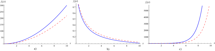
Fig. 1.: Behavior of the usual derivative $d/dx$ (solid line) with $\mu=0$ and its $\mu$-deformed analog $\mathcal{D}^{(\mu)}_{x}$ (dashed line) with $\mu=0.7$ acting on $f_{1}=x^{3}$, $f_{2}=\ln(1+x)$, and $f_{3}=\exp(x)$: (a), (b), and (c), respectively

This fact may serve to partly justify  the use of the $\mu$-derivative, instead of the ordinary one, in calculating some thermodynamical quantities in the $\mu$-Bose gas model. Then, through the use of the $\mu$-analog of the derivative, the deformation parameter gets involved in the treatment, and, thus, the whole system is $\mu$-deformed.

It is important that, with the use of the $\mu$-bracket $[n]_{\mu}$ and the $\mu$-factorial $[n]_{\mu}!$ given in (7) and (9), respectively, we can consider the $\mu$-deformed analogs of elementary functions such as, e.g., the $\mu$-exponential function $\exp_{\mu}(x)$,

$$\exp_{\mu}(x)\!=\!\sum_{n=0}^{\infty}\frac{x^{n}}{[n]_{\mu}!},$$

or the $\mu$-logarithmic function $\ln_{\mu}(x)$,

$$\ln_{\mu}(x)=-\sum_{n=1}^{\infty}\frac{(1-x)^{n}}{[n]_{\mu}}.$$

The $\mu$-number $[n]_{\mu}$ and the $\mu$-factorial $[n]_{\mu}!$ reduce, as $\mu\rightarrow 0,$ to $n$ and $n!$, and we recover the usual exponential and logarithmic functions.

In Figs. 2 and 3, the $\mu$-deformed analogs of the exponential and logarithmic functions are shown. It is clear that some special functions (e.g., the $\mu$-analog of polylogarithms, see below) can also appear.

Let us introduce the $\mu$-analog ($\mu$-polylogarithm) of the well-known Bose function or polylogarithm $g_{l}(z)=$ $=\sum_{n=1}^{\infty}z^{n}/n^{l}$, namely:

$$g_{l}^{(\mu)}(z)=\sum_{n=1}^{\infty}\frac{[n]_{\mu}}{n^{l+1}}z^{n}.$$ (10)

Its simplest special case is the function $g_{0}^{(\mu)}(z)=$ $=\sum_{n=1}^{\infty}\frac{[n]_{\mu}}{n}z^{n}\stackrel{{\scriptstyle\mu=0}}{{\longrightarrow}}\sum_{n=1}^{\infty}z^{n}$. Clearly, it reduces to $\ln(1-z)$ if $\mu=0$. In Fig. 4, we illustrate the dependence of the deformed Bose functions $g_{0}^{\mu}$, $g_{1}^{\mu}$, $g_{2}^{\mu}$, and $g_{5}^{\mu}$ on the fugacity $z$ at $\mu=0.4$.

$\mu$-Derivative $D^{(\mu)}_{x}$​
and $\mu$-analog of the Leibnitz rule

Consider how the $\mu$-differentiation acts upon the product $f(x)g(x)$ of two functions. In the simple case of monomials $f(x)=x^{n}$ and $g(x)=x^{m},$ we have

$$D^{(\mu)}_{x}\left(x^{n}x^{m}\right)=D^{(\mu)}_{x}\left(x^{m}x^{n}\right)=$$

$$=\frac{n+m}{1+\mu(n+m)}\,x^{n+m-1}.$$ (11)

More involved is the case of general functions,

$$D^{(\mu)}_{x}\left(f(x)g(x)\right)=\int\limits^{1}_{0}[f(t^{\mu}x)g(t^{\mu}x)]^{\prime}_{x}{\rm d}t=\mbox{...}.$$ (12)

which After the integration by parts, we obtain

$$D^{(\mu)}_{x}\left(f(x)g(x)\right)=g(x)D^{(\mu)}_{x}f(x)+f(x)D^{(\mu)}_{x}g(x)-$$

$$-\Bigl{(}g(0)D^{(\mu)}_{x}f(x)+f(0)D^{(\mu)}_{x}g(x)\Bigr{)}-$$

$$-\int\limits_{0}^{1}{\rm d}t\left[g^{\prime}_{t}(xt^{\mu})\Bigl{(}\int{\rm d}sf^{\prime}_{x}(xs^{\mu})\Bigr{)}_{s\to t}\,+\right.$$

$$\left.+\,f^{\prime}_{t}(xt^{\mu})\Bigl{(}\int{\rm d}sg^{\prime}_{x}(xs^{\mu})\Bigr{)}_{s\to t}\right]\!.$$

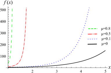
Fig. 2.: $\mu$-Deformed analog of the exponential function: $f(x)=\exp_{\mu}(x)$

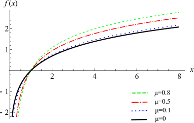
Fig. 3.: $\mu$-Deformed analogs of the logarithmic function. Here, $f(x)=\ln_{\mu}(x)$

Note that, for the functions with the property $g(0)=$ $=0$ and $f(0)=0$, this general formula somewhat simplifies. In the particular case of a product of monomials, the above formula (11) is recovered.

3 Different Ways
to Deform the Bose Gas Model

As known, the system of standard oscillators (bosons) as an idealized model may be rather far from real physical systems. Say, in case of a standard harmonic oscillator, the interaction is ignored.

Here, like many other papers studying deformed oscillators (e.g., [13,​ 15,​ 24]), we consider a many-body system of deformed bosons or deformed oscillators. One of the virtues of a deformation is the ability to effectively account for the interaction between particles [13,​ 14], their non-zero volume [25], or their inner structure (composite nature) [26]. The joint account of two of these factors is also possible [27].

A special deformed Bose gas model that is the $\mu$-Bose gas model associated with $\mu$-deformed oscillators [12] was introduced and studied in [6,​ 28]. Therein, the main concern was the calculation of correlation functions and their intercepts. In [16], the study of the thermodynamics of a $\mu$-Bose gas has begun.

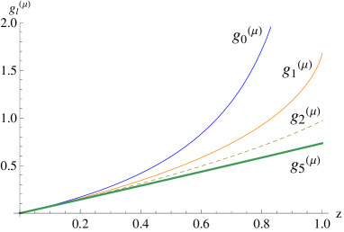
Fig. 4.: Dependence of the functions $g_{0}^{\mu}$, $g_{1}^{\mu}$, $g_{2}^{\mu}$, and $g_{5}^{\mu}$ on the fugacity $z=\exp(\beta\widetilde{\mu})$ at $\mu=0.4$

For the thermal average of an operator $\mathcal{O},$ we use the formula (that for the Hamiltonian is given below)

$$\langle\mathcal{O}\rangle=\frac{Tr(\mathcal{O}e^{-\beta H})}{Z},$$ (13)

with $Z$ being the grand canonical partition function. Its logarithm in the non-deformed case is

$$\ln Z=-\sum_{i}\ln(1-ze^{-\beta\varepsilon_{i}})$$ (14)

with the fugacity $z=e^{\beta\widetilde{\mu}}$. The total number of  par-

ticles is calculated from the formula

$$N=z\frac{d}{dz}\ln Z,$$

which will be modified for the purposes of the present treatment (see the next section for the $\mu$-defor- med case).

For deformed oscillators and a $\mu$-deformed Bose gas, the deformation parameter is inevitably present. Note that the building of a deformed analog of the Bose gas model can be done in different ways:

– By taking a modified/deformed Hamiltonian for the system:

$$H=\sum_{i}(\varepsilon_{i}-\widetilde{\mu})[N_{i}],$$ (15)

where $\varepsilon_{i}$ is the kinetic energy of particles, $\widetilde{\mu}$ is the chemical potential, and $[X]\neq X$ stands for the deformed bracket.

– By proceeding with the usual Hamiltonian $H=$$=\sum_{i}(\varepsilon_{i}-\widetilde{\mu})N_{i}$ and then using the (technique of) modified calculus.  Namely, instead of the usual derivative, one uses some its generalization to obtain thermodynamical functions. Then all thermodynamical functions will depend on the deformation parameter.

– Here, we perceive another, specially designed way. Namely, we use the generalized derivative only once: to obtain the expression for the total number of particle; then we use this result to get the deformed partition function. Having derived the $\mu$-deformed partition function, we easily find all the other (also deformed) thermodynamical functions.

4 $\mu$-Deformation of the Bose Gas Model: Correlation Functions

The system of standard oscillators or bosons, as an idealized model, usually is very distant from real physical systems. As known, the standard harmonic oscillator implies the absence of interaction.

In our treatment, like many other papers studying the deformed oscillators (see, e.g., [24,​ 14,​ 15]), we consider a set of deformed oscillators or deformed bosons. Concerning the deformed models, let us stress its ability to effectively account for the interaction between particles; their non-zero volume; and their inner structure or composite nature.

The $\mu$-deformed analog of the Bose gas model ($\mu$-Bose gas) is the model describing the many-particle system of $\mu$-deformed bosons with the Hamiltonian 

$$H=\sum_{i}(\varepsilon_{i}-\widetilde{\mu})N_{i},$$ (16)

which is similar to the case of ordinary bosons (the simplest possible form). Here, $\varepsilon_{i}$ in (16) denotes the kinetic energy of a particle in the state ‘‘$i$’’, $N_{i}$ is the particle number (occupation number) operator corresponding to the state ‘‘$i$’’. The thermodynamic study of the new model will be based on special mathematical techniques – the so-called $\mu$-calculus described above.

The $\mu$-Bose gas model associated with $\mu$-deformed oscillators [12] was first introduced and studied in [6]. This model has a potential for the explanation of the non-Bose like behavior of the intercepts of the momentum correlation functions of real particles such as $\pi$-mesons. Some further development of the correlation function (and intercept) aspects of the $\mu$-Bose gas model was made in [28]. Note that, due to these efforts, the intercepts of the second, third and higher order correlation functions are known in explicit analytic form.

5 Thermodynamic Functions
of the $\mu$-Bose Gas Model

We now study the thermodynamics (see [16]) of the $\mu$-deformed analog of a Bose gas in more details, by using the $\mu$-calculus given above. We consider non-relativistic particles. Below, the regimes of high and low temperatures will be considered. First of all, let us calculate the total number of particles.

Total number of particles

As mentioned, the relation giving the total number of particles in the Bose gas model is

$$N=z\frac{d}{dz}\ln Z.$$ (17)

To deal with the thermodynamics of a $\mu$-deformed analog of the Bose gas model, formula (17) for the total number $N$ should be modified. Namely, we take

$$N^{(\mu)}=z\mathcal{D}^{(\mu)}_{z}\ln Z=-z\mathcal{D}^{(\mu)}_{z}\sum_{i}\ln(1-ze^{-\beta\varepsilon_{i}}),$$ (18)

where $\mathcal{D}^{(\mu)}$ is the $\mu$-derivative from (7).

We apply this, assuming $0\leq\mu<1$, to the logarithm of the partition function in (14) to get

$$N^{(\mu)}=z\sum_{i}\sum_{n=1}^{\infty}\frac{(e^{-\beta\varepsilon_{i}})^{n}}{n}[n]_{\mu}z^{n-1}=$$

$$=\sum_{i}\sum_{n=1}^{\infty}\frac{[n]_{\mu}}{n}(e^{-\beta\varepsilon_{i}})^{n}z^{n}.$$ (19)

For consistency, we require $0\leq|ze^{-\beta\varepsilon_{i}}|<1$ in (19). Since non-relativistic particles are considered, the energy of the $i$-th particle of the system is

$$\varepsilon_{i}=\frac{{\bf p}_{i}{\bf p}_{i}}{2m}=\frac{|p|^{2}}{2m}=\frac{p_{i}^{2}}{2m},$$ (20)

where ${\bf p}_{i}$ the 3-momentum of the particle in the $i$-th state, and $m$ is particle’s mass.

As seen, as $z\rightarrow 1,$ the expression in the summand in (19) diverges when $p_{i}=0,i=0$. Below, we assume the $i=0$ ground state is associated with a macroscopically large occupation number. Then, even though $z\neq 1$, we separate the term with $p_{i}=0$ from the remaining sum:

$$N^{(\mu)}={\sum_{i}}^{\prime}\sum_{n=1}^{\infty}\frac{[n]_{\mu}}{n}(e^{-\beta\varepsilon_{i}})^{n}z^{n}+\sum_{n=1}^{\infty}\frac{[n]_{\mu}}{n}z^{n}.$$ (21)

The ‘‘prime’’ marking the outer sum in (21) means that the $i=0$ term is dropped from the sum. For large volumes $V$ and large $N$, the spectrum of single-particle states is almost a continuous one, and we replace the sum in (19) by the integral:

$$\sum_{i}\rightarrow\frac{V}{(2\pi\hbar)^{3}}\int d^{3}k.$$

In other words, we isolate the ground state, and the contribution from all the other states is included in the integral. WE now perform the integration over 3-momenta using spherical coordinates:

$$N^{(\mu)}=\frac{4\pi V}{(2\pi\hbar^{2})^{3}}\sum_{n=1}^{\infty}\frac{[n]_{\mu}}{n}z^{n}\times$$

$$\times\int\limits^{\infty}_{0}p^{2}e^{-\beta p^{2}/2m}dp+\sum_{n=1}^{\infty}\frac{[n]_{\mu}}{n}z^{n}.$$ (22)

The lower limit of the integral can still be taken as zero, because the ground state, $p_{0}$, does not contribute to the integral anyway. By performing the integration, we finally obtain that the ($\mu$-deformed, i.e., depending on $\mu$) total number of particles is given by the expression

$$N^{(\mu)}\!=\!\frac{V}{\lambda^{3}}\sum_{n=1}^{\infty}\!\frac{[n]_{\mu}}{n^{5/2}}z^{n}\!+\!N_{0}^{(\mu)},\leavevmode\nobreak\ \leavevmode\nobreak\ N_{0}^{(\mu)}\!\equiv\!\sum_{n=1}^{\infty}\!\frac{[n]_{\mu}}{n}z^{n},$$ (23)

which will be used for deriving the $\mu$-partition function.

Deformed partition function,
equation of state

Let all the known relations between thermodynamical quantities known in case of the usual Bose gas thermodynamics be promoted to its $\mu$-deformed analog. That is, the well-known relations for the usual Bose gas model and its $\mu$-deformed counterpart are formally similar. However, all the thermodynamical quantities for the $\mu$-Bose gas model become $\mu$-dependent.

To obtain the $\mu$-partition function $\ln Z^{(\mu)}$ from

$$N^{(\mu)}=z\frac{d}{dz}\ln Z^{(\mu)},$$ (24)

we invert it:

$$\ln Z^{(\mu)}=\bigg{(}\!z\frac{d}{dz}\!\bigg{)}^{\!-1}N^{(\mu)}.$$ (25)

To perform the operation $\bigl{(}z\frac{d}{dz}\bigr{)}^{-1}$ and to get $\ln Z^{(\mu)}$, we may either integrate $\ln Z^{(\mu)}=\int\!dz\leavevmode\nobreak\ z^{-1}N^{(\mu)}$ or, equivalently, apply the following property valid on the monomials $z^{k}$ for any function $f(z\frac{d}{dz})$ possessing a power series expansion:

$$f\bigg{(}\!z\frac{d}{dz}\!\bigg{)}z^{k}=f(k)z^{k}.$$ (26)

In view of this, relations (25) and (21)–(23) yield

$$\ln Z^{(\mu)}=\bigg{(}\!z\frac{d}{dz}\!\bigg{)}^{\!-1}\!\left(\!\frac{V}{\lambda^{3}}\sum_{n=1}^{\infty}\frac{[n]_{\mu}}{n^{5/2}}z^{n}+\sum_{n=1}^{\infty}\frac{[n]_{\mu}}{n}z^{n}\!\right)\!=$$

$$=\frac{V}{\lambda^{3}}\sum_{n=1}^{\infty}\frac{[n]_{\mu}}{n^{5/2}}\bigg{(}\!z\frac{d}{dz}\bigg{)}^{\!-1}z^{n}+\sum_{n=1}^{\infty}\frac{[n]_{\mu}}{n}\bigg{(}\!z\frac{d}{dz}\bigg{)}^{\!-1}z^{n}=$$

$$=\frac{V}{\lambda^{3}}\sum_{n=1}^{\infty}\frac{[n]_{\mu}}{n^{5/2}}(n)^{-1}z^{n}+\sum_{n=1}^{\infty}\frac{[n]_{\mu}}{n}(n)^{-1}z^{n}.$$ (27)

The latter result can be written as (see (10))

$$\ln Z^{(\mu)}=\frac{V}{\lambda^{3}}g^{(\mu)}_{5/2}+g^{(\mu)}_{1}$$ (28)

or, equivalently, as

$$Z^{(\mu)}(z,T,V)=\exp\left(\!\frac{V}{\lambda^{3}}g^{(\mu)}_{5/2}(z)+g^{(\mu)}_{1}(z)\!\right)\!.$$ (29)

Formulas (27)–(29) for the $\mu$-deformed partition function constitute our main result. Using (29), it is now possible to derive other thermodynamical functions. The equation of state reads

$$\frac{PV}{kT}=\ln Z^{(\mu)}=\frac{V}{\lambda^{3}}g^{(\mu)}_{5/2}(z)+g^{(\mu)}_{1}(z).$$ (30)

Remark that an alternative way of obtaining the $\mu$-deformed partition function could be the use of the one-particle $\mu$-deformed distribution function $\langle n\rangle^{(\mu)}$ found in analytical form in [28]. Note that the result derived in such way will slightly differ from that given in (29). The details will be given elsewhere.

Virial expansion and virial coefficients

Let us consider the physical meaning of the parameter $\mu$. In the case of ideal Bose gas, the virial coefficients are responsible for the effective (two-particle, three-particle, etc.) interactions of the quantum-correlation or quantum-statistical origin. In a $\mu$-Bose gas, the inner structure/compositeness of particles or interactions between them are effectively taken into account (like other deformations of the Bose gas model) by means of the involved parameter $\mu$. Clearly, this results in an additional effective interaction (revealed by the deformed virial coefficients).

Consider the regime of high temperature and low density $\lambda^{3}/v\ll 1$. As explained, e.g., in [29], the second term in (23) in this case is negligibly small. This is also true for Eq. (30). Expression (23) and the equation of state (30) take the form

$$\frac{\lambda^{3}}{v}=g^{(\mu)}_{3/2}(z),\quad\frac{Pv}{kT}=\frac{v}{\lambda^{3}}g^{(\mu)}_{5/2}(z),$$ (31)

respectively. From the first relation in (31), we have

$$\frac{\lambda^{3}}{v}=z+\frac{[2]_{\mu}}{2^{5/2}}z^{2}+\frac{[3]_{\mu}}{3^{5/2}}z^{3}+\frac{[4]_{\mu}}{4^{5/2}}z^{4}+\frac{[5]_{\mu}}{5^{5/2}}z^{5}+...,$$ (32)

$[k]_{\mu}$ being the $\mu$-number corresponding to $k$. Inverting the series in (32), we derive the virial expansion for the equation of state

$$\frac{Pv}{kT}=1+A\bigg{(}\!\frac{\lambda^{3}}{v}\!\bigg{)}+B\bigg{(}\!\frac{\lambda^{3}}{v}\bigg{)}^{\!2}+C\bigg{(}\!\frac{\lambda^{3}}{v}\!\bigg{)}^{\!3}+D\bigg{(}\!\frac{\lambda^{3}}{v}\!\bigg{)}^{\!4}\!+...,$$ (33)

where the second to fifth virial coefficients are:

$$A=-\frac{[2]_{\mu}}{2^{7/2}[1]^{2}_{\mu}},\quad B=\frac{[2]_{\mu}^{2}}{2^{5}[1]_{\mu}^{4}}-\frac{2[3]_{\mu}}{3^{7/2}[1]_{\mu}^{3}},$$

$$C=-\frac{5[2]^{3}_{\mu}}{2^{17/2}[1]^{6}_{\mu}}+\frac{[2]_{\mu}[3]_{\mu}}{2^{5/2}3^{3/2}[1]^{5}_{\mu}}-\frac{3[4]_{\mu}}{2^{7}[1]^{4}_{\mu}},$$

$$D\!=\!\frac{7[2]^{4}_{\mu}}{2^{10}[1]^{8}_{\mu}}-\frac{[2]^{2}_{\mu}[3]_{\mu}}{2^{3}3^{3/2}[1]^{7}_{\mu}}+\frac{2[3]^{2}_{\mu}}{3^{5}[1]^{6}_{\mu}}+\frac{[2]_{\mu}[4]_{\mu}}{2^{11/2}[1]^{6}_{\mu}}-\frac{4[5]_{\mu}}{5^{7/2}[1]^{5}_{\mu}}.$$ (34)

The deformation parameter $\mu$ appears in the expressions for virial coefficients in a specific manner, only through the $\mu$-bracket of integers. We encounter a very unusual feature: the appearance of the (powers of) $\mu$-unity $[1]_{\mu}$. Note that its analog was absent in the virial coefficients for the cases of a $q$-Bose or $p,q$-Bose gas because of the equality $[1]_{p,q}=1$, see [30]. In the case at hands due to $[1]_{\mu}=\frac{1}{1+\mu}\neq 1,$ the $\mu$-deformed virial coefficients contain $[1]_{\mu}$ squared and also higher powers of $\mu$-unity.

Remark. By changing the value of deformation parameter, one can regulate not only the magnitude, but also the sign of virial coefficient(s) and, thus, even can get a repulsive instead of attractive (or vice versa) effective interparticle interaction in a model system. Generally speaking, by driving the value of $\mu,$ we can effectively change (control) the very quantum statistics of particles, compare with [14,​ 31,​ 32].

Internal energy, specific heat,
and entropy at $T>T_{c}^{(\mu)}$

For a deformed analog of the Bose gas model we adopt the known definition of thermodynamical functions [33]. The internal energy $U^{(\mu)}$ of a $\mu$-Bose gas is then found as $U^{(\mu)}=-\left(\!\partial\ln Z^{(\mu)}/\partial\beta\!\right)_{z,V}$. First, we examine the case $T>T_{c}^{(\mu)}$:

$$\frac{U^{(\mu)}}{N^{(\mu)}}=\frac{3}{2}\frac{kTv}{\lambda^{3}}g^{(\mu)}_{5/2}(z),\quad T>T_{c}^{(\mu)}.$$ (35)

From the expressions for the internal energy of a $\mu$-Bose gas, we obtain the specific heat of the system, using the relation $C_{v}=\left(\partial U/\partial T\right)_{N,V}$. The result is

$$\frac{C_{v}^{(\mu)}}{N^{(\mu)}k}\!=\!\frac{15}{4}\frac{v}{\lambda^{3}}g^{(\mu)}_{5/2}(z)-\frac{9}{4}\frac{g^{(\mu)}_{3/2}{(z)}}{g^{(\mu)}_{1/2}{(z)}},\quad T>T_{c}^{(\mu)}.$$ (36)

Note that, both in (35) and (36), the $\mu$-deformed analog (or $\mu$-polylogarithm) of the Bose function $g_{n}(z)$ does appear. This fact may have interesting implications.

The formula for the entropy, $S=\ln Z+\beta U-\beta\widetilde{\mu}N,$ for the $\mu$-analog of a Bose gas in the regime of high temperature reads

$$\frac{S^{(\mu)}}{N^{(\mu)}k}=\frac{5}{2}\frac{V}{\lambda^{3}}g^{(\mu)}_{5/2}(z)-\ln z,\quad T>T^{(\mu)}_{c}.$$ (37)

It will be interesting to explore the obtained formulas in different related contexts, and this is postponed for a subsequent report.

Critical temperature of condensation
and other thermodynamical functions

In the regime of low temperature and high density, let us obtain (say, like in [30] for the case of the $p,q$-Bose gas model) the critical temperature $T^{(\mu)}_{c}$ of the considered $\mu$-analog of the Bose gas model. We start with Eq. (23) and rewrite it as

$$\frac{N_{0}^{(\mu)}}{V}=\frac{\lambda^{3}}{v}-g^{(\mu)}_{3/2}(z).$$ (38)

The critical temperature $T_{c}^{(\mu)}$ of a $\mu$-Bose gas is determined from the equation $\lambda^{3}/{v}=g^{(\mu)}_{3/2}(1)$:

$$T_{c}^{(\mu)}=\frac{2\pi\hbar^{2}/mk}{\bigl{(}vg^{(\mu)}_{3/2}(1)\bigr{)}^{2/3}}.$$ (39)

From this, we infer the ratio of the critical temperature $T_{c}^{(\mu)}$ to the usual Bose gas critical temperature $T_{c}$:

$$\frac{T_{c}^{(\mu)}}{T_{c}}=\Biggl{(}\frac{2.61}{g^{(\mu)}_{3/2}(1)}\!\Biggr{)}^{\!\!2/3}\!.$$ (40)

Figure 5 shows how the obtained ratio (40) depends on the parameter $\mu$ (i.e., on the deformation strength).

Observe that, similarly to the case of a $p,q$-analog of the Bose gas model (see [30]), the ratio $\frac{T_{c}^{(\mu)}}{T_{c}}$ has the important characteristic feature: the greater the deformation strength (here given by $\mu$), the higher is $T_{c}^{(\mu)}$. In the no-deformation limit $\mu\rightarrow 0,$ we have $T_{c}^{(\mu)}/{T_{c}}=1$. That is, as $\mu\rightarrow 0$, the $\mu$-critical temperature goes over into the usual one, $T_{c}^{(\mu)}\rightarrow T_{c}$ (a kind of consistency). If we drive the deformation strength, we could raise the critical temperature significantly.

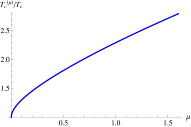
Fig. 5.: Dependence of the ratio $T_{c}^{(\mu)}/{T_{c}}$ on the $\mu$-parameter

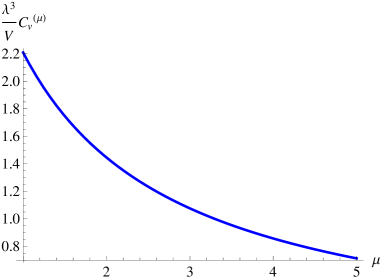
Fig. 6.: Dependence of the specific heat $C_{v}^{(\mu)}$ (multiplied by $\frac{\lambda^{3}}{V}$) on the deformation parameter $\mu$

Now, we present the expressions for some thermodynamical functions, again for low temperatures. It is easy to obtain the internal energy

$$\frac{U^{(\mu)}}{N^{(\mu)}}=\frac{3}{2}\frac{kTv}{\lambda^{3}}g^{(\mu)}_{5/2}(1),\quad T\leq T_{c}^{(\mu)},$$ (41)

the specific heat

$$\frac{C_{v}^{(\mu)}}{N^{(\mu)}k}=\frac{15}{4}\frac{v}{\lambda^{3}}g^{(\mu)}_{5/2}(1),\quad T\leq T_{c}^{(\mu)},$$ (42)

and the expression for the entropy (at $T\leq T_{c}^{(\mu)}$):

$$\frac{S^{(\mu)}}{N^{(\mu)}k}=\frac{5}{2}\frac{V}{\lambda^{3}}g^{(\mu)}_{5/2}(1),\quad T\leq T^{(\mu)}_{c}.$$ (43)

In Fig. 6, the dependence of the specific heat on the parameter $\mu$ (deformation strength) is shown.

6 Discussion, Outlook

For the $\mu$-analog of the Bose gas model proposed and studied earlier to some extent, we have explored a number of main thermodynamical functions or relations. After presenting and discussing the necessary elements of the $\mu$-calculus based on the use of the $\mu$-deformed analog of the usual derivative, we have explicitly derived the expression for the total mean number of particles. This important result allowed us to obtain the $\mu$-deformed partition function as well. As a result, we have got via the $\mu$-derivative that the deformation parameter has entered the expressions for the total number of particles and the partition function. While the $\mu$-deformed analog $g^{(\mu)}_{3/2}(z)$ of the polylogarithms $g_{n}(z)$ becomes involved in the formula for $N^{(\mu)}$, the $\mu$-polylogarithm $g^{(\mu)}_{5/2}(z)$ has naturally appeared in the $\mu$-partition function.

Analyzing the high-temperature regime, we have obtained explicitly the virial expansion for the equation of state along with the first five virial coefficients. The deformation parameter $\mu$ enters the expressions for virial coefficients through the $\mu$-bracket of integers. Since the deformed system at $\mu\neq 0$ basically differs from the bosonic one, it is obvious that a small variation of $\mu$ changes smoothly the statistics of particles. Moreover, by governing the value of $\mu$, we are able to achieve such drastic change as switching of the sign of virial coefficient(s), that implies the basic change of the type of statistics. As it is obligatory for consistency, one can easily verify that, in the no-deformation limit $\mu=0,$ the known virial coefficients of the usual Bose gas are reproduced from the just obtained $\mu$-deformed virial coefficients.

In the low temperature regime, the critical temperature (as a function of $\mu$) of the analog of Bose condensation is obtained. The dependence of the ratio $T_{c}^{(\mu)}/{T_{c}}$ on the deformation parameter $\mu$ shows that the critical temperature of a $\mu$-Bose gas is higher than $T_{c}$ of the usual Bose gas. This fact can be obviously viewed as interesting and very useful for the goals of the future more elaborated investigation of real Bose-like gases, in parallel to a similar use of the result for the critical temperature $T_{c}^{(p,q)}$ of the $p,q$-Bose gas model. Elsewhere, we hope to draw some interesting consequences of our formulas for $C^{(\mu)}_{v}$ and $S^{(\mu)}$.

This work was partly supported by the Special Program of the Division of Physics and Astronomy of the NAS of Ukraine and (A.P.R.) by the Grant for Young Scientists of the NAS of Ukraine (No. 0113U004910).

А.П. Ребеш, I.I. Качурик, О.М. Гаврилик
ЕЛЕМЕНТИ $\mu$-ЧИСЛЕННЯ
ТА ТЕРМОДИНАМIКА МОДЕЛI $\mu$-БОЗЕ-ГАЗУ
Р е з ю м е
На основi $\mu$-деформованих осциляторiв розроблено деформований аналог моделi бозе-газу ($\mu$-бозе-газ). В рамках нової моделi в режимi низьких температур ми отримали вiрiальний розклад рiвняння стану, а також першi п’ять вiрiальних коефiцiєнтiв; в режимi низьких температур обчислено критичну температуру конденсацiї. Ми також отримали питому теплоємнiсть, внутрiшню енергiю та ентропiю для $\mu$-бозе-газу у випадках низьких та високих температур. Усi термодинамiчнi функцiї виявилися залежними вiд параметра деформацiї. Дослiджено залежнiсть питомої теплоємностi вiд параметра деформацiї.

References

- [1] O.W. Greenberg, Phys. Rev. Lett. 64, 705 (1990).
- [2] F. Wilczek, Phys. Rev. Lett. 49, 957 (1982).
- [3] Y.-H. Chen, F. Wilczek, E. Witten, and B. Halperin, Int. J. Mod. Phys. B. 3, 1001 (1989).
- [4] D.V. Anchishkin, A.M. Gavrilik, and S.Y. Panitkin, Ukr. Phys. J. 49, 935 (2004).
- [5] A.M. Gavrilik, SIGMA 2, 074 (2006).
- [6] A. Gavrilik and A. Rebesh, Eur. Phys. J. A 47, 55 (2011).
- [7] T. Kobayashi and T. Suzuki, J. Phys. A. 26, 6055 (1993).
- [8] M. Arik and D.D. Coon, J. Math. Phys. 17, 524 (1976).
- [9] L.C. Biedenharn, J. Phys. A: Math. Gen. 22, L873 (1989).
- [10] A.J. Macfarlane, J. Phys. A: Math. Gen. 22, 4581 (1989).
- [11] A. Chakrabarti and R. Jagannathan, J. Phys. A: Math. Gen. 24, L711 (1991).
- [12] A. Jannussis, J. Phys. A: Math. Gen. 26, L233 (1993).
- [13] A.M. Scarfone and P. Narayana Swamy, J. Phys. A: Math. Theor. 41, 275211 (2012).
- [14] A.M. Scarfone and P. Narayana Swamy, J. Stat. Mech. 2009, 02055 (2009).
- [15] A. Algin, Commun. Nonlinear Sci. Numer. Simulat. 15, 1372 (2010).
- [16] A.M. Gavrilik and A.P. Rebesh, ArXiv: 1309.1363 [cond-mat.stat-mech].
- [17] F. Jackson, Trans. Royal. Soc. Edinb. 46, 253 (1908).
- [18] A. Erzan and A. Gorbon, Turk. J. of Phys. 23, 9 (1999).
- [19] A.M. Gavrilik and A.P. Rebesh, J. Phys. A: Math. Theor. 43, 095203 (2010).
- [20] V. Kac and P. Cheung, Quantum Calculus (Springer, Berlin, 2002).
- [21] R.A. Floreanini, J. Phys. A 26, L611 (1993).
- [22] I.M. Burban and A.U. Klimyk, Integr. Transf. Spec. Funct. 2, 15 (1994).
- [23] A.M. Gavrilik, I.I. Kachurik, and A.P. Rebesh, J. Phys. A: Math. Theor. 43, 245204 (2010).
- [24] M. Rego-Monteiro, L.M.C.S. Rodrigues, and S. Wulck, Phys. Rev. Lett. 76, 1098 (1996).
- [25] S.S. Avancini and G. Krein, J. Phys. A: Math. Gen. 28, 685 (1995).
- [26] A.M. Gavrilik, I.I. Kachurik, and Yu.A. Mishchenko, J. Phys. A: Math. Theor. 58, 1172 (2013).
- [27] A.M. Gavrilik and Yu.A. Mishchenko, Ukr. Phys. J. 49, 935 (2013).
- [28] A.M. Gavrilik and Yu.A. Mishchenko, Phys. Lett. A 376, 2484 (2012).
- [29] K. Huang, Statistical Mechanics (Wiley, New York, 1987).
- [30] A.M. Gavrilik and A.P. Rebesh, Mod. Phys. Lett. B 26, 1150030 (2012).
- [31] A. Algin and M. Senay, Phys. Rev. E 85, 041123 (2012).
- [32] M. Ubriaco, Phys. Lett. A 376, 3581 (2012).
-
[33]
R.K. Pathria and P.D. Beale, Statistical Mechanics (Elsevier, Amsterdam, 2011).
Received 24.09.13