Application of the parallel multicanonical method to lattice gas condensation

Abstract

We present the speedup from a novel parallel implementation of the multicanonical method on the example of a lattice gas in two and three dimensions. In this approach, all cores perform independent equilibrium runs with identical weights, collecting their sampled histograms after each iteration in order to estimate consecutive weights. The weights are then redistributed to all cores. These steps are repeated until the weights are converged. This procedure benefits from a minimum of communication while distributing the necessary amount of statistics efficiently.

Using this method allows us to study a broad temperature range for a variety of large and complex systems. Here, a gas is modeled as particles on the lattice, which interact only with their nearest neighbors. For a fixed density this model is equivalent to the Ising model with fixed magnetization. We compare our results to an analytic prediction for equilibrium droplet formation, confirming that a single macroscopic droplet forms only above a critical density.

1 Introduction

Despite the large amount of existing literature, condensation remains under investigation up to today by means of analytical treatment, numerical studies, and experiments  [1, 2, 3, 4, 5, 6, 7, 8]. In addition to the increasing interest in non-equilibrium properties and droplet size distributions, questions regarding the equilibrium properties remain open as well. For example, Biskup et al. [3, 4] showed that in equilibrium an over-saturated gas system is either in the evaporated phase or in the condensed phase consisting of a single macroscopic droplet. The probability for droplets of intermediate size is negligibly small. This result was proven for the two-dimensional Ising model and numerically verified [7, 8]. We set out to test this analytical result also for the three-dimensional case of a lattice gas. Due to the nucleation barrier, we applied a parallel implementation [9] (for related methods see [10, 11, 12]) of multicanonical simulations [13, 14, 15] to circumvent a possible hysteresis, driving the system back and forth between the condensed and evaporated phase.

We start by describing the main method and the theoretical arguments together with the model. This is followed by a comparison to micromagnetic simulations of the equivalent Ising model in order to verify the correctness. We discuss the speedup with increasing parallelization and compare the simulation effort with the independent micromagnetic simulation. Afterwards, the results in two and three dimensions are presented and discussed, followed by some concluding remarks.

2 Method

The multicanonical method [13, 14, 15] enables the sampling of a broad parameter space in a single simulation by modifying the acceptance probability according to a simple idea. The Boltzmann factor is replaced, or sometimes extended, by a weight function with the purpose to increase the probability to reach states that are suppressed otherwise. This can be achieved for a variety of order parameters leading to multimagnetic, multibondic and many more realizations but can best be explained for the case of the internal energy $E$. Formally, this can be described by writing the partition function in terms of the density of states $\Omega(E)$,

$$Z_{\rm can}=\sum_{E}\Omega(E)e^{-\beta E}\rightarrow\sum_{E}\Omega(E)W(E),$$ (1)

where we have already transformed the Boltzmann factor into the weight function $W(E)$. Analogous to the Metropolis algorithm, new states ($E_{n}$) are generated from old states ($E_{o}$) and accepted with

$$\min\left(1,\frac{W(E_{n})}{W(E_{o})}\right).$$

If we were to know $\Omega(E)$, we could sample the full energy range with a flat distribution choosing $W(E)=1/\Omega(E)$. However, this is in general not the case such that $W(E)$ has to be obtained in an iterative way. This can be simple or complex; it can modify the weights on the fly or rely on equilibrium distributions in each iteration. A simple example would be to perform equilibrium simulations with initial weights $W^{i}$ and estimate the consecutive weights as $W^{i+1}(E)=W^{i}(E)/H^{i}(E)$. Hence, if a state occurs more often the weight is reduced more strongly.

We applied a parallel version of this multicanonical method which has been shown to exhibit an ideal scaling for the Ising model and a very good scaling for the $q=8$ Potts model [9]. This parallel implementation relies on equilibrium iterations, distributing the sampling of the distribution $H^{i}(E)$ on $p$ independent processes. Since the weights are not modified within a single iteration, each process returns a contribution to the same distribution and they can simply be summed up:

$$H^{i}(E)=\sum_{j=1}^{p}H^{i}_{j}(E)$$ (2)

Afterwards, the consecutive weights are calculated from the previous weights together with the total histogram according to whatever rule one may choose, in our case by a recursive scheme [15].

Altogether, this leads to an efficient parallelization due to a very limited amount of communication. Below, we will show the applicability of the method to a general problem, here the condensation of a lattice gas in two and three dimensions. As in real life and other than in [9], we will not pay attention to the optimization of each degree of parallelization but want to demonstrate the value of this parallelization to modern computational statistical physics.

3 Condensation of a lattice gas

A general theory of equilibrium droplet condensation was proposed by Biskup et al. [3, 4], with a rigorous analytic solution for the two-dimensional Ising spin model. In principle they describe the interplay of entropy maximization by vacuum fluctuations with energy minimization by forming a droplet. They showed that the probability for intermediate-size droplets vanishes with increasing system size. The free energy consists of a contribution from the vacuum fluctuation of excess particles $\delta N$

$$F_{\rm fluc}=\frac{(\delta N)^{2}}{2\hat{\kappa}V},$$ (3)

with the isothermal compressibility $\hat{\kappa}=\beta\kappa=\beta\left\langle\left(N-\langle N\rangle\right)^{2}\right\rangle/V$ and a contribution from the single largest droplet of size $V_{D}$

$$F_{\rm drop}=\tau_{W}(V_{D})^{\frac{d-1}{d}},$$ (4)

where $\tau_{W}$ is the surface free energy of a (Wulff shaped) droplet of unit volume (see Fig. 1).

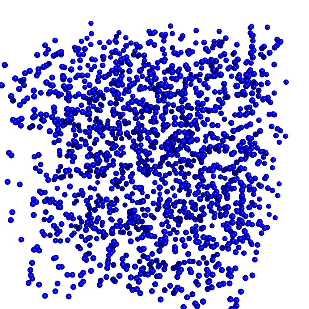
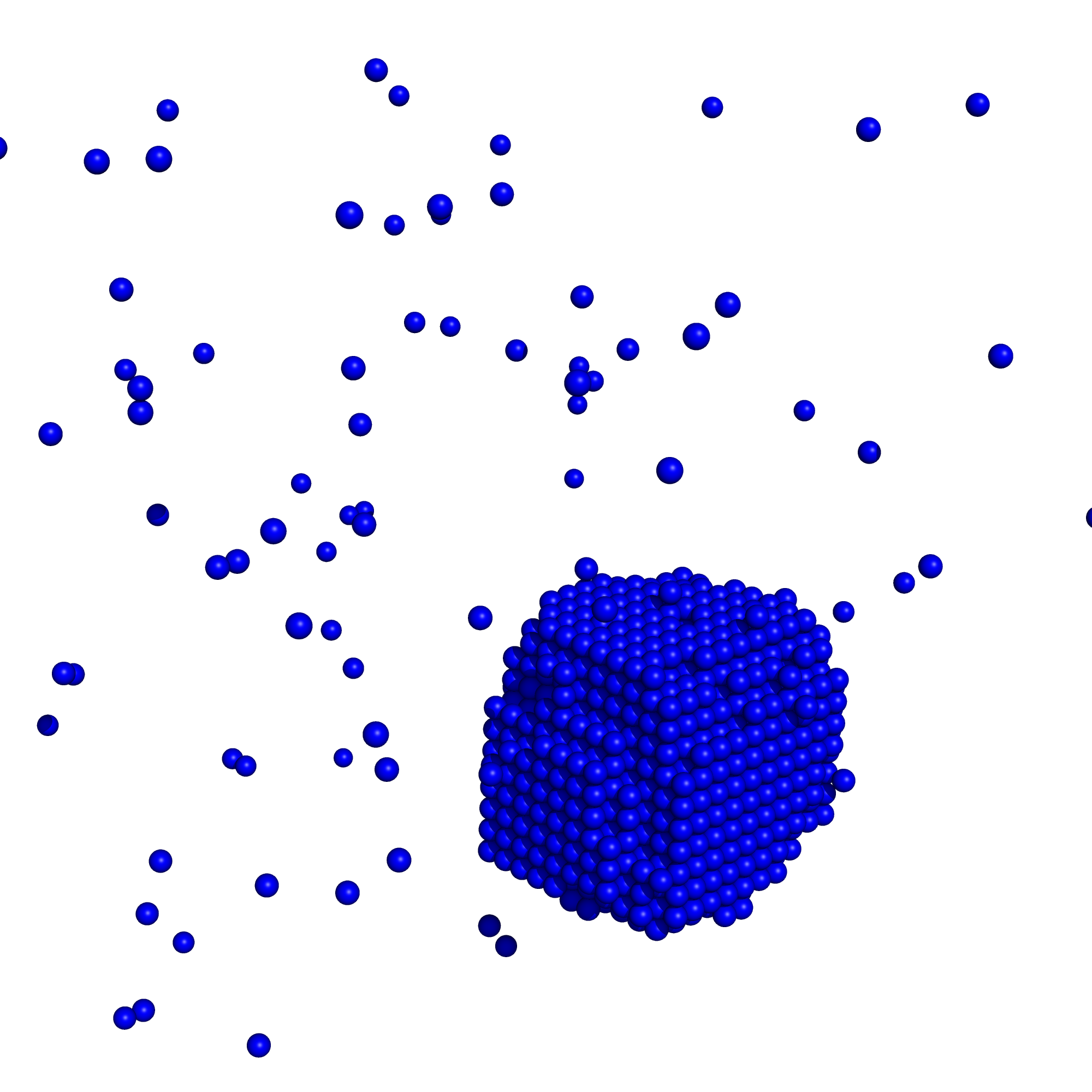
Figure 1: Example of (left) fluctuations of particle excess and (right) a single condensate in three dimensions.

This was translated into the language of the Ising spin model in [3, 7]. Here, we will concentrate on the formulation of a lattice gas, where each lattice site is either occupied by a particle or empty, i.e. $n_{i}\in\{0,1\}$. For a fixed number of particles this model is equivalent to the Ising model with spins $s_{i}\in\{-1,1\}$, at fixed total magnetization, when $s_{i}=2n_{i}-1$:

$$\mathcal{H}^{\rm gas}=-J\sum_{<i,j>}n_{i}n_{j}=\frac{1}{4}\mathcal{H}^{\rm Ising}+c(N)$$ (5)

Thus, for fixed coupling constants, a scaling of the temperature by $T^{\rm Ising}=T^{I}=4T$ and the addition of a system-size dependent constant transforms the energy scale of an Ising model into the corresponding one of a lattice gas. All other observables are then mapped accordingly by scaling the temperature.

The contributions to the free energy can as well be formulated in the language of a lattice gas. Consider a temperature-dependent vacuum or background density $\rho_{0}=N_{0}/V$, which may be identified with the spontaneous magnetization in the Ising model via

$$m_{0}=1-2\rho_{0}.$$ (6)

Adding particles to the system leads to a total particle excess $\delta N=N-N_{0}$. According to Biskup et al. this excess $\delta N$ may be decomposed into the particle excess inside the droplet $\delta N_{D}$ and the remaining particle excess in the fluctuating phase $\delta N_{F}$. For the infinite-size system and from the equivalence to the Ising model follows that the gas density is given by $\rho_{G}=\rho_{0}$ and the liquid density by $\rho_{L}=1-\rho_{0}$. Hence, in a droplet of size $V_{D}$ we expect an excess of particles $\delta N_{D}=(\rho_{L}-\rho_{G})V_{D}$. Introducing the fraction of excess particles inside a droplet $\lambda=\delta N_{D}/\delta N$, allows us to rewrite the decomposed particle excess as fractions $\delta N_{D}=\lambda\delta N$ and $\delta N_{F}=(1-\lambda)\delta N$. Altogether the total free energy $F=F_{\rm drop}+F_{\rm fluc}$ then reads

$$F=\left(\tau_{W}\left(\frac{\lambda\delta N}{1-2\rho_{0}}\right)^{\frac{d-1}{d}}+\frac{(1-\lambda)^{2}(\delta N)^{2}}{2\hat{\kappa}V}\right).$$ (7)

Rewriting the particle excess in terms of a volume

$$V_{L}=\frac{N-N_{0}}{1-2\rho_{0}}$$ (8)

and identifying $\lambda=V_{D}/V_{L}$ leads to

$$F = \left(\tau_{W}(\lambda V_{L})^{\frac{d-1}{d}}+\frac{(1-2\rho_{0})^{2}}{2\hat{\kappa}V}V_{L}^{2}(1-\lambda)^{2}\right)$$ (9)

$$= \tau_{W}V_{L}^{\frac{d-1}{d}}\left(\lambda^{\frac{d-1}{d}}+\Delta(1-\lambda)^{2}\right)$$

with the dimensionless parameter

$$\Delta = \frac{(1-2\rho_{0})^{2}}{2\hat{\kappa}\tau_{W}}\frac{V_{L}^{(d+1)/d}}{V}.$$ (10)

While $\hat{\kappa}$ has the same value as $\chi$ in the Ising model, $\tau_{W}$ has to be rescaled such that $\tau^{I}_{W}=4\tau_{W}$. At fixed temperature, the parameters $\rho_{0},\hat{\kappa},\tau_{W}$ are constant. Minimizing eq. (9) leads to the infinite-size solution for the equilibrium volume fraction $\lambda=\lambda(\Delta)$ (see [3, 4]). Biskup et al. showed that below a critical value $\Delta_{c}^{2D}\approx 0.9186$ or $\Delta_{c}^{3D}\approx 0.8399$ there are merely gas fluctuations, while above there exists one macroscopic droplet together with background fluctuations. At $\Delta_{c}$ the mass of the largest droplet jumps to a fraction $\lambda_{c}^{2D}=2/3$ or $\lambda_{c}^{3D}=1/2$ of the total particle excess. Droplets of intermediate size have negligible probability.

In order to compare to the analytic predictions, we have to measure the average size of the largest droplet at different densities but fixed temperature. Because of the increasing correlation times in large systems, we applied the multicanonical method, driving the system between the evaporated and condensed phase, and reweighted to the relevant temperatures afterwards. The energy ranges were obtained through short parallel tempering [16] runs in the beginning of each simulation.

4 Results

In order to assess the parallel algorithm, we performed two independent simulations of equivalent but different models, namely the Ising spin model and the lattice gas. While the lattice gas was simulated with the parallel multicanonical algorithm explained above, the Ising model was simulated with a Metropolis algorithm at fixed magnetization, also referred to as micromagnetic simulation. Both approaches needed independent simulation runs for each measurement point. We chose the inverse temperature in the Ising language to be $\beta^{I}=0.369$, which corresponds to a temperature $T=0.6995$ in the particle picture. Figure 2 shows very good agreement between the two completely independent and different methods.

A direct comparison of simulation times is rather difficult. For one, the multicanonical method provides additional information for various temperatures, and this comes at a price: A time-consuming weight iteration, which is not contributing to the production run. Whether or not the overhead of the initial weight iteration is justified, will depend on the desired size of the statistical error. Furthermore, the approaches will scale differently with system size, which we do not want to address at this point. For the plot in Fig. 2, the average simulation time per data point of both methods was about half an hour on common 2.5GHz cores, but the multicanonical simulation used 36 cores instead of one in the case of the micromagnetic simulation. However, with increasing system size the free-energy barrier between the evaporated and the condensed phase increases [17], and the necessary computation time for the single-core micromagnetic simulation exceeds the limits of practicability.

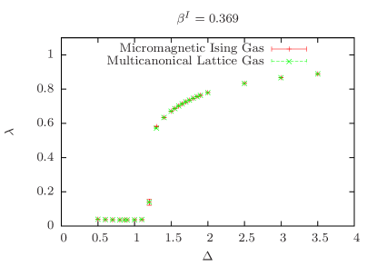
Figure 2: Comparison of simulation data from micromagnetic Metropolis simulations of the Ising model and parallel multicanonical simulations of the lattice gas in three dimension. Here, the volume is fixed at $L=30$ while the number of spins/particles are modified.

Next, we discuss the speedup of the parallel method with increasing degree of parallelization. As mentioned above, we intentionally did not pay attention to optimization of the simulation parameters. Rather we want to demonstrate the applicability of the parallelization by choosing appropriate parameters from single-process simulations. Hence, we fixed the total number of sweeps per iteration to $25600$ such that each process performed $25600/p$ sweeps. A single sweep consists of $L^{d}$ updates. The number of particles was chosen to be $N=1000$ and the energy range adapted accordingly. The simulation was defined to be converged if a total of 30 “tunneling events” were counted, meaning that the simulations had traveled at least 30 times from the maximal energy to the minimal energy or vice versa.

When we want to estimate the speedup, we need to consider statistical averages. This is due to the fact that the weight iteration relies on the sampled data such that the number of iterations until convergence cannot be predicted and may, moreover, vary depending on the initial seed of the random number generator. To this end, we performed 32 simulations for each degree of parallelization. The effect is best seen in the average number of iterations until convergence (Fig. 3 (a)). An increasing number of independent Markov chains improves each estimate of the distribution belonging to the current weights. This optimizes the estimation for the successive weights and reduces the total amount of necessary number of iterations. Of course, this is in general not true on all scales [9], for example when the number of sweeps per iteration becomes too small or if the optimal number of sweeps is more complex than the assumed $1/p$ behavior.

The speedup is defined in terms of the average time until convergence; it is given by the ratio of a single-core to a $p$-core simulation:

$$S_{p}=\frac{\bar{t}_{1}}{\bar{t}_{p}}.$$ (11)

For a fair comparison, both times were obtained with the same program. Because the communication between processes occurs only at the end of every iteration, the speedup should be ideal with a linear behavior of slope one, i.e., doubling the amount of processes should speed up the time by a factor 2. We can see in Fig. 3 (b) that this is indeed true for the case of three dimensions and even better for two dimensions. This may be explained by the reduced number of iterations, due to the independence of Markov chains.

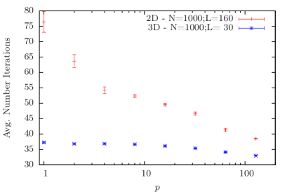
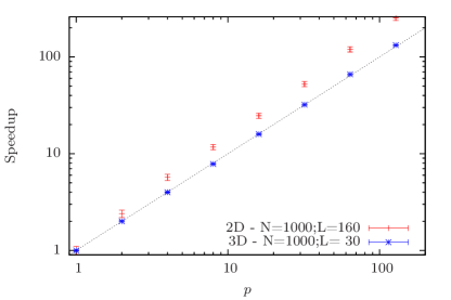
Figure 3: (a) Average number of iterations until convergence. (b) Average time speedup. The dotted line is a linear function of slope 1. Each average consists of 32 parallel multicanonical simulations.

Having demonstrated the correctness of our model and the efficiency of our method, we want to apply it to the problem of condensation in a lattice gas. Figure 4 shows the results for selected temperatures in two and tree dimensions with up to $24$ cores in each simulation. The temperature in two dimension was chosen to correspond to the equivalent Ising temperature $T^{I}=1.5$ used in Ref. [7], allowing us to use the same parameters. In three dimension we chose a temperature $T^{I}=2$ below the roughening transition $T^{I}_{R}\approx 2.4537$ [18], where low-temperature approximations hold. This allowed us to use a low-temperature series expansion for the interface tension: $\sigma=1.9072\dots$ [19]. Furthermore, below the roughening transition the condensate tends to form a cube, such that the surface free energy may be assumed as $\tau^{I}_{W}\approx 6\sigma$. This is the result for the Ising model and has to be rescaled by the same factor as the temperature, hence $\tau_{W}\approx 6\sigma/4$ (the same argument applies to the two-dimensional case). The remaining free parameters, $\rho_{0}=(1-m_{0})/2$ and $\hat{\kappa}=\chi$, were obtained by standard Metropolis simulations of the Ising model on very large lattices. An overview of the involved parameters is given in Table 1.

Table 1: Converted parameters for the lattice gas system in two [8] and three dimensions, where for the latter case $\rho_{0}=(1-m_{0})/2$ and $\hat{\kappa}=\chi$ are obtained from Metropolis simulations of the Ising model at various system sizes and $\tau_{W}\approx 6\sigma/4$ with $\sigma$ from a low-temperature expansion [19].

Parameter	2D	3D
$T$	0.375	0.500
$\rho_{0}$	0.00675	0.002739(1)
$\hat{\kappa}$	0.02708	0.00608(1)
$\tau_{W}$	1.06125	$\approx 2.861$

Opposite to Ref. [7], we always fixed the number of particles and varied the density by modifying the volume of the system. We can see in Fig. 4 that this choice leads to a similar behavior in two dimensions as in Ref. [7], where the predicted $\Delta_{c}$ separates the evaporated from the condensed phase quite well. Of course, we see finite-size effects as reported before, but the qualitative picture is satisfying. In three dimensions, on the other hand, we observe a strong deviation of small systems from the predicted critical value of the parameter $\Delta$. This becomes weaker but is still present for the largest systems investigated. Specifically, the system needs to go to larger $\Delta$ or, equivalently, particle density in order to condensate. With increasing system size, the critical value of $\Delta$ decreases, while the shape of the curves seems to converge to the predicted functional shape. This may be a finite-size effect that is more pronounced in three dimensions, which calls for more detailed studies in future work. In both cases, we do not have any free parameters left.

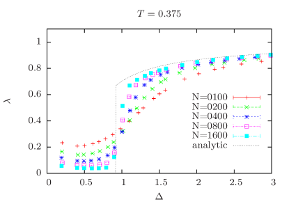
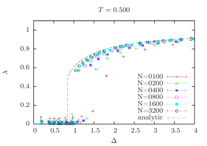
Figure 4: Condensation of a lattice gas in two (left) and three (right) dimensions. The temperature is chosen, such that the two-dimensional case corresponds to the Ising model at $T^{I}=1.5$ in Refs. [7, 8] and the three-dimensional case is below the roughening transition. The differently colored curves belong to fixed number of particles $N$, while the density is varied by changing $L$. Each data point corresponds to an independent simulation with up to $24$ cores.

5 Conclusion

We have demonstrated the applicability of an efficient but simple parallelization of the multicanonical method to the case of lattice gas condensation in two and three dimensions. In these cases, the speedup was shown to scale ideally (or even better) due to the fact that independent Markov chains improve the sampling of equilibrium distributions.

Applying this method to the problem of condensation, we could reproduce the results from [7] in two dimensions and present new results in three dimensions which indicate large finite-size effects. In the latter case, condensation systematically occurred at densities higher than predicted. While the deviation decreases with system size, the available data does not allow for quantitative predictions due to the low resolution at the critical density caused by varying the volume. This has still to be investigated in more detail.

References

References

- [1] Binder K and Kalos M H 1980 J. Stat. Phys. 22 363
- [2] Pleimling M and Selke W 2000 J. Phys. A 33
- [3] Biskup M, Chayes L and Kotecký R 2002 Europhys. Lett. 60 32
- [4] Biskup M, Chayes L and Kotecký R 2003 J. Stat. Phys. 116 175
- [5] Neuhaus T and Hager J S 2003 J. Stat. Phys. 113 47
- [6] Binder K 2003 Physica A 319 99
- [7] Nußbaumer A, Bittner E, Neuhaus T and Janke W 2006 Europhys. Lett. 75 716
- [8] Nußbaumer A, Bittner E and Janke W 2008 Phys. Rev. E 77 041109
- [9] Zierenberg J, Marenz M and Janke W 2013 Comput. Phys. Comm. 184 1155
- [10] Sugihara T, Higo J and Nakamura H 2009 J. Phys. Soc. Jpn. 78 074003
- [11] Slavin V V 2010 Low Temp. Phys. 36 243
- [12] Ghazisaeidi A, Vacondio F and Rusch L A 2010 J. Lightwave Technol. 28 79
- [13] Berg B A and Neuhaus T 1991 Phys. Lett. B 267 249
- [14] Berg B A and Neuhaus T 1992 Phys. Rev. Lett. 68 9
- [15] Janke W 1998 Physica A 254 164
- [16] Hukushima K and Nemoto K 1996 J. Phys. Soc. Japan 65 1604
- [17] Nußbaumer A, Bittner E and Janke W 2010 Prog. Theor. Phys. Suppl. 184 400
- [18] Hasenbusch M, Meyer S and Pütz M 1996 J. Stat. Phys. 85 383
- [19] Shaw L J and Fisher M E 1989 Phys. Rev. A 39 2189