DECAY PHASE COOLING AND INFERRED HEATING OF M- AND X-CLASS SOLAR FLARES

Abstract

In this paper, the cooling of 72 M- and X-class flares is examined using GOES/XRS and SDO/EVE. The observed cooling rates are quantified and the observed total cooling times are compared to the predictions of an analytical 0-D hydrodynamic model. It is found that the model does not fit the observations well, but does provide a well defined lower limit on a flare’s total cooling time. The discrepancy between observations and the model is then assumed to be primarily due to heating during the decay phase. The decay phase heating necessary to account for the discrepancy is quantified and found be $\sim$50% of the total thermally radiated energy as calculated with GOES. This decay phase heating is found to scale with the observed peak thermal energy. It is predicted that approximating the total thermal energy from the peak is minimally affected by the decay phase heating in small flares. However, in the most energetic flares the decay phase heating inferred from the model can be several times greater than the peak thermal energy.

1. Introduction

Solar flares are among the most powerful events in the solar system, releasing up to $10^{32}$ ergs in a few hours or even minutes. They are believed to be powered by magnetic reconnection, a process whereby energy stored in coronal magnetic fields is suddenly released. This causes a rapid heating and expansion of the flare plasma which is then believed to cool by conductive, radiative and enthalpy-based processes. However, the balance between cooling and heating in solar flares and the processes which determine this are still not fully understood. A greater insight into this interaction would allow us to better constrain the energy release mechanisms of solar flares.

To date there have been many studies aimed at modeling the heating and cooling of solar flares (e.g. Moore & Datlowe, 1975; Antiochos & Sturrock, 1978; Antiochos, 1980; Fisher et al., 1985; Doschek et al., 1983; Cargill, 1993; Klimchuk & Cargill, 2001; Reeves & Warren, 2002; Bradshaw & Cargill, 2005; Klimchuk, 2006; Warren, 2006; Warren & Winebarger, 2007; Sarkar & Walsh, 2008). These include full 3-D magnetohydrodynamic (MHD) models as well as 1-D MHD models. 1-D models assume that flare loop strands are magnetically isolated and therefore only solve the MHD equations along the axis of the magnetic field (e.g. Bradshaw & Cargill, 2005). This is less computationally draining than the full 3-D treatment and therefore allows a higher resolution, more useful for detailed comparison with observation. 0-D models have also been developed (e.g. Enthalpy-Based Thermal Evolution of Loops, EBTEL; Klimchuk et al., 2008) which treat field aligned average properties. Although these models sacrifice some completeness, they are much faster to run allowing an easier exploration of the dependence of results on different possible coronal property values. Although these models are valuable in increasing our understanding of flare heating and cooling they nonetheless suffer from drawbacks. These can include arbitrary inputs of unobservable parameters such as heating function and number of loop strands.

Previous studies focused on observations of flare cooling are also numerous. Culhane et al. (1970) compared simple collisional, radiative, and conductive cooling models to observations of four flares made with the fourth Orbiting Solar Observatory (OSO-4). They found that collisional cooling was unphysical while conduction and radiation were equally plausible. Although they could not determine which was dominant, they did find that that for radiative cooling to dominate, the flare density would have to be high ($\gtrsim$10¹¹ cm^-3). In contrast, conduction would require low densities ($\sim$10¹⁰ cm^-3) to dominate.

In contrast, Withbroe (1978) was able to compare the relative importance of cooling mechanisms. This study examined the differential emission measure (DEM) of a single flare using Skylab and hence determined that conductive and radiative losses were comparable. This suggests that both processes were equally important in the cooling of that flare. From discrepancies between observations and conductive and radiative cooling models, it was determined that $\sim$10³¹ ergs of additional heating must have been deposited after the flare peak.

More recently, Jiang et al. (2006) examined loop top sources in 6 flares using the Reuven Ramaty High Energy Solar Spectroscopic Imager (RHESSI; Lin et al., 2002). They found that the observed cooling rate was slightly higher than expected from radiative cooling, but significantly lower than that expected from conduction. To account for this, they calculated that more than 10³⁰ ergs of additional heating during the decay phase was necessary. This was greater than that seen during the impulsive phase. However they concluded that much of this discrepancy was more plausibly explained by suppressed conduction.

Raftery et al. (2009) also used RHESSI along with several other instruments to chart the thermal evolution of a single C1.0 flare. They performed a best fit to the observations using the EBTEL model and an assumed heating function to infer radiative and conductive cooling profiles. Conduction was found to dominate initially while radiation dominated in the latter phases.

A common aspect of many flare cooling studies such as those mentioned above is that they focus on single or small numbers of events. This means they cannot say if their findings are anomalous or characteristic of flares. As a result, it is still unclear just how well cooling models describe ensembles of flares. In this paper we aim to improve upon previous studies by observing the cooling profiles of 72 M- and X-class flares. This is done using observations from X-Ray Sensors onboard the Geostationary Operational Environmental Satellites (GOES/XRS; Hanser & Sellers, 1996) and the Extreme ultraviolet Variability Experiment onboard Solar Dynamics Observatory (SDO/EVE; Woods et al., 2012). The observed cooling times are then compared to predictions made by the model of Cargill et al. (1995), a simple, analytical 0-D model. Although this model is highly simplified, it was chosen as a first step because it is quick and easy to apply to many flares. In Section 2 of this paper we describe our observations. In Section 3 we discuss the assumptions, limitations and equations of the Cargill et al. (1995) model and describe how we observationally calculated the required inputs. In Section 4 we compare the observed cooling times to those predicted by the model and quantify the discrepancy. We then infer the decay phase heating required to account for this difference. Finally we outline our conclusions in Section 5.

2. Observations & Data Analysis

2.1. Instrumentation & Flare Sample

Observations for this study were taken from three instruments: the XRS onboard the GOES-14 and 15 satellites; the Multiple Extreme ultraviolet Grating Spectrograph A channel (MEGS A; Hock et al., 2012a) onboard SDO/EVE; and the X-Ray Telescope onboard Hinode (Hinode/XRT; Golub et al., 2007; Kano et al., 2008).

The GOES/XRS measures spatially integrated solar X-ray flux in two wavelength bands (long; 1–8 Å, and short; 0.5–4 Å) every two seconds. Temperature can be calculated from the ratio of these channels using the method of White et al. (2005). In this method, coronal abundances (Feldman et al., 1992), the ionization equilibria of Mazzotta et al. (1998), and a constant density of 10¹⁰ cm^-3 were assumed. Although this final assumption is probably not true, it was justified by White et al. (2005) who used CHIANTI to compute the spectrum of an isothermal plasma at 10 MK with densities of $10^{9}$, $10^{10}$, and $10^{11}$ cm^-3. No significant differences were found.

MEGS A onboard SDO/EVE measures spatially integrated solar irradiance from 6 to 37 nm with a spectral resolution of 0.1 nm. MEGS A is an 80^o grazing incidence off-Rowland circle spectrograph and has a time cadence of 10 s. Within its spectral range are a number of temperature and density sensitive Fe lines useful for examining the thermodynamics of hot flares.

Hinode/XRT is a grazing incidence X-ray telescope with a spatial resolution of 1 arcsec. It provides broadband images of the Sun in wavelengths of 0.2–20 nm. It has a maximum field of view of 34$\times$34 arcsecs but can also focus on several smaller regions of interest simultaneously. The time cadence depends on the observing program used but is typically on the order of seconds. Hinode/XRT has numerous filters which can help to reduce saturation during flares. These have quite wide temperature responses, but all peak around 8–13 MK. The temperature sensitivity, spatial resolution and time cadence of Hinode/XRT make it the most ideal instrument available for directly measuring loop lengths of hot ($>$5 MK) X-ray- and EUV-emitting flare plasma. It is better suited than the Atmospheric Imaging Assembly (AIA; Lemen et al., 2012) onboard SDO, which is often saturated by M- and X-class flares and which has greater sensitivity to cooler coronal plasma ($\sim$1 MK). However, of the 72 flares included in this study, only 22 were well observed by Hinode/XRT. Therefore, loop lengths were determined using the RTV-scaling law (Rosner et al., 1978) while Hinode/XRT was used to quantify the uncertainty of this law. See Section 3.2 for further details.

The 72 M- and X-class flares examined in this study were chosen via two criteria. Firstly, their decay phases had to be temporally isolated from other flares. This was determined from visual inspection of the GOES lightcurves. Secondly, the flares had to be observed to cool to at least 8 MK with either the GOES/XRS or SDO/EVE MEGS-A. A complete list of the flares and their properties are listed in Table 2 in the Appendix.

2.2. Observing Flare Cooling

Table 1Wavelengths and temperatures of bandpasses and emission lines used in measuring cooling rates

Instrument	Wavelength [nm]	Temperature [MK]
GOES/XRS	0.05–0.4 – Short 0.1–0.8 – Long	$>$4
Ion	Wavelength [nm]	Temperature [MK]
Fe XXIV	19.20	15.8
Fe XXII	11.71	12.6
Fe XIX	10.83	10.0
Fe XVIII	9.39	7.9
Fe XVI	33.54	6.3
Fe XV	28.41	2.5
Fe XIV	26.47	2.0

Figure 1.— Cooling track for the 2010-Nov-06 M5.5 flare which began at 15:28 UT. a) Background-subtracted GOES temperature profile. Peak is marked by the vertical line. b) – h) Lightcurves of sequentially cooler Fe lines ranging from 15.8 MK to 2 MK observed by SDO/EVE MEGS-A. The peak of each lightcurve is also marked by a vertical line. i) Combined cooling track obtained by plotting the time of the peak of each profile (including GOES temperature profile) with its associated peak temperature. The resultant cooling time is the duration of this cooling track.

The cooling of the flares in this study was charted by combining the peak of the GOES temperature profile with the peaks of lightcurves of various temperature sensitive Fe lines observed by SDO/EVE MEGS-A. The GOES temperature was calculated using the TEBBS method (Temperature and Emission measure-Based Background Subtraction; Ryan et al., 2012) which performs an automatic background subtraction and finds the temperature and emission measure using the method of White et al. (2005). The Fe lines used in this study along with their formation temperatures are listed in Table 1. These lines were chosen because in the conditions of a solar flare, they are dominant over neighbouring lines within the MEGS-A resolution and therefore minimally blended. Before extracting these lightcurves, a background subtraction was made to each observed flare spectrum. The background spectrum was found by averaging the spectra within a quiet period before the flare start time. This period was determined for each flare by visual inspection of the GOES lightcurves. This helped ensure that the behaviour of the lightcurves was minimally contaminated by emission from non-flaring plasma. The irradiance observed at the wavelength of each line in Table 1 was then summed with that within $\pm$0.05 nm, i.e. the spectral resolution of MEGS-A. This was done for each spectrum taken during the flare and hence flare lightcurves were formed. A cooling track was then generated by plotting the peak time of each lightcurve against its associated formation temperature. The cooling time was then given by the duration of this track.

Figure 2.— Histograms showing the non-linear (panel a) and linear (panel b) coefficients of the second order polynomial fits to the observed cooling profiles of the 72 M- and X-class flares in this study.

Figure 1 shows an example for an M5.5 flare which occurred on 2010 November 06 at 15:27 UT. Figure 1a shows the GOES temperature curve while Figures 1b–1h show the lightcurves of the Fe lines measured by SDO/EVE. The vertical lines in each panel mark the peak time of that lightcurve. The lightcurves peak in order of descending temperature. This is interpreted as being due to the plasma cooling. Figure 1i shows the resulting cooling track, with each datum point representing the peak time and temperature associated with the lightcurves above. From this it can be seen that this flare cooled from 17 MK to 2 MK over the course of 389 $\pm$ 10 seconds. The uncertainty comes from combining the time resolutions of the GOES/XRS and SDO/EVE in quadrature.

In order to parameterize the flare cooling, each flare’s cooling profile was fit with a second order polynomial of the form

$$T(t)=T_{0}+\theta t+\mu t^{2}\mbox{ MK}$$ (1)

where $t$ is time since the start of the cooling phase in seconds, $T_{0}$ is the temperature at the start of the cooling phase in megakelvin (i.e. GOES peak temperature), $\theta$ is the linear cooling coefficient [MK s^-1], and $\mu$ is the non-linear cooling coefficient [MK s^-2]. Figure 2a shows a histogram of the non-linear cooling coefficients, $\mu$. The distribution is very narrowly peaked around zero with a full width half max of $\lesssim$10^-4 MK s^-2 and a mean of -6$\times$10^-5 MK s^-2. This implies that the majority of the flare cooling profiles are very linear. This agrees qualitatively Raftery et al. (2009), whose observed cooling profile of a C1.0 flare was also quite linear. Figure 2b shows a histogram of the linear cooling coefficients, $\theta$. Since the non-linear cooling coefficients are so small, the linear cooling coefficients approximate the cooling rates. The histogram ranges from -1.5–0 MK s^-1 and has a mean of -0.035 MK s^-1. This implies that the SXR-emitting plasma of an average M- or X-class flare cools at a rate of $\sim$3.5$\times$10⁴ K s^-1. It should be noted that although the histogram in Figure 2b peaks at the bin centered on zero, all flares have non-zero linear cooling coefficients. These parameterizations are used again in Section 4.2.

3. Modelling

3.1. The Cargill Model

To model the cooling observations discussed in the previous section, we used the model of Cargill et al. (1995). This model is based on conductive and radiative cooling timescales derived from the energy transport equation which describes how a plasma’s thermal energy density changes with time. To derive these timescales, a number of assumptions are made. First, the plasma is isotropic, i.e. contains no shearing motions. Second, it is isothermal, i.e. obeys the ideal gas law, $p=Nk_{B}T$. Third, the plasma $\beta$ is low, implying all particle motions are along the axis of the magnetic field. Fourth, the plasma is ‘collisionless’. Fifth, the conductive heat flux obeys Spitzer conductivity, $\kappa_{0}T^{5/2}\nabla T$, where $\kappa_{0}=10^{-6}$. And sixth, the radiative loss function, $P_{rad}$, between 10⁶ and 10⁷ K is adequately modeled by $P_{rad}=\chi N^{\zeta}T^{\alpha}$ erg cm³ s^-1, where $\chi=1.2\times 10^{-19}$, $\zeta=2$ and $\alpha=-0.5$ (Rosner et al., 1978). By using these assumptions, the energy transport equation can be written as

$$\frac{1}{\gamma-1}\frac{\partial p}{\partial t}=-\frac{1}{\gamma-1}\frac{\partial}{\partial s}(pu_{s})-p\frac{\partial u_{s}}{\partial s}-\\ \left(\frac{\partial}{\partial s}\left[\kappa_{0}T^{5/2}\frac{\partial T}{\partial s}\right]-\chi N^{\zeta}T^{\alpha}\right)+h$$ (2)

where $p$ is pressure, $s$ is the spatial coordinate along the axis of the magnetic field, $u_{s}$ is the plasma velocity along the axis of the magnetic field, $T$ is temperature, $N$ is density, and $h$ is the heat energy added per unit volume, per unit time.

In order to derive the characteristic timescales of the cooling mechanisms, Cargill et al. (1995) assumed that there were no flows within the plasma ($u_{s}=0$) and that there was no heating ($h=0$). This implies that the only way the thermal energy density is altered is via conductive and radiative heat flux. Then the characteristic conductive cooling timescale can be derived by neglecting radiative processes in Equation 2, and vice versa for the characteristic radiative timescale. By further assuming that the plasma is monatomic (i.e. the adiabatic constant, $\gamma=5/3$) the conductive and radiative timescales are given by

$$\tau_{c}=4\times 10^{-10}\frac{NL^{2}}{T^{5/2}}$$ (3)

and

$$\tau_{r}=3.45\times 10^{3}\frac{T^{3/2}}{N}$$ (4)

respectively, where $L$ is loop half length.

From these timescales, a total cooling time can be calculated if it is assumed that the flare only cools by either conduction or radiation at any one time. If the conductive timescale is initially shorter than the radiative timescale, the flare is assumed to cool purely by conduction from its initial temperature, $T_{0}$, until time, $t_{*}$ and temperature, $T_{*}$, when the two timescales become equal. From then the flare is assumed to cool purely radiatively to the final temperature, $T_{L}$, which takes additional time, $t_{**}$. It should be noted here that $t_{*}$ and $t_{**}$ and different from $\tau_{c}$ and $\tau_{r}$. The former are the periods when the flare cools by conduction and radiation respectively. The latter are characteristic timescales of the cooling processes. With this in mind, the total cooling time of the flare is given by

$$t_{tot}=\tau_{c0}\left[\left(\frac{\tau_{r0}}{\tau_{c0}}\right)^{7/12}-1\right]+\\ \frac{2\tau_{r0}}{3}\left(\frac{\tau_{c0}}{\tau_{r0}}\right)^{5/12}\left[1-\left(\frac{\tau_{c0}}{\tau_{r0}}\right)^{1/6}\left(\frac{T_{L}}{T_{0}}\right)\right]$$ (5)

where subscript ‘0’ implies the value of that property at the start of the cooling phase. If conduction never dominates radiation, the flare is assumed to cool purely radiatively. This gives a total flare cooling time of

$$t_{tot}=\frac{2\tau_{r0}}{3}\left(1-\frac{T_{L}}{T_{0}}\right)$$ (6)

Equations 5 and 6 use the relations describing the temporal evolution of temperature due to conduction derived by Antiochos & Sturrock (1978) and due to radiation derived by Antiochos (1980).

The Cargill model is a very simple, easy-to-use analytical model. However, its simplicity gives rise to a number of limitations. It assumes that at any one time cooling occurs via either conduction or radiation, with an instant switch between the two when their cooling timescales are equal. This assumption may be an acceptable approximation when either the conductive or radiative timescales are much longer than the other. However, it is certainly not valid when the two timescales are similar. In addition, this model does not account for enthalpy-based cooling. This type of cooling is most significant towards the end of a flare when the temperature is low and no longer supports the plasma against gravity. Therefore these equations are not suitable for modeling plasma cooling below $\sim$1–2 MK.

Furthermore, the Cargill model treats the flare as a monolithic loop. Other 0-D models (e.g. Warren, 2006; Klimchuk et al., 2008) employ the idea that flaring loops are comprised of many smaller strands, each heated and cooled at different times. However, some recent studies (e.g. Aschwanden & Boerner, 2011; Peter et al., 2013) have examined coronal loop cross-sections at high resolution and found no discernible structure. This implies the such strands are below a resolution of 0.2 arcsec or that a monolithic treatment may be justified. If the flaring loops are indeed made of sub-strands they would have the same orientation. And since the plasma is frozen onto the magnetic field lines and diffusion across them is minimal, reducing the multiple strands to one spatial dimension along the axis of the magnetic field, as in the Cargill model, is somewhat justified via symmetry. One could argue something similar for multiple loops in a flaring arcade. However, this treatment implicitly assumes that all the loops/strands are being heated and cooled simultaneously which results in the average behavior of all the loops/strands being modeled. Despite this restriction, such an approach can still be useful in examining flare hydrodynamics, especially since the additional free parameters introduced by multi-strand modeling are very unwieldy when modeling a large number of flares.

Finally, the Cargill model does not account for heating which has been suggested can continue well into the decay phase (e.g. Withbroe, 1978; Jiang et al., 2006; Warren, 2006). Thus this assumption is not very well justified and would be expected to produce shorter predicted cooling times than those observed. Despite the above limitations, the Cargill model contains much of the physics believed to be responsible for flare cooling and quantifying how well it simulates observations is important to better understand flare evolution.

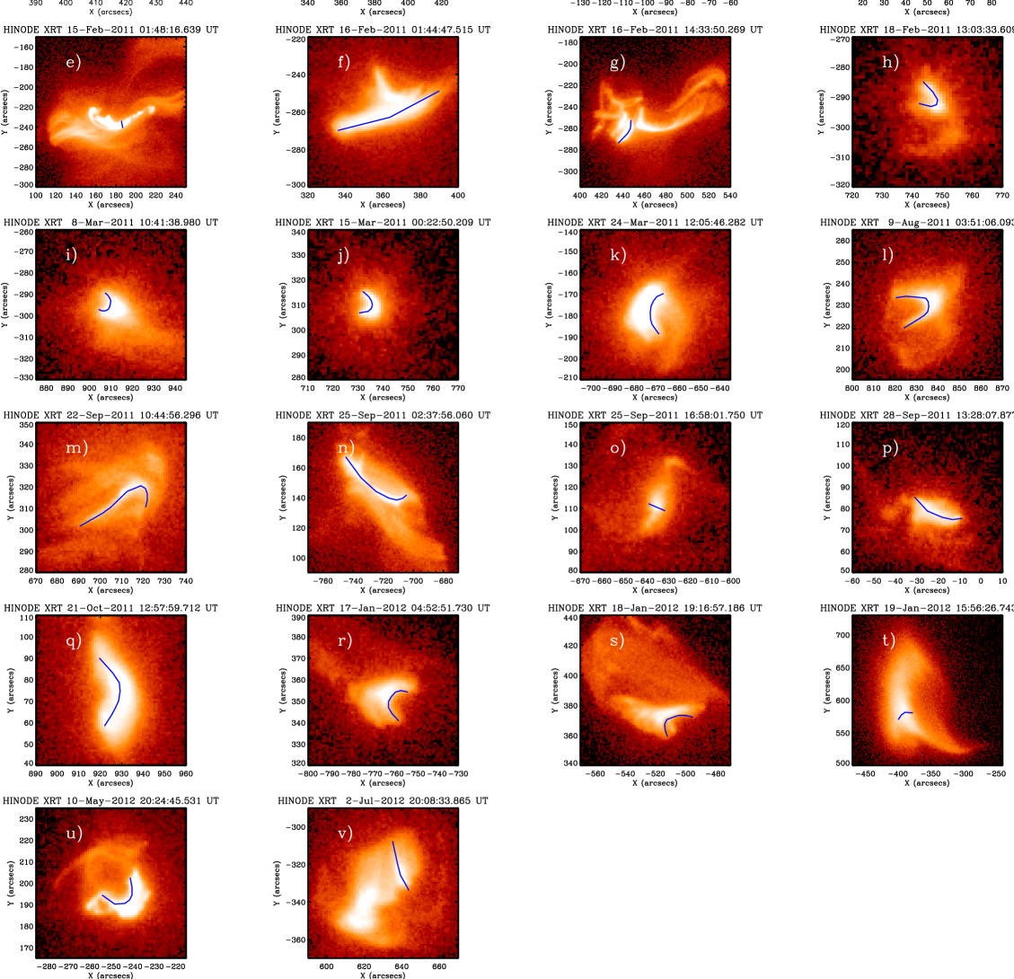
Figure 3.— Observed loop lengths measured with Hinode/XRT of 22 flares.

3.2. Observed Inputs to Cargill Model

The observed inputs required by the Cargill model are, initial temperature, initial density, and loop half length which is assumed to be constant.

The initial temperature, $T_{0}$, is that at the beginning of the observed cooling track i.e. the GOES temperature peak. As stated in Section 2.2 this was calculated using the TEBBS method (Ryan et al., 2012). This measurement has two sources of uncertainty: one due to the instrument (Garcia, 1994, Section 7) and one due to the background subtraction (Ryan et al., 2012, Section 3.2). The total uncertainty in the initial temperature was found by combining these two uncertainties in quadrature.

The initial density, $N_{0}$, was determined using the method of Milligan et al. (2012). This method uses CHIANTI (version 7; Landi et al., 2012) to determine the relationship between density and the ratios of three density dependent Fe XXI line pairs (12.121 nm/12.875 nm, (14.214 nm + 14.228 nm)/12.875 nm, and 14.573 nm/12.875 nm). In this study, only the first ratio was used as only these lines consistently exhibited increased emission due to the flares. This method is only valid for temperatures above 10 MK due to the formation temperatures of these lines. It is also not sensitive outside the range 10¹⁰–10¹⁴ cm^-3. However, the Cargill model only requires the initial density, i.e. the density at the time of the peak GOES temperature. Since all the flares in this study peak above 10 MK and were found to have densities within this range, the method of Milligan et al. (2012) is suitable.

The uncertainty in the density measurement was taken from the uncertainty in the line intensity ratio as measured by EVE. The ratio itself has two main sources of uncertainty. First, the instrumental uncertainty of the irradiance of the two lines. Second is the uncertainty due to the noise in the ratio time profile. The latter was evaluated as the standard deviation during the time period when the flare was hotter than 12 MK as determined with the GOES/XRS. This threshold was chosen as it ensured that the flare temperature (accounting for uncertainty) was in the valid range of the Milligan et al. (2012) method. The total uncertainty in the ratio was determined from the standard propagation of errors of the two uncertainty sources. This uncertainty was then transformed to density by propagating the ratio’s upper and lower limits as per Milligan et al. (2012). It should be noted that there are additional uncertainties associated modelled relationship between FeXXI line intensities and density. However, these are expected to be much smaller than the uncertainty sources discussed above. For more information on the modelling of the FeXXI lines in CHIANTI see Section 4.7.1 of Dere et al. (1997), and references therein.

Figure 4.— Comparison of RTV-predicted flare loop half lengths with those measured with Hinode/XRT. A loose correlation can be seen around the 1:1 line (over-plotted).

As stated in Section 2.1, loop half length, $L$, was determined using the RTV scaling law (Rosner et al., 1978)

$$L=(1.4\times 10^{3})^{-3}\left(\frac{T_{max}^{3}}{p}\right)$$ (7)

where $p$ is pressure and $T_{max}$ is the maximum temperature in the loop. By assuming that the plasma is isothermal and obeys the ideal gas law, this can be rewritten in terms of temperature, $T$, and density, $N$, which can be calculated using GOES/XRS and SDO/EVE respectively.

$$L=\frac{1}{k_{B}(1.4\times 10^{3})^{3}}\frac{T^{2}}{N}$$ (8)

Ideally, these loop half lengths would be directly measured using Hinode/XRT. However, only 22 of the events in this study were well-observed by this instrument and so it was necessary to utilize the RTV-scaling.

In order to quantify the uncertainties of the RTV-predicted values, the loop lengths of these 22 events were measured with Hinode/XRT (Figure 3). These are plain-of-sky measurements performed ‘by eye’. A more rigorous analysis attempting to account for projection affects is expected to alter the measured loop lengths only up to a factor of $\sim$2 which is sufficient for our purposes. The different XRT filters used for each event can be found in Table 2 in the Appendix. These filters all peak between 8–13 MK. Their response functions show contributions from plasma at temperatures below 1 MK of at least 2 orders of magnitude lower than the peak. This suggests that the images are not significantly contaminated by emission from lower temperature plasma which might otherwise affect the measured loop lengths. The one exception is the Al-mesh filter. But this was only used for one event and was not found to be an outlier. Where possible, SDO/AIA was used to help determine the axis of the magnetic field, along which the loop length should be measured. For instance, a combination of AIA and XRT movies revealed that the long axis of the flares in the panels e), o), t) of Figure 3 were flare arcades and the loop lengths themselves were actually along the shorter axis. Despite its usefulness in these instances, AIA’s sensitivity to cooler plasma and greater tendency to saturate made it less well suited to making the actual measurements than XRT. The loop half lengths implied by the XRT measurements were compared to the RTV-predicted values (Figure 4) and a loose correlation around the 1:1 line was found.

Figure 5.— Comparison of Cargill-predicted cooling times with observed cooling times. The 1:1 line is overplotted for clarity.

The CVRMSD (coefficient of variation of the root-mean-square deviation) of the distribution in Figure 4 was used to quantify the uncertainty of the RTV-predicted loop half lengths. This was found to be 1.8, implying that the loop half length and uncertainty is given by $L=L_{RTV}\pm 1.8\cdot L_{RTV}$. This compares favourably with Aschwanden & Shimizu (2013) who compared RTV-predicted loop lengths with the length-scales of less intense flares using SDO/AIA and found an uncertainty of $\pm 1.6\cdot L_{RTV}$.

Having measured the initial temperature, initial density and loop half length, the Cargill-predicted cooling times were found from Equation 5 if $\tau_{c0}<\tau_{r0}$ and Equation 6 if $\tau_{c0}>\tau_{r0}$. The uncertainties on these cooling times were calculated by first rewritting Equations 5 and 6 in terms the observed input properties (temperature, density and loop half length) and then propagating their uncertainties by the standard error propagation rules. Having done this, we then compared the model-predicted cooling times with the observations discussed in Section 2.2.

4. Results & Discussion

4.1. Comparing Observed and Modeled Cooling Times

Figure 5 shows the comparison of Cargill-predicted and observed cooling times for 72 M- and X-class flares. The 1:1 line is over-plotted for clarity. It can clearly be seen that Cargill is consistent with observations at the shortest cooling times, but is not a good overall fit to the distribution. Upon closer inspection it was found that only 14 events (20%) had observed cooling times which agreed with Cargill within experimental error. Meanwhile 58 (80%) disagreed. Of those, only 1 was over-estimated by Cargill. The remaining 57 were underestimated. Thus these results statistically prove that the Cargill model provides a lower limit to the time needed for a flare to cool. In addition, it was found in 52 flares (72%) that radiation dominated conduction for the entirety of the cooling phase. Conduction initially dominated radiation in only 20 flares (28%). This suggests that flares for which radiation is the dominant cooling mechanism (such as those examined by McTiernan et al., 1993; López Fuentes et al., 2007) are far more common than those in which conduction initially dominates (e.g.  Moore & Datlowe, 1975; Jiang et al., 2006; Raftery et al., 2009). Furthermore, Culhane et al. (1970) concluded from examining a simple radiative cooling model that flare plasma cooling by radiation in a timescale of $\sim$500 s would exhibit high densities (10¹¹–10¹² cm^-3). The average observed cooling time of the events in Figure 5 is 653 s and their average density is 1.4$\times$10¹² cm^-3, which is very close to the conclusions of Culhane et al. (1970). This strengthens the claim that radiation is typically dominant over conduction throughout a flare’s decay phase.

To further quantify the discrepancy between predicted and observed cooling times (henceforth referred to as the ‘excess cooling time’), the root-mean-square deviation (RMSD) of the distribution was calculated. This was found to be 961 s. Normalizing this to the mean of the observed cooling times (653 s) gives the coefficient of variation of the root-mean-square deviation (CVRMSD). This quantifies the spread of the ‘excess cooling times’ relative to the mean of the observed cooling times. The CVRMSD was found to be 1.47 indicating a large spread as is visually suggested in Figure 5.

If the Cargill model is adequately describing the cooling mechanisms of solar flares, the ‘excess cooling time’ suggests that there is additional heating occurring throughout the decay phase. Similar assumptions have been made in previous studies (e.g. Withbroe, 1978; Jiang et al., 2006; Hock et al., 2012b). In the following section we explore just how much additional heating energy is required to account for the ‘excess cooling times’ and examine the distributions of these energies.

4.2. Inferring Heating During Decay Phase

For radiatively dominated flares, the decay phase heating required to account for the ‘excess cooling time’ can be determined from the following modified version of the energy transport equation

$$3k_{B}N_{0}\frac{\partial T}{\partial t}=-\chi N_{0}^{\zeta}T^{\alpha}+h$$ (9)

where $k_{B}$ is Boltzmann’s constant, $N_{0}$ is the density (assumed to be constant and equal to the initial density to remain consistent with the Cargill model), $T$ is temperature, $t$ is time, $\chi$, $\zeta$ and $\alpha$ have the same values as above (1.2 $\times$ 10^-19, 2, and -0.5, respectively), and $h$ is the heating rate per unit volume. This equation is stating that the rate of change of thermal energy density (LHS), is determined by the radiative energy losses (1st term, RHS) and heating (2nd term, RHS). The total decay phase heating energy, $H$, can then be evaluated by integrating over time and multiplying by flare volume, $V$, assumed to be constant.

$$H=V\times\\ \int_{0}^{t_{tot}}\left[3k_{B}N_{0}\frac{\partial T(t)}{\partial t}+1.2\times 10^{-19}N_{0}^{2}T(t)^{-1/2}\right]dt$$ (10)

This analysis was performed on 38 flares within our sample (marked in Table 2 in the Appendix by their non-zero values in the ‘Decay Phase Heating’ column). These flares were chosen because the Cargill model implied that radiation was the dominant cooling mechanism throughout their decay phases, making Equations 9 and 10 valid. These flares were also seen to cool down to at least 6 MK so the majority of their cooling could be analyzed. The rate of change of temperature, $dT/dt$, in Equation 10 was found by differentiating the second order polynomial fits to the cooling profiles discussed in Section 2.2. The flare volume was calculated from the density and peak emission measure using the equation,

$$V=\frac{EM}{N^{2}}$$ (11)

The emission measure was calculated from ratio of the GOES long channel flux and temperature using the same assumptions and methods as described in Section 2.1 (White et al., 2005; Ryan et al., 2012, TEBBS). The total decay phase heating required to account for the ‘excess cooling time’ was then calculated from Equation 10.

Figure 6.— Heating during the decay phase as a function of the difference between the observed and Cargill-predicted cooling times for 38 M- and X-class flares. The line over-plotted is the best fit to the data (see Equation 12).

Figure 7.— Histograms showing the required total heating during the decay phase of 38 M- and X-class flares to account for the difference between the Cargill-predicted observed cooling times (‘excess cooling time’). a) Log₁₀ of total decay phase heating. b) Total decay phase heating normalized by the total energy radiated by the flare as measured by GOES. c) Total decay phase heating divided by the thermal energy at the beginning of the cooling phase.

Figure 6 shows resultant energies as a function of the ‘excess cooling time’. The Pearson correlation coefficient of the distribution was calculated in log-log space and found to be 0.77, implying a statistically significant correlation. The following power-law was fit to the data,

$$H=10^{26.73}(\Delta t)^{1.06\pm 0.24}$$ (12)

where $H$ is the total heating energy during the decay phase, and $\Delta t$ is the ‘excess cooling time’. The uncertainty on the exponent represents one standard deviation. This power-law quantifies, in very simple terms, the affect of heating during the decay phase on a flare’s cooling time.

Figure 7a shows a histogram of these energies which range from 2$\times$10²⁸ – 5$\times$10³⁰ ergs. The findings of Withbroe (1978) and Jiang et al. (2006) fit into the upper limit of this range. They inferred total decay phase heating of 10³¹ ergs for the 1973 September 7 flare and $>10^{30}$ ergs in the 2002 September 20 flare, respectively. Although the energies in Figure 7a are plausible, further testing of the Cargill model is necessary to categorically prove whether they are correct. Nonetheless, from these heating calculations, it is possible to work out some implications of these energies in fact being correct. This provides extra ways of testing the Cargill model’s accuracy.

Firstly, the distribution in Figure 7a was fit with an an exponential using the method of maximum-likelihood, resulting in,

$$f(H)\propto e^{-\gamma\cdot H}$$ (13)

where $f(H)$ is the number of events as a function of total decay phase heating energy, $H$, and $\gamma~{}=~{}1.7~{}(\pm 0.3)~{}\times~{}10^{-30}$. Again, the uncertainty represents one standard deviation. An exponential fit was chosen because the Kolmogorov-Smirnov test (Wall & Jenkins, 2003, Chapter 5: Hypothesis Testing) implied it was best suited to the data. However energy frequency distributions of solar flares are often found to be power-laws (e.g. Aschwanden, 2011) which may be due to self-organized criticality. In this case, we cannot rule out the possibility that selection effects may have biased this distribution and including more events might reveal it to be more power-law-like. With this in mind, a power-law was also fit to this distribution via the method of maximum-likelihood and found to be

$$f(H)\propto H^{-0.6\pm 0.1}$$ (14)

Next, the values in Figure 7a were compared to the total thermally radiated energy (Figure 7b). CHIANTI was used to determine the spectra corresponding to the temperature and emission measure as calculated from GOES. The total radiated energy was then found by integrating over all wavelengths and over flare duration. The distribution in Figure 7b ranges from 0.2–0.9 and peaks at 0.5. As previously stated, the Cargill model implies that radiation is the dominant loss mechanism for these flares. If this is true, Figure 7b suggests that the total heating during the decay phase typically makes up half of the flare’s total thermal energy budget.

The significance of the total decay phase heating is further highlighted in Figure 7c where it has been normalized by the thermal energy at the flare peak, calculated from the following equation.

$$E_{peak}=3Nk_{B}T$$ (15)

The distribution has a negative slope and ranges from $<$1 to $>$7. This implies that the total decay phase heating energy inferred from the ‘excess cooling time’ can be several times greater than the thermal energy at the peak. This agrees with Jiang et al. (2006) who found that the inferred decay phase heating in the 2002 September 20 event was greater than the energy deposited during the impulsive phase. Such a result would be significant as previous studies (e.g.  Emslie et al., 2012) have used peak thermal energy as an estimate for the total thermal energy of a flare. To quantify the relationship between decay phase heating, $H$, and peak thermal energy, $E_{peak}$, a power-law was fit to the data and found to be

$$H=10^{-2.7\pm 0.4}E_{peak}^{1.1\pm 0.1}$$ (16)

This implies that the total decay phase heating as a fraction of the peak thermal energy is greater for greater values of the peak thermal energy. In the range explored here, the average total decay phase heating is $\sim$2.5 times the peak thermal energy. However, this is expected to be less for less energetic flares. Thus if the ‘excess cooling times’ inferred from the Cargill model are to be believed, estimating a flare’s total thermal energy from its peak is valid for small flares, but not for the most energetic events.

The predictions and comparisons made here all assume that the total decay phase heating inferred from the Cargill model is reasonable. These predictions give further ways of testing the validity of the Cargill model via observations or more advanced modeling of decay phase heating.

5. Conclusions

In this paper, the cooling phases of 72 M- and X-class solar flares were examined with GOES/XRS and SDO/EVE. The cooling profiles as a function of time were parameterized and typically found to be very linear. The average cooling rate was found to be $\sim$3.5$\times$10⁴ K s^-1. These observations were compared to the predictions of the Cargill et al. (1995) model. Loop half lengths needed by this model were calculated via the RTV scaling law (Rosner et al., 1978). The uncertainty on this law was quantified by comparing the predicted lengths of 22 flares within the sample with observations made by Hinode/XRT. The loop half lengths predicted by RTV scaling law were typically within a factor of 3 of those seen in Hinode/XRT.

It was found that the Cargill model provides a well defined lower limit on flare cooling times, and the deviation from the model was quantified. The root-mean-square deviation between the observations and the model was found to be 961 s and which was 1.47 of the mean observed cooling time. Furthermore, the Cargill model finds that radiation is the dominant loss mechanism throughout the cooling phase for 80% of flares. For the remaining 20%, Cargill finds that conduction dominates initially, before being superseded by radiation.

Next, the ‘excess cooling time’ was assumed to be due to additional heating. The total decay phase heating required to account for the ‘excess cooling time’ was inferred for 38 flares within the sample. The energies were found to be physically plausible, ranging from 2$\times$10²⁸ – 5$\times$10³⁰ ergs. The frequency distribution could be described by either an exponential with an exponent of $-1.7(\pm 0.3)\times 10^{-30}$ or a power-law with an exponent of $-0.6\pm 0.1$. These total decay phase heating energies were found to be highly correlated with the ‘excess cooling time’ and was fit with a power-law with an exponent of 1.06$\pm$0.24 and a scaling factor of $10^{26.73}$. It was also found that the total decay phase heating predicted from the Cargill model typically makes up about half of the thermally radiated energy budget of the hot flare plasma. Finally, it was determined that if the decay phase heating inferred from the Cargill model is to be believed, then peak thermal energy is an acceptable estimate for the total thermal energy of small flares. However, this method would underestimate the thermal energy budget for the most energetic events.

In order to confirm of refute the findings inferred using the Cargill model, comparisons with direct observations of the decay phase heating must be made for an ensemble of flares. This would further highlight the strengths and weaknesses of the Cargill model. In addition, including more temperature sensitive lines in a similar analysis to this one or performing fits of the full EVE observed spectrum would give more comprehensive observations of the temperature and density evolution of the flare plasma. Studies comparing similar observations with results of more advanced hydrodynamic simulations would also help us better understand the thermodynamic evolution and energetics of flare decay phases.

We would like to thank the anonymous referee for providing constructive feedback on this manuscript. DFR would like to thank Arthur J. White, Trevor A. Bowen, Dr. Jim Klimchuk, Dr. Joel C. Allred and Dr. C. Alex Young for their helpful discussions. He would also like to thank the Fulbright Association for funding the research. PCC and DFR would like to acknowledge funding from the Living With a Star Targeted Research and Technology Program. ROM is grateful to the Leverhulme Trust for financial support from grant F/00203/X, and to NASA for LWS/TR&T grant NNX11AQ53G.

Table 2Events used in this study with observed and model-predicted cooling times and other thermodynamic properties

Date	GOES	GOES	Observed	Cargill	T Peak	T Peak	T Min	T Min	Density	Loop Half	XRT Half	XRT Filter	Decay Ph.
	Start Time	Class	Cooling [s]	Cooling [s]	[MK]	Time [s]	[MK]	Time [s]	[1012 cm-3]	Length [cm]	Length [cm]		Energy [ergs]
2010 May 05	17:13:00	M1.3	212	241	21.0	17:17:59	2.5	17:21:31	0.9	1.0	0.5	Al_thick	(…)
2010 Jun 12	00:30:00	M2.0	295	112	20.6	00:56:13	1.6	01:01:09	1.8	0.7	(…)	(…)	1.2
2010 Jun 13	05:30:00	M1.0	267	55	15.4	05:37:12	7.9	05:41:39	1.2	0.7	(…)	(…)	(…)
2010 Oct 16	19:07:00	M3.2	115	122	17.3	19:11:44	2.5	19:13:40	1.2	1.0	1.2	Al_mesh	(…)
2010 Nov 06	15:27:00	M5.5	389	257	17.4	15:35:06	2.0	15:41:35	0.6	1.8	(…)	(…)	3.4
2011 Feb 09	01:23:00	M1.9	112	154	16.9	01:30:18	2.5	01:32:11	0.9	0.8	(…)	(…)	(…)
2011 Feb 13	17:28:00	M6.6	422	113	20.4	17:34:30	2.5	17:41:32	1.6	1.0	1.7	Ti_poly	4.2
2011 Feb 14	17:20:00	M2.3	128	50	17.9	17:24:44	2.5	17:26:52	3.0	0.5	0.4	Be_thick	0.5
2011 Feb 15	01:44:00	X2.3	501	213	24.5	01:53:20	2.5	02:01:42	1.2	1.7	0.3	Be_thin	(…)
2011 Feb 16	01:32:00	M1.0	540	187	17.5	01:37:52	7.9	01:46:53	0.6	1.3	2.1	Ti_poly	(…)
2011 Feb 16	14:19:00	M1.7	118	66	15.9	14:24:44	6.3	14:26:43	1.3	0.7	0.9	Be_thin	0.3
2011 Feb 18	12:59:00	M1.5	215	112	20.1	13:02:28	2.5	13:06:03	1.6	2.2	0.6	Be_thick	0.5
2011 Mar 07	07:49:00	M1.6	196	88	21.4	07:52:21	7.9	07:55:38	1.5	0.3	(…)	(…)	(…)
2011 Mar 07	09:14:00	M1.8	157	77	17.6	09:19:01	7.9	09:21:38	1.6	0.4	(…)	(…)	(…)
2011 Mar 08	03:37:00	M1.5	2025	209	13.0	03:46:13	2.5	04:19:58	0.4	1.7	(…)	(…)	8.2
2011 Mar 08	10:35:00	M5.4	386	85	20.2	10:41:02	2.5	10:47:28	2.1	0.7	0.5	Be_thick	2.9
2011 Mar 09	23:13:00	X1.5	542	181	23.8	23:21:36	2.5	23:30:38	1.3	1.6	(…)	(…)	13.4
2011 Mar 15	00:19:00	M1.1	140	82	19.6	00:22:20	2.5	00:24:40	2.1	0.8	0.5	Be_thick	(…)
2011 Mar 24	12:01:00	M1.0	341	107	16.7	12:06:01	2.5	12:11:43	1.2	0.7	0.8	Al_med	0.6
2011 Jul 27	15:48:00	M1.1	959	48	14.0	15:59:24	7.9	16:15:23	1.1	1.0	(…)	(…)	(…)
2011 Aug 03	04:29:00	M1.7	136	60	19.7	04:31:39	6.3	04:33:55	2.3	0.9	(…)	(…)	0.3
2011 Aug 04	03:41:00	M9.3	451	194	18.0	03:54:14	2.0	04:01:45	0.8	1.3	(…)	(…)	7.2
2011 Aug 09	03:19:00	M2.5	1430	310	17.7	03:49:06	2.5	04:12:56	0.6	1.1	1.2	Al_thick	(…)
2011 Aug 09	07:48:00	X7.3	233	225	32.5	08:03:23	1.6	08:07:16	1.8	1.9	(…)	(…)	(…)
2011 Sep 07	22:32:00	X1.8	281	145	21.8	22:37:42	2.5	22:42:24	1.4	1.0	(…)	(…)	6.4
2011 Sep 22	10:29:00	X1.4	2934	378	20.2	10:44:13	7.9	11:33:08	0.4	2.7	1.7	Al_thick	(…)
2011 Sep 24	17:19:00	M3.1	498	10	19.5	17:22:10	7.9	17:30:28	10.9	0.3	(…)	(…)	(…)
2011 Sep 25	02:27:00	M4.6	228	125	20.1	02:31:54	2.5	02:35:43	1.4	1.0	1.9	Al_med + Al	0.9
2011 Sep 25	04:31:00	M7.4	1152	209	18.2	04:39:56	2.5	04:59:09	0.7	2.0	(…)	(…)	13.5
2011 Sep 25	15:26:00	M3.8	325	108	15.7	15:32:44	2.5	15:38:09	1.1	0.7	0.3	Be_thick	2.3
2011 Sep 25	16:51:00	M2.2	202	272	18.5	16:55:36	2.5	16:58:59	0.6	1.5	(…)	(…)	(…)
2011 Sep 28	13:24:00	M1.3	240	76	17.9	13:27:29	2.5	13:31:30	2.0	0.6	0.9	Al_med	0.6
2011 Oct 02	00:37:00	M3.9	681	215	21.0	00:45:59	2.0	00:57:20	0.9	2.0	(…)	(…)	5.2
2011 Oct 20	03:10:00	M1.6	1360	1825	32.4	03:15:25	7.9	03:38:06	0.2	10.9	(…)	(…)	(…)

Date	GOES	GOES	Observed	Cargill	T Peak	T Peak	T Min	T Min	Density	Loop Half	XRT Half	XRT Filter	Decay Ph.
	Start Time	Class	Cooling [s]	Cooling [s]	[MK]	Time [s]	[MK]	Time [s]	[1012 cm-3]	Length [cm]	Length [cm]		Energy [ergs]
2011 Oct 21	12:53:00	M1.3	426	260	16.3	12:57:27	2.5	13:04:33	0.6	0.9	1.3	Al_med	(…)
2011 Oct 31	14:55:00	M1.1	2033	92	29.0	15:00:45	7.9	15:34:39	2.8	1.2	(…)	(…)	(…)
2011 Dec 25	18:11:00	M4.1	197	130	18.9	18:15:15	2.5	18:18:33	1.3	1.2	(…)	(…)	1.2
2011 Dec 26	02:13:00	M1.5	787	151	17.2	02:22:06	2.5	02:35:13	0.9	1.3	(…)	(…)	2.2
2011 Dec 29	21:43:00	M2.0	393	124	18.2	21:48:00	7.9	21:54:34	0.8	2.1	(…)	(…)	(…)
2012 Jan 17	04:41:00	M1.0	942	88	15.1	04:46:06	6.3	05:01:49	0.9	1.2	0.8	Al_med	1.8
2012 Jan 18	19:04:00	M1.7	461	122	15.9	19:09:08	2.5	19:16:50	1.0	1.2	1.1	Al_med	1.5
2012 Jan 19	13:44:00	M3.2	5318	50	14.3	15:14:51	7.9	16:43:30	1.1	0.9	1.0	Be_thick	(…)
2012 Jan 23	03:38:00	M8.7	1427	171	18.6	03:49:43	1.6	04:13:31	1.0	1.4	(…)	(…)	23.4
2012 Feb 06	19:31:00	M1.0	2783	340	12.9	19:42:31	2.0	20:28:55	0.2	0.7	(…)	(…)	(…)
2012 Mar 05	02:30:00	X1.1	2499	142	19.1	03:52:33	6.3	04:34:12	0.9	1.4	(…)	(…)	46.9
2012 Mar 06	12:23:00	M2.2	1369	128	18.3	12:36:54	7.9	12:59:43	0.8	1.4	(…)	(…)	(…)
2012 Mar 06	21:04:00	M1.4	365	126	18.0	21:06:18	7.9	21:12:23	1.0	0.7	(…)	(…)	(…)
2012 Mar 06	22:49:00	M1.0	321	62	19.0	22:52:31	2.5	22:57:53	2.6	0.5	(…)	(…)	0.5
2012 Mar 14	15:08:00	M2.8	397	113	16.0	15:17:38	2.0	15:24:15	1.1	0.9	(…)	(…)	1.9
2012 Mar 17	20:32:00	M1.4	264	184	19.0	20:37:41	2.0	20:42:06	1.0	1.1	(…)	(…)	(…)
2012 Mar 23	19:34:00	M1.0	172	138	18.5	19:39:35	7.9	19:42:28	1.0	0.7	(…)	(…)	(…)
2012 Apr 27	08:15:00	M1.1	616	103	14.8	08:22:32	2.5	08:32:48	1.1	1.3	(…)	(…)	1.4
2012 May 07	14:03:00	M1.9	1410	312	14.6	14:18:50	2.5	14:42:20	0.3	2.0	(…)	(…)	5.3
2012 May 08	13:02:00	M1.4	150	57	18.4	13:06:30	6.3	13:09:00	2.4	0.2	(…)	(…)	(…)
2012 May 10	04:11:00	M5.9	258	43	18.5	04:16:52	6.3	04:21:11	2.8	0.4	(…)	(…)	2.6
2012 May 10	20:20:00	M1.8	328	45	16.3	20:23:23	2.5	20:28:51	2.8	0.3	0.9	Ti_poly	1.1
2012 May 17	01:25:00	M5.1	1256	139	15.8	01:38:06	6.3	01:59:03	0.6	1.7	(…)	(…)	12.4
2012 Jun 03	17:48:00	M3.4	231	97	14.9	17:54:26	2.0	17:58:17	1.2	0.7	(…)	(…)	1.9
2012 Jun 09	16:45:00	M1.9	200	193	18.5	16:50:17	2.5	16:53:38	1.0	0.8	(…)	(…)	(…)
2012 Jun 10	06:39:00	M1.3	317	107	17.5	06:43:21	6.3	06:48:38	1.0	1.1	(…)	(…)	0.7
2012 Jun 30	12:48:00	M1.1	130	64	17.3	12:51:33	6.3	12:53:43	1.6	1.0	(…)	(…)	0.2
2012 Jun 30	18:26:00	M1.6	185	80	17.7	18:31:08	6.3	18:34:13	1.4	1.2	(…)	(…)	0.4
2012 Jul 02	00:26:00	M1.1	351	174	17.2	00:33:41	2.0	00:39:33	0.8	1.7	(…)	(…)	0.7
2012 Jul 02	19:59:00	M3.8	694	186	18.9	20:04:29	2.0	20:16:03	0.9	2.4	1.0	Al_thick	5.3
2012 Jul 04	14:35:00	M1.3	138	84	18.6	14:39:24	7.9	14:41:43	1.2	1.9	(…)	(…)	(…)
2012 Jul 05	01:05:00	M2.5	208	206	19.2	01:09:34	7.9	01:13:03	0.6	2.0	(…)	(…)	(…)
2012 Jul 05	10:44:00	M1.8	150	565	19.9	10:47:23	7.9	10:49:53	0.1	1.5	(…)	(…)	(…)
2012 Jul 05	13:05:00	M1.2	1010	119	14.4	13:11:03	7.9	13:27:53	0.6	1.0	(…)	(…)	(…)
2012 Jul 06	01:37:00	M3.0	150	52	22.0	01:39:23	2.0	01:41:53	4.1	0.5	(…)	(…)	0.8
2012 Jul 06	08:17:00	M1.6	187	421	17.8	08:23:06	7.9	08:26:14	0.3	1.8	(…)	(…)	(…)
2012 Jul 06	23:01:00	X1.1	178	239	26.7	23:07:05	2.5	23:10:04	1.2	2.6	(…)	(…)	(…)
2012 Jul 07	03:10:00	M1.2	472	77	20.0	03:13:11	7.9	03:21:04	1.1	0.2	(…)	(…)	(…)

References

- Antiochos (1980) Antiochos, S. K. 1980, ApJ, 241, 385
- Antiochos & Sturrock (1978) Antiochos, S. K. & Sturrock, P. A. 1978, ApJ, 220, 1137
- Aschwanden (2011) Aschwanden, M. J. 2011, Sol. Phys., 274, 99
- Aschwanden & Boerner (2011) Aschwanden, M. J. & Boerner, P. 2011, ApJ, 732, 81
- Aschwanden & Shimizu (2013) Aschwanden, M. J. & Shimizu, T. 2013, ApJsubm.
- Bradshaw & Cargill (2005) Bradshaw, S. J. & Cargill, P. J. 2005, A&A, 437, 311
- Cargill (1993) Cargill, P. J. 1993, Sol. Phys., 147, 263
- Cargill et al. (1995) Cargill, P. J., Mariska, J. T., & Antiochos, S. K. 1995, ApJ, 439, 1034
- Culhane et al. (1970) Culhane, J. L., Vesecky, J. F., & Phillips, K. J. H. 1970, Sol. Phys., 15, 394
- Dere et al. (1997) Dere, K. P., Landi, E., Mason, H. E., Monsignori Fossi, B. C., & Young, P. R. 1997, A&AS, 125, 149
- Doschek et al. (1983) Doschek, G. A., Cheng, C. C., Oran, E. S., Boris, J. P., & Mariska, J. T. 1983, ApJ, 265, 1103
- Emslie et al. (2012) Emslie, A. G., Dennis, B. R., Shih, A. Y., Chamberlin, P. C., Mewaldt, R. A., Moore, C. S., Share, G. H., Vourlidas, A., & Welsch, B. T. 2012, ApJ, 759, 71
- Feldman et al. (1992) Feldman, U., Mandelbaum, P., Seely, J. F., Doschek, G. A., & Gursky, H. 1992, ApJS, 81, 387
- Fisher et al. (1985) Fisher, G. H., Canfield, R. C., & McClymont, A. N. 1985, ApJ, 289, 414
- Garcia (1994) Garcia, H. A. 1994, Sol. Phys., 154, 275
- Golub et al. (2007) Golub, L., Deluca, E., Austin, G., Bookbinder, J., Caldwell, D., Cheimets, P., Cirtain, J., Cosmo, M., Reid, P., Sette, A., Weber, M., Sakao, T., Kano, R., Shibasaki, K., Hara, H., Tsuneta, S., Kumagai, K., Tamura, T., Shimojo, M., McCracken, J., Carpenter, J., Haight, H., Siler, R., Wright, E., Tucker, J., Rutledge, H., Barbera, M., Peres, G., & Varisco, S. 2007, Sol. Phys., 243, 63
- Hanser & Sellers (1996) Hanser, F. A. & Sellers, F. B. 1996, in Society of Photo-Optical Instrumentation Engineers (SPIE) Conference, Vol. 2812, Society of Photo-Optical Instrumentation Engineers (SPIE) Conference Series, ed. E. R. Washwell, 344–352
- Hock et al. (2012a) Hock, R. A., Chamberlin, P. C., Woods, T. N., Crotser, D., Eparvier, F. G., Woodraska, D. L., & Woods, E. C. 2012a, Sol. Phys., 275, 145
- Hock et al. (2012b) Hock, R. A., Woods, T. N., Klimchuk, J. A., Eparvier, F. G., & Jones, A. R. 2012b, ArXiv e-prints
- Jiang et al. (2006) Jiang, Y. W., Liu, S., Liu, W., & Petrosian, V. 2006, ApJ, 638, 1140
- Kano et al. (2008) Kano, R., Sakao, T., Hara, H., Tsuneta, S., Matsuzaki, K., Kumagai, K., Shimojo, M., Minesugi, K., Shibasaki, K., Deluca, E. E., Golub, L., Bookbinder, J., Caldwell, D., Cheimets, P., Cirtain, J., Dennis, E., Kent, T., & Weber, M. 2008, Sol. Phys., 249, 263
- Klimchuk (2006) Klimchuk, J. A. 2006, Sol. Phys., 234, 41
- Klimchuk & Cargill (2001) Klimchuk, J. A. & Cargill, P. J. 2001, ApJ, 553, 440
- Klimchuk et al. (2008) Klimchuk, J. A., Patsourakos, S., & Cargill, P. J. 2008, ApJ, 682, 1351
- Landi et al. (2012) Landi, E., Del Zanna, G., Young, P. R., Dere, K. P., & Mason, H. E. 2012, ApJ, 744, 99
- Lemen et al. (2012) Lemen, J. R., Title, A. M., Akin, D. J., Boerner, P. F., Chou, C., Drake, J. F., Duncan, D. W., Edwards, C. G., Friedlaender, F. M., Heyman, G. F., Hurlburt, N. E., Katz, N. L., Kushner, G. D., Levay, M., Lindgren, R. W., Mathur, D. P., McFeaters, E. L., Mitchell, S., Rehse, R. A., Schrijver, C. J., Springer, L. A., Stern, R. A., Tarbell, T. D., Wuelser, J.-P., Wolfson, C. J., Yanari, C., Bookbinder, J. A., Cheimets, P. N., Caldwell, D., Deluca, E. E., Gates, R., Golub, L., Park, S., Podgorski, W. A., Bush, R. I., Scherrer, P. H., Gummin, M. A., Smith, P., Auker, G., Jerram, P., Pool, P., Soufli, R., Windt, D. L., Beardsley, S., Clapp, M., Lang, J., & Waltham, N. 2012, Sol. Phys., 275, 17
- Lin et al. (2002) Lin, R. P., Dennis, B. R., Hurford, G. J., Smith, D. M., Zehnder, A., Harvey, P. R., Curtis, D. W., Pankow, D., Turin, P., Bester, M., Csillaghy, A., Lewis, M., Madden, N., van Beek, H. F., Appleby, M., Raudorf, T., McTiernan, J., Ramaty, R., Schmahl, E., Schwartz, R., Krucker, S., Abiad, R., Quinn, T., Berg, P., Hashii, M., Sterling, R., Jackson, R., Pratt, R., Campbell, R. D., Malone, D., Landis, D., Barrington-Leigh, C. P., Slassi-Sennou, S., Cork, C., Clark, D., Amato, D., Orwig, L., Boyle, R., Banks, I. S., Shirey, K., Tolbert, A. K., Zarro, D., Snow, F., Thomsen, K., Henneck, R., McHedlishvili, A., Ming, P., Fivian, M., Jordan, J., Wanner, R., Crubb, J., Preble, J., Matranga, M., Benz, A., Hudson, H., Canfield, R. C., Holman, G. D., Crannell, C., Kosugi, T., Emslie, A. G., Vilmer, N., Brown, J. C., Johns-Krull, C., Aschwanden, M., Metcalf, T., & Conway, A. 2002, Sol. Phys., 210, 3
- López Fuentes et al. (2007) López Fuentes, M. C., Klimchuk, J. A., & Mandrini, C. H. 2007, ApJ, 657, 1127
- Mazzotta et al. (1998) Mazzotta, P., Mazzitelli, G., Colafrancesco, S., & Vittorio, N. 1998, A&AS, 133, 403
- McTiernan et al. (1993) McTiernan, J. M., Kane, S. R., Loran, J. M., Lemen, J. R., Acton, L. W., Hara, H., Tsuneta, S., & Kosugi, T. 1993, ApJ, 416, L91
- Milligan et al. (2012) Milligan, R. O., Kennedy, M. B., Mathioudakis, M., & Keenan, F. P. 2012, ApJ, 755, L16
- Moore & Datlowe (1975) Moore, R. L. & Datlowe, D. W. 1975, Sol. Phys., 43, 189
- Peter et al. (2013) Peter, H., Bingert, S., Klimchuk, J. A., de Forest, C., Cirtain, J. W., Golub, L., Winebarger, A. R., Kobayashi, K., & Korreck, K. E. 2013, A&A, 556, A104
- Raftery et al. (2009) Raftery, C. L., Gallagher, P. T., Milligan, R. O., & Klimchuk, J. A. 2009, A&A, 494, 1127
- Reeves & Warren (2002) Reeves, K. K. & Warren, H. P. 2002, ApJ, 578, 590
- Rosner et al. (1978) Rosner, R., Tucker, W. H., & Vaiana, G. S. 1978, ApJ, 220, 643
- Ryan et al. (2012) Ryan, D. F., Milligan, R. O., Gallagher, P. T., Dennis, B. R., Tolbert, A. K., Schwartz, R. A., & Young, C. A. 2012, ApJS, 202, 11
- Sarkar & Walsh (2008) Sarkar, A. & Walsh, R. W. 2008, ApJ, 683, 516
- Wall & Jenkins (2003) Wall, J. V. & Jenkins, C. R. 2003, Practical Statistics for Astronomers (Cambridge: Cambridge University Press)
- Warren (2006) Warren, H. P. 2006, ApJ, 637, 522
- Warren & Winebarger (2007) Warren, H. P. & Winebarger, A. R. 2007, ApJ, 666, 1245
- White et al. (2005) White, S. M., Thomas, R. J., & Schwartz, R. A. 2005, Sol. Phys., 227, 231
- Withbroe (1978) Withbroe, G. L. 1978, ApJ, 225, 641
- Woods et al. (2012) Woods, T. N., Eparvier, F. G., Hock, R., Jones, A. R., Woodraska, D., Judge, D., Didkovsky, L., Lean, J., Mariska, J., Warren, H., McMullin, D., Chamberlin, P., Berthiaume, G., Bailey, S., Fuller-Rowell, T., Sojka, J., Tobiska, W. K., & Viereck, R. 2012, Sol. Phys., 275, 115