Strong coupling constant of h_b vector to the pseudoscalar and vector $B_{c}$
mesons in QCD sum rules

Abstract

The strong coupling constant g${}_{h_{b}B_{c}^{PS}B_{c}^{V}}$ is calculated using the three-point QCD sum rules method. We use correlation functions to obtain these strong coupling constants with contributions of both B${}_{c}^{PS}$ and B${}_{c}^{V}$mesons as off-shell states. The contributions of two gluon condensates as a radiative correction are considered. The results show that g${}_{h_{b}B_{c}^{PS}B_{c}^{V}}=8.80\pm 2.84GeV^{-1}$and g${}_{h_{b}B_{c}^{V}B_{c}^{PS}}=9.34\pm 3.12GeV^{-1}$ in the $B_{c}^{PS}$ and $B_{c}^{V}$ off-shell state, respectively.

I Introduction

Measurements of masses, total widths and transition rates of heavy quark bound states serve as important benchmarks for the predictions of QCD-inspired potential models, non-relativistic QCD, lattice QCD and QCD sum rulesAubert . The $h_{b}$ mesons are bound states of $\overline{b}b$ quarks. The system is approximately non-relativistic due to the large $b$ quark mass, and therefore the quark-antiquark QCD potential can be investigated via $\bar{b}b$ spectroscopy. These mesons are intermediate states between $Y(3S)$ to $\eta_{b}(1S)$ with the processes $Y(3S)\rightarrow\pi^{+}\pi^{-}\pi^{0}h_{b}$ and decay to ground state $\gamma\eta_{b}$. The $h_{b}(1P)$ state is spin-singlet P-wave bound state of $b\overline{b}$ quarks which was observed for the first time by Belle collaboration with significance of $5.5\sigma$Belle . It has been conjectured that this meson often decays into an intermediate two-body states of $B$ mesons, then undergoes final state interactions. This meson ($h_{b}(1P)$) is used to study of the P-wave spin-spin (or hyperfine) interaction. Therefore, theoretical calculations on the physical parameters of this meson and their comparison with experimental data should give valuable information as regards the nature of hyperfine interaction. However, most of the theoretical studies deal with the non-perturbative QCD calculations. The mass and leptonic decay constant of $h_{b}(1P)$ mesons have been calculated Bashiry . These physical parameters help us to calculate the other physical parameters, i.e., the rates of various decay modes and coupling constants.

In this work, we evaluate the strong coupling constant, $g_{h_{b}B_{c}^{PS}B_{c}^{V}}$ within the framework of three-point QCD sum rules. We consider contributions of both $B_{c}^{V}$ and $B_{c}^{PS}$ mesons as off-shell states. The contributions of the bare loop diagram and the two-gluon condensate diagrams as radiative corrections are evaluated. We assume that $h_{b}$ is on-shell, that may decay to the intermediate $B_{c}^{V}$ and $B_{c}^{PS}$ mesons. In this regard, the coupling constants help us to describe the intermediate state of two-body decay of meson into B${}_{c}^{V}$ and B${}_{c}^{PS}$ mesons when one of these mesons is off-shell. The intermediate states decay into the final states with the exchange of virtual mesons. Indeed, without understanding the mechanism of intermediate states, we are not able to analyze the results of ongoing experiments properly.

Here, we use the same technique for the study of the couplings such as $D^{\ast}D_{s}K$, $D_{s}^{\ast}DK$ Bracco1 ; Wang1 , $D_{0}D_{s}K$, $D_{s_{0}}DK$ Rodrigues , $D^{\ast}D\pi$ Navarra , $D_{s}D^{\ast}K,D_{s}^{\ast}DK$ Bracco2 , $B_{s_{0}}BK$, $B_{s_{1}}B^{\ast}K$ Wang2 , $D_{s}^{\star}DK^{\ast}$Azizi and $\eta_{b}BB^{\ast}$vertex from QCD sum ruleCui , $B_{s}^{\ast}BK$ref1 , $B_{1s}B^{\ast}K$ref2 , $B^{\ast}B^{\ast}\rho$ref2 .

The present work is organized as follows: In section II, we introduce the QCD sum rules technique where analytical expressions of the $g_{h_{b}B_{c}^{V}B_{c}^{PS}}$ strong coupling constant are obtained. Section III is devoted to the numerical analysis and discussion.

II QCD sum rules for the form factors

In this section, we present QCD sum rules calculation for the form factor of the $h_{b}B_{c}^{V}B_{c}^{PS}$ vertex. The three-point correlation function associated with the $h_{b}B_{c}^{V}B_{c}^{PS}$ vertex is given by

$$\Pi_{\mu\nu}^{B_{c}^{PS}}(p^{\prime},q)=i^{2}\int d^{4}xd^{4}ye^{ip^{\prime}.x}e^{iq.y}\langle 0|T(j_{\nu}^{B_{c}^{V}}(x)j^{B_{c}^{PS}}(y)j_{\mu}^{h_{b}}(0))\left|0\right\rangle,$$ (1)

where, the $B_{c}^{PS}$is off-shell state, and:

$$\Pi_{\mu\nu}^{B_{c}^{V}}(p^{\prime},q)=i^{2}\int d^{4}xd^{4}ye^{ip^{\prime}.x}e^{iq.y}\langle 0|T(j^{B_{c}^{PS}}(x)j_{\nu}^{B_{c}^{V}}(y)j_{\mu}^{h_{b}}(0))\left|0\right\rangle,$$ (2)

where the $B_{c}^{V}$ is off-shell state, $q$ is transferred momentum, and $T$ is the time ordering operator.

We describe each meson field in terms of the quark field operators as follows:

$$j_{\nu}^{B_{c}^{V}}(x) = \overline{c}(x)\gamma_{\nu}b(x)$$ (3)

$$j^{B_{c}^{PS}}(y) = \overline{c}(y)\gamma_{5}b(y)$$

$$j_{\mu}^{h_{b}}(0) = \overline{b}(0)\gamma_{\mu}\gamma_{5}b(0)$$

The above correlation functions need to be calculated in two different ways: on the theoretical side, they are evaluated with the help of the operator-product expansion (OPE), where the short and large-distance effects are separated; on the phenomenological side, they are calculated in terms of hadronic parameters such as masses, leptonic decay constants, and form factors. Finally, we aim to equate structures of the two representations.

Performing the integration over $x$ and $y$ of Eq. (1) we get:

$$\Pi_{\mu\nu}^{B_{c}^{PS}}(p^{\prime},q)=\frac{\left\langle 0\right|j_{\nu}^{B_{c}^{V}}\left|B_{c}^{V}(p^{\prime},\epsilon^{\prime})\right\rangle\left\langle 0\right|j^{B_{c}^{PS}}\left|B_{c}^{PS}(q)\right\rangle\left\langle B_{c}^{V}(p^{\prime},\epsilon^{\prime})\right|B_{c}^{PS}(q)\left|h_{b}(p,\epsilon)\right\rangle\left\langle h_{b}(p,\epsilon)\right|j_{\mu}^{h_{b}}\left|0\right\rangle}{(q^{2}-m_{B_{c}^{PS}}^{2})(p^{2}-m_{h_{b}}^{2})(p^{\prime^{2}}-m_{B_{c}^{V}}^{2})}+...$$ (4)

In order to finalize the calculation of the phenomenological side, it is necessary to know the effective Lagrangian for the interaction of the the vertex $h_{b}B_{c}^{V}B_{c}^{PS}$, which is given as follows:

$${\cal{L}}=g_{h_{b}B^{V}B^{PS}}B^{PS}\{(\partial_{\alpha}h^{\sigma})(\partial^{\alpha}B^{V}_{\sigma})-(\partial^{\beta}h_{\alpha})(\partial^{\alpha}B^{V}_{\beta})\}$$ (5)

where $h$ is axial-vector meson field($h_{b}(1P)$ field), $B^{V}$ is the vector meson field and $B^{PS}$ is the pseudoscalar meson field.

The matrix elements of the Eq. (4) can be related to the hardronic parameters as follows:

$$\left\langle 0\right|j_{\nu}^{B_{c}^{V}}\left|B_{c}^{V}(p^{\prime},\epsilon^{\prime})\right\rangle = m_{B_{c}^{V}}f_{B_{c}^{V}}\epsilon_{\nu}^{\prime}$$

$$\left\langle 0\right|j^{B_{c}^{PS}}\left|B_{c}^{PS}(q)\right\rangle = i\frac{m_{B_{c}^{PS}}^{2}}{m_{b}+m_{c}}f_{B_{c}^{PS}}$$ (6)

$$\left\langle B_{c}^{V}(p^{\prime},\epsilon^{\prime})\right|B_{c}^{PS}(q)\left|h_{b}(p,\epsilon)\right\rangle = ig^{B_{c}^{PS}}_{h_{b}BB}[(p.p^{\prime})(\epsilon.\epsilon^{\ast\prime})-(p.\epsilon^{\ast\prime})(p^{\prime}.\epsilon)]$$

$$\left\langle h_{b}(p,\epsilon)\right|j_{\mu}^{h_{b}}\left|0\right\rangle = m_{h_{b}}f_{{}_{h_{b}}}\epsilon_{\mu}^{\ast}$$

where; $g_{h_{b}BB}$ is strong coupling constant when $B_{c}^{PS}$ is off-shell and $\epsilon$ and $\epsilon^{\prime}$ are the polarization vectors associated with the $h_{b}$ and $B_{c}^{V}$ respectively. Substituting Eq. (II) in Eq. (4) and using the summation over polarization vectors via,

$$\epsilon_{\nu}\epsilon_{\theta}^{\ast}=-g_{\nu\theta}+\frac{q_{\nu}q_{\theta}}{m_{B_{c}^{PS}}^{2}},$$ (7)

$$\vskip 12.0pt plus 4.0pt minus 4.0pt\epsilon_{j}^{{}^{\prime}}\epsilon_{\mu}^{{}^{\prime}\ast}=-g_{j\mu}+\frac{p_{j}p_{\mu}}{m_{B_{c}^{V}}^{2}},$$ (8)

the phenomenological or physical side for $B_{c}^{V}$off-shell result is found to be:

$$\Pi_{\mu\nu}^{B_{c}^{V}}(p^{\prime},q)=-g^{B_{c}^{V}}_{h_{b}BB}(q^{2})\frac{m_{B_{c}^{V}}f_{B_{c}^{V}}\frac{m_{B_{c}^{PS}}^{2}}{m_{b}+m_{c}}f_{B_{c}^{PS}}m_{h_{b}}f_{{}_{h_{b}}}}{(q^{2}-m_{B_{c}^{V}}^{2})(p^{2}-m_{h_{b}}^{2})(p^{\prime^{2}}-m_{B_{c}^{PS}}^{2})}(p.p^{\prime})g_{\mu\nu}+...$$ (9)

and ”…” represents the contribution of the higher states and continuum.

We compare the coefficient of the $(p.p^{\prime})g_{\mu\nu}$ structure for further calculation from different approaches of the correlation functions.

Also, a similar expression of the physical side of the correlation function for $B_{c}^{PS}$off-shell meson is the following:

$$\Pi_{\mu\nu}^{B_{c}^{PS}}(p^{\prime},q)=-g^{B_{c}^{PS}}_{h_{b}BB}(q^{2})\frac{m_{B_{c}^{V}}f_{B_{c}^{V}}\frac{m_{B_{c}^{PS}}^{2}}{m_{b}+m_{c}}f_{B_{c}^{PS}}m_{h_{b}}f_{{}_{h_{b}}}}{(q^{2}-m_{B_{c}^{PS}}^{2})(p^{2}-m_{h_{b}}^{2})(p^{\prime^{2}}-m_{B_{c}^{V}}^{2})}(p.p^{\prime})g_{\mu\nu}+...$$ (10)

In the following, we calculate the correlation functions on the QCD side using the deep Euclidean space ($p^{2}\rightarrow-\infty$ and $p^{\prime 2}\rightarrow-\infty$). Each invariant amplitude $\Pi_{\mu\nu}^{{}_{i}}(p^{\prime},q)$ where $i$ stands for $B_{c}^{PS}$or $B_{c}^{V}$ consists of perturbative (bare loop, see Fig. 1), and non-perturbative parts (the contributions of two-gluon condensate diagrams, see Fig. (2) )as:

$$\Pi_{\mu\nu}^{{}_{i}}(p^{\prime},q)=(\Pi_{per}+\Pi_{nonper})(p.p^{\prime})g_{\mu\nu}$$ (11)

The perturbative contribution and gluon condensate contribution can be defined in terms of double dispersion integral as

$$\Pi_{per}=-\frac{1}{4\pi^{2}}\int ds^{\prime}\int ds\frac{\rho(s,s^{\prime},q^{2})}{(s-p^{2})(s^{\prime}-p^{\prime 2})}+\text{subtractionterms},$$ (12)

where, $\rho(s,s^{\prime},q^{2})$ is the spectral density. It is aimed to evaluate the spectral density by considering the bare loop diagrams (a) and (b) in Fig. 1 for $B_{c}^{V}$ and $B_{c}^{PS}$off-shell, respectively. We use the Cutkosky method to calculate these bare loop diagrams and replace the quark propagators of Feynman integrals with the Dirac Delta Function:

$$\frac{1}{q^{2}-m^{2}}\rightarrow(-2\pi i)\delta(q^{2}-m^{2}).$$ (13)

Results of spectral density are found to be:

$$\rho^{B_{c}^{PS}}(s,s^{\prime},q^{2}) = \frac{N_{c}}{\lambda^{3/2}(s,s^{\prime},q^{2})}\{2m_{b}^{2}m_{c}s-m_{c}s(2mc^{2}+q^{2}+s-s^{\prime})$$ (14)

$$+ 2m_{b}^{3}(q^{2}+s^{\prime})-m_{b}(2m_{c}^{2}+q^{2}+s-s^{\prime})(q^{2}+s^{\prime}))\},$$

and:

$$\rho^{B_{c}^{V}}(s,s^{\prime},q^{2}) = \frac{N_{c}}{\lambda^{3/2}(s,s^{\prime},q^{2})}\{2m_{b}^{2}m_{c}s-m_{c}s(2mc^{2}+q^{2}+s-s^{\prime})$$ (15)

$$+ 2m_{b}^{3}(q^{2}+s^{\prime})-m_{b}(2m_{c}^{2}+q^{2}+s-s^{\prime})(q^{2}+s^{\prime}))\},$$

Figure 1: (a) and (b): Bare loop diagram for the $B_{c}^{PS}$ and $B_{c}^{V}$ off-shell, respectively;

where $\lambda(a,b,c)=a^{2}+b^{2}+c^{2}-2ac-2bc-2ab$ and the color number $N_{c}=3$. The physical region in $s$ and $s^{\prime}$ plane is described by the following inequality:

$$-1\leq f^{i}(s,s^{\prime})=\frac{s(-2m_{b}^{2}+2m_{c}^{2}+q^{2}+s-s^{\prime})}{\lambda^{1/2}(m_{b}^{2},m_{b}^{2},s)\lambda^{1/2}(s,s,q^{2})}\leq 1.$$ (16)

where $i$ indicates two states of $B_{c}^{PS}$and $B_{c}^{V}$ off-shell meson.

The diagrams for the contribution of the gluon condensate in the case $B_{c}^{PS}$ off-shell are depicted in (a), (b), (c), (d), (e) and (f) in Fig. (2).

Figure 2: Two-gluon condensate diagram as a radiative corrections for the $B_{c}^{PS}$ off-shell;

All diagrams are calculated in the Fock-Schwinger fixed-point gaugeFock ; Schwinger ; Smilga where we assume $x^{\mu}A_{\mu}^{a}=0$ for the gluon field $A_{\mu}^{a}$. Then, the vacuum gluon field is

$$A_{\mu}^{a}(k^{\prime})=-\frac{i}{2}(2\pi)^{4}G_{\rho\mu}^{a}(0)\frac{\partial}{\partial k_{\rho}^{\prime}}\delta^{(4)}(k^{\prime}),$$ (17)

where $k^{\prime}$is the gluon momentum.

In this calculation, we need to solve the following two types of integrals:

$$I_{0}[a,b,c]=\int\frac{d^{4}k}{(2\pi)^{4}}\frac{1}{\left[k^{2}-m_{b}^{2}\right]^{a}\left[(p+k)^{2}-m_{b}^{2}\right]^{b}\left[(p^{\prime}+k)^{2}-m_{c}^{2}\right]^{c}}~{},$$

$$I_{\mu}[a,b,c]=\int\frac{d^{4}k}{(2\pi)^{4}}\frac{k_{\mu}}{\left[k^{2}-m_{b}^{2}\right]^{a}\left[(p+k)^{2}-m_{b}^{2}\right]^{b}\left[(p^{\prime}+k)^{2}-m_{c}^{2}\right]^{c}}~{},$$ (18)

where $k$ is the momentum of the spectator quark $b$. These integrals can be calculated by flipping to Euclidean space–time and using Schwinger representation for the Euclidean propagator

$$\frac{1}{(k^{2}+m^{2})^{n}}=\frac{1}{\Gamma(n)}\int_{0}^{\infty}d\alpha\,\alpha^{n-1}e^{-\alpha(k^{2}+m^{2})}~{},$$ (19)

the Borel transformation is as follows:

$$B_{\widehat{p}}(M^{2})e^{-\alpha p^{2}}=\delta(\frac{1}{M^{2}}-\alpha).$$ (20)

where $M$ is Borel parameter.

We integrate over loop momentum and two parameters that we have used in the exponential representation of propagators Schwinger . We also apply double Borel transformations over $p^{2}$ and $p^{\prime 2}$. The results after the Borel transformations are as follows:

$$\hat{I_{0}}(a,b,c) = i\frac{(-1)^{a+b+c}}{16\pi^{2}\,\Gamma(a)\Gamma(b)\Gamma(c)}(M_{1}^{2})^{2-a-b}(M_{2}^{2})^{2-a-c}\,{\cal U}_{0}(a+b+c-4,1-c-b)~{},$$

$$\hat{I_{0}}_{\mu}(a,b,c) = \hat{I_{1}}(a,b,c)p_{\mu}+\hat{I_{2}}(a,b,c)p^{\prime}_{\mu}~{},$$ (21)

where

$$\hat{I_{1}}(a,b,c) = i\frac{(-1)^{a+b+c+1}}{16\pi^{2}\,\Gamma(a)\Gamma(b)\Gamma(c)}(M_{1}^{2})^{2-a-b}(M_{2}^{2})^{3-a-c}\,{\cal U}_{0}(a+b+c-5,1-c-b)~{},$$

$$\hat{I_{2}}(a,b,c) = i\frac{(-1)^{a+b+c+1}}{16\pi^{2}\,\Gamma(a)\Gamma(b)\Gamma(c)}(M_{1}^{2})^{3-a-b}(M_{2}^{2})^{2-a-c}\,{\cal U}_{0}(a+b+c-5,1-c-b)~{},$$ (22)

and $M_{1}^{2}$ and $M_{2}^{2}$ are the Borel parameters. The function ${\cal U}_{0}(\alpha,\beta)$ is as follows:

$${\cal U}_{0}(a,b)=\int_{0}^{\infty}dy(y+M_{1}^{2}+M_{2}^{2})^{a}y^{b}\,exp\left[-\frac{B_{-1}}{y}-B_{0}-B_{1}y\right]~{},$$

where

$$B_{-1} = \frac{1}{M_{1}^{2}M_{2}^{2}}\left[m_{c}^{2}M_{1}^{4}+m_{b}^{2}M_{2}^{4}+M_{2}^{2}M_{1}^{2}(m_{b}^{2}+m_{c}^{2}-q^{2})\right]~{},$$

$$B_{0} = \frac{1}{M_{1}^{2}M_{2}^{2}}\left[(m_{b}^{2}+m_{c}^{2})M_{1}^{2}+2M_{2}^{2}m_{b}^{2}\right]~{},$$

$$B_{1} = \frac{m_{b}^{2}}{M_{1}^{2}M_{2}^{2}}~{}.$$ (23)

The circumflex of $\hat{I}$ in the equations is used for the result of integrals after the double Borel transformation. After lengthy calculations, the following expressions for the two-gluon condensate contributions are obtained:

$$\Gamma_{nonper}^{B_{c}^{PS}} = 16(6m_{b}^{3}(2I_{1}(1,4,1)+3I_{1}(4,1,1)+I_{2}(1,4,1))-6m_{b}^{2}m_{c}(I_{1}(4,1,1)+I_{2}(1,4,1))$$ (24)

$$+ m_{b}(6m_{c}^{2}(2I_{1}(1,1,4)+I_{2}(1,1,4))-2I_{1}(1,2,2)+6I_{1}(1,3,1)+6I_{1}(2,1,2)$$

$$- 2I_{1}(2,2,1)+6I_{1}(3,1,1)-I_{2}(1,2,2)+6I_{2}(1,3,1)+3I_{2}(2,1,2)-I_{2}(2,2,1))$$

$$+ m_{c}(-6m_{c}^{2}I_{2}(1,1,4)-6I_{2}(1,1,3)+I_{2}(1,2,2)-3I_{2}(2,1,2)+I_{2}(2,2,1)))$$

$$\Gamma_{nonper}^{B_{c}^{V}} = -16(-m_{b}(I(2,1,2)+I(2,2,1)-12m_{c}^{2}I_{1}(1,1,4)-6I_{1}(1,2,2)-6I_{1}(1,3,1)$$ (25)

$$+ 2I_{1}(2,1,2)+2I_{1}(2,2,1)-6I_{1}(3,1,1)-6m_{c}^{2}I_{2}(1,1,4)-3I_{2}(1,2,2)-6I_{2}(1,3,1)+I_{2}(2,1,2)$$

$$+ I_{2}(2,2,1))+6m_{b}^{3}(2I_{1}(1,4,1)+3I_{1}(4,1,1)+I_{2}(1,4,1))-6m_{b}^{2}m_{c}(I_{1}(4,1,1)+I_{2}(1,4,1))$$

$$+ m_{c}(-6m_{c}^{2}I_{2}(1,1,4)-6I_{2}(1,1,3)-3I_{2}(1,2,2)+I_{2}(2,1,2)+I_{2}(2,2,1)))$$

After applying the Borel transformation to both physical and theoretical sides, we equate the coefficients of the $(p.p^{\prime})g_{\mu\nu}$ structure from both sides(physical and QCD sides). The results related to the sum rules for the corresponding form factors are found to be:

$$g^{i}_{h_{b}B_{c}^{PS}B_{c}{V}}(q^{2}) = \frac{2(q^{2}-m_{i}^{2})(m_{b}+m_{c})}{f_{h_{b}}f_{B_{C}^{PS}}f_{B_{c}^{V}}m^{2}_{B_{C}^{PS}}m_{h_{b}}m_{B_{c}^{V}}}e^{\frac{m_{h_{b}}^{2}}{M^{2}}}e^{\frac{m_{(j)}^{2}}{{M^{\prime}}^{2}}}\left[\frac{1}{4~{}\pi^{2}}\int^{s_{0}}_{4m_{b}^{2}}ds\int^{s^{\prime}_{0}}_{(m_{b}+m_{c})^{2}}ds^{\prime}\rho^{i}(s,s^{\prime},q^{2})\right.$$ (26)

$$\left.\theta[1-{(f^{i}(s,s^{\prime}))}^{2}]e^{\frac{-s}{M^{2}}}e^{\frac{-s^{\prime}}{{M^{\prime}}^{2}}}+\Pi^{i}_{nonper}\right],$$

where; $i$ and $j$ are either $B_{c}^{PS}$ or $B_{c}^{V}$, where ($i\neq j$).

III Numerical analysis

In this study, we calculate the form factor with both the $\bar{MS}$ and pole masses. The values given in the Review of Particle Physics are $\bar{m}_{c}(\bar{m}_{c}^{2})=1.275\pm 0.025$GeV and $\bar{m}_{b}(\bar{m}_{b}^{2})=4.18\pm 0.03$GeVpdg , which correspond to the pole masses $m_{c}=1.65\pm 0.07$GeV and $m_{b}=4.78\pm 0.06$GeVWang ; Ioffe . A summary of the other input parameters are given in Table I.

TABLE I: Values of pole masses of quarks and decay constants used in the calculation.

$m_{B_{c}^{PS}}$ pdg	$m_{B_{c}^{V}}$ Wang	$m_{h_{b}}$pdg	$f_{B_{C}^{V}}$Wang	$f_{B_{C}^{PS}}$ Veliev	$f_{h_{b}}$ Bashiry
${\small 6.2745\pm 0.0018}$	${\small 6.331\pm 0.017}$	${\small 9.899.3\pm 0.001}$	${\small 0.415\pm 0.031}$	${\small 0.40\pm 0.025}$	${\small 0.094\pm 0.01}$

The sum rules contain auxiliary parameters, namely Borel mass parameters $M^{2},M^{\prime 2}$ and continuum threshold ($s_{0}$ and $s_{0}^{\prime}$). The standard criterion in QCD sum rules is that the physical quantities are independent of the auxiliary parameters. Therefore, we search for the intervals of these parameters so that our results are almost insensitive to their variations. One more condition for the intervals of the Borel mass parameters is the fact that the aforementioned intervals must suppress the higher states, continuum and contributions of the highest-order operators. In other words, the sum rules for the form factors must converge. As a result, we get $25GeV^{2}\leq M^{2}\leq 30GeV^{2}$and $20GeV^{2}\leq M^{\prime 2}\leq 25GeV^{2}$ for both $B_{c}^{PS}$ and $B_{c}^{V}$off-shell associated with the $h_{b}{B_{c}^{PS}B_{c}^{V}}$ vertex.

We depict the dependence of strong coupling constants on Borel parameters for $B_{c}^{V}$ off-shell in Figs. 3 and 4) These figures indicate the weak dependence of form factor of $B_{c}^{V}$ off-shell in terms of the Borel mass parameters in the chosen intervals. We find stable behavior of coupling constant in terms of the Borel mass parameters for the $B_{c}^{PS}$ off-shell case and we find it unnecessary to show the other figures.

The continuum thresholds $s_{0}$ and $s_{0}^{\prime}$ are not arbitrary, but correlated to the energy of the first excited state with the same quantum number as the interpolating current. Thus, we choose the following regions for the continuum thresholds in $s_{0}$ and $s_{0}^{\prime}$ channels:

$$(m_{h_{b}}+0.4)^{2}\leq s_{0}\leq(m+0.6)^{2}$$ (27)

in $s$ channel for both off-shell cases,

$$(m_{B_{C}^{PS}}+0.4)^{2}\leq s_{0}^{\prime}\leq(m_{B_{C}^{PS}}+0.6)^{2}$$ (28)

$$(m_{B_{c}^{V}}+0.4)^{2}\leq s_{0}^{\prime}\leq(m_{B_{c}^{V}}+0.6)^{2}$$ (29)

for $B_{c}^{PS}$ and $B_{c}^{V}$ off-shell cases, respectively in $s_{0}^{\prime}$ channel.

As a final remark, we should say that we follow the standard procedure in the QCD sum rules where the continuum thresholds are supposed to be independent of the Borel mass parameters and of $q^{2}$. However, this standard assumption seems not to be accurate, as mentioned in Ref.Lucha .

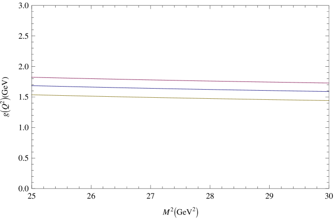
Figure 3: $g^{B_{c}^{PS}}_{h_{b}B_{c}^{V}B_{c}^{PS}}(Q^{2}=5~{}GeV^{2})$ as a function of the Borel mass ${M}^{2}$. The continuum thresholds, $s_{0}=(106.08,108.16,110.25)~{}GeV^{2}$, $s_{0}^{\prime}=(45.3,46.66,48.3)~{}GeV^{2}$ and ${M^{\prime}}^{2}=20~{}GeV^{2}$ are used. The green, blue and purple lines are for minimum central and maximum values of $s_{0}$ and $s_{0}^{\prime}$

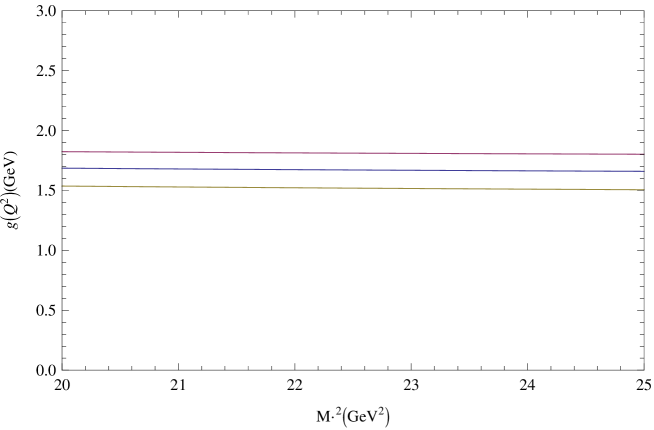
Figure 4: $g^{B_{c}^{PS}}_{h_{b}B_{c}^{V}B_{c}^{PS}}(Q^{2}=5~{}GeV^{2})$ as a function of the Borel mass ${M}^{2}$. The continuum thresholds, $s_{0}=(106.08,108.16,110.25)~{}GeV^{2}$, $s_{0}^{\prime}=(45.3,46.66,48.3)~{}GeV^{2}$ and ${M}^{2}=25~{}GeV^{2}$ are used. The green, blue and purple lines are for minimum central and maximum values of $s_{0}$ and $s_{0}^{\prime}$

Our further numerical analysis shows that the dependence of the form factors on $q^{2}$ with the definite values of auxiliary parameters fits with the following function:

$$g_{h_{b}B_{c}^{V}B_{c}^{PS}}^{i}(Q^{2})=Ae^{BQ^{2}}+C$$ (30)

where $Q^{2}=-q^{2}$, $i$ stands for $B_{c}^{PS}$ and $B_{c}^{V}$ off-shell cases, and the value of $A,~{}B$ and $C$ are shown in Table II.

By definition, the coupling constant is the value of $g_{h_{b}B_{C}^{V}B_{C}^{PS}}^{i}(Q^{2})$ at $Q^{2}=-m_{meson}^{2}$ Rodrigues , where $m_{meson}$ is the mass of the on-shell mesons.

TABLE II. Value of A, B and C for fit function for $B_{c}^{PS}$ and $B_{c}^{V}$ off-shell cases:

$$B_{c}^{V}$$ off-shell off-shell

Substituting $Q^{2}=-m_{B_{c}^{PS}}^{2}$ and $Q^{2}=-m_{B_{c}^{V}}^{2}$ in Eq. (30), the $g_{h_{b}B_{C}^{V}B_{C}^{PS}}^{B_{C}^{PS}}=8.80\pm 2.84GeV^{-1}$ and $g_{h_{b}B_{C}^{V}B_{C}^{PS}}^{B_{C}^{V}}=9.34\pm 3.12GeV^{-1}$ are obtained for $B_{c}^{PS}$ and $B_{c}^{V}$ off-shell cases, respectively. The average value of the $g_{h_{b}B_{C}^{V}B_{C}^{PS}}$ strong coupling constant is found to be

$$g_{h_{b}B_{C}^{V}B_{C}^{PS}}=(9.07\pm 2.93)GeV^{-1}$$ (31)

Note that roughly $80\%$ of the errors in our numerical calculation arise from the variation continuum thresholds in intervals shown in Eqs. (27,28) and 29, and remaining $20\%$ occure as a result of the quark masses when one proceeds from the $\bar{MS}$ to the pole-scheme mass parameters, the input parameters.

In conclusion, we calculate the strong coupling constant $g_{h_{b}B_{C}^{V}B_{C}^{PS}}$ using the three-point QCD sum rules. Our results show that the average value of the strong coupling constant is $g_{h_{b}B_{C}^{V}B_{C}^{PS}}=(9.93\pm 2.7)GeV^{-1}$. Furthermore, the errors in our numerical calculations depend on continuum threshold and variation of the quark masses in different mass schemes.

References

• (1) B. Aubert et al. Phys. Rev. Lett. 101, 071801 (2008).
• (2) I. Adachi et al. [Belle Collaboration], Phys.Β Rev.Β Lett.Β  108, 032001 (2012).
• (3) V. Bashiry, Phys.Β Rev.Β D 84, 076008 (2011).
• (4) M. E. Bracco, A. Cerqueira Jr., M. Chiapparini, A. Lozea, M. Nielsen, Phys. Lett. B 641, 286-293 (2006).
• (5) Z. G. Wang, S. L. Wan, Phys. Rev. D 74, 014017 (2006).
• (6) B.Β Osorio Rodrigues, M.Β E.Β Bracco, M.Β Nielsen and F.Β S.Β Navarra, Nucl.Β Phys.Β A 852, 127 (2011) [arXiv:1003.2604 [hep-ph]].
• (7) F.S. Navarra, M. Nielsen, M.E. Bracco, M. Chiapparini and C.L. Schat, Phys. Lett. B 489, 319 (2000)
• (8) M. E. Bracco, M. Chiapparini, A. Lozea, F. S. Navarra and M. Nielsen, Phys. Lett. B 521, 1 (2001)
• (9) Z. G. Wang, Nucl. Phys. A 796, 61 (2007), Eur. Phys. J. C 52, 553 (2007), Phys. Rev. D 74, 014017 (2006).
• (10) K. Azizi and H. Sundu, J. Phys. G 38, 045005 (2011) [arXiv:1009.5320 [hep-ph]].
• (11) C. Y. Cui, Y.L. Liu and M.Q. Huang, Phys. Rev. D (2012) [arXiv:1210.2789v [hep-ph]].
• (12) A. Cerqueira Jr., B. OsΓ³rio Rodrigues, M.E. Bracco, Nucl. Phys. A 874, 130 (2012).
• (13) Chun-Yu Cui, Yong-Lu Liu, Ming-Qiu Huang, Phys. Lett B707, 129 (2012) and B711, 317 (2012).
• (14) V. A. Fock, Sov. Phys. 12, 404 (1937).
• (15) J. Schwinger, Phys. Rev.82, 664 (1951).
• (16) V. Smilga, Sov. J. Nucl. Phys. 35, 215 (1982).
• (17) J. Beringer et al. (Particle Data Group), Phys. Rev. D86, 010001 (2012).
• (18) Z. G. Wang, Eur.Β  Phys.Β  J.Β A 49, 131 (2013).
• (19) B. L. Ioffe, Prog. Part. Nucl. Phys. 56, 232 (2006).
• (20) E.Β V.Β Veliev, K.Β Azizi, H.Β Sundu and N.Β Aksit, J.Β Phys.Β G 39, 015002 (2012) [arXiv:1010.3110 [hep-ph]].
• (21) W. Lucha, D. Melikhov and S. Simula, Phys. Rev. D 79, 0960011 (2009).