Dynamical Models of Elliptical Galaxies – I. Simple Methods

Abstract

We study dynamical models for elliptical galaxies, deriving the projected kinematic profiles in a form that is valid for general surface brightness laws and (spherical) total mass profiles, without the need for any explicit deprojection. We provide accurate approximations of the line of sight and aperture-averaged velocity dispersion profiles for galaxies with total mass density profiles with slope near $-2$ and with modest velocity anisotropy using only single or double integrals respectively. This is already sufficient to recover many of the kinematic properties of nearby ellipticals.

As an application, we provide two different sets of mass estimators for elliptical galaxies, based on either the velocity dispersion at a location at or near the effective radius, or the aperture-averaged velocity dispersion. In the large aperture (virial) limit, mass estimators are naturally independent of anisotropy. The spherical mass enclosed within the effective radius $R_{\rm e}$ can be estimated as $2.4R_{\rm e}\langle\sigma^{2}_{\rm p}\rangle/G$, where $\langle\sigma^{2}_{\rm p}\rangle$ is the average of the squared velocity dispersion over a finite aperture. This formula does not depend on assumptions such as mass-follows-light, and is a compromise between the cases of small and large apertures sizes. Its general agreement with results from other methods in the literature makes it a reliable means to infer masses in the absence of detailed kinematic information. If on the other hand the velocity dispersion profile is available, tight mass estimates can be found that are independent of the mass-model and anisotropy profile. In particular, for a de Vaucouleurs surface brightness, the velocity dispersion measured at $\approx 1R_{\rm e}$ yields a tight mass estimate (with 10 % accuracy) at $\approx 3R_{\rm e}$ that is independent of the mass model and the anisotropy profile. This allows us to probe the importance of dark matter at radii where it dominates the mass budget of galaxies.

Explicit formulae are given for small anisotropy, large radii and/or power-law total densities. Motivated by recent observational claims, we also discuss the issue of weak homology of elliptical galaxies, emphasizing the interplay between morphology and orbital structure.

1 Introduction

Galaxies are known to contain both luminous and dark matter (DM). In particular, DM haloes provide the seeds of galaxy formation, as baryons cool and fall towards the centres of DM overdensities in protoclusters, resulting eventually in the luminous, directly observable components. Once gas is converted into stars, the assembly of central objects proceeds via mergers (Cattaneo et al., 2011; Johansson et al., 2012).

Cosmological DM-only simulations offer predictions as to the shape, density profile and typical mass of DM haloes (Navarro et al., 1996). However, the buildup of baryonic matter affects the DM haloes in which they assemble, through gravitational interaction between the luminous and dark component. When baryonic effects are included in the simulations, these can transfer energy between the luminous and dark components and alter the DM profile through different channels (Abadi et al., 2010; Di Cintio et al., 2013). In particular, in elliptical galaxies baryonic feedback (Dubois et al., 2013) and virialisation of the infalling material (Lackner & Ostriker, 2010) can produce a shallower density profile, whereas a slow mass build-up tends to steepen it (Blumenthal et al., 1986; Lackner & Ostriker, 2010).

When the assembly of central objects is studied with higher-resolution and smaller-scale simulations, a set of prescriptions must be adopted to quantify the importance of baryonic feedback, amount of substructure and merging rates. These yield distinctive signatures on the final state, in terms of size and mass of the stellar component as well as DM content and density profile (Nipoti et al., 2012; Hilz et al., 2013; Remus et al., 2013).

Then, investigating the DM profiles of observed galaxies provides tests of galaxy formation scenarios. The task is simpler for late-type galaxies, in which the orbits of the stars are generally near-circular. In early-type galaxies, the role of the mass profile in the observed kinematics is degenerate with the orbital distribution of stars. This is commonly known as the mass-anisotropy degeneracy, and constitutes the main obstacle to robust conclusions on the dynamics of elliptical galaxies. Equivalently, only the projected observables (surface brightness and line-of-sight velocities) are available, whereas the dynamics of these systems is characterized by the deprojected, three-dimensional densities and velocities.

The investigation of DM in elliptical galaxies usually relies on techniques that construct three-dimensional models and compare their projected properties to the observational data. This approach is traditionally implemented via the Jeans equations governing the velocity moments of the distribution function, adopting or relaxing the approximation of spherical symmetry (Emsellem et al., 1994; Evans & de Zeeuw, 1994; Cappellari et al., 2006, 2013). A more rigorous alternative considers distribution functions and orbit modelling for the luminous component (Schwarzschild, 1979; Richstone & Tremaine, 1984; Bertin et al., 1994; Evans, 1994; Carollo et al., 1995; Krajnović et al., 2005, and references therein), which has also the advantage of encoding the whole kinematic information beyond the second velocity moments (Merritt & Saha, 1993; Gerhard et al., 1998).

When the kinematic information is averaged over some spatial aperture, such as in integral-field or long-slit spectroscopy of unresolved stellar populations, the importance of orbital structure is reduced. Then, a theoretical framework that naturally encodes aperture-averaging would put the stress on the adopted physical model, rather than on the numerical details that are inherent in, for example, orbit-based descriptions. Within the Jeans formalism in spherical, the projected velocity dispersion $\sigma_{\rm p}$ follows from the density and anisotropy profiles. Mamon & Łokas (2005b) provided expressions of $\sigma^{2}_{\rm p}$ in terms of single integrals of mass profile and luminosity density, for a set of simple anisotropy models. Mamon & Łokas (2005a) reduced the expressions for aperture-averaged velocity dispersions from triple integrals (usually shown in the literature) to single ones in the isotropic case. Here, we develop an approach that operates just within the direct observables, in particular the surface brightness profile rather than the luminosity density. This has already been studied by Agnello et al. (2013) in the context of gravitational lensing by early-type galaxies. In this paper, we extend our earlier formalism to include the role of anisotropy explicitly within different models.

In Section 2, we present new formulae for line of sight and aperture-averaged velocity dispersions. Within the approach followed here, there is no need to perform any explicit or approximate deprojection. Section 3 provides simple explicit results, for scale-free densities or modest anisotropy and/or large radii. We compare our findings to empirical aperture corrections that are commonly used elsewhere. We show that some structural properties (such as kinematic profiles and typical masses, Figs 2 and  6) of early-type galaxies can be understood by means of simple models, perhaps even deceptively simple! In Section 4, we present different mass estimators based on our formalism and we characterise the possible sources of error. We sum up our conclusions in Section 5. The methods illustrated below are particularly useful in the presence of noisy data (e.g. Paper II in this series) or poor spatial resolution of the measured kinematics.

2 Line-of-sight Kinematics

2.1 Preliminaries

We consider spherical models, such that the velocity dispersion tensor is diagonal in spherical coordinates $(r,\theta,\phi)$ and the only distinction is between radial and tangential motions. Let the anisotropy profile be written as

$$\beta(r)=1-\frac{\langle v_{\theta}^{2}+v_{\varphi}^{2}\rangle}{2\langle v_{r}^{2}\rangle}\ .$$ (1)

Then, the Jeans equation for supporting the stellar component with luminosity density $\nu$ in a gravitational potential $\Phi$ is

$${\partial(\nu\langle v_{r}^{2}\rangle)\over\partial r}+\frac{2\beta\nu\langle v_{r}^{2}\rangle}{r}=-\nu{\partial\Phi\over\partial r}.$$ (2)

Our models are stationary ($\partial_{t}\nu=\partial_{t}\Phi=0$), with neither radial flows ($\langle v_{r}\rangle=0$) nor Hubble flow. While this hypothesis is acceptable for the internal dynamics of elliptical galaxies, the application of the Jeans equations to galaxy clusters requires additional correction terms (Falco et al., 2013).

Using the shorthand

$$J_{\beta}(r,s)=\exp\left[{\int_{r}^{s}2\beta(r^{\prime})\mathrm{d}r^{\prime}/r^{\prime}}\right]$$ (3)

for the integrating factor, eq. (2) is easily solved for the radial velocity dispersion (e.g., van der Marel, 1994; An & Evans, 2011)

$$\langle v_{r}^{2}\rangle=\frac{G}{\nu(r)}\int_{r}^{\infty}\frac{M(s)\nu(s)}{s^{2}}J_{\beta}(r,s)\mathrm{d}s\ ,$$ (4)

where we have cast the radial force in terms of the enclosed mass $M(r).$ Observations provide the projected velocity second moment $\sigma_{\rm p}(R)$ at radius $R,$ which is given by

$$\Sigma\sigma_{\rm p}^{2}(R)=2\int_{R}^{\infty}\left(1-\beta(r)\frac{R^{2}}{r^{2}}\right)\frac{\nu(r)\langle v_{r}^{2}\rangle r\mathrm{d}r}{\sqrt{r^{2}-R^{2}}}$$ (5)

(Binney & Mamon, 1982), where $\Sigma(R)$ is the surface brightness. The luminosity density can be obtained from the surface brightness profile via Abel deprojection,

$$\nu(r)=-\frac{1}{\pi}\int_{r}^{\infty}\frac{\partial_{R}(\Sigma(R))\mathrm{d}R}{\sqrt{R^{2}-r^{2}}}\ ,$$ (6)

and inserted in eq. (5). However, it can be useful to have results that depend directly on the surface brightness profile, without the need for explicit deprojection, integration of the Jeans equations and re-projection. This contrasts with other methods, which rely on numerical or approximate deprojections of fitting profiles, and therefore is the subject of the following sections.

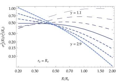
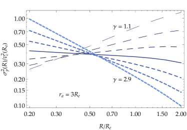
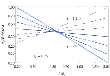
Figure 1: Profiles of squared projected velocity dispersion $\sigma^{2}_{\rm p}(R)$ rescaled to squared circular velocity $v^{2}_{\rm c}(R_{\rm e}),$ as a function of $R/R_{\rm e}$. Here, $\Sigma(R)$ is a de Vaucouleurs profile, the total density is $\rho_{\rm tot}\propto r^{-\gamma}$ and the anisotropy profile is of Osipkov-Merritt form (eq. 11 with $\beta_{\infty}=1$). The density exponent varies in steps of 0.3 between 1.1 (long-dashed, darkest, thinnest lines, labeled) to 2.9 (shortest-dash, clearest, thickest lines, labeled); full lines mark the flat rotation curve case of $\gamma=2.$ Different panels correspond to different values of anisotropy radius $r_{\rm a}$ as in the legends. Top: $r_{\rm a}=R_{\rm e};$ middle: $r_{\rm a}=3R_{\rm e};$ bottom: $r_{\rm a}=10R_{\rm e}.$ Pinch points, at which dependence on the adopted mass model is minimised, are present in each panel, but the location changes with anisotropy.

2.2 Line of Sight Velocity Dispersion Profiles

Inserting eq. (4) in eq. (5), and exchanging the orders of integration, an integration by parts leads to

$$\Sigma\sigma^{2}_{\rm p}(R)=2G\int_{R}^{\infty}\frac{\nu(r)M(r)}{r^{2}}\left(\sqrt{r^{2}-R^{2}}+k_{\beta}(R,r)\right)\mathrm{d}r\ ,$$ (7)

where

$$k_{\beta}(R,x)=\int_{R}^{x}\frac{(2r^{2}-3R^{2})\beta(r)J_{\beta}(r,x)}{r\sqrt{r^{2}-R^{2}}}\mathrm{d}r\ .$$ (8)

The kernel $k_{\beta}(R,x)$ has already been expressed in analytical form by Mamon & Łokas (2005b) for some particular choices of the anisotropy profile. Eq. (7) gives the line-of-sight velocity dispersion as a function of projected radius $R$. The dependence on $\beta$ is separated out in the second integral on the right-hand side. We can re-arrange this result explicitly in terms of the observable stellar surface brightness $\Sigma$. First, we note the useful identity

$$\frac{\mathrm{d}}{\mathrm{d}y}\int_{R}^{y}\frac{f(x,R)x}{\sqrt{y^{2}-x^{2}}}\mathrm{d}x=y\int_{R}^{y}\frac{\partial_{x}f(x,R)}{\sqrt{y^{2}-x^{2}}}\mathrm{d}x\ ,$$ (9)

which holds true if and only if $f(R,R)=0$ and provided the integrals are well defined. Here, and elsewhere in this section, we defer the technical details of proofs to Appendix A for the interested reader. Inserting eq. (6) in eq. (7), integrating by parts and exploiting eq (9), we get in the end

$$\Sigma\sigma_{\rm p}^{2}(R)=\frac{2G}{\pi}\int_{R}^{\infty}s\Sigma(s)\int_{R}^{s}\frac{\partial_{r}\left(M(r)\sqrt{r^{2}-R^{2}}/r^{3}\right)}{\sqrt{s^{2}-r^{2}}}\mathrm{d}r\mathrm{d}s\$$

$$+\frac{2G}{\pi}\int_{R}^{\infty}s\Sigma(s)\int_{R}^{s}\frac{\partial_{r}\left(M(r)k_{\beta}(R,r)/r^{3}\right)}{\sqrt{s^{2}-r^{2}}}\mathrm{d}r\mathrm{d}s\ .$$ (10)

This gives the line of sight velocity dispersion in terms of the observable $\Sigma$ as well as model parameters such as the mass $M(r)$ and anisotropy profile $\beta(r)$. It replaces the three equations (4)-(6), generalises equations (A15) and (A16) of Mamon & Łokas (2005b) and obviates the need for explicit projections and deprojections (Mamon & Łokas, 2005b, in eq. A8). Isotropic models ($\beta=0$) are all encoded in the first line, whilst the second gives corrections for anisotropic models ($\beta\neq 0$).

To make further progress, it is useful to introduce a two-parameter family of anisotropy profiles

$$\beta(r)=\beta_{\infty}\frac{r^{2}}{r^{2}+r_{\rm a}^{2}}\ .$$ (11)

This class of models allows us to examine systems where the anisotropy changes gradually from isotropy at the center to a limiting value of $\beta_{\infty}$ at large radii, as well as cases where the anisotropy is fixed at a uniform value ($r_{\rm a}\rightarrow 0$). The integrating factor is simply

$$J_{\beta}(r,s)=\left(\frac{s^{2}+r_{\rm a}^{2}}{r^{2}+r_{\rm a}^{2}}\right)^{\beta_{\infty}}$$ (12)

(see Mamon et al., 2013, for the expression of $J_{\beta}$ for other anisotropy models). Although we will return to the generalised form  (11) in Section  3, for the moment let us set $\beta_{\infty}=1$ so that the models are strongly radially anisotropic at large radii. Note that this corresponds to the ansatz introduced by Osipkov (1979) and Merritt (1985).

To gain insight, let us start with scale-free total densities, $\rho_{\rm tot}\propto r^{-\gamma}.$ This choice is appropriate for elliptical galaxies, at least within a few effective radii (Treu & Koopmans, 2004; Mamon & Łokas, 2005b; Gavazzi et al., 2007; Humphrey & Buote, 2010). Fig. 1 shows the typical behaviour of $\sigma_{\rm p}^{2}$ as a function of $R,$ for a de Vaucouleurs luminous profile in different scale-free total densities, having the same enclosed mass at the effective radius $R_{\rm e}.$ The line-of-sight velocity dispersion has been normalised to the circular velocity $v_{\rm c}(R_{\rm e})$ at the effective radius to highlight the contribution from the mass profile rather than from overall normalisations. Models with $\gamma>2$ have a falling rotation curve and a declining velocity dispersion at all radii. When $\gamma<2$ the velocity dispersion increases at small radii and decreases slowly at large radii. The transition between these two behaviours happens around $\gamma\approx 2$ (i.e. a flat rotation curve), although the velocity dispersion profile is not exactly flat. The exact value of the transition exponent, where $\sigma_{p}(R)$ is almost uniform, varies depending on the structural properties (e.g. Sérsic index and anisotropy).

More important than the shape of single velocity dispersion profiles is the existence, for each chosen anisotropy, of a pinch radius $R_{\sigma}$ where any dependence on the mass model is minimal (Mamon & Boué, 2010; Wolf et al., 2010). This location changes with anisotropy $\beta$ (c.f., Fig.1) and with the Sérsic index. In particular, steeper profiles (lower Sérsic indices) produce a smaller variation in $R_{\sigma}$ with $\beta.$ This fact can be justified in the light of asymptotic behaviours at small $\beta$ or large radii, which are discussed in Section 3; we will exploit that in Section 4.1 to construct a family of mass estimators.

The behaviour of $\sigma_{\rm p}(R)$ with the effective radius is controlled essentially by the circular velocity. If $R_{\rm e}$ is increased, the overall normalisation decreases for $\gamma>2$ (as $v_{\rm c}(R_{\rm e})\propto R_{\rm e}^{1-\gamma/2}$) and increases for $\gamma<2.$ This means that, for a rising (declining) circular velocity curve, increasing the effective radius will increase (decrease) the overall magnitude of the velocity dispersion at fixed $R/R_{\rm e}.$ This phenomenon is clear within scale-free total densities and uniform anisotropy because, in this case, the only available lengthscale is $R_{\rm e}$ and so we can expect $\sigma^{2}_{\rm p}(R)$ to be modulated by $GM(R_{\rm e})/R_{\rm e}=R_{\rm e}^{2-\gamma}$ (see, for example, Dekel et al., 2005, who give the exact solutions for scale-free tracers in scale-free total densities).

More elaborate mass models, exhibiting different power-law regimes in different regions, can be understood in terms of the kinematic profiles shown here. For example, a Navarro-Frenk-White density $\rho_{\rm tot}\propto r^{-1}(1+r/r_{\rm s})^{-2}$ produces a line of sight dispersion profile that is approximated by the one with $\gamma\approx 1$ at small radii and $\gamma\rightarrow 3$ at large radii, provided $\Sigma(R)$ declines fast enough with $R.$ However, in most cases, eq. (10) allows for an analytic evaluation of the inner integral giving the mass-kernel, without any need for the approximation of scale-free total densities.

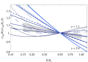
Figure 2: Line-of-sight velocity dispersion, averaged over an aperture of radius $R,$ as a function of $R/R_{\rm e}$ for a de Vaucouleurs luminosity profile in scale-free total mass densities, with exponent $\gamma$ ranging in steps of 0.3 from 1.1 (darkest, thinnest lines, labeled) to 2.9 (lightest, thickest lines, labeled). The curves are computed using eq. (2.3). Every profile has been rescaled to the aperture-averaged velocity dispersion within $R_{\rm e}/2.$ Full lines: Osipkov-Merritt anisotropic models with $\beta(R_{\rm e})=1/2;$ dashed lines: isotropic models. The grey-shaded region shows the empirical relation $\sigma_{\rm ap}(R)\propto R^{-b},$ with $b=0.066\pm 0.034$ (Cappellari et al. 2006).

2.3 Aperture-averaged Velocity Dispersions

In practice, kinematics are measured over some aperture and blurred by a point-spread function. Then, the quantity to be compared to observations is the radial average

$$\sigma^{2}_{\rm ap}(R)\equiv\frac{2\pi\int_{0}^{R}s\Sigma(s)\sigma_{\rm p}^{2}(s)\mathrm{d}s}{L(R)}\ ,$$ (13)

with

$$L(R)=2\pi\int_{0}^{R}s\Sigma(s)\mathrm{d}s\$$ (14)

being the projected luminosity within $R.$ Averages within radial annuli or slits can be derived from these formulae by means of straightforward manipulations.

The triple integrals can be rearranged to express the aperture-averaged velocity dispersion as a sum of three terms (see Appendix A)

$$\sigma^{2}_{\rm ap}(R) = \frac{4\pi G}{3L(R)}\left(\int_{0}^{\infty}M(r)\nu(r)r\mathrm{d}r\right.$$

$$- \int_{R}^{\infty}M(r)\nu(r)\frac{(r^{2}-R^{2})^{3/2}}{r^{2}}\mathrm{d}r$$

$$+ 3\left.R^{2}\int_{R}^{\infty}\frac{M(r)\nu(r)}{r^{2}}Z_{\beta}(R,r)\mathrm{d}r\right)\$$

where we have used the shorthand

$$Z_{\beta}(R,y)=\int_{R}^{y}J_{\beta}(r,y)\beta(r)\sqrt{r^{2}-R^{2}}{\mathrm{d}r\over r}\$$ (16)

The first line gives the virial limit, the second one provides aperture corrections for $\beta=0$, while the third one expands to the case of anisotropy $\beta\neq 0$. Without the third line, this equation is equivalent to the isotropic results of Mamon & Łokas (2005b). For computational purposes, it is useful to replace the stellar density $\nu$ in eq. (2.3) with the stellar surface brightness $\Sigma$ to obtain

$$\sigma^{2}_{\rm ap}(R) = \frac{4G}{3L(R)}\left[\int_{0}^{\infty}\Sigma(s)s\int_{0}^{s}\frac{4\pi\rho_{\rm tot}(r)r^{2}}{\sqrt{s^{2}-r^{2}}}\mathrm{d}r\mathrm{d}s\right.$$

$$- \int_{R}^{\infty}\Sigma(s)s\int_{R}^{s}\frac{\partial_{r}\left(M(r)(r^{2}\!-\!R^{2})^{3/2}/r^{3}\right)}{\sqrt{s^{2}\!-\!r^{2}}}\mathrm{d}r\mathrm{d}s$$

$$+ \left.3R^{2}\int_{R}^{\infty}\Sigma(s)s\int_{R}^{s}\frac{\partial_{r}\left(M(r)Z_{\beta}(R,r)/r^{3}\right)}{\sqrt{s^{2}\!-\!r^{2}}}\mathrm{d}r\mathrm{d}s\right]$$

The aperture-averaged velocity dispersion $\sigma^{2}_{\rm ap}(R)$ is the outcome of two factors. The first is the mass model: as expected, higher masses correspond to higher velocity dispersions at fixed effective radius $R_{\mathrm{e}}.$ The second is the anisotropy, which enters only in the last term of eq (2.3) and whose effect on the velocity dispersion has the same sign as $\beta$. This means that the uncertainties on the mass modelling due to observational errors on the measured velocity dispersions can be decoupled from the systematic uncertainties that are encoded in $\beta$ (e.g. Koopmans et al., 2009; Agnello et al., 2013). The same remarks hold here for the overall mass normalisation and behaviour with $R_{\rm e}.$

Fig. 2 shows the behaviour of aperture-averaged velocity dispersions $\sigma^{2}_{\rm ap}(R)$ scaled to the values at ${R_{\rm e}}/{2}$ in two cases – namely, an Osipkov-Merritt profile with $\beta(R_{\rm e})=\tfrac{1}{2}$ and an isotropic model with $\beta=0$ everywhere. The choice of $R_{\rm e}/2$ is used solely to make comparisons with other work (Cappellari et al., 2006) more immediate.

In general, models with $\gamma\lesssim 2$ predict an averaged velocity dispersion with a minimum at aperture radii between $R_{\rm e}/3$ and $R_{\rm e}/2,$ increasing at both small and large apertures, whereas steeper models produce a monotonically decreasing profile. The median of the grey-shaded region in Fig. 2, corresponding to the empirical relation $\sigma^{2}_{\rm ap}(R)\propto R^{-0.066}$ (Cappellari et al., 2006), is hardly distinguishable from a model with a de Vaucouleurs luminous profile, a perfectly flat rotation curve and $\beta=0.$ Models with $\beta(R_{\rm e})=\tfrac{1}{2}$ (full lines) require slightly steeper density profiles to fit the grey band, approximately $\gamma=2.1\pm 0.1$. This small modulation of $\gamma$ with anisotropy suggests that, over lengthscales that are comparable to the effective radius, nearby elliptical galaxies show weak homology – in the sense that their dynamical properties are consistent with a total density scaling like $r^{-2}$ and just modest radial anisotropy.

However, the median behaviour at radii $R_{\rm e}/2\lesssim R\lesssim R_{\rm e}$ is not necessarily indicative of the density profile of single systems, especially over larger lengthscales. Analysis of the hot X-ray gas in early-type galaxies by Humphrey & Buote (2010) supports the approximation of a scale-free total mass profile out to large radii, but the relative exponent varies appreciably over their sample. Koopmans et al. (2009) studied the density exponent $\gamma$ in 58 galaxies in the SLACS sample (Bolton et al., 2006). The typical density exponent from gravitational lensing, estimated by means of global scaling relations over the whole sample, is in the interval $\gamma_{l}=(2.03\pm 0.07).$ On the other hand, on a galaxy-by-galaxy basis the most likely density exponents occupy a much wider range, with larger intrinsic uncertainties. The behaviour of $\gamma$ in individual galaxies and the mean exponent $\gamma_{l}$ derived by scaling relations over the whole sample are not directly related to one another. Then, considerable care should be taken when the dynamics of individual galaxies is studied, as to avoid the ecological fallacy of exporting ensemble correlations at the individual level. If the DM content at large radii is studied, simple analyses enforcing $\gamma\approx 2$ may bias the inferred DM masses, automatically favouring the values resulting from a flat rotation curve.

The kinematic and photometric properties of individual galaxies can deviate appreciably from the simple, average behaviour illustrated above. In fact, the collection of profiles shown in Cappellari et al. (2006), if interpreted in terms of the models shown in Fig. 2, spans the whole range $1\lesssim\gamma\lesssim 3$ and $r_{\rm a}\gtrsim R_{\rm e}.$ In general, there is no guarantee that individual systems are isotropic or that $\gamma=2$. Moreover, the morphology of individual galaxies can vary within the Sérsic family of profiles (de Vaucouleurs, 1948; Sersic, 1968)

$$\Sigma(R)=\Sigma_{0}\ \mathrm{exp}\left[-b_{n}(R/R_{\rm e})^{1/n}\right]\ ,$$ (18)

where $b_{n}$ is defined such that $R_{\rm e}$ encloses half of the total luminosity. A convenient expression of $b_{n}$ in $n$ has been provided by Ciotti & Bertin (1999). The light profiles of some elliptical galaxies can be better fitted by Sérsic models with an index substantially different from the de Vaucouleurs value $n=4.$ That said, the assumption of weak homology can be taken as a first approximation to infer properties of the mass profile within $R_{\rm e},$ before more detailed analyses are undertaken.

3 Asymptotic Results

3.1 Line of Sight Velocity Dispersion Profiles

A convenient aspect of the Jeans formalism is that eqs (4) and (5) involve information only from radii larger than the upper limits of integration (see e.g., van der Marel, 1994; Mamon & Łokas, 2005b). In particular, if the stellar density decays fast enough (which is always the case for elliptical galaxies in practice), the dominant contribution to the integrals is from radii just slightly greater than the lower extremes of integration. This turns out to be useful in practice when handling the effects of anisotropy, since we just need to consider the anisotropy profile and the mass $M(r)$ near the radii of interest.

We will now analyse some applications of eq. (10). To this end, we return to the generalisation of the Osipkov-Merritt anisotropy profile given in eq (11). With this choice of $\beta$, the kernel $k_{\beta}$ is:

$$k_{\beta}(R,r) = -\beta(R)\left(\frac{r_{\rm a}^{2}+r^{2}}{r_{\rm a}^{2}+R^{2}}\right)^{\beta_{\infty}}\sqrt{r^{2}-R^{2}}$$ (19)

$$\times \left[F\left(\frac{1}{2},z\right)+\frac{2(1-r^{2}/R^{2})}{3}F\left(\frac{3}{2},z\right)\right]\ ,$$

where $z=(R^{2}-r^{2})/(r_{\rm a}^{2}+R^{2})$ and $F(a,z)$ is the hypergeometric function ${}_{2}F_{1}\left(a,1+\beta_{\infty},a+1,z\right).$ Appendix B lists the special cases of $\beta_{\infty}=1,\tfrac{1}{2}$ and $r_{\rm a}=0$.

For any surface brightness law, the kinematic profile is given by a double integral where $\Sigma(R)$ is modulated by a kernel that depends just on the potential chosen. The function $k_{\beta}$ can be expanded in powers of $(r^{2}-R^{2})^{1/2}$ and the expansion to first order is

$$k_{\beta}(R,r)\ \sim\ -\beta(R)\sqrt{r^{2}-R^{2}}+...\ .$$ (20)

If $\nu(r),$ and hence $\Sigma(R),$ decay fast enough with radius $R,$ the next orders in the expansion can be neglected in a first approximation. If this is the case, the kinematic profile can be obtained by neglecting the second line in eq. (10) and multiplying the first line by $1-\beta(R).$ This is useful for obtaining asymptotic results at small and large radii.

An interesting class of results at small and large radii is provided by scale-free densities, $\rho_{\rm tot}(r)=\rho_{0}(r/r_{0})^{-\gamma}.$ At small radii, we can rely on the hypothesis of mild anisotropy. First, observations of nearby elliptical galaxies (Gerhard et al., 2001; Cappellari et al., 2006) show little or no departure from isotropy inside $R_{\rm e}.$ Second, just a mild degree of anisotropy is generally allowed in these systems by reasons of physical consistency (Ciotti et al., 2009). This means that (see Appendix A for details)

$$\frac{\Sigma(R)\sigma_{\rm p}^{2}(R)}{1\!-\!\beta(R)}=\frac{4\pi G\rho_{0}r_{0}^{\gamma}}{3\!-\!\gamma}\int_{R}^{\infty}s^{1-\gamma}\Sigma(s)g_{\rm p}\left({R\over s},\gamma\right)\mathrm{d}s\ ,$$ (21)

where

$$g_{\rm p}(x,\gamma)=\frac{1}{\pi}\int_{x^{2}}^{1}\frac{t^{-\gamma/2-1}\left[(1-\gamma)t+\gamma x^{2}\right]}{\sqrt{t-x^{2}}\sqrt{1-t}}\mathrm{d}t\ .$$ (22)

The kernel $g_{\rm p}$ can be expressed as a combination of hypergeometric functions and can be easily expanded in powers of $x$. An excellent approximation for $x\lesssim 1$ is

$$g_{\rm p}(x,\gamma) \sim \ 1+{\gamma\over 2}(x-1)+{\gamma\over 8}\left(1-{\gamma\over 2}\right)(x-1)^{2}$$ (23)

$$+ \frac{\gamma^{2}(\gamma^{2}-4)}{96}(x-1)^{3}\ .$$

The result $g_{\rm p}=x$ for $\gamma=2$ (flat rotation curve) is exact.

At large radii, we cannot necessarily assume $|\beta|\ll 1.$ However, we can approximate the kernel in the integrals for $y\gtrsim R$ as done above in eq. (20). Higher orders only become important for high values of $y,$ where the integrand is suppressed by the declining $\Sigma(y).$ Also, we can use the asymptotic limit $\beta\rightarrow\beta_{\infty}$ for the anisotropy profile. For $r\gg R,$ the kernel $k_{\beta}$ grows at most linearly with $r$ (which happens when $\beta_{\infty}=1$). For $\beta\sim\beta_{\infty}$ and $r\gtrsim R$, we have

$$\frac{k_{\beta}(R,r)}{\beta_{\infty}R}\ \sim\ -\left[1-\left(1-\tfrac{2}{3}\beta_{\infty}\right)\delta^{2}+\tfrac{3}{5}\left(1-\tfrac{2}{3}\beta_{\infty}\right)^{2}\delta^{4}\right]\delta+...$$ (24)

where $\delta=\sqrt{r^{2}/R^{2}-1}.$ This allows us to write $\sigma_{\rm p}^{2}$ at large radii as a single quadrature involving the tracer density $\nu,$ the mass profile $M$ and a sum of elementary functions (cf Mamon & Łokas, 2005b). Alternatively, the result can be stated in terms of the surface brightness, exploiting eq. (9) in the same manner as done to derive eq. (10).

In particular, for scale-free total densities, the velocity dispersion profile at large radii is asymptotically

$$\Sigma(R)\sigma_{\rm p}^{2}(R)\ \sim \frac{4\pi G\rho_{0}r_{0}^{\gamma}}{3\!-\!\gamma}\int_{R}^{\infty}s^{1-\gamma}\Sigma(s)\left[(1\!-\!\beta_{\infty})g_{\rm p}\left({R\over s},\gamma\right)\right.$$ (25)

$$+ \left.\beta_{\infty}\left(1\!-\!\tfrac{2}{3}\beta_{\infty}\right)h_{\rm p}\left({R\over s},\gamma\right)\right]\mathrm{d}y\ ,$$

with

$$h_{\rm p}(x,\gamma)=\frac{x^{-2}}{\pi}\int_{x^{2}}^{1}\frac{t^{-\gamma/2-1}\sqrt{t-x^{2}}[\gamma x^{2}+(3-\gamma)t]}{\sqrt{1-t}}\ \mathrm{d}t\ ,$$ (26)

having retained just the two terms in equation (24). The kernel $h_{\rm p}$ can be expanded as

$$h_{\rm p}\sim\ \begin{cases}\frac{\displaystyle\Gamma\left((3-\gamma)/2\right)}{\displaystyle\sqrt{\pi}\Gamma\left(2-\gamma/2\right)}\left((3-\gamma)x^{-2}-3(1-\gamma/2)\right)\\ \qquad\qquad\qquad+\mathcal{O}(x^{3-\gamma}),&x\ll 1\\ \\ 3(1\!-\!x)\!-\!\frac{3}{4}(-6\!+\!\gamma)(1-x)^{2}\\ \qquad\qquad\qquad-\frac{\displaystyle 96-\gamma(14+\gamma)}{\displaystyle 16}(1-x)^{3},&x\lesssim 1.\end{cases}$$

In the important flat rotation curve case ($\gamma=2$), the result

$$h_{\rm p}(x,2)=x^{-2}\left(1-x^{3}\right)$$ (27)

holds at all orders.

3.2 Aperture-averaged Velocity Dispersions

For small anisotropy or large aperture radii, eq. (2.3) admits a simple approximation – namely, we may again suppress the third addendum and multiply the second one by $1-\beta(R)$. As a check on our working, we note that for large values of aperture radius $R$, we must recover the virial limit exploited elsewhere (Agnello & Evans, 2012a, b).

We again derive the results for mildly anisotropic systems in scale-free total densities. Starting with eq. (2.3), using the approximation for small $\beta$ and exchanging orders of integration as before, we obtain:

$$\sigma^{2}_{\rm ap}(R)=\frac{16\pi G\rho_{0}r_{0}^{\gamma}}{3(3-\gamma)L(R)}\times\left(k_{\rm ap}(0,\gamma)\int_{0}^{\infty}\Sigma(s)s^{3-\gamma}\mathrm{d}s\right.\$$

$$-\left.(1-\beta(R))\int_{R}^{\infty}\Sigma(s)s^{3-\gamma}k_{\rm ap}(R/s,\gamma)\mathrm{d}s\right)$$ (28)

(cf Agnello et al. 2013). Again, the kernel

$$k_{\rm ap}(x,\gamma)=(4-\gamma)\int_{x}^{1}\sqrt{\frac{u^{2}-x^{2}}{1-u^{2}}}u^{3-\gamma}\mathrm{d}u$$

$$+(\gamma-1)x^{2}\int_{x}^{1}\sqrt{\frac{u^{2}-x^{2}}{1-u^{2}}}u^{1-\gamma}\mathrm{d}u$$ (29)

can be easily expanded in powers of $x:$

$$k_{\rm ap}(x,\gamma)\sim\begin{cases}\frac{\displaystyle\sqrt{\pi}\Gamma((5-\gamma)/2)}{\displaystyle\Gamma(2-\gamma/2)}\times\left[1-\frac{\displaystyle(1-\gamma/2)x^{2}}{\displaystyle 1-\gamma/3}\right.&\\ \left.\qquad\qquad\qquad\quad-\frac{\displaystyle\gamma(1-\gamma/2)x^{4}}{\displaystyle 4(1-\gamma/3)}\right]&x\ll 1,\\ &\\ \frac{\displaystyle 3\pi}{\displaystyle 2}(1-x)-\frac{\displaystyle 3\pi}{\displaystyle 8}(2+\gamma)(1-x)^{2}&\\ \qquad\qquad\qquad\quad+\frac{\displaystyle\pi\gamma(10-\gamma)}{\displaystyle 32}(1-x)^{3}&x\lesssim 1.\end{cases}$$ (30)

The result

$$k_{\rm ap}(x,2)=\frac{\pi}{2}(1-x^{3})$$ (31)

is exact. As a specific example, when we use the anisotropy law (11), we find that our simple asymptotic approximation is excellent for $r_{\rm a}\gtrsim 3R_{\rm e}$. In fact, provided the models are reasonably close to the flat rotation curve case ($1.5\lesssim\gamma\lesssim 2.5$), it performs remarkably well even when $r_{\rm a}=R_{\rm e}$.

The trick for reducing the eqs (10) and  (2.3) for the line of sight and aperture-averaged velocity dispersions is of wider applicability. In each case, the integrals over stellar surface density and total mass are greatly simplified with little loss of accuracy when the anisotropy dependent term is discarded and the previous term multiplied by $1-\beta(R)$. The same trick can also be applied to eqs (7) and (2.3) for which the integrals are written in terms of the stellar density and total mass, if so desired. This then gives single integrals to express both line of sight and aperture-averaged velocity dispersions for arbitrary velocity anisotropy profiles, generalising results obtained by Mamon & Łokas (2005a, b) in special cases.

Finally, we give in Appendix B formulae for the line of sight and aperture-averaged velocity dispersion valid for small anisotropy and/or large radii without the assumption of power-law densities. The formulae are simpler than eqs (10) and  (2.3), as they involve just the total density $\rho_{\rm tot}$ and integrals over the surface brightness $\Sigma$.

4 Mass estimators

In the previous sections, we have seen how the line of sight kinematics can be computed, starting from the mass profile $M(r)$ and a choice of anisotropy profile $\beta.$ Now we ask a complementary question: given the measured kinematics, what is the best inference that we can make on the mass profile?

The dimensional scaling $\sigma^{2}_{\rm p}\propto GM/R$ between the second moment of line of sight velocities, enclosed mass and size is evident in the Jeans formalism (e.g. eqs 10 and 2.3). The inverse passage from $\sigma^{2}_{\rm p}(R)$ to $M(r)$ is possible when $\beta(r)$ is given and the kinematic profile is measured with sufficient accuracy (Mamon & Boué, 2010). However, these conditions are hardly satisfied in practice. Also, observational data are often not sufficient to constrain all the parameters in the mass profile. So, the problem of relating the measured kinematics to mass estimates is often simplified to finding relations of the kind

$$\frac{GM({R_{\rm M}})}{{R_{\rm M}}}\ \equiv v_{\rm c}^{2}({R_{\rm M}})\ =\ {K}\sigma^{2}({R_{\sigma}}),$$ (32)

such that any model-dependence is minimal at the locations ${R_{\sigma}},{R_{\rm M}},$ while the parameter ${K}$ is to be determined. Here, $\sigma^{2}(R)$ could be either the line of sight velocity second moment (eq. 10) or the one averaged inside an aperture of radius $R$ (eq. 2.3), whilst $v_{\rm c}(R)$ denotes the circular velocity at radius $R.$

This issue has been already tackled in a piecemeal manner in the literature. Illingworth (1976) derived a formula for constant mass-to-light ratio models with a de Vaucouleurs profile. The total mass $M$ is

$$M(\infty)\approx{8.5R_{\rm e}\over G}\langle\sigma^{2}_{\rm p}\rangle\ ,$$ (33)

where $\langle\sigma^{2}_{\rm p}\rangle$ is the average value of the squared line of sight velocity dispersion.

Cappellari et al. (2006) studied 25 galaxies in the SAURON survey (Bacon et al., 2001), by means of Jeans equations and orbit-based models. Their analyses suggest a general trend

$$M(\infty)\approx{5R_{\rm e}\over G}\sigma^{2}_{\rm ap}(R_{\rm e})\ ,$$ (34)

where again $M(\infty)$ is the total mass and $\langle\sigma^{2}_{\rm p}\rangle(R_{\rm e})$ is the luminosity-weighted average over one effective radius. The formula holds if there is a negligible DM fraction within the effective radius or, alternatively, if the light traces mass. Cappellari et al. (2006) argued that accounting for an extended DM halo would change the proportionality coefficient in eq. (34) by $\approx 12\%$. This result is calibrated against diverse, high spatial-resolution kinematic profiles (out to $R_{\rm e}$), but its simplicity makes it useful for application to galaxies for which any kinematic information is not as rich. However, the main drawback of eqs (33) and (34) is the assumption of a mass-follows-light hypothesis is not generally satisfied (Treu & Koopmans, 2004; Humphrey & Buote, 2010). Cappellari et al. (2013) revisited the previous analysis on a new set of galaxies with an expanded dataset of spatially resolved kinematics, introducing different models with luminous and dark components. They claim:

$$M(R_{\rm e})\approx{2.5R_{\rm e}\over G}\sigma^{2}_{\rm ap}(R_{\rm e})\ ,$$ (35)

which would be essentially the same result as before if light traced mass.

Analogous formulae have been derived for DM-dominated systems – though the focus has been on dwarf spheroidal galaxies (dSphs), rather than ellipticals. For a dSph with a Plummer luminosity profile and a flat line of sight velocity dispersion $\sigma_{\rm p}$, Walker et al. (2009) showed that the mass within the effective radius is

$$M(R_{\rm e})\approx{2.5R_{\rm e}\over G}\sigma^{2}_{\rm p}.$$ (36)

In particular, Walker et al. (2009) argued from Jeans solutions that the mass within the half-light radius is robust against changes in the velocity anisotropy and halo profiles. Wolf et al. (2010) discovered a different, but related, formula in which ${R_{\rm M}}$ is the radius of the sphere enclosing half of the total light $r_{1/2}$, whilst the velocity dispersion is averaged over large radii

$$M(r_{1/2})\approx\frac{3r_{1/2}\langle\sigma^{2}_{p}\rangle_{\infty}}{G}\ .$$ (37)

They provided a theoretical justification, based on the Jeans equations under the hypothesis that the velocity dispersion profile is approximately flat. Amorisco & Evans (2011) extended this idea by looking for masses robust against variation in the concentration and form of the DM halo profile, using a particular class of distribution functions. They advocated the formula

$$M(1.7R_{\rm e})\approx{5.8R_{\rm e}\over G}\sigma^{2}_{\rm p}(R_{\rm e}),$$ (38)

and so found that the mass enclosed within $r=1.7R_{\rm e}$ was best constrained. A similar approach was pursued by Churazov et al. (2010); there, the $\sigma_{\rm p}$ profiles of Sérsic tracers with a flat rotation curve ($\gamma=2$) were studied, with particular emphasis on isotropic, completely radial or completely tangential stellar orbits, to identify the location where any dependence on anisotropy is minimised. Using the assumption that the total density profile is $\rho\sim r^{-2}$ enabled them to find fully analytical results.

All these formulae share a common ancestry, though they apply to different luminosity profiles and dark halo laws. They all relate the mass enclosed at a specific radius ${R_{\rm M}}$ with the velocity dispersion either at, or averaged within, a particular radius ${R_{\sigma}}$ based on different choices for the distribution function of the stellar populations. Here, we will show how the results of Section 2 can be used systematically to construct mass estimators tailored for elliptical galaxies with Sérsic profiles.

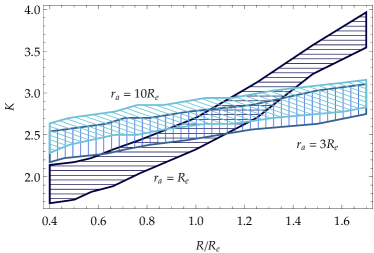
Figure 3: The coefficient ${K}=v_{\rm c}^{2}({R_{\rm M}})/\sigma^{2}_{\rm p}(R)$ versus radius $R$ for a de Vaucouleurs luminous profile in scale-free total densities, with Osipkov-Merritt anisotropy and radii $r_{\rm a}/R_{\rm e}=1,3,10$ (from the most to the least steep sequences). At each value of $R/R_{\rm e},$ a range is allowed for ${K}$ corresponding to the freedom $1<\gamma<3.$ ${R_{\sigma}}$ is the radius where the hatched zones intersect and so the dependence on anisotropy is minimised. The curves are computed using eq. (10).

4.1 Masses from the Kinematic Profiles

Without much loss of generality, we can operate within the framework of scale-free total densities. In fact, the results of Treu & Koopmans (2004), Mamon & Łokas (2005b) and Humphrey & Buote (2010), which stem from analyses of different tracers in different samples of early-type galaxies, suggest that a realistic total density profile is scale-free to a first approximation. Then, each panel of Fig. 1 shows a noteworthy property of the profiles $\sigma_{\rm p}(R),$ namely the existence of a particular location ${R_{\sigma}}$, where the dependence on the exponent $\gamma$ is minimal. Its value depends on the anisotropy profile $\beta$ and on the circular velocity $v_{\rm c}$ at $R_{\rm e}.$ Also, the proportionality coefficient between $v_{\rm c}(R)$ and $\sigma_{\rm p}(R)$ varies between two extremes in the range $1<\gamma<3$. We can synthesize this as:

$$v_{\rm c}^{2}(R_{\rm e})=K\sigma_{\rm p}^{2}(R_{\sigma}(\beta))\ ,$$ (39)

where $K$ is a dimensionless constant, which may itself depend on the anisotropy, as well as other dimensionless parameters.

$n$	${R_{\sigma}}/R_{\rm e}$	${R_{\rm M}}/R_{\rm e}$	$K$
			$\equiv v_{c}^{2}({R_{\rm M}})/\sigma^{2}_{p}(R_{\sigma})$
1	$0.81\pm 0.07$	$1.78\pm 0.05$	$3.03\pm 0.37$
2	$0.97\pm 0.10$	$2.2\pm 0.4$	$2.95\pm 0.35$
3	$1.12\pm 0.12$	$3.1\pm 0.7$	$2.86\pm 0.25$
4	$1.15\pm 0.15$	$3.4\pm 0.9$	$2.78\pm 0.15$
5	$1.20\pm 0.18$	$3.9\pm 1.1$	$2.70\pm 0.07$
6	$1.23\pm 0.21$	$4.33\pm 1.33$	$2.70\pm 0.07$

Table 1: The radii ${R_{\sigma}}$ and ${R_{\rm M}}$ in units of the effective radius and coefficient $K$ in eq. (40) for different Sérsic indices $n$. The uncertainties are estimated by the excursion around the mid-value in plots analogous to Fig. 3

.

If a different radius ${R_{\rm M}}$ is chosen as the one where $v_{\rm c}$ is measured, the dependence ${R_{\sigma}}$ on $\beta$ changes. Then, we can seek the radius ${R_{\rm M}}$ such that the variation of $R_{\sigma}$ with $\beta$ is as small as possible. In this case, we obtain a relation of the kind (32), where the radii ${R_{\sigma}}$ and ${R_{\rm M}}$ are the ones where the measurements of velocity dispersion and enclosed mass give the tightest excursion in the proportionality coefficient. In other words, we are interested in finding a triplet $({R_{\sigma}},{R_{\rm M}},K)$ such that the relation

$$v_{\rm c}^{2}({R_{\rm M}})={GM({R_{\rm M}})\over{R_{\rm M}}}=K\sigma_{\rm p}^{2}({R_{\sigma}})$$ (40)

holds with the smallest possible scatter over $\beta$ and $\gamma.$

Fig. 3 shows the result of this strategy when $\Sigma(R)$ is a de Vaucouleurs profile with Osipkov-Merritt anisotropy laws. The hatched zones intersect, and dependence on anisotropy minimised, provided ${R_{\sigma}}\approx 1.2R_{\rm e}$ and $K\approx 2.8,$ which happens when ${R_{\rm M}}\approx 3R_{\rm e}$. All these values are subject to mild systematic uncertainty, estimated to be typically $\approx 10\%$ from Fig. 3. Taking just tbe most probable values, we obtain

$$M(3.4R_{\rm e})\approx{9.4R_{\rm e}\over G}\sigma^{2}_{\rm p}\left(1.2R_{\rm e}\right).$$ (41)

In other words, if the velocity dispersion of a de Vaucouleurs tracer is measured at $\sim 1.2R_{\rm e},$ then the mass just beyond $3R_{\rm e}$ is well-constrained against variations in power-law index $\gamma$ and anisotropy $\beta$. Note that if we further require that light traces mass, then $M(3.4R_{\rm e})$ is practically the total mass and our result is equivalent to eq. (33) derived by Illingworth (1976). The roughly $10\%$ difference in the coefficients can be ascribed to the choice of one particular mass model and variation of $\sigma_{\rm p}$ with radius.

Our result can also be usefully compared with the work of Courteau et al. (2013, Section 5.2), who used the aperture average velocity dispersion within $3R_{\rm e}$ and concluded that this was not sufficient to constrain the enclosed mass at large radii. Here, we have shown that the line of sight velocity dispersion and shown that it is surprisingly discriminating and provides a powerful way to study the mass budget at large radii.

The same procedure can be repeated for other Sérsic-like profiles of the surface brightness $\Sigma(R),$ as summarised in Table 1. For example, in the case of an exponential law $\Sigma(R)\propto\exp({-1.67R/R_{\rm e}}),$ it yields

$$M(1.78R_{\rm e})\approx{4.8R_{\rm e}\over G}\sigma^{2}_{\rm p}(0.81R_{\rm e}),$$ (42)

(cf Amorisco & Evans, 2011). Though the coefficient $K$ and radius ${R_{\sigma}}$ vary weakly with the Sérsic index, the greatest variation is found in the radius ${R_{\rm M}}$, where the enclosed mass is estimated.

If we restrict to profiles with a nearly flat rotation curve, as suggested from the weak homology arguments, the velocity dispersion changes slowly with radius (cf Fig. 1). Then, all the radial dependence of enclosed mass is in $M({R_{\rm M}})\propto{R_{\rm M}},$ as the velocity dispersion $\sigma_{\rm p}$ is constant to good accuracy and provides an overall mass normalisation. This is consistent with the linear scaling $M\propto R$ from the density $\rho\propto r^{-2}$, whilst the radius ${R_{\rm M}}$ is simply a special point at which uncertainties from anisotropy are minimised. However, the hypothesis of weak homology comes with a significant caveat that forbids the restriction to $\gamma=2$ when examining single galaxies, especially when ${R_{\rm M}}$ is appreciably larger than the effective radius.

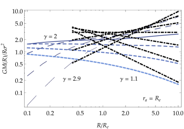
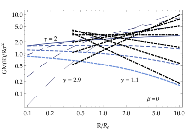
Figure 4: Aperture mass estimators where $\sigma^{2}=\sigma^{2}_{\rm ap}(R)$ (dashed lines) or $\sigma^{2}_{\rm ap}(\infty)$ (dot-dashed curves). Again, the tracer has a de Vaucouleurs luminous profile with Osipkov-Merritt anisotropy profile $\beta(r)=r^{2}/(r^{2}+r_{\rm a}^{2})$ and power-law total density $\rho_{\rm tot}\propto r^{-\gamma}$. Top panel: $r_{\rm a}=R_{\rm e};$ bottom: $r_{\rm a}\gg R_{\rm e}$. The curves are computed via eq. (2.3). The case $\gamma=2$ is marked with solid lines. The dot-dashed curves corresponding to infinite aperture sizes are the same in both panels, but are plotted twice in order to ease the comparison with the cases with finite aperture.

4.2 Aperture Masses and the Virial Limit

Measuring the velocity dispersion at the exact location $R_{\sigma}$ is not possible in practice: the observed velocity dispersion is always an average over some aperture, even when long-slit or integral-field spectroscopy is performed. On the other hand, it often happens that the radial average $\sigma^{2}_{\rm ap}({R_{\rm M}})$ is available. For example, fibre-averaged kinematics are usually measured over typical lengths that are comparable to the effective radius, as for example in the SLACS sample (Auger et al., 2010).

This suggests another class of estimators, in which $\sigma^{2}_{\rm ap}({R_{\rm M}})$ is used to measure the mass. As the dashed lines in Fig. 4 show, the sequences for $\sigma^{2}(R)/v_{\rm c}^{2}({R_{\rm M}})$ still have an appreciable ‘pinch’ at a special location ($R_{\sigma}\approx 0.5R_{\rm e}$) for a given anisotropy radius. However, there is no analogue of the intersecting regions in Fig. 3 as the anisotropy varies. The only exception is in the virial limit, which is obtained by considering the average value $\sigma^{2}_{\rm ap}(\infty)$ over the whole system. It is well-known that the virial theorem for spherical systems is independent of anisotropy. However, the aperture average over large radii is not always available with acceptable accuracy, even for nearby galaxies. A remarkable exception is given by the kinematics of resolved, extended tracers like globular clusters and planetary nebulae orbiting around the outer parts of nearby early-type galaxies (as discussed in Paper II of this series).

Figure 5: The aperture mass estimator at the radius $R_{\sigma}$ (cf Fig 4) for a de Vaucouleurs surface brightness with anisotropy profile from eq. (11), embedded in power-law total densities $\rho_{\rm tot}\propto r^{-\gamma}$. Solid curve: $\beta_{\infty}=1$ and $r_{\rm a}=R_{\rm e};$ dotted line: $\beta=0;$ dashed line: large-aperture estimator (eq. 43). The curves are computed using the formulae in Section 2.3 and Appendix B.

The dot-dashed lines in Fig. 4 show the ratio $GM(R)/[R\sigma^{2}_{\rm ap}]$ in the virial limit, which of course remains unchanged for different anisotropy profiles. Again, the luminous profile has a de Vaucouleurs form and resides in a power-law total density. For such systems, Agnello et al. (2013) have already shown for $\gamma$ within the physical interval $1<\gamma<3$

$$\mu(R)=\frac{GM(R)}{R\sigma^{2}_{\rm ap}(\infty)}=\frac{3\sqrt{\pi}\Gamma(2-\gamma/2)}{2\Gamma\left((5-\gamma)/2\right)}\times\frac{R^{2-\gamma}}{\langle R^{2-\gamma}\rangle}\ ,$$ (43)

where angled brackets represent luminosity averages. By studying the dependence of $\mu(R)$ on $\gamma$, we find that

$$\mu({R_{\rm M}})_{(\gamma=1)}=\mu({R_{\rm M}})_{(\gamma\rightarrow 3)}\ .$$ (44)

This location ${R_{\rm M}}$ can also be found analytically. In particular, if the surface brightness is of the Sérsic form given in eq (18), then

$${R_{\rm M}}=R_{\rm e}b_{n}^{-n}\sqrt{2\Gamma(3n)/\Gamma(n)}\ .$$ (45)

This implies that

$${R_{\rm M}}/R_{\rm e}\approx 1.05\mathrm{dex}[-0.019(n-4)]$$ (46)

to $0.4\%$ relative accuracy when $1<n<10$, whence ${R_{\rm M}}\approx R_{\rm e}$, as already suggested by Fig. 4.

Having determined the radius that minimizes model dependence, we must now assess the problem of systematics. The coefficient for the virial or large aperture limit takes the value ${K}=3$ in the flat rotation curve case, as shown in Fig. 5. It is somewhat smaller for a finite radius aperture. If we have no prior knowledge on the density exponent, the coefficient ${K}$ will be typically distributed uniformly in $1\lesssim{K}\lesssim 2.5$ and as $(3-{K})^{-1/2}$ when $2.5\lesssim{K}<3$. This follows from approximating the dashed curve in Fig. 5 by a parabola for ${K}\geq 2$ and straight line otherwise. The value ${K}=3$ is the most likely, because $\mu({R_{\rm M}})$ is approximately quadratic in $\gamma$ and always peaks near $\gamma=2$ (see Fig. 5 and eq. 43). However, the mean value of ${K}$ for a uniform prior on $\gamma$ is systematically lower than $3$. Its precise value depends on the photometric profile through eq. (43). For a de Vaucouleurs profile, it is straightforward to establish from Monte Carlo simulations that ${K}\approx 2.3$.

By solving the Jeans equations and fitting kinematic profiles, Wolf et al. (2010) argued that ${K}\approx 3$ and ${R_{\rm M}}=r_{1/2}\approx 1.3R_{e}$ for a diverse set of systems. However, explicit counter-examples are known for which the value ${K}=3$ is never even reached (for instance, the models of Wilkinson et al., 2002). If the results of Gavazzi et al. (2007) and Humphrey & Buote (2010) are valid in general for elliptical galaxies, then the finding that ${K}\approx 3$ means that the total density profile has $\gamma\approx 2$ in those systems near the effective radius. The same remark holds here as in the case of Cappellari et al. (2006): even if the mean behaviour is well fit by $\gamma\approx 2$ near $R_{\rm e},$ individual variations from this simple case are substantial.

If we are interested in learning about the density profile and mass content in a particular galaxy, we cannot simply rely upon ${K}\approx 3,$ as this would automatically bias our estimates towards a perfectly flat rotation curve. As a general rule, we advocate taking ${K}\approx 2.3,$ which follows from a uniform prior on $\gamma,$ and thus using the approximation

$$M({R_{\rm M}})\approx{2.3{R_{\rm M}}\over G}\sigma^{2}_{\rm ap}(\infty)$$ (47)

as a first estimate of the mass enclosed at the pinch radius in a model-independent manner. The radius ${R_{\rm M}}$ for Sérsic profiles does not vary substantially from $R_{\rm e}$. This formula (47) is valid provided $\sigma^{2}_{\rm ap}(\infty)$ is known, as this case for early-type galaxies with extended populations of globular clusters and planetary nebulae.

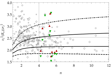
Figure 6: Ratio of squared circular velocity at the effective radius, $v_{\rm c}^{2}(R_{\rm e}),$ to the aperture-averaged velocity dispersion $\sigma^{2}_{\rm ap}(R_{\rm e})$ as a function of the Sérsic index of tracer. The solid curve corresponds to isotropy and $\gamma=2,$ the dashed line to $\gamma=2.1,\beta(R_{\rm e})=1/2$ and the dotted line to $\gamma=2.05,\beta(R_{\rm e})=1/4;$ the dot-dashed line shows the case $\gamma=2,\beta=-1/2.$ For an isotropic de Vaucouleurs tracer ($n=4$) and flat rotation curve, the ratio is approximately 5/2. Values from Peralta de Arriba et al. (2013) are shown as triangles, including (green, pointing downwards) or neglecting (red, upwards) aperture corrections. Open symbols are values from Cappellari et al. (2013), for galaxies where a Sérsic profile gives a good (circles), medium-quality (diamonds) or bad (small squares) photometric fit.

4.3 Finite Apertures

A first general feature, already noticeable from Figs 4 and 5, is that the model dependence is slightly smaller for the finite radius estimator ($\sigma^{2}=\sigma^{2}_{\rm ap}(R)$) than for the one with infinite radius. This is because in the virial limit the global average $\sigma^{2}_{\rm ap}(\infty)$ must be the same for all possible anisotropies that correspond to acceptable solutions, whence the larger variability. Second, the mass estimator at fixed $R$ and $\gamma$ generally has a lower value for the finite radius choice . This means that, if we assumed that the velocity dispersion profile is flat, we would slightly over-estimate the enclosed mass with respect to another equally plausible choice, namely isotropy ($\beta=0$) at all radii  (Agnello et al., 2013).

Obtaining pinch radii and masses from finite apertures is harder, as it is not possible to give general results unless additional conditions are imposed. A simple mass estimator can be obtained by invoking the weak homology hypothesis. For example, if we assume that $\gamma=2$ and $\beta=0,$ we readily obtain from eqs (28) and (31)

$$\sigma^{2}_{\rm ap}(R_{\rm a})=\frac{GM(R_{\rm e})}{3R_{\rm e}}\times\left(1+\frac{R_{\rm a}^{3}\int_{R_{\rm a}}^{\infty}\Sigma(s)s^{-2}\mathrm{d}s}{\int_{0}^{R_{\rm a}}\Sigma(s)s\mathrm{d}s}\right),$$ (48)

within the aperture radius $R_{\rm a}$. This formula is given by Churazov et al. (2010), who also found complementary results for completely radial ($\beta\rightarrow 1$) or tangential ($\beta\rightarrow-\infty$) orbits, still adopting $\gamma=2.$

When $\gamma\approx 2$ and $\beta$ is small, a de Vaucouleurs surface brightness leads to $\sigma^{2}_{\rm ap}(R_{\rm e})\approx 1.2\sigma^{2}_{\rm ap}(\infty).$ In this case, the enclosed mass at radii ${R_{\rm M}}\approx R_{\rm e}$ can be estimated by replacing $\sigma^{2}_{\rm ap}(\infty)$ with $\sigma^{2}_{\rm ap}(\approx R_{\rm e})$ and ${R_{\rm M}}$ with $R_{\rm e}$ in equation (47), provided the proportionality coefficient is adjusted to $\approx 3/1.2=5/2$. The mass from the finite-aperture sweetspot (Fig. 4), linearly extrapolated to the effective radius, would have a coefficient $K\approx 2.4,$ which is halfway between the large-aperture blind average and the weak homology case. The ratio $v_{c}(R_{\rm a})/\sigma_{\rm ap}(R_{\rm a})$ between circular velocity and average second moment within an aperture-radius $R_{\rm a}$ depends weakly on $R_{\rm a}/R_{\rm e},$ as long as this is around unity.

Then, a formula with ${R_{\rm M}}\approx R_{\rm a}\approx R_{\rm e}$ and $K\approx 2.4$ is the simplest to use for early-type galaxies with stellar velocity dispersion data largely confined to within one or two effective radii, when the Sérsic index is close to $n=4.$

4.4 Insights into Weak Homology

Weak homology arguments are probably appropriate for nearby early-type galaxies. Fig. 6 shows the ratio $GM(R_{\rm e})/[R_{\rm e}\sigma^{2}_{\rm ap}(R_{\rm e})]$ for Sérsic luminous components, as a function of the Sérsic index $n$ using eq. (48) and $R_{\rm a}=R_{\rm e}.$ The dynamical analysis of early-type galaxies by Cappellari et al. (2013) is summarised here by the open symbols. Regardless of the adequacy of the single Sérsic fit to the photometric profile, which is indicated by different symbols, a trend of $v_{\rm c}(R_{\rm e})/\sigma_{\rm ap}(R_{\rm e})$ with the best-fitting Sérsic index $n$ is apparent. If the mass inference is robust around $R_{\rm e},$ we can interpret this behaviour via models with different anisotropy or power-law index. In particular, galaxies with lower (higher) $n$ have stars on slightly tangential (radial) orbits on average. As shown in Krajnović et al. (2013), nearby early-type galaxies typically consist of bulge and disk components with variable size and luminosity-ratios. If the bulge (or the disk) dominates the photometric profile, that will drive the best-fitting Sérsic index towards higher (or lower) values. Then, at least part of the trend illustrated in Fig. 6 can be simply understood as a variation of bulge-to-disk ratio, with disks (bulges) having more stars on circular (radial) orbits.

Recently, Peralta de Arriba et al. (2013) have cautioned against the approximation of weak homology when compact massive galaxies, especially at higher redshift, are examined. In their analysis, they find that dynamical masses estimated as in Cappellari et al. (2006, 2013) imply negative DM fractions. Equivalently, their inferred stellar masses can exceed the dynamical estimates by almost an order of magnitude.

Since the mass within $R_{\rm e}$ is given by at least the luminous component, we can consider $GM_{\star}/[2R_{\rm e}\sigma^{2}_{\rm ap}(R_{\rm e})]$ as a lower bound on $v_{\rm c}^{2}(R_{\rm e})/\sigma^{2}_{\rm ap}(R_{\rm e})$ and check how that compares with the behaviour of nearby ellipticals. The analysis in Peralta de Arriba et al. (2013) relies on stacked spectra to obtain velocity dispersions and stellar masses, assuming a Salpeter IMF, in different redshift bins. At first sight, their results seem hard to reconcile with diverse homology arguments (Bertin et al., 2002; Cappellari et al., 2006; Taylor et al., 2010; Cappellari et al., 2013), or lensing results (Nipoti et al., 2008). However, the velocity dispersion should be averaged within the effective radius, in order to operate a fair comparison. When the simple correction $\sigma_{\rm ap}(R)\propto R^{-0.066}$ is made (c.f. Section 2.3), most of the objects fall back into the range spanned by weak homology. This is merely a consistency check, since applying the same kind of aperture correction to each galaxy tacitly assumes some kind of homology across the sample. The discrepancy is still present for the most compact ones, which may then be interpreted as a set of fast rotators. Spatially resolved kinematic information will tell if this is the case. Also, the choice of IMF may play a role. When dynamical masses are inferred via gravitational lensing, then a (universal) Salpeter IMF implies negative DM fractions for some of the SLACS galaxies (Auger et al., 2010). Interestingly, there is evidence to suggest a dichotomy in early-type galaxies. Slow rotators show a tendency towards a Salpeter IMF, and fast rotators towards a Chabrier IMF (Grillo et al., 2009; Auger et al., 2010; Emsellem et al., 2011; Suyu et al., 2012). Moreover, the IMF is known to vary with velocity dispersion (Cappellari et al., 2012; Spiniello et al., 2013). The resolution of the problem indicated by Peralta de Arriba et al. (2013) may be that both a non-universal IMF and more detailed kinematic information are required when dealing with compact massive galaxies at higher redshift, although part of the tension is already alleviated when aperture corrections are included.

5 Discussion and Conclusions

We have shown how, under the approximation of spherical symmetry, the line-of-sight velocity dispersion can be computed by means of quadratures involving the surface brightness profile $\Sigma(R)$ and a kernel that depends on the mass model and on the anisotropy. This avoids the need for explicit de-projection of the surface brightness to give the luminosity density, subsequent solution of the Jeans equations and final re-projection to give the line of sight dispersion. We have provided simple approximations for the kinematics at large distances or mild anisotropy.

The results on kinematic profiles can be adapted to include the process of averaging through circular apertures of varying size. Results for other cases (long-slit measurements, averages through an annulus, point-spread-function blurring) can be obtained by simple combinations of the ones for a circular aperture. The aperture-averaged velocity dispersion can be computed by means of single integral over the stellar density profile modulated by a kernel encoding the dependence on mass and anisotropy. If the surface brightness $\Sigma(R)$ is used, the quadratures are (at worst) double integrals and the kernels can be re-written as combinations of special functions. For some special cases (including constant anisotropy with $\beta_{\infty}=1,1/2$ and scale-free total densities), the kernel can be written explicitly in terms of elementary functions.

The aperture-averaged kinematic profiles for a de Vaucouleurs luminous component in scale-free total densities ($\rho_{\rm tot}\propto r^{-\gamma}$) reproduce the empirical behaviour observed in over 25 early-types in the SAURON survey (Cappellari et al., 2006), provided the density exponent is $\gamma=2.05\pm 0.05$ and anisotropy at the effective radius is mild ($0\leq\beta(R_{\rm e})\lesssim 0.5$). This result agrees with the findings of Koopmans et al. (2009), which are based on the analysis of 58 lensing galaxies in the SLACS sample (Bolton et al., 2006). At least as regards bulk properties, elliptical galaxies are seemingly well-represented by the simple isotropic models with a flat rotation curve.

Mass estimators can be derived by examining the kinematic profiles or aperture-averaged velocity dispersions. When the surface brightness $\Sigma(R)$ is measured with sufficient accuracy, one strategy is to determine the location ${R_{\rm M}}$ within which the enclosed mass is best constrained and the radius $R_{\sigma}$ at which kinematics should be measured in order to produce the tightest mass estimate. In the more common case of aperture-averaged kinematics, we have not found simple estimators for a de Vaucouleurs profile in scale-free total density that are truly robust against changes in anisotropy, except in the large aperture or virial limit.

For extended tracers in the outer parts of elliptical galaxies, such as globular clusters or planetary nebulae, the velocity dispersion averaged over a large aperture is in principle measurable. So, eq. (47) provides a simple estimate of the mass enclosed at a radius ${R_{\rm M}}$ that, for a de Vaucouleurs profile, is near to the effective radius. More commonly, the kinematical information is available only for populations within an effective radius or so. Then we advocate using

$$M(R_{\rm e})\approx{2.4R_{\rm e}\over G}\sigma^{2}_{\rm ap}$$ (49)

as the simplest mass-estimator in the absence of more detailed information, provided the photometric profile is bulge-dominated (that is, has a Sersic index $n\gtrsim 3.5$). This is broadly consistent with the estimator of Cappellari et al. (2006, 2013), namely that the mass enclosed near the half-light radius is $M_{1/2}\approx 2.5R_{\rm e}\sigma^{2}_{\rm ap}(R_{\rm e})/G,$ even if we have derived the result under completely different and more general hypotheses. The total mass enclosed within the effective radius appears to be a robust quantity for Sérsic-like luminous profiles, independently of the underlying mass model.

Our conclusions here are primarily theoretical. In a companion paper, we put the machinery to work in an analysis of the globular clusters of M87, and its implications for the mass distribution and orbits.

Appendix A Mathematical Details

Here, we give some of the technical details of the proofs required to derive the formula in the main body of the paper.

A.1 Proof of Equations (9) and (10)

For any function $f(x,R)$, integration by parts gives

$$\int_{R}^{y}\frac{xf(x,R)}{\sqrt{y^{2}-x^{2}}}\mathrm{d}x=f(R,R)+\int_{R}^{y}\partial_{x}\left(f(x)\right)\sqrt{y^{2}-x^{2}}\mathrm{d}x\ .$$ (50)

Assuming that $f(R,R)$ vanishes and the integrals are uniformly convergent, then we can differentiate the above with respect to $y$ to obtain eq. (9). For eq. (10), we note that:

$$\int_{R}^{\infty}\nu(r)u(r,R)\mathrm{d}r=-\frac{1}{\pi}\int_{R}^{\infty}u(r,R)\int_{r}^{\infty}\frac{\Sigma^{\prime}(y)}{\sqrt{y^{2}-r^{2}}}\mathrm{d}y\mathrm{d}r=-\frac{1}{\pi}\int_{R}^{\infty}\Sigma^{\prime}(y)\int_{R}^{y}\frac{u(r,R)}{\sqrt{y^{2}-r^{2}}}\mathrm{d}r\mathrm{d}y\ ,$$ (51)

where primes denote differentiation. Here, we again assume that $u(r,R)$ vanishes at $r=R$ and all the integrals are well defined, Integrating by parts in $y$ and using eq. (9) with $f(r)=u(r,R)/r$, then eq. (10) follows if we set $u(r,R)=M(r)\left[\sqrt{r^{2}-R^{2}}+k_{\beta}(R,r)\right]/r^{2}.$

A.2 Proof of Equations (15) and (17)

Let us define $F(r)=GM(r)/r^{2}$ for conciseness. We start directly from eq. (4), multiply by $2\pi R,$ integrate in $0<R<R_{\rm a}$ and reverse orders of integration between $R$ and $r:$

$$L(R_{\rm a})\sigma^{2}_{\rm ap}(R_{\rm a}) = 4\pi\int_{0}^{R_{\rm a}}R\int_{R}^{\infty}\left(1-\beta(r)\frac{R^{2}}{r^{2}}\right)\frac{r}{\sqrt{r^{2}-R^{2}}}\int_{r}^{\infty}F(s)J_{\beta}(r,s)\mathrm{d}s\mathrm{d}r\mathrm{d}R$$

$$= 4\pi\int_{0}^{R_{\rm a}}\left[\int_{0}^{r}R\left(1-\beta(r)\frac{R^{2}}{r^{2}}\right)\frac{r}{\sqrt{r^{2}-R^{2}}}\mathrm{d}R\right]\int_{r}^{\infty}F(s)J_{\beta}(r,s)\mathrm{d}s\mathrm{d}r$$

$$+ 4\pi\int_{R_{\rm a}}^{\infty}\left[\int_{0}^{R_{\rm a}}R\left(1-\beta(r)\frac{R^{2}}{r^{2}}\right)\frac{r}{\sqrt{r^{2}-R^{2}}}\mathrm{d}R\right]\int_{r}^{\infty}F(s)J_{\beta}(r,s)\mathrm{d}s\mathrm{d}r\ .$$

The integrals in $R$ are easily performed and lead to

$$L(R_{\rm a})\sigma^{2}_{\rm ap}(R_{\rm a}) = 4\pi\int_{0}^{\infty}r^{2}(1-\frac{2}{3}\beta(r))\int_{r}^{\infty}F(s)J_{\beta}(r,s)\mathrm{d}s\mathrm{d}r$$

$$- 4\pi\int_{R_{\rm a}}^{\infty}\left(r\sqrt{r^{2}-R_{\rm a}^{2}}-\frac{2}{3}\beta(r)\frac{(r^{2}-R_{\rm a}^{2})^{3/2}}{r}\right)\int_{r}^{\infty}F(s)J_{\beta}(r,s)\mathrm{d}s\mathrm{d}r$$

$$+ 4\pi R_{\rm a}^{2}\int_{R_{\rm a}}^{\infty}\frac{\beta(r)}{r}\sqrt{r^{2}-R_{\rm a}^{2}}\int_{r}^{\infty}F(s)J_{\beta}(r,s)\mathrm{d}s\mathrm{d}r\ .$$

The last line gives the third term in eq. (15), provided we exchange orders of integration between $r$ and $s.$ For the other two terms, we also observe that $\partial_{r}J_{\beta}(r,s)=-2\beta(r)J_{\beta}(r,s)/r$ and $J(s,s)=J(r,r)=1,$ so that

$$\int_{0}^{s}r^{2}J_{\beta}(r,s)\mathrm{d}r = \frac{1}{3}s^{3}+\frac{2}{3}\int_{0}^{s}\beta(r)r^{2}J_{\beta}(r,s)\mathrm{d}r\ ,$$ (54)

$$\int_{R_{\rm a}}^{s}r\sqrt{r^{2}-R_{\rm a}^{2}}J_{\beta}(r,s)\mathrm{d}r = \frac{1}{3}(s^{2}-R_{\rm a}^{2})^{3/2}+\frac{2}{3}\int_{R_{\rm a}}^{s}\beta(r)J_{\beta}(r,s)\frac{(r^{2}-R^{2}_{\rm a})^{3/2}}{r}\mathrm{d}r\ ,$$ (55)

whence eq. (15), whose first line is obtained via $\partial_{r}M(r)=4\pi\rho_{\rm tot}(r)r^{2}.$ Eq. (17) follows by Abel deprojection of $\nu$ and the same line of reasoning that led to eq. (10).

A.3 Proof of Equations (20) and (24)

When $\beta$ or $(s-r)/r$ are small, we may Taylor expand eq. (3) to obtain

$$J_{\beta}(r,s)\ \sim\ 1+2\int_{r}^{s}\beta(u)\mathrm{d}u/u.$$ (56)

Then, we can approximate $J_{\beta}\sim 1$ in the integrals $k_{\beta}(R,x)$ and $Z_{\beta}(R,x),$ to obtain first order approximations in $|\beta|$ and $x-R.$ For higher order terms, the whole behaviour of $\beta$ is necessary. Eq. (20) is valid in general, whereas eq. (24) is obtained in the limit $R\gg r_{\rm a},$ i.e. $\beta\sim\beta_{\infty}.$ An expansion accounting for other terms in $r_{\rm a}/R$ is

$$k_{\beta}(R,x)\ \sim\ -\beta(R)(x^{2}-R^{2})^{1/2}+\beta_{\infty}\frac{(1-\tfrac{2}{3}(\beta_{\infty}-r_{\rm a}^{2}/R^{2}))}{(1+r_{\rm a}^{2}/R^{2})^{2}}(x^{2}/R^{2}-1)^{3/2}R+\mathcal{O}(\beta_{\infty}(x^{2}/R^{2}-1)^{5/2})R\ .$$ (57)

When $\Sigma$ decays sufficiently fast, higher-order terms are suppressed and we obtain the asymptotic expressions

$$k_{\beta}(R,x)\sim-\beta(R)(x^{2}-R^{2})^{1/2}\ ,$$ (58)

$$Z_{\beta}(R,y)\sim\frac{1}{3R^{2}}(y^{2}-R^{2})^{3/2}.$$ (59)

These are usually sufficient to approximate $\sigma_{p}$ and $\sigma_{\rm ap}.$ The main exception is the case $\beta\rightarrow 1,$ when the first non-trivial term in $\sqrt{x^{2}-R^{2}}+k_{\beta}(R,x)$ is proportional to $(x^{2}-R^{2})^{3/2}.$

A.4 Proof of Equations (21), (25) and (28)

We start by noting that

$$\partial_{r}\left(r^{-\gamma}(r^{2}-R^{2})^{j/2}\right)\ =\ r^{-\gamma-1}(r^{2}-R^{2})^{j/2-1}\left[(j-\gamma)r^{2}+\gamma R^{2}\right]\ .$$ (60)

If $\rho_{\rm tot}=\rho_{0}(r/r_{0})^{-\gamma},$ then from eq. (10):

$$\Sigma\sigma^{2}_{p}(R)=\frac{8G\rho_{0}r_{0}^{\gamma}}{3-\gamma}\int_{R}^{\infty}y\Sigma(y)\int_{R}^{y}\frac{\partial_{r}\left(r^{-\gamma}(\sqrt{r^{2}-R^{2}}+k_{\beta}(R,r)\right)}{\sqrt{y^{2}-r^{2}}}\mathrm{d}r\mathrm{d}y\ .$$ (61)

Now, eq. (21) (resp. 25) follows by exploiting equation (60) and eq. (20) (resp. 24), via the replacements $R=xy$ and $r=\sqrt{t}y.$

An analogous argument can be followed to obtain the average velocity dispersion within a circular aperture. However, an alternative procedure leads to more convenient formulae such as eqs. (28) and (29). We start by recasting eq. (17) as

$$\sigma^{2}_{\rm ap}(R)\ =\ \frac{4G}{3L(R)}\left[I(0)-I(R)\right]\ ,$$ (62)

where

$$I(R)\ \equiv\ \int_{R}^{\infty}\Sigma(s)s\int_{R}^{s}\frac{\partial_{r}\left(M(r)(r^{2}-R^{2})^{3/2}/r^{3}\right)}{\sqrt{s^{2}-r^{2}}}\mathrm{d}r\mathrm{d}s\ =\ \int_{R}^{\infty}\Sigma(s)\frac{\mathrm{d}}{\mathrm{d}s}\int_{R}^{s}\frac{M(r)(r^{2}-R^{2})^{3/2}/r^{2}}{\sqrt{s^{2}-r^{2}}}\mathrm{d}r\mathrm{d}s\ .$$

For a power-law total density $\rho_{\rm tot}(r)=\rho_{0}(r/r_{0})^{-\gamma},$ we have

$$I(R)\ =\ \frac{4\pi\rho_{0}r_{0}^{\gamma}}{3-\gamma}\int_{R}^{\infty}\Sigma(R)\frac{\mathrm{d}}{\mathrm{d}s}\int_{R}^{s}\frac{r^{1-\gamma}(r^{2}-R^{2})^{3/2}}{\sqrt{s^{2}-r^{2}}}\mathrm{d}r\mathrm{d}s\ .$$ (63)

The derivative with respect to $s$ is:

$$\frac{\mathrm{d}}{\mathrm{d}s}\int_{R}^{s}\frac{r^{1-\gamma}(r^{2}-R^{2})^{3/2}}{\sqrt{s^{2}-r^{2}}}\mathrm{d}r = \frac{\mathrm{d}}{\mathrm{d}s}\left(s^{4-\gamma}\int_{R/s}^{1}\frac{u^{1-\gamma}(u^{2}-(R/s)^{2})^{3/2}}{\sqrt{1-u^{2}}}\mathrm{d}u\right)$$ (64)

$$= (4-\gamma)s^{3-\gamma}\int_{R/s}^{1}\frac{u^{1-\gamma}(u^{2}-(R/s)^{2})^{3/2}}{\sqrt{1-u^{2}}}\mathrm{d}u+3s^{3-\gamma}\left(\frac{R}{s}\right)^{2}\int_{R/s}^{1}\frac{u^{1-\gamma}\sqrt{u^{2}-(R/s)^{2}}}{\sqrt{1-u^{2}}}\mathrm{d}u\ .$$

Eq. (28) then follows by using $(u^{2}-(R/s)^{2})^{3/2}=(u^{2}-(R/s)^{2})\sqrt{u^{2}-(R/s)^{2}},$ splitting the first integral in equation (64) and summing the two terms proportional to $(R/s)^{2}.$

Appendix B Special Cases

B.1 Anisotropy Profiles with Analytic Kernels

Here, we list some special cases of the kernels $k_{\beta}(R,x)$ defined in eq. (8) and $Z_{\beta}(R,y)$ defined in eq. (2.3) We recollect that these kernels are needed in the quadratures for the line of sight and aperture-averaged velocity dispersions respectively.

For the anisotropy profile (11), the kernel $k_{\beta}$ can be expressed in terms of hypergeometric functions, as indicated in eq. (19). The corresponding result for $Z_{\beta}$ was not given in the main text, and so we report it here

$$Z_{\beta}(R,y)=\frac{\beta_{\infty}}{(4\beta_{\infty}^{2}-1)\sqrt{y^{2}-R^{2}}}\left[(r_{\rm a}^{2}+R^{2})_{2}F_{1}\left(1,-\beta_{\infty}\!-\!\frac{1}{2},\frac{1}{2},z\right)\!-\!(y^{2}\!+\!r_{\rm a}^{2})\!-2\!\beta_{\infty}(y^{2}\!-\!R^{2})\right]\ ,$$ (65)

where we have put $z=(R^{2}-y^{2})/(r_{\rm a}^{2}+R^{2})$. The kernel is regular at $\beta_{\infty}=\tfrac{1}{2}$ and $y=R$, as may be confirmed by careful Taylor expansion.

Some special cases reduce to elementary functions, and we briefly note these results here. In the Osipkov-Merritt case $\beta_{\infty}=1$, we have

$$k_{\beta}(R,x) = \frac{1}{2(r_{\rm a}^{2}+R^{2})^{3/2}}\left[(2r_{\rm a}^{2}+R^{2})(r_{\rm a}^{2}+x^{2})\mathrm{arctan}\sqrt{\frac{x^{2}-R^{2}}{r_{\rm a}^{2}+R^{2}}}-(2r_{\rm a}^{2}+3R^{2})\sqrt{(x^{2}-R^{2})(r_{\rm a}^{2}+R^{2})}\right],$$ (66)

$$Z_{\beta}(R,y) = \frac{1}{2\sqrt{r_{\rm a}^{2}+R^{2}}}\left[(r_{\rm a}^{2}+y^{2})\mathrm{arcsin}\sqrt{\frac{y^{2}-R^{2}}{y^{2}+r_{\rm a}^{2}}}-\sqrt{(y^{2}-R^{2})(R^{2}+r_{\rm a}^{2})}\right]\ .$$ (67)

When $\beta_{\infty}=\tfrac{1}{2}$, we have

$$k_{\beta}(R,x) = \frac{\sqrt{r_{\rm a}^{2}+x^{2}}}{2(r_{\rm a}^{2}+R^{2})}\left[2(r_{\rm a}^{2}+R^{2})\mathrm{arcsinh}\sqrt{\frac{x^{2}-R^{2}}{R^{2}+r_{\rm a}^{2}}}-(2r_{\rm a}^{2}+3R^{2})\sqrt{\frac{x^{2}-R^{2}}{r_{\rm a}^{2}+x^{2}}}\right],$$ (68)

$$Z_{\beta}(R,y) = \frac{\sqrt{r_{\rm a}^{2}+y^{2}}}{2}\left(\mathrm{arcsinh}\sqrt{\frac{y^{2}-R^{2}}{r_{\rm a}^{2}+R^{2}}}-\sqrt{\frac{y^{2}-R^{2}}{r_{\rm a}^{2}+y^{2}}}\right).$$ (69)

When $r_{\rm a}=0$, the models have constant anisotropy $\beta_{\infty}$ and we obtain

$$k_{\beta}(R,x) = \beta_{\infty}R(x/R)^{2\beta_{\infty}}\left[B\left(\beta_{\infty}-\frac{1}{2},\frac{1}{2}\right)-B\left(\frac{R^{2}}{x^{2}},\beta_{\infty}-\frac{1}{2},\frac{1}{2}\right)+\frac{3}{2}B\left(\frac{R^{2}}{x^{2}},\beta_{\infty}+\frac{1}{2},\frac{1}{2}\right)-\frac{3}{2}B\left(\beta_{\infty}+\frac{1}{2},\frac{1}{2}\right)\right],$$ (70)

$$Z_{\beta}(R,y) = \frac{\beta_{\infty}}{2}R(y/R)^{2\beta_{\infty}}\left[B\left(\frac{3}{2},\beta_{\infty}-\frac{1}{2}\right)-B\left(\frac{R^{2}}{y^{2}},\beta_{\infty}-\frac{1}{2},\frac{3}{2}\right)\right],$$ (71)

where $B(z,a,b)$ is the incomplete Beta function and $B(a,b)=B(0,a,b)$. We note that equivalent formulae for the kernel $k_{\beta}$ in the Osipkov-Merrit and constant anisotropy cases have previously been given by Mamon & Łokas (2005b).

B.2 Large Radii and Small Anisotropies

At large radii and/or small anisotropies, the line of sight velocity dispersion can be written more conveniently:

$$\frac{\Sigma(R)\sigma^{2}_{\rm p}(R)}{1-\beta(R)} \sim 8G\int_{R}^{\infty}\Sigma(y)y\int_{R}^{y}\rho_{\rm tot}(x)\frac{\sqrt{x^{2}-R^{2}}}{x^{3}\sqrt{y^{2}-x^{2}}}\mathrm{d}x\mathrm{d}y+8GR^{-3}\left(\int_{0}^{R}\rho_{\rm tot}(x)x^{2}\mathrm{d}x\right)\int_{R}^{\infty}\Sigma(y)yA(1,y/R)\mathrm{d}y$$ (72)

$$+ 8GR^{-3}\int_{R}^{\infty}\Sigma(y)y\int_{R}^{y}\rho_{\rm tot}(x)x^{2}A(x/R,y/R)\mathrm{d}x\mathrm{d}y\ ,$$

where the integral

$$A(\chi,\xi)=\int_{\chi}^{\xi}\frac{3-2r^{2}}{\sqrt{(\xi^{2}-r^{2})(r^{2}-\chi^{2})}}\frac{\mathrm{d}r}{r^{4}}$$ (73)

does not depend on any mass model and can be tabulated separately.

Similarly, for aperture-averaged dispersions, when anisotropy is sufficiently small, we have

$$\frac{3L(R)\sigma^{2}_{\rm ap}(R)}{16\pi G} \sim \int_{0}^{\infty}\Sigma(y)y\int_{0}^{y}\frac{\rho_{\rm tot}(x)x^{2}\mathrm{d}x}{\sqrt{y^{2}-x^{2}}}-3(1-\beta(R))R^{-1}\left(\int_{0}^{R}\rho_{\rm tot}(x)x^{2}\mathrm{d}x\right)\int_{R}^{\infty}\Sigma(y)yB(1,y/R)\mathrm{d}y$$ (74)

$$- 3(1-\beta(R))R^{-1}\int_{R}^{\infty}\Sigma(y)y\int_{R}^{y}\rho_{\rm tot}(x)x^{2}B(x/R,y/R)\mathrm{d}x\mathrm{d}y\ ,$$

where again

$$B(\chi,\xi)=\int_{\chi}^{\xi}\sqrt{\frac{r^{2}-\chi^{2}}{\xi^{2}-r^{2}}}\frac{\mathrm{d}r}{r^{4}}\ .$$ (75)

is independent of any model adopted and can be tabulated separately.

References

- Abadi et al. (2010) Abadi, M. G., Navarro, J. F., Fardal, M., Babul, A., & Steinmetz, M. 2010, MNRAS, 407, 435
- Agnello & Evans (2012a) Agnello, A., & Evans, N. W. 2012a, ApJL, 754, L39
- Agnello & Evans (2012b) Agnello, A., & Evans, N. W. 2012b, MNRAS, 422, 1767
- Agnello et al. (2013) Agnello, A., Auger, M. W., & Evans, N. W. 2013, MNRAS, 429, L35
- Amorisco & Evans (2011) Amorisco, N. C., & Evans, N. W., 2011, MNRAS, 411, 2118
- An & Evans (2011) An, J. H., & Evans, N. W. 2011, MNRAS, 413, 1744
- Auger et al. (2010) Auger, M. W., Treu, T., Bolton, A. S., et al. 2010, ApJ, 724, 511
- Bacon et al. (2001) Bacon, R., Copin, Y., Monnet, G., et al. 2001, MNRAS, 326, 23
- Bertin et al. (1994) Bertin, G., Bertola, F., Buson, L. M., et al. 1994, AA, 292, 381
- Bertin et al. (2002) Bertin, G., Ciotti, L., & Del Principe, M. 2002, AA, 386, 149
- Binney & Mamon (1982) Binney, J., & Mamon, G. A., 1982, MNRAS, 200, 361
- Blumenthal et al. (1986) Blumenthal, G. R., Faber, S. M., Flores, R.,& Primack, J. R. 1986, ApJ, 301, 27
- Bolton et al. (2006) Bolton, A. S., Burles, S., Koopmans, L. V. E., Treu, T., & Moustakas, L. A. 2006, ApJ, 638, 703
- Cappellari et al. (2006) Cappellari, M., Bacon, R., Bureau, M., et al. 2006, MNRAS, 366, 1126
- Cappellari (2008) Cappellari, M. 2008, MNRAS, 390, 71
- Cappellari et al. (2012) Cappellari, M., McDermid, R. M., Alatalo, K., et al. 2012, Nat, 484, 485
- Cappellari et al. (2013) Cappellari, M., Scott, N., Alatalo, K., et al. 2013, MNRAS, 432, 1709
- Carollo et al. (1995) Carollo, C. M., de Zeeuw, P. T., van der Marel, R. P. Danziger, I. J., & Qian, E. E. 1995, ApJL, 441, L25
- Cattaneo et al. (2011) Cattaneo, A., Mamon, G. A., Warnick, K., & Knebe, A. 2011, AA, 533, A5
- Churazov et al. (2010) Churazov, E., Tremaine, S., Forman, W., et al. 2010, MNRAS, 404, 1165
- Ciotti & Bertin (1999) Ciotti, L., & Bertin, G. 1999, AA, 352, 447
- Ciotti et al. (2009) Ciotti, L., Morganti, L., & de Zeeuw, P. T. 2009, MNRAS, 393, 491
- Courteau et al. (2013) Courteau, S., Cappellari, M., de Jong, R. S., et al. 2013, arXiv:1309.3276
- de Vaucouleurs (1948) de Vaucouleurs, G. 1948, Annales d’Astrophysique, 11, 247
- Dekel et al. (2005) Dekel, A., Stoehr, F., Mamon, G. A., et al. 2005, Nat, 437, 707
- Di Cintio et al. (2013) Di Cintio, A., Brook, C. B., Macciò, A. V., et al. 2013, MNRAS, 2583
- Dubois et al. (2013) Dubois, Y., Gavazzi, R., Peirani, S., & Silk, J. 2013, MNRAS, 433, 3297
- Emsellem et al. (1994) Emsellem, E., Monnet, G., & Bacon, R. 1994, AA, 285, 723
- Emsellem et al. (2011) Emsellem, E., Cappellari, M., Krajnović, D., et al. 2011, MNRAS, 414, 888
- Evans (1994) Evans, N. W. 1994, MNRAS, 267, 333
- Evans & de Zeeuw (1994) Evans, N. W., & de Zeeuw, P. T. 1994, MNRAS, 271, 202
- Falco et al. (2013) Falco, M., Mamon, G. A., Wojtak, R., Hansen, S. H., & Gottlöber, S. 2013, MNRAS, 436, 2639
- Gavazzi et al. (2007) Gavazzi, R., Treu, T., Rhodes, J. D., et al. 2007, ApJ, 667, 176
- Gerhard et al. (1998) Gerhard, O., Jeske, G., Saglia, R. P., & Bender, R. 1998, MNRAS, 295, 197
- Gerhard et al. (2001) Gerhard, O., Kronawitter, A., Saglia, R. P., & Bender, R. 2001, AJ, 121, 1936
- Grillo et al. (2009) Grillo, C., Gobat, R., Lombardi, M., & Rosati, P. 2009, AA, 501, 461
- Hilz et al. (2013) Hilz, M., Naab, T.,& Ostriker, J. P. 2013, MNRAS, 429, 2924
- Humphrey & Buote (2010) Humphrey, P. J., & Buote, D. A. 2010, MNRAS, 403, 2143
- Illingworth (1976) Illingworth, G. 1976, ApJ, 204, 73
- Johansson et al. (2012) Johansson, P. H., Naab, T., & Ostriker, J. P. 2012, ApJ, 754, 115
- Krajnović et al. (2005) Krajnović, Cappellari, M., Emsellem, E., McDermid, R. M., & de Zeeuw, P. T. 2005, MNRAS, 357, 1113
- Koopmans (2006) Koopmans, L. V. E. 2006, EAS Publications Series, 20, 161
- Koopmans et al. (2009) Koopmans, L. V. E., Bolton, A., Treu, T., et al. 2009, ApJL, 703, L51
- Krajnović et al. (2013) Krajnović, D., Alatalo, K., Blitz, L., et al. 2013, MNRAS, 432, 1768
- Lackner & Ostriker (2010) Lackner, C. N., & Ostriker, J. P. 2010, ApJ, 712, 88
- Lanzoni & Ciotti (2003) Lanzoni, B., & Ciotti, L. 2003, AA, 404, 819
- Laporte et al. (2013) Laporte, C. F. P., Walker, M. G., & Peñarrubia, J. 2013, MNRAS, 433, L54
- Lima Neto et al. (1999) Lima Neto, G. B., Gerbal, D., & Márquez, I. 1999, MNRAS, 309, 481
- Mamon & Łokas (2005a) Mamon, G. A., & Łokas, E. L. 2005a, MNRAS, 362, 95; Erratum in MRAS 370, 1581 (2006)
- Mamon & Łokas (2005b) Mamon, G. A., & Łokas, E. L. 2005b, MNRAS, 363, 705
- Mamon & Boué (2010) Mamon, G. A., & Boué, G. 2010, MNRAS, 401,2433
- Mamon et al. (2013) Mamon, G. A., Biviano, A., & Boué, G. 2013, MNRAS, 429, 3079
- Merritt (1985) Merritt D., 1985, AJ, 90, 1027
- Merritt & Saha (1993) Merritt, D., & Saha, P. 1993, ApJ, 409, 75
- Navarro et al. (1996) Navarro, J. F., Frenk, C. S., & White, S. D. M. 1996, ApJ, 462, 563
- Nipoti et al. (2008) Nipoti, C., Treu, T., & Bolton, A. S. 2008, MNRAS, 390, 349
- Nipoti et al. (2012) Nipoti, C., Treu, T., Leauthaud, A., et al. 2012, MNRAS, 422, 1714
- Osipkov (1979) Osipkov L. P., 1979, Pis’ma Astr. Zh., 5, 77
- Peralta de Arriba et al. (2013) Peralta de Arriba, L., Balcells, M., Falcón-Barroso, J., & Trujillo, I. 2013, arXiv:1307.4376
- Power et al. (2011) Power, C., Zubovas, K., Nayakshin, S., & King, A. R. 2011, MNRAS, 413, L110
- Prugniel & Simien (1997) Prugniel, P., & Simien, F. 1997, AA, 321, 111
- Remus et al. (2013) Remus, R.-S., Burkert, A., Dolag, K., et al. 2013, ApJ, 766, 71
- Richstone & Tremaine (1984) Richstone, D. O., & Tremaine, S. 1984, ApJ, 286, 27
- Schwarzschild (1979) Schwarzschild, M. 1979, ApJ, 232, 236
- Sersic (1968) Sersic, J. L. 1968, Cordoba, Argentina: Observatorio Astronomico, 1968,
- Spiniello et al. (2013) Spiniello, C., Trager, S., Koopmans, L. V. E., & Conroy, C. 2013, arXiv:1305.2873
- Suyu et al. (2012) Suyu, S. H., Hensel, S. W., McKean, J. P., et al. 2012, ApJ, 750, 10
- Treu & Koopmans (2004) Treu, T., & Koopmans, L. V. E. 2004, ApJ, 611, 739
- Taylor et al. (2010) Taylor, E. N., Franx, M., Brinchmann, J., van der Wel, A., & van Dokkum, P. G. 2010, ApJ, 722, 1
- van der Marel (1994) van der Marel, R. P. 1994, MNRAS, 270, 271
- Walker et al. (2009) Walker, M. G., Mateo, M., Olszewski, E. W., et al. 2009, ApJ, 704, 1274
- Walker & Peñarrubia (2011) Walker, M. G., & Peñarrubia, J. 2011, ApJ, 742, 20
- Wilkinson et al. (2002) Wilkinson, M. I., Kleyna, J., Evans, N. W., & Gilmore, G. 2002, MNRAS, 330, 778
- Wolf et al. (2010) Wolf, J., Martinez, G. D., Bullock, J. S., et al. 2010, MNRAS, 406, 1220