The solar chromosphere observed at 1 Hz and $0\farcs 2$ resolution

Abstract

We recently reported extremely rapid changes in chromospheric fine structure observed using the IBIS instrument in the red wing of H$\alpha$. Here, we examine data obtained during the same observing run (August 7 2010), of a mature active region NOAA 11094. We analyze more IBIS data including wavelength scans and data from the Solar Dynamics Observatory, all from within a 30 minute interval. Using a slab radiative transfer model, we investigate the physical nature of fibrils in terms of tube-like vs. sheet-like structures. Principal Component Analysis shows that the very rapid H$\alpha$ variations in the line wings depend mostly on changes of line width and line shift, but for Ca II 854.2 the variations are dominated by changes in column densities. The tube model must be rejected for a small but significant class of fibrils undergoing very rapid changes. If our wing data arise from the same structures leading to “type II spicules”, our analysis calls into question much recent work. Instead the data do not reject the hypothesis that some fibrils are optical superpositions of plasma collected into sheets. We review how Parker’s theory of tangential discontinuities naturally leads to plasma collecting into sheets, and show that the sheet picture is falsifiable. Chromospheric fine structures seem to be populated by both tubes and sheets. We assess the merits of spectral imaging versus slit spectroscopy for future studies.

1 Introduction

We have previously questioned the traditional interpretation that chromospheric fine structure, as revealed by H$\alpha$ data for example, corresponds to plasma that fills narrow tubes of magnetic flux (Judge et al., 2011, 2012, henceforth JTL11, JRC12). In JRC12 we argued that at least some newly observed properties of the fine structure are inconsistent with the traditional picture, and instead have proposed that the fine structure contains at least some sheet-like structures, corresponding perhaps to the magnetic tangential discontinuities (TDs) whose existence has been argued on theoretical grounds by Parker (1994). The primary observational evidence we cite is the rapid appearance and disappearance of “typical” fine structures simultaneously along their entire length of 3–5,000 km, seen in absorption at one particular wavelength in the H$\alpha$ line. By “rapid” we mean super-Alfvénic apparent speeds, so that no propagating disturbance can account for the rapid appearance of a feature all along its length. The observed behavior led us to discount oblique wave propagation and standing waves, the latter on the grounds that the features appear suddenly out of nowhere, whereas standing waves require special boundary conditions and finite times to become established. This point stands in contrast to the claims of others, and it is addressed here in our Appendix A.

In the light of the recent launch of the IRIS spacecraft, and to shed further light on the problem, here we re-analyze data reported earlier (JRC12) with additional data. We try to refute two competing hypotheses: (1) that fine structure corresponds to plasma constrained to flow along and within narrow tubes or “straws” of magnetic flux, and (2) that fine structure corresponds to material trapped within surfaces of tangential discontinuity embedded in an otherwise continuous structure. The answers are not just of academic interest, important physical consequences include the following: the interpretation of apparent motions in terms of real motion vs. phase effects; the existence of magnetic TDs in plasmas in a low $\beta$ state ($\beta$ is the ratio of plasma to magnetic pressure); the long standing problem of energy transport in the lower transition region.

We regard both hypotheses as worthy of study. Indeed, the evidence in support of tubes is strong in photospheric features such as sunspot penumbrae, and in certain kinds of chromospheric phenomena called “dynamic fibrils” (Hansteen et al., 2006), later associated with the “spicule of type I” documented by de Pontieu et al. (2007). But we believe that the question remains more open for the very different spicules of type II that are believed to carry mass, momentum and energy into the corona (see, e.g., Zhang et al., 2012), despite claims that the evidence only supports the traditional, flux tube picture (e.g. Sekse et al., 2013a). Several studies based upon further theoretical and observational considerations have been published questioning the role of type II spicules in coronal physics (Klimchuk, 2012; Tripathi and Klimchuk, 2013; Patsourakos et al., 2013).

Below we refer to all dark “chromospheric fine structures” which appear on the solar disk like thin, straw-like structures, simply as “fibrils”.

2 Observations

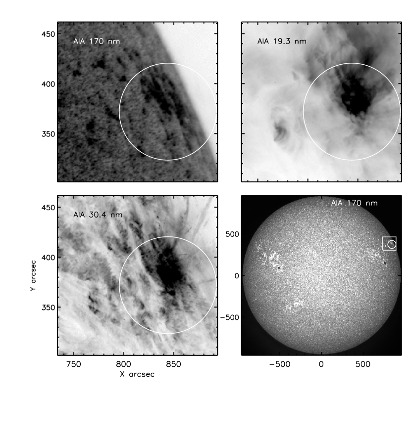
Figure 1: The field of view of the IBIS observations is shown as a circle against images obtained between 14:25:19 and 14:25:31 UT on 7th August 2010, from the AIA instrument on the SDO spacecraft. The image densities are reversed and are proportional to the square root of the brightness, except for the bottom right image.

Spectroscopic observations of a limb region, covering a 97″ diameter circular field, were obtained on 7th August 2010 using the IBIS instrument (Cavallini, 2006) with the Dunn Solar Telescope at Sunspot, NM. The field of view centered near the NW solar limb between 14:10 and 14:35 UT. Co-alignment of the time average of images obtained in the red wing of H$\alpha$ with plages and sunspots in an image at 170 nm obtained at 14:25 UT from SDO AIA yields a target center of $x=844\arcsec$, $y=372\arcsec$, with an uncertainty of an arc second. Images of the low chromosphere, transition region and corona from the AIA instrument (Lemen et al., 2012) on the Solar Dynamics Observatory (SDO) spacecraft includes the field of view of the IBIS observations in Figure 1. The field of view observed includes a mature active region (NOAA 11261) with a small sunspot which was used as the lock point for the adaptive optics system. This region produced many C- and several M- class flares during the preceding disk passage, but flaring had stopped two days before our observations were made.

Time averages of red and blue wing IBIS images are shown in Figure 2. The circled areas highlight regions with significant numbers of narrow, long fibrils; they are seen in this average plot as “smudges” as they come and go during the averaging. The scans run with IBIS are summarized in Figure 3. Each point in the plot represents one fully processed image (see below) at a given wavelength. There are several time series shown (many closely packed abscissa points at one ordinate position), as well as some full wavelength scans between 14:28 and 14:31 UT. The longest time series, marked “JRC2012”, was analyzed by JRC12.

The raw IBIS data consist of counts as a function of position on the sky, the region observed being shown in Figure 2. Each exposure is of 60 msec integration time except for two H$\alpha$ bursts at 14:31:32 and 14:32:46 (500 frames each) which had 25 msec exposures. The camera accumulated data at a 0.1s cadence. The data were processed to include standard dark, flat and linearization corrections. The time series data – all those data shown in Figure 3 except the wavelength scans obtained between 14:28 and 14:31 UT – were further processed using speckle interferometric (Wöger et al., 2008) and multi-frame blind deconvolution (MFBD) techniques (Löfdahl, 2002), to correct residual seeing-induced errors. The cadence of the seeing-corrected time series datasets is 1 sec (MFBD) and 5 sec (speckle). In the time-series reconstructions center-to-limb brightness variations are removed. The wavelength scans also included corrections for the slightly variable wavelengths across the field of view that results from the “classical mount” of the IBIS etalons. Such corrections, relying on interpolations in wavelength, cannot be applied to the fixed-wavelength, time series data, but its effects are irrelevant to our results as we deal mostly with relative variations at any given spatial position.

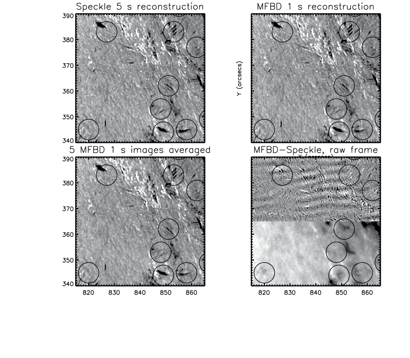
Figure 4: A comparison of images processed using the MFBD and speckle techniques at H$\alpha$ +0.11 nm. The three complete images show data with a linear color table between 1% and 99% of the brightness distributions The lower right image shows the difference between the two 5s images (upper half) scaled between 0.8 and 1.2 of the median brightness, and an unprocessed image from the wavelength scan series for comparison, again scaled between 1% and 99%. The center-to-limb variation is visible in the unprocessed data.

The MFBD and speckle image reconstructions are not identical, as expected. Figure 4 compares MFBD and speckle images taken at $+0.11$nm from line center, over a small region of the FOV. We built the MFBD dataset from ten consecutive 0.1s frames, but the speckle dataset was built from fifty frames. In the Figure we juxtapose two sets of speckle and MFBD images taken in H$\alpha$. These reconstructions are built from the same raw frames, highlighting the differences between the two techniques, as well as differences between data recovered at 1 and 5 second cadences. While there is an observable difference between MFBD and speckle images in terms of definition of structures, fringe-like artifacts and brightness/depth levels, the differences are small compared with the robust properties of the obvious fibril-like features analyzed here.

The figure also shows (lower right panel, bottom half of the image) an unprocessed image from the wavelength scan series. The unprocessed image is of much lower resolution, showing the power of reconstructions. This difference must be kept in mind when comparing reconstructed data with the wavelength scan data below (section 3.2). Clearly, post-processing as well as adaptive optics are important for the measurement of such fine structures as fibrils.

3 Analysis

3.1 A simple model

We adopt a simple model for the formation of the fibril intensities. We consider the fibril absorption to occur in a slab of plasma which has associated with it microscopic (thermal and turbulent) velocities, and macroscopic line-of-sight (flow) velocities. These quantities translate to a local Doppler line width $w$ and shift $s$ respectively. Our goal is to relate changes in the line intensity at a given frequency to changes in the minimum number of parameters required: these are the line optical depth, the line shift, and the line width. Assuming the source function in the slab is small compared with the photospheric intensity $I^{0}_{x}$, and slab optical depths $\delta\tau_{x}$ are $\ll 1$, the change in intensity at a (normalized) frequency $x$ through the slab, is (e.g. JRC12)

$$\delta I_{x}=-I^{0}_{x}\delta\tau_{x}\,=-I^{0}_{x}\,a_{ij}\,\times$$ (1)

$$\left(\phi_{x}\delta(n_{i}\Delta)+(n_{i}\Delta)\left\{\left(\frac{\partial\phi_{x}}{\partial s}\right)_{w}{\delta s}+\left(\frac{\partial\phi_{x}}{\partial w}\right)_{s}{\delta w}\right\}\right).$$

Here $a_{ij}$ is the absorption cross section for radiative transitions between atomic levels $i$ and $j$ ($a_{ij}=\frac{\pi e^{2}}{mc}f_{ij}$ with $f_{ij}$ the absorption oscillator strength); $I^{0}_{x}$ the incident photospheric intensity; $\phi_{x}$ the normalized absorption profile ($\int_{-\infty}^{\infty}\phi_{x}dx=1$); $n_{i}\Delta$ is the population density of the lower level of the line transition times the geometrical thickness $\Delta$ of the absorbing slab. In this model changes in $(n_{i}\Delta)$, $s$ and $w$ lead to changes in $I_{x}$ at frequency $x$.

Further insight is gained by assuming that $\phi_{x}$ is a Gaussian function:

$$\phi_{x}=g_{x}(s,w)=\frac{1}{w\sqrt{\pi}}\exp\left(-\frac{(x-s)^{2}}{w^{2}}\right)$$

We adopt Dopper units ( km s^-1) for frequency $x=(\nu-\nu_{0})\frac{c}{\nu_{0}}$, $c=3\times 10^{5}$  km s^-1, and we drop the variable names held constant from the partial derivatives, for notational clarity. For Gaussian profiles $\frac{\partial g_{x}}{\partial s}=-\frac{\partial g_{x}}{\partial x}$, $\frac{\partial g_{x}}{\partial w}=+\frac{w}{2}\frac{\partial^{2}g_{x}}{\partial x^{2}}$, therefore, to leading orders, this equation gives

$$\delta I_{x}=I^{0}_{x}a_{ij}\left(g_{x}\delta(n_{i}\Delta)-(n_{i}\Delta)\left\{\frac{\partial g_{x}}{\partial x}\delta s-\frac{w}{2}\frac{\partial^{2}g_{x}}{\partial x^{2}}\delta w\right\}\right).$$ (2)

The changes in monochromatic intensity at each frequency $x$ which are caused by small changes in the parameters $(n_{i}\Delta)$, $s$ and $w$ are proportional to $g_{x}$, $\partial g_{x}/\partial x$ and $\partial^{2}g_{x}/\partial x^{2}$ respectively. Further, we have

$$\frac{\partial g_{x}}{\partial s} = 2\frac{(x-s)}{w^{2}}\,g_{x}$$ (3)

$$\frac{\partial g_{x}}{\partial w} = \frac{2(x-s)^{2}-w^{2}}{w^{3}}\,g_{x}$$ (4)

Assuming initially that variations in intensity (equation 1) arise only from changes in $s$ and $w$, for wing intensities $|x-s|>w$, these equations show that changes of a given magnitude in $w$ lead to $\delta I_{x}$ that exceed only by a little changes from the same magnitude change in $s$, and vice-versa for core frequencies ($|x-s|<1$). Thus similar magnitude changes in line shifts and widths influence the changing wing intensities to a comparable degree. Below, we will find that those line profile changes responsible for wing fibrils appear to be dominated by first and second derivatives of the profile. These fibrils are visible because a particular combination of randomly oriented (line width) and systematic (line shift) Doppler velocities produces absorption at the observed wavelength. The presence of fibrils therefore reflect both microscopic (“thermal”) and macroscopic (“flow”) velocity fields. They should not be interpreted simply in terms of evidence for a flow at the “observed velocity” (Rouppe van der Voort et al., 2009).

We will demonstrate, post-facto, that H$\alpha$ fibrils are made manifest mostly from changes in $s$ and $w$ in the underlying physical structure(s) - (section 4.2). For Ca II we will however also find significant contributions from changes in $n_{i}\Delta$. We will also find that fibril intensities vary by $\approx 10$% from the local, non-fibril, intensities. Using equations 2 - 4 we can solve for values of $\delta w$ and $\delta s$ that yield such intensity changes. For H$\alpha$, using a Gaussian line-width parameter $w=32$  km s^-1 (a combination of thermal and non-thermal broadening giving widths similar to average quiet Sun profiles), a central line intensity that is 23% of the continuum, and at $x=2w$ (0.11 nm) we find that $\delta s=10$  km s^-1, or $\delta w=8$  km s^-1 produce $10\%$ amplitude intensity changes. So, both changes in $s$ and $w$ contribute in similar measure and in modest amounts to the observed 10% variation in intensity.

3.2 Wavelength Scans

To supplement our analysis of time series data, we examine first the wavelength scans obtained between 14:28 and 14:31 UT. The good atmospheric seeing and adaptive optics correction allow us to draw some conclusions, even if no image reconstruction was possible (see Figure 4 for a typical example of a wavelength scan image).

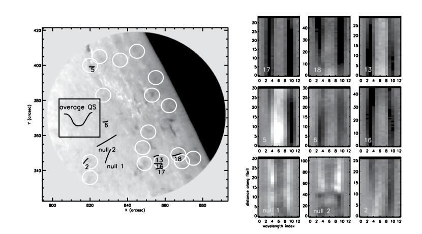
Figure 5: Left panel: an image obtained at +0.17 nm from line center in H$\alpha$ annotated with fibrils and non-fibril regions for comparison. The square shows an area of quiet Sun used to compute an average profile in H$\alpha$. The smaller panels show typical profiles (divided by the average profile) of the regions marked in the left panel, as a function of wavelength index and position along the fibril. The images have been scaled so that black corresponds to 0.7, white to 1.4 times the mean quiet Sun spectrum.

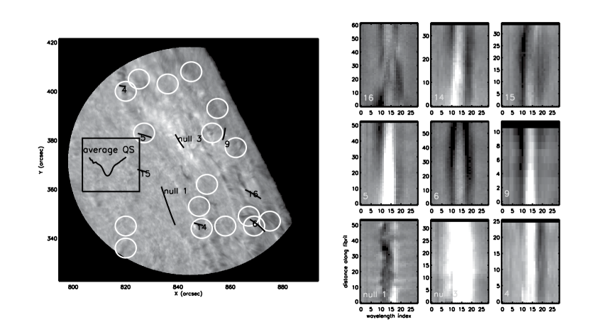
Figure 6: An identical plot to Figure 5, but for the Ca II 854.2 nm line. Fibril number 16 appears more complex- this might be due to superposition of two fibrils along the line of sight.

We identified and traced some typical fibrils visible in the wavelength scan data at 0.11 nm and 0.06 nm for H$\alpha$ and Ca II 854.2 nm respectively. We also selected a nearby region from which to derive average line profiles. The major axes of the fibrils were traced and fitted with a quadratic in the solar $x,y$ frame. Individual spectra $I_{x,p}$ were then extracted as a function of $x$ and pixel position $p$ along each fibril. Figures 5 and 6 show the fibrils selected, the regions used to calculate average spectra, $\overline{I}_{x}$, neighboring but outside of fibrils (left panels), and then the spectra $I_{x,p}/\overline{I}_{x}$. Both fibril and also some non-fibril (“null”) profiles are shown in the figures.

The fibril profiles are similar to one another yet significantly different from those of the “null” features plotted for comparison. The variations in intensity are 10-20% from fibril to non-fibril regions, the figures have color tables clipped at $80\%$ and $120\%$ of $\overline{I}_{x}$. The fibrils typically show shallower but broader absorption lines than the average profile, akin to the broad profiles described by Cauzzi et al. (2009) around magnetic network elements. Such profiles lead to a bright line core, darker near wings, and “normal” far wings clearly seen in the figure. From equation 2, this wavelength dependence of $I_{x,p}/\overline{I}_{x}$, almost symmetric around line center and similar to the second derivative of the line profile, is readily explained by fibrils having a broader line width $w$. But, of twenty such fibril profiles (not all shown), seventeen have noticeably asymmetric profiles over significant fractions of their lengths. Thus not only are fibril profiles wider but the the majority also have significant apparent velocity shifts.

In Figure 6 we show, for completeness, the profiles for Ca II fibrils, in the same fashion as for Figure 5. In the Discussion section, we examine the modest variation in these profiles as a function of distance along the fibril in an attempt assess if they are compatible with standing waves. But we warn against an over-interpretation of these profile data which, more adversely affected by residual seeing than the time series data, must be an ill-defined spatial average of actual solar profiles.

3.3 Statistics of fibrils

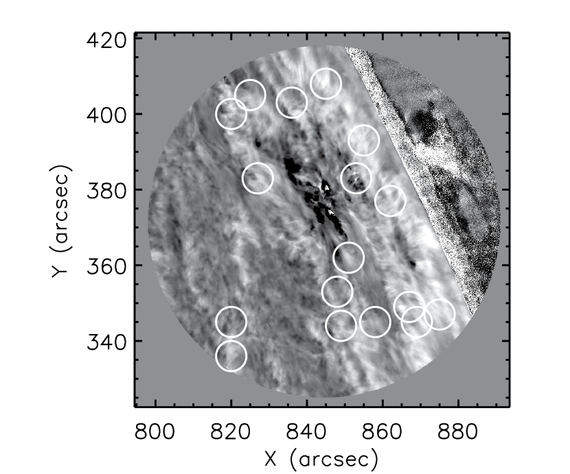
Figure 7: The image shows line widths of the Ca II 854.2 nm line computed from the first of the wavelength scans. The color table is clipped at 0.04 and 0.08 nm. This image should be compared in particular with the time averaged data of Figure 2.

In JRC12 we presented several cases of extremely rapid changes along fibrils, our objective here is to examine the statistical occurrence of such behavior. Time averaged H$\alpha$ images on the red and blue sides of the line are shown in Figure 2. Time averages are useful in highlighting “fuzzy” areas in which rapid spatial variations in fibrils are present. These areas are related to areas of enhanced line widths over the chromospheric network (Cauzzi et al., 2009). A line width image (from the first Ca II spectral scan) is shown in Figure 7. A comparison with Figure 2 reveals that the fuzzy areas are found within only some regions of enhanced line width. Thus a broad line appears a necessary but not sufficient condition for the rapid variations at 0.11 nm to be observed, consistent with the behavior of the line profiles found above. We have counted the number of detectable fibrils seen against the solar disk in sets of 40 selected blue- and 56 red-wing MFBD processed images from our sample of H$\alpha$ data. We found an average of 48 and 74 fibril-like structures per frame respectively. The distributions of the number of occurrences of finding $n$ fibrils per image are different. The area of the solar disk in the images is about 100 square degrees (in heliographic coordinates) or about 0.03 steradians, about 1/400th of the solar surface, so at any time we might find $2\times 10^{4}$ blue- and $3\times 10^{4}$ red-wing fibrils respectively, at these particular wavelengths. The sum of these numbers is within a factor of two of some estimates of numbers of type II spicules and their disk counterparts (Sekse et al., 2012).

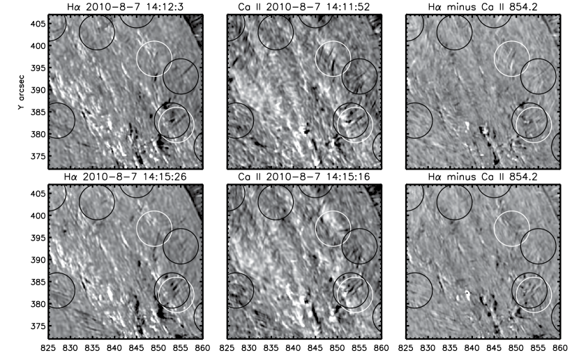
Figure 8: H$\alpha$ images at +0.11 nm and Ca II images at +0.06 nm from line center are shown in the left and middle panels respectively. The right panels show images in which the Ca II images were subtracted from H$\alpha$ images obtained just 10 sec afterwards. The white circles highlight regions where (upper right panel) fibrils appear to change from white to black along its length, indicating a continuous structure with systematically changing thermodynamic properties (line width, shift, depth) along it. In fact, close inspection reveals that this is probably a chance line-of-sight occurrence. There are very few, if any, clear cases of such continuous behavior in these data.

The data were acquired in bursts (Fig. 3), which means that fibril lifetimes, while encoded into the time series, cannot easily be determined because of burst durations are too short. The lifetimes of the observed structures appear to vary from a few tens of seconds to longer than the duration of the longest burst (100 seconds). Results discussed below (see Figure 8) show that lifetimes are probably shorter than 200 seconds.

We estimate by inspection that the fraction of fibrils exhibiting the extremely high phase speeds highlighted by JRC12 is between 1/3 and 1/6 (red wing images) and about 1/8 (blue wing). The reader can judge for his- or herself the estimate for the red wing data using online movies presented by JRC12. These small fractions do not undermine the essential arguments of JRC12, a single occurrence being sufficient to lead to the dilemma discussed by them. The majority of other fibril structures appear to evolve more slowly. Like spicules of type I they have smaller geometric aspect ratios (length/width), and include some clear examples of “coronal rain” (blobs of cool material falling out of the corona) as well as other features that appear compatible with fluid motions along tubes of magnetic flux.

3.4 Spatial relationships between blue- and red- wing fibrils

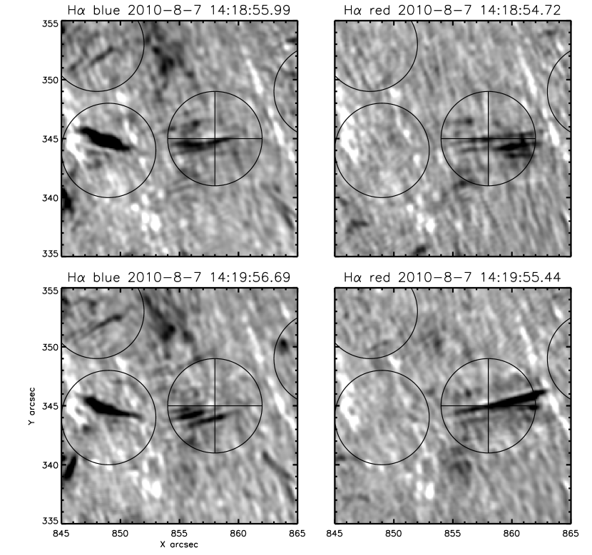
Figure 10: A close-up view of near-simultaneous H$\alpha$ blue and red wing images.($\pm 0.11$ nm). Each row contains two images obtained $\approx 1.3$ seconds apart. The lower images were taken 61 seconds after the upper images.

Our data contain several instances where a red wing image was acquired within 2 seconds of a corresponding blue image (Figure 3), for each line. Since fibril lifetimes are at least an order of magnitude larger, except for the relatively small fractions (1/8-1/3, section 3.3) of fibrils exhibiting the frame-to-frame changes highlighted by JRC12, data taken just 2 seconds apart give almost simultaneous views of the Sun at the two wavelengths (for the majority of fibrils). Figure 10 shows a typical example of the red and blue images for data taken 1.3 seconds apart, and 1 minute apart. Statistically, H$\alpha$ red images are consistently longer than those in the blue images. The $x-y$ positions of the red and blue fibrils almost never overlap, even though their axes are mostly aligned because they are rooted in clumps whose magnetic field lines appear to be part of a larger magnetic structure (e.g. Athay, 1976). In those cases when red and blue fibrils are adjacent, there is significant asymmetry between these neighboring red and blue fibril shapes (see, for example, fibrils in the cross-hairs in the figure). The fibrils immediately below the cross-hairs are in different positions in the red and blue images. Those neighboring frames at different wavelengths in the Ca II time series data show qualitatively similar results, except that the fibrils’ lengths are not noticeably different in the red vs blue sides of the Ca II lines.

In summary, close examination shows that red- and blue- wing fibrils can be found that are sometimes co-spatial and often parallel. Indeed they must be co-spatial for the small fraction of fibrils showing almost symmetric profiles (section 3.2). However, the majority of the spectra appear asymmetric. Consequently the majority of fibrils are not co-spatial. If, as some have suggested (De Pontieu et al., 2012), torsional motion is important, we should see evidence for this in our data instead. Those red and blue fibrils which appear parallel (compare the cross-hair images) have morphologies that are very different in the red and blue wing data. The significance of this finding is discussed in section 4.3.

3.5 Comparison of H$\alpha$ and Ca II 854.2nm data

Our time series dataset contains several instances where Ca II images were acquired within 10 seconds of H$\alpha$ images. The Ca II images were taken at $\pm 0.06$ nm (equivalent to a Doppler shift of 21  km s^-1) compared with $\pm 0.11$ nm (50  km s^-1) for H$\alpha$. The interpretation of these data is generally complicated not only by the non-LTE formation of the lines through the dependence on absorption strength on $n_{i}$ (Athay, 1976), but also by the fact that the observability of fibrils depends on both line widths and flow speeds (see our equation 1). Nevertheless we can make a simple hypothesis and test it using the parametric model of line formation of section 3.1.

Some authors (e.g. De Pontieu et al., 2009, 2011) have suggested that chromospheric plasma is accelerated and heated along fibril tubes to some 50 -100  km s^-1. Let us assume that flows along tubes occur (whether accelerated, decelerated or constant). How would such flows be manifested in a comparison of H$\alpha$ and Ca II data at +0.11 and +0.06 nm? In the line cores there is much confusion in the images making such a comparison difficult. However, in the cleaner wing images, even though they are acquired at significantly different equivalent Doppler shifts (50 vs. 21 km/s), we might expect to see evidence of simply connected flows using the two lines, if they are present. The thermal properties of the two lines (excitation energies, line widths) are somewhat different. but chromospheric plasma is dense enough that momentum changing collisions between atomic species rapidly drives dissimilar bulk velocities to zero (making $s$ and non-thermal contributions to $w$ similar for H and Ca). Thermal line widths and $n_{i}\Delta$ are very different for the lines, so we certainly do not expect to see one-to-one correlations. But we should be able to find at least some clear examples where a dark feature seen in the Ca II line co-aligns with a dark feature in H$\alpha$.

To search for flow signatures in fibrils we co-registered (to sub-pixel accuracy) and subtracted Ca II images from H$\alpha$ images, for three cases where data taken close in time (10 sec apart) are available. Results for two cases are shown in Figure 8. The two left columns are speckle reconstructed images at +0.11 and +0.06 nm respectively for H$\alpha$ and Ca II 854.2 nm. The second row contains data obtained some $\approx 200$ sec apart. Two properties are clear from these images: first, essentially no fibril structures are the same between 14:12:03 UT and 14:15:26 UT- the lifetimes of the observed fibrils is less than 200s. Second, although some features appear common to both H$\alpha$ and Ca II data, most of the time the H$\alpha$ and Ca II fibrils are spatially separate from one another, even though at a lower angular resolution ($\approx 1\arcsec$, say) one might conclude that arise from one and the same feature. (Fibrils in the lower of the two circles are examples). To account for an offset of say $0\farcs 5$ by real lateral motion of fibrils would require physical velocities $\mathrel{\hbox to0.0pt{\lower 3.5pt\hbox{$\sim$}\hss}\raise 1.5pt\hbox{$>$}}36$  km s^-1. Such displacements would be visible in the difference image (rightmost column) as black and white features aligned along the fibril lengths. The lower circle includes one such possible feature. But most of the black/white adjacent features in fact correspond to differences in brightness of faculae and remain present in both sets of data separated by 200s (see the region near $x,y=836\arcsec,393\arcsec$).

The difference images (rightmost panels in Figure 8) can also reveal plasma accelerations, which in the model are $ds/d\ell$ which would be manifested as fibrils that show a moving absorption along their lengths $\ell$. Our angular resolution $\sim 0\farcs 2$ corresponds to about 150 km on the Sun, so it is not unreasonable to expect to see evidence of plasma acceleration along a typical fibril of length $5\arcsec{}\equiv 3500$ km, if it is common. The thermal properties and the particular acceleration profile will determine exactly where along a given flux tube the absorption will occur in both lines. Therefore we expect to observe a variety of bright and dark features aligned along a tube in such images. If part of a simply accelerated tube of plasma, their axes must be precisely aligned in the very narrow, essentially unresolved fibrils. Remarkably, there are very few clear examples which might correspond to accelerated plasma (Figure 8). The upper circled region shows an example of an almost co-aligned transition from dark to light in the rightmost upper image. Close inspection reveals that the dark and light regions are not precisely co-axial, so those observed seem to appear by chance. We have found no convincing case in our dataset, a factor of 70 less than the total number of fibrils observed.

We estimate the likelihood that such alignments occur by chance. Fibrils occur in groups within which they tend to follow the direction of their neighbors (refer to any IBIS image in the present paper). We imagine dropping a “Ca fibril” of length $5\arcsec$ (50 pixels) onto a given fibril clump seen in H$\alpha$. Assume that one H$\alpha$ fibril lies along a line between $x=0$ and $x=5\arcsec$. The base area of the fibril group appears to be on the order of $A\sim 25$ square seconds of arc (Figure 2), from which $\sim 10$ fibrils originate. The chance of finding one “Ca fibril” with either end point within an area $a$ of 1 pixel by 1$\arcsec$ ($a=0\farcs 1^{2}$), at either $x=0$ or $x=5$, is roughly $P_{1}=4a/A\sim 0.02$. If fibrils have azimuthal distributions within a group with a width of say 0.2 radians, only a fraction $P_{2}=b/0.2$ will appear sufficiently aligned with the H$\alpha$ fibril. For $b$ we use one half of the ratio of fibril width/length, $b\sim 1/20$. The net probability for finding one coincidence at random is then roughly $P=n\times nP_{1}P_{2}$ in one group which contains $n=10$ Ca and $n=10$ H fibrils, or $P=0.4$. With the $\sim 10$ groups in the FOV (Figure 2) we expect to see at $\sim 4$ coincidences across the observed field of view at any given time. Given the roughness of these estimates, we conclude that the lack of an observed relationship between the Ca II and H$\alpha$ fibrils, seen at 0.06 and then 0.11 nm respectively, is consistent with the null hypothesis. No fibrils are detected above the number expected from a random alignment of Ca II and H$\alpha$ fibrils.

Lastly, we made further comparisons of the H$\alpha$ and Ca II lines from the wavelength scans. The time series datasets analyzed below and by JRC12 were obtained mostly at $\pm 0.11$ nm in H$\alpha$, $\pm 0.06$ nm in Ca II (see Figure 3). From the wavelength scans we compared first H$\alpha$ data at -0.103 nm to Ca II images taken at -0.136 nm, i.e. at the same Doppler shift of $\approx 47$  km s^-1. Each set of H$\alpha$ and Ca II images were taken within 7 seconds of each other and were co-aligned. The fibrils observed in the H$\alpha$ images are absent in Ca II images at this same Doppler shift. It seems likely that the optical depth $\delta\tau_{x}$ in the Ca II lines must be smaller than that of H$\alpha$ in the structures leading to the H$\alpha$ fibrils. Thermal broadening can in part explain this difference (Cauzzi et al., 2009), since for hydrogen lines when $T_{ion}\sim 2\times 10^{4}$K, thermal broadening is on the order of $w\approx 12$  km s^-1, 1/4 of the observed values of 47  km s^-1. There may also exist a contribution from the different thermodynamic states of hydrogen and calcium in the fibril plasma that determine $n_{i}$ (see e.g. Athay, 1976), but in section 4.2 we find that variations in $n_{i}\Delta$ are important only for the Ca II line.

3.6 Relationship of the fibrils to chromosphere, transition region and corona

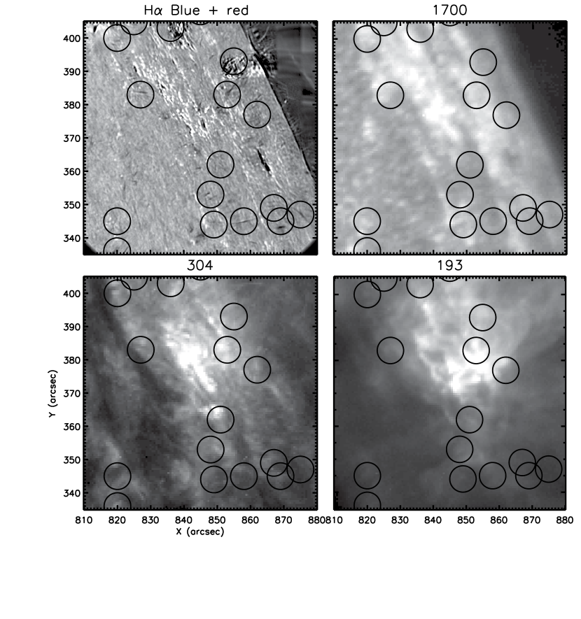
Figure 9: A comparison of IBIS fibrils (groups are encircled, taken from Figure 2) with data from the AIA instrument on SDO obtained between 14:25:19 and 14:25:31 UT on August 7 2010.

Figure 9 shows the spatial relationship between the H$\alpha$ wing fibrils and data of the low chromosphere (160 nm), transition region (30.4 nm) and corona (19.3 nm) as seen with the AIA instrument on SDO. AIA’s angular resolution of 1$\farcs$5 is 7 times lower than the resolution of IBIS. Importantly, 1$\farcs$5 exceeds the widths of many of IBIS fibrils by a factor of several. Thus we can compare SDO and IBIS images only at course angular resolutions. Earlier figures and Figure 9 shows that these wing fibrils originate from bright patches in the chromospheric network, a well documented result (e.g. Athay, 1976). As such, they are also grouped largely over the network where the 30.4 nm emission in He II is also brighter, as helium emission is associated with the chromospheric network (Jordan, 1975, e.g.). While no 1:1 relationship with He II is expected (e.g., Pietarila and Judge, 2004, and references therein), clearly both the fibrils and 30.4 nm emission originate in network regions. In stark contrast, the coronal emission is confined largely to active region loops anchored in and around the sunspots. Whatever the physical process is that generates the fibrils observed in the wings of H$\alpha$ and Ca II, it has no detectable counterpart in the corona at this spatial resolution. Any correlation with the He II image at 30.4 nm, although stronger, is still very weak: the lower left panel of Figure 9 has fibril circles always with moderately bright He II emission, but there are many such bright regions with no fibrils.

If the H$\alpha$ fibrils are directly correlated with Type II spicules, it is difficult to reconcile the idea that the fibrils observed here have much to do with the supply of mass, momentum and energy into the corona (cf. De Pontieu et al., 2009, see the Discussion below).

4 Discussion

4.1 New observational results

In summary:

• At any time there are $\sim 120$ fibril-like structures seen at $\pm 0.11$nm either side of H$\alpha$ line center in the IBIS FOV. If covering the entire Sun there would be a total of $5\times 10^{4}$ fibrils.

• Of these, one in five exhibit the very rapid changes reported earlier (JRC12).

• The statistics of blue vs red wing data ($\pm 0.11$nm) of H$\alpha$ are different in this particular limb region. The center of the IBIS frames has a line-of-sight that is at $\vartheta_{C}=78^{\circ}$ to the local vertical on the Sun, so that horizontal flows yield higher fibril visibilities in the line wings than vertical flows of the same magnitude through Doppler shifts $s$ in equation 1.

• The fibrils seen in red- and blue- wings in H$\alpha$ appear in the same regions of network with enhanced line widths, but they are spatially and temporally distinct.

• Near-simultaneous Ca II and H$\alpha$ data obtained at different Doppler shifts (20 and 50  km s^-1 respectively) reveal no clear examples of acceleration along the length of a fibril, of some 70 statistically independent cases. These statistics are consistent with chance alignment of fibrils seen in Ca II and H$\alpha$ data.

• The wavelength scans of H$\alpha$, although containing significantly more residual atmospheric seeing, nevertheless show that fibril profiles statistically are broader, shallower and more asymmetric than the mean profile. The red- and blue-wing fibrils occur in areas of broad H$\alpha$ and Ca II line profiles, they are pervasive around magnetic concentrations.

• The red- and blue-wing fibrils seen in the reconstructed images occur in areas that are correlated to bright UV/EUV emission from the chromosphere and transition region seen at a lower resolution from space. We could find no correlations with the brightness of the overlying corona.

4.2 Interpretation of line wing images

The line profiles can be examined in the light of the simple model of section 3.1. Figures 5 and 6 show images of fibril profiles divided by the average profile $r_{x,p}=I_{x,p}/\overline{I}_{x}$. The data shown, the first of their respective scans, are typical. If we adopt $\overline{I}_{x}$ as the profile in the absence of overlying fibril absorption, then with equation (1), $r_{x,p}=1+\delta I_{x,p}/\overline{I}_{x}$. The striking vertically banded structure seen in these Figures is common to all fibrils, it stands in contrast to the two non-fibril (“null”) cases also shown. A few fibril profiles are almost symmetric around line center. In the model, these profiles correspond to terms proportional to $\partial^{2}\phi_{x}/\partial x^{2}$ (see the fibril with index 17, for example), which therefore correspond to changes in the line widths $w$.

The majority of fibrils, however, show profiles proportional to the first derivative as well. Some of these profiles change along the fibril length as the two derivative components compete for dominance (see those labeled 2 and 5 for example), indicative of acceleration or deceleration ($ds/d\ell\neq 0$ as a function of distance $\ell$ along the fibril length). Thus we conclude that most fibrils, as measured using these seeing-influenced data, are broader and Doppler shifted relative to the average profile.

To extract more information contained in these profile ratios $r_{x,p}$, we have applied Principal Component Analysis (“PCA”, e.g. Jolliffe, 2002) to the spectra. PCA reveals the patterns present in the data and their relative frequencies of occurrence. For each pixel $p$ the vector ($r_{x,p}$) was constructed as a function of frequency $x$, and the vectors over all pixels were averaged. The outer product of this average vector was computed along with eigenvalues and eigenvectors of the derived matrix. Results of PCA of the H$\alpha$ fibril profiles are shown in Figure 11. The eigenvalue spectrum drops to less than 1% after the first four components. The same plot for the null pixels (not shown) is far steeper, dropping to 0.01% in the first four components. The eigenvectors with smaller eigenvalues have more noise, judging by the higher frequency variations. The data are therefore represented adequately (i.e. above noise levels) by a few principal components. The figure shows the average profile $I_{x}$ and the eigenvectors of the first six components of the ratio of $I_{x}$ to this average profile. We recognize vectors 1 and 2 as second order-like component ($\partial^{2}\phi_{x}/\partial x^{2}$), and vectors 3 and 4 as first order-like components. Higher order vectors 5 and 6 are associated with noise or systematic errors. Vector 1 is a combination of a DC offset and a second order-like profile, appearing similar to the average $\delta I_{x}$ profile. An offset (i.e., eigenvector independent of wavelength index on the abscissae) reflects changes independent of wavelength in the dataset- these are simple brightness variations of the photosphere underlying the fibrils.

The PCA analysis therefore confirms that the H$\alpha$ fibril ratios $r_{x,p}$ therefore are dominated by a linear combination of the zeroth, first and second derivatives of the line profiles with wavelength. According to our model, the H$\alpha$ fibril properties involve variations in all three parameters: brightness, line shift and line width. The null profiles are similar but the eigenvalues of vectors 2,3,4… are all 0.1% or smaller- i.e. the occurrences of variations attributable to line widths and shifts are far smaller.

Figure 12 shows the same plot but for Ca II fibrils. These have a similar eigenvalue spectrum to H$\alpha$ but the first two eigenvectors appear similar to $\phi_{x}$, i.e. the brightness or zeroth derivative of the profile. A mix of first and second order derivatives are in components 3 and 4 with eigenvalues 0.05 and 0.03 respectively. Thus, the Ca II fibril variations correspond, in the model, first to changes in column density $n_{i}\Delta$, second to changes in line width $w$ and third changes in line shift $s$ respectively.

It is important to note that the lack of spatial correspondence between the red and blue fibril images (section 3.4) results primarily from the asymmetry induced by changes in $s$.

4.3 Our work in context: Phenomenology

The combination of high cadence, high spectral and angular resolution of our chromospheric data approaches the limit of modern instrumentation, and comparable datasets are still few and far between (Table 1). Early literature on spicules is important but was based on observations with smaller ground-based telescopes in the era before adaptive optics and image processing were available (Roberts, 1945; Beckers, 1968, 1972). Such early studies would not have detected the fine structures examined here (Pereira et al., 2013, see also our Appendix B). To date, space-based data (e.g. de Pontieu et al., 2007) have been obtained with slower cadences at single wavelengths and in broader bandpasses than reported here. Modern ground-based work has usually emphasized image quality at the expense of high cadence (Table 1).

Rutten (2006, 2007) reported very fine “straws” as long, bright and rapidly evolving features seen near the limb in broadband Ca II H images from the Dutch Open Telescope. Using data from Hinode, again in broadband Ca II H images, de Pontieu et al. (2007) reported two types – at least – of limb spicules. The “type I” spicules have been identified with the dynamic fibrils seen on disk and explained as shock-driven plasma undergoing an upward-downward motion cycle (Hansteen et al., 2006), while the “type II” spicules had many similarities with the “straws”, including a very large aspect ratio (widths of a few hundred km, lengths up to several Mm), a short lifetime (10-150 s), and large amplitude swaying presumably induced by pervasive Alfvén waves in the chromosphere. Several groups have tried to identify these features on the solar disk, concluding that they correspond to “rapidly blue-shifted excursions” (RBEs) in H$\alpha$ and Ca II 854.2 nm profiles, seen as blue-ward absorption components in disk spectra (Langangen et al., 2008; Rouppe van der Voort et al., 2009; Sekse et al., 2012). From their derived Doppler velocities and widths, these RBEs displayed a trend of acceleration and heating from their foot-points (in the magnetic network) upwards.

By early 2012 the combination of type II spicules, RBEs, and some EUV observations from space (De Pontieu et al., 2009, 2011) comprised an apparently coherent picture of chromospheric plasma undergoing heating and flowing into the corona in tube-like structures. (However, in view of the large flux-tube expansion with height, it still remained unclear how such plasma features could appear so collimated so high above the solar surface, see JRC2012). The story continues with the recent report of data (De Pontieu et al., 2012) which apparently need yet another kind of motion within the spicules, namely a torsional motion, in order to explain the observed slope of spectral lines at the limb. Expanding on this idea, and re-analyzing some of the same datasets used in earlier works, Sekse et al. (2013b) highlighted “rapid redshifted excursions” (RREs) in H$\alpha$ and Ca II 854.2 nm profiles seen close to disk center, with an occurrence about half that of RBEs. Sekse et al. (2013b) claim that “the striking similarity of RREs to RBEs implies that RREs are a manifestation of the same physical phenomenon”. As some RRE and RBE pairs appear adjacent to one another, these authors interpret such neighboring signatures as further evidence for torsional, vortex flows inside tubes.

To explain the behavior seen in the light of all these new datasets of fibrils, the traditional picture of plasma flows in a tube apparently requires an increasingly complex array of physical processes taking place within it, including outflow; heating; tube waves; reflection of tube waves to produce standing waves (Okamoto and De Pontieu, 2011); vortex-like rotational motion (De Pontieu et al., 2012; Sekse et al., 2013b). Even so, it must be remarked that some of the RBEs/RREs characteristics observed in recent high quality data sets (apart from our own) are objectively difficult to accommodate into this picture: Fig. 4 of Sekse et al. (2013b) for example shows that a large fraction of fibrils around a network patch displays larger Doppler velocities and widths towards their footprints, quite contrary to what required by the acceleration scenario. Even if swaying and/or torsional motions are present within the fibrils, the large spatial coherence of such flows (7-10,000 km in the horizontal direction, i.e. along a string of network points) would require an organized collective behavior wholly unexpected from first principles. Further, while the presence of RRE and RBE pairs adjacent to one another can certainly indicate torsional motions (which were hypothesized in spicules already by Beckers, 1968), it also implies that the horizontal extension of these fibrils is quite larger than usually assumed when looking at a single wavelength. The several examples displayed in Figs. 2, 8 and 9 of Sekse et al. (2013b) all suggest that the fibrils involved have a width of 1 arcsec or even larger, which runs contrary to the original definition of type II spicules (de Pontieu et al., 2007).

How do these pictures relate to our data? If we assume that torsional motions are responsible for observed close and near-parallel pairs of red and blue wing images (Figure 10), then the data presented here show that conditions must be systematically different for the blue-ward and red-ward components of this torsional motion. If separated by a distance of $\ell\sim 200$ km (see the parallel but offset red- and blue-wing data in the cross-hairs of Figure 10), the Alfvén crossing time between sides of the vortex would be a few seconds (assuming a low $\beta$ plasma and $C^{2}_{A}\sim C^{2}_{S}/\beta$). This time is short compared with the lifetimes of most fibrils examined, so that a combination of MHD waves and rotational motion (with velocities $\mathrel{\hbox to0.0pt{\lower 3.5pt\hbox{$\sim$}\hss}\raise 1.5pt\hbox{$<$}}C_{A}$) might be expected to produce more symmetric pairs of fibrils than we observe, as the same material flows around the vortex becoming visible in both red and blue images.

Given this rapidly evolving literature, we can only speculate how our data might really fit into it. On the one hand, the statistics, appearance, lifetime of the fibrils presented in this paper suggest that we are observing RBEs and RREs and/or type II spicules, close to the limb on the solar disk. Yet, several other characteristics do not fit with the pictures proposed in the work cited above. For example, we rarely observe clear cases of side by side blue/red fibrils (which could evidence vortex-like motions), and for the few cases in which we do, we also observe a significant spatial asymmetry in the blue/red images along the fibrils’ length, something not reported by Sekse et al. (2013b). Further, we do not find a clear relationship between Ca II 854.2 nm and H$\alpha$ fibrils in the sense highlighted by Sekse et al. (2012), i.e. that “Ca II 8542 RBEs are connected to H$\alpha$ RBEs and are located closer to the network regions with the H$\alpha$ RBEs being a continuation of the Ca II 8542 RBEs”. Certainly our data, obtained close to the solar limb, favor detection of horizontal motions that can induce line shifts, but this observational bias should not be of any relevance for the detection of torsional motions within a (mostly) vertical tube, or of accelerated plasma progressively appearing at larger heights in projection, if present (Sect. 3.5).

We have no explanation for these discrepancies, and just note that the interpretation of data revealing chromospheric “fibrils” remains rather confused. We suggest that the analysis of full spectral profiles at the highest cadence and spatial resolution should be the highest priority of future research: as we showed in Sect. 3.2, the fibrils’ profiles are most often broadened with respect to the “quiet” areas around them, a result consistent with older literature (e.g., Athay, 1976) and with the findings of Cauzzi et al. (2009). Intensity changes at any given wavelength (or few wing wavelengths) will depend on the original profiles (Sect. 3.1) so that interpretation only in terms on separate red and blue “components” (e.g. Rouppe van der Voort et al., 2009; Sekse et al., 2013b) might be subject to bias. In our spectral scans we find from PCA analysis of line profiles that the origins of variations in H$\alpha$ that lead to wing fibrils (and hence RBEs, RREs etc) are, to leading order, dependent on the Doppler shifts and widths.

4.4 Conjectures and Refutations

How can we then proceed, given the bewildering array of observational facts summarized above? In this paper we seek to disprove hypotheses - the approach advocated by (Popper, 1972, “Conjectures and refutations” is a famous monograph by Popper). Most work on chromospheric fine structure has not explicitly sought to do this. While far more mundane, than, say, the persistent precession of Mercury’s orbit, highlighted by Le Verrier and which refused to agree with Newtonian theory, JRC12 presented data whose essential properties required some improbable mental gymnastics to make them fit into the tube model. We therefore appealed to sheets as an alternative physically plausible hypothesis needed to explain critical aspects of the data, to be tested further.

The reader might justifiably adopt “Occam’s Razor” and accept the “simplest answer compatible with the data”. But there is a problem: what actually is the simplest answer for chromospheric fine structure, given, for example, that there is no explanation even for the extraordinarily large aspect ratios found? Let us consider the two cases physically, putting aside briefly the data presented by JRC12:

• The tube picture is a natural choice because the observed phenomena certainly appear like thin straws, and the electrically conducting plasma (partially or fully ionized) is frozen to tubes of magnetic flux on observable scales. But magnetic structure rooted at the network photosphere boundary appears mostly like rivers not isolated tubes (JTL11- see the references therein). Also, there is as yet no straightforward explanation for the formation of such thin structures (aspect ratios $>10-20$) that do not measurably expand with height within the chromosphere.

• The sheet picture was prompted through consideration of ribbon-like observed photospheric network magnetic structure, of interfaces between bundles of flux (van Ballegooijen et al., 1998; Priest et al., 2002) and of Parker’s theory of the formation of TDs. In the latter, thin sheet-like structures are predicted to originate simply because force balance and magnetic topology are not generally consistent with continuous solutions for the magnetic field (Parker, 1994). They are weak solutions to the governing partial differential equations similar to shocks so familiar in continuum fluid mechanics. The magnetic field direction, but not magnitude, changes slightly across flux surfaces. The apparent width of plasma embedded in sheets can readily be below observable scales (appendix B), so that the visible warps in sheets do not need to expand with height as tubes of potential fields must do.

4.5 Data vs models and some physical implications

.

The idea that spicules supply mass, momentum, and energy to the corona is at least 65 years old (Thomas, 1948; Miyamoto, 1949; Pneuman and Kopp, 1978; Athay and Holzer, 1982). Naturally, spicules of type II, which share qualitative similarities of upward apparent motion and fading (Pereira et al., 2013) with the “classical” spicules reviewed by Beckers (1968), continue to draw attention as a manifestation of mass and energy supply to the corona. Much recent work has used spacecraft data from chromosphere to corona to support this picture (de Pontieu et al., 2007; De Pontieu et al., 2009, 2011). As such, essentially all workers interpret the data found in terms of the motion (flows and wave motion) in elemental tubes of plasma frozen to magnetic lines of force. Do our data allow us to try to falsify this or the sheet-like proposition discussed in the Introduction?

If, as appears reasonable, we are observing the near-limb counterparts of RREs, RBEs and type II spicules, the lack of spatial (let alone temporal) correlation between the fibrils and the overlying coronal emission is striking and important. Either the particular features we are observing are unrelated to those that have been reported to accelerate heated plasma into the corona (e.g. De Pontieu et al., 2009, 2011), being a separate, mostly horizontal population of fibrils/spicules, or the acceleration proposal needs further examination.

It is critical to the “tube” hypothesis that standing waves account for the very fast phase speeds we have reported. Can we reject the hypothesis that the standing-wave scenario explains the data we have reported here and earlier, without reference to the many other studies? In JRC12 we dismissed standing waves for the particular behavior found in that paper because complete fibrils appeared out of nowhere, with no evidence of the setting up of a standing wave from the interaction of two propagating waves. In appendix A we review these and other problems with standing waves. But the standing wave scenario can, in fact, indeed be rejected for our data. One primary characteristic of the time series measured in one very narrow spectral band is that the absorbing intensities are remarkably uniform along the entire length of the fibrils (see the figures in JRC12). If wave motions were responsible, the kink/helical waveforms would have Doppler shifts that depend on position along the tube, having nodes and antinodes somewhere along their length. This must translate, for a harmonic wave, to absorption features which track in space loci where Doppler shifts match the observed bandpass- we should observe evidence of this nodal structure along the fibril length. The calculations of section 3.1 show just how sensitive the intensities can be to small, subsonic changes in line shift and width parameters. But we do not observe the gradients of intensity in these fibrils that would correspond to the necessary varying velocities of plasma organized in standing waves. While tubular in appearance, the fact that we fail to observe a critical component of the flux tube model- the standing waves of plasma that supposedly travel along these flux tubes- discredits the picture.

Can we then reject sheets? For spicules of “type I” there is no debate (and never has been). We know of no data that contradict the model predictions of Hansteen et al. (2006), so a new hypothesis is not warranted there. However, unlike Pereira et al. (2012), we believe that evidence could and can be found against the sheet hypothesis with current instrumentation (see Appendix C). Two critical tests would serve to reject sheets.

First is the observation that “type II spicules” appear only to travel upwards. Time reversal applied to a harmonically varying sheet such as shown in JTL2011 means that as many fibrils (if sheets in projection) will move down as well as up. The type II spicule cannot therefore be such a simple sheet. In JTL2011 we noted that sheets will tend to be driven by forces below them. Perturbations from below propagate up in the form of Alfvénic disturbances. In order to break the time reversal symmetry there must be some hysteresis in these motions. Alfvén waves are naturally damped by ion-neutral collisions, an irreversible process that breaks this symmetry. Such effects may also account for some heating of chromospheric plasma. It remains to be seen the magnitude of this effect, it may prove sufficient to reject the sheet hypothesis in some fibrils, in the absence of the needed stereoscopic data.

Second, if imaging spectroscopy proves that vortex motions in these magnetically dominated plasmas are the rule, as reflected in the observation of parallel pairs of blue- and red- shifted fibrils (Sekse et al., 2013b) Occam’s Razor would suggest that some rotational symmetry is required. This is not expected to be a common form for tangential discontinuities formed as anticipated in the spontaneous or tectonic pictures. While “solar tornadoes” have been found stereoscopically in much larger structures in the corona (Nisticò et al., 2009), fibril observations so far have shown that adjacent, parallel fibrils have Doppler shifts that might be vortices. However, as we noted (section 4.3), the red and blue motions are spatially asymmetric, and, by enlarging the foot-point area we see that they have a good chance of being adjacent, unrelated flows (see the calculation of chance occurrences of seeing continuous jets in Section 3.5). In the absence of shocks and embedded tangential discontinuities, vortices demand a steady gradient in speed as a function of distance from the vortex axis. Detection of the full profile of vortices for a given observation would serve to reject the sheet picture for the underlying structure. This has not been demonstrated.

What is the physical meaning of the relationship between the fibrils we observed and the emission from the chromosphere, transition region and corona shown in Figure 9? If, as argued by several authors (e.g. De Pontieu et al., 2009), there is a relationship between type II spicules and the supply of mass and energy to the overlying corona, we should see at least some correlation of the occurrence of the fibrils with the overlying coronal emission. No such correlation exists in our data, even though our data span over 30 minutes which is roughly the cooling time of the overlying corona. Also, we are not convinced by the analysis of De Pontieu et al. (2011) who correlate various fibrils and spicules of type II with lower angular resolution, broad-band SDO data. In particular the connections to the corona are very unclear, and He II 30.4 nm emission is not understood (Pietarila and Judge, 2004; Judge and Pietarila, 2004). In our data the fibrils are correlated with chromospheric network including emission in He II. But there is much He II emission outside of the areas where we observe many fibrils (circled regions in the figures). Such a correlation, even if it did exist, does not require volumetric heating of the form implied by de Pontieu et al., since alternative explanations involving cross-field particle and heat transport from the corona to the cooler spicular material have not yet been rejected (Athay, 1990; Judge, 2008). In fact, the smooth tailing off of intensity in the type II spicules with height might be accounted for naturally in such scenarios. Even more surprising, if the mechanisms discussed by Athay (1990); Judge (2008) are important, energy is transferred from the corona to the chromospheric plasma- precisely the opposite of the proposition of De Pontieu et al. (2009)!

Lastly, at the risk of precipitating a non-productive discussion, we feel we must comment on some relevant criticisms of our recent work. We do this in appendices A,B and C. The first Appendix casts a critical eye on the proposal that standing waves are a credible explanation for the fast phase speeds reported by JRC12. The second discusses physical lower limits to the scales across spicules in the light of work by Pereira et al. (2013). The third comments on a subsection of a paper entitled “are spicules sheets” (Pereira et al., 2013). It is hoped that the debate can and will end by the rejection of a model when it fails to reproduce critical data. The sudden appearance along the entire length of fibrils reported in JRC12, augmented with the present analysis, suffices to reject tube waves as a plausible explanation for the significant fraction (one in five) of fibrils evident in our data.

4.6 Implications for future chromospheric observations

Our results extend the broad (but, to us at least, confusing) literature which reports very rapid evolution of chromospheric structures consisting of narrow elongated structures variously called fibrils, mottles, spicules, spicules of type II, RBEs, now RREs, jets, even “cool loops” (e.g. Athay, 1976; de Pontieu et al., 2007; Rouppe van der Voort et al., 2009; de Wijn, 2012; Judge and Centeno, 2008; Sasso et al., 2012; Sekse et al., 2013b). To understand the real origin and importance of these structures it seems profitable to pursue the highest possible cadence imaging spectroscopy of the Sun. IBIS is one of several ground-based Fabry-Perot instruments that can observe large, circular areas of the Sun ($\sim 10^{4}$ square arcseconds) with useful reconstructed data at 1Hz, centered at a single wavelength and a very high ($R=250,000)$ spectral resolution. This stands in contrast to existing space-based instrumentation. IRIS is the latest generation of UV “imaging spectrographs” in which a slit is rastered rapidly to generate images. The two techniques are complementary. Given our data, we choose 5 seconds as an upper limit to the cadence for obtaining (almost) seeing-free spectral images. We also need a field of view spanning roughly $10\arcsec\times 10\arcsec$ to see complete fibrils which are oriented independently of any instrumental detector. How do these two instrument configurations match up to these constraints? Consider:

• IBIS could obtain five wavelengths across a spectral line in bursts of ten 0.1s exposures, and obtain 100 such areas. If polarimetry were needed, the cadence would decrease to 20 seconds for the same conditions.

• In the same time IRIS could acquire far richer set of UV spectral data, but the area covered is limited to $n\sim 10^{2}$ square arc seconds where $n$ is the raster step size. Since $n\sim 10$ is needed to cover an area of width $3\arcsec$ with $0\farcs 3$ steps, it is clear that $n\sim 30$ is needed. Each step will typically require 1s. Slit-based instruments actually are not ideally suited to the study of the thin, dynamic fibril structures which have lengths of 5 seconds of arc and which are fractions of an arc second across.

Thus, a combination of imaging and slit spectroscopy is required. Both are available now. Both should be used to challenge proposed physical pictures of fibrils.

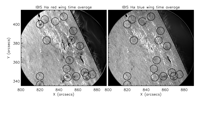
Figure 2: The time average of images obtained 0.11 nm on the red (left) and blue (right) sides of H$\alpha$ line center, from IBIS. 292 red images obtained between 14:11 and 14:34 UT, and 90 blue images were obtained between 14:15 and 14:23 UT, each reconstructed using multi-frame blind deconvolution, were used to construct this figure. A linear color table was used between the 5% and 95% levels in the distributions of brightness. “Blurred” features are rapidly moving chromospheric fine structures, including some analyzed by JRC12. Photospheric features (sunspots, plages) are much sharper. The circles highlight regions where properties of fibrils are examined in this paper. These encircled regions appear in other figures.

Figure 3: A figure showing the final set of fully processed intensity data acquired with the IBIS instrument on 7th August 2010. The times and wavelengths of the “monochromatic” images (with a spectral resolution of 200,000) in lines of H$\alpha$ and of Ca II at 854.2 nm are shown as a function of time. The data marked “JRC12” is the 100-frame 1 sec cadence dataset analyzed by Judge et al. (2012).

Figure 11: PCA decomposition of the fibril spectra in the H$\alpha$ line. The top left panel shows the distribution of eigenvalues, the mid top panel shows a normalized average profile for the fibrils, and the others show the eigenvectors that belong to the principal components. The wavelength scales are shown in the average profile panel. The y axis scales on the eigenvector components are linear but arbitrary, it is only the form of the profiles that is important.

Figure 12: PCA decomposition of the fibril spectra in the Ca II 854.2 nm line.

Table 1: The evolution of spicule and fibril spectral imaging observations

Reference	Line(s)[$n\lambda$]	${\cal R}=\lambda/\Delta\lambda$	Spatial	Cadence
			resolution
Beckers (1968)	H$\alpha$ / various	$2000-20\,000$	$\approx 1-2\arcsec$	$\mathrel{\hbox to0.0pt{\lower 3.5pt\hbox{$\sim$}\hss}\raise 1.5pt\hbox{$>$}}4$ sec
Rutten (2006)	Ca II 396.8[1]	2800	0$\farcs$2	$\approx 10$ sec
de Pontieu et al. (2007)	Ca II 396.8[1]	1800	$0\farcs 16$	$\geq 4$ sec
Judge et al. (2012)	H$\alpha$[1]	$250\,000$	$0\farcs 2$	1 sec
Sekse et al. (2012)	Ca II 854.2[16] H$\alpha$[28]	100 000	0$\farcs$18, 0$\farcs$14	12 sec
Sekse et al. (2013a)	H$\alpha$[4-35]	100 000	0$\farcs$14	0.9-8 sec
Sekse et al. (2013b)	Ca II 854.2, H$\alpha$	100 000	0$\farcs$18,0$\farcs$14	various
This paper	H$\alpha$[1], Ca II 854.2[1]	$250\,000$	$0\farcs 17,0\farcs 22$	1, 5 sec
	H$\alpha$[13], Ca II 854.2[29]	$250\,000$	$>0\farcs 2$	15 sec

Note. —

Appendix A Standing waves and spicules

Sekse et al. (2013a) cite Okamoto and De Pontieu (2011) (henceforth “OdP2011”) as providing “conclusive” evidence that standing waves are an acceptable explanation of rapid changes seen along the lengths of spicules. Let us critically examine this claim, first as applied to their data, and then in reference to our data.

OdP2011 analyzed a time series of limb data of a coronal hole boundary in the Ca II H line with the 0.3 nm-wide filter of the SOT instrument on the Hinode satellite. They average 1.6s exposures over 9 frames for a cadence of 14s. Unspecified radial density gradient and spatial high pass filters were applied. Their algorithm finds bright features in the time-averaged time series that are persistent in time ($>45$s lifetime) and space (30 pixel overlap of the feature’s long axis between frames), long ($>8\arcsec$ at its maximum), have weak curvature ($<5^{\circ}$ over lengths of 4$\arcsec$). They identified 89 “spicules” meeting these and other criteria, the bulk of them expected to be of “type II” (de Pontieu et al., 2007).

The spicules so measured are projections of the total line intensity, integrated over the SOT bandpass and along the line of sight, with intensities modified by an unspecified radial function. We assume the brightness drops by typical values (a factor of 10 in about 8$\arcsec$, Bjølseth, 2008). Here are the basic assumptions made by OdP2011:

• The unperturbed spicule consists of a cylinder of cool plasma embedded in the hot corona.

• The brightness (and hence visibility) of the spicule is proportional to the density of the plasma to some positive power (they assume +1), with no dependence on other thermal conditions such as plasma temperature and velocity.

• The brightness does not depend on multiple photon scatterings - it is optically thin.

• The observed motions are displacements perpendicular to the spicule axis.

• Such motions must therefore be tube waves of Alfvénic character (magnetic tension is the restoring force). Kink modes are the most readily identified by their algorithm.

• Phase speeds exceeding tube speeds are attributed to wave reflection from the transition region above the spicule “top”.

At long wavelengths the propagation speed is the kink speed $C_{K}$ (eq. 8 of Nakariakov and Verwichte, 2005) which is the density weighted average of the Alfvén speeds internal and external to the tube:

$$C_{K}^{2}=\frac{B_{0}^{2}+B_{e}^{2}}{4\pi(\rho_{0}+\rho_{e})}$$ (A1)

The internal density $\rho_{0}$ exceeds the external density $\rho_{e}$ if spicules are high density, low temperature intrusions into coronal plasma. With $B_{0}\mathrel{\hbox to0.0pt{\lower 3.5pt\hbox{$\sim$}\hss}\raise 1.5pt\hbox{$<$}}B_{e}$ (plasma pressure inside the tube exceeding those outside) $C_{K}\mathrel{\hbox to0.0pt{\lower 3.5pt\hbox{$\sim$}\hss}\raise 1.5pt\hbox{$<$}}2B_{0}^{2}/4\pi\rho_{0}$. By assuming $\rho_{0}\propto$ brightness^α where $\alpha=1$, OdP2011 conclude that this explains the observed increase in propagation speed along the spicule length.

This picture has the following problems: (1) The scale of variation of the propagation speed are of the same magnitude as the spicule length and wavelength of the oscillations. Oscillations will interact with these gradients in the “background state” in a complex fashion (non-WKB continuous reflection, mode conversion), not merely propagate unhindered to the spicule “top”. (2) Second, if high phase speeds result from reflection, one must have oppositely directed propagating waves of similar amplitude that are phase coherent with one another for at least one cycle. Two such waves would have to occur by chance, because even if 100% of the wave energy is reflected at a transition region, the non-WKB effects cause amplitude and phase changes along the spicule length. (3) Third, a steep brightness gradient (scale lengths 100 km or less) should be observed in at least some spicules, yet almost all show a slow fading of brightness.

These points must be addressed if we are to believe the interpretation put forward by OdP2011, and the very strong statement of Sekse et al. (2013a).

Together with the objections concerning the Doppler signatures of standing waves raised in the Discussion, we must conclude that OdP2011 have not “conclusively shown” that standing tube waves are the appropriate physical picture for their observations. Further, as we have reported earlier, our observations have features that tube waves cannot describe.

Appendix B The smallest scales of spicules

In a long overdue paper, Pereira et al. (2013) tie the sub-arcsecond data to the earlier literature on spicules by degrading their 0.32 nm passband Ca II data from Hinode.

“These results illustrate how the combination of spicule superposition, low spatial resolution and cadence affect the measured properties of spicules, and that previous measurements can be misleading.”

Unfortunately the same argument can be applied to all observations, including theirs. To proceed, we must ask if there are physical reasons to expect that modern telescopes are resolving anything on fundamental scales. Considering the chromosphere as a partially ionized magneto-fluid (e.g. Braginskii, 1965), the smallest physical scales are set by transport coefficients, assuming that the driving motions can lead to small scales, as argued by Parker (1994). The electrical conductivity and viscosity tensors are the most relevant coefficients. In all spicule models the spicule structure is maintained by the magnetic field (Sterling, 2000). The time $t$ taken for plasma to diffuse across a scale $\ell$ is simply

$$t\sim\ell^{2}/\eta$$ (B1)

where $\eta$ is the relevant component of the diffusivity tensor. We select the Pedersen conductivity since physical gradients scales across the field in spicules are presumably far larger than along them. If we adopt $t\sim 100$ s, the thermodynamic lifetime of spicules, as a minimum for the magnetic lifetime, then features larger than $\ell\mathrel{\hbox to0.0pt{\lower 3.5pt\hbox{$\sim$}\hss}\raise 1.5pt\hbox{$>$}}\sqrt{100\eta}$ will maintain their integrity (magnetic field frozen to plasma). With kinetic values of $\sigma\sim 3\times 10^{10}$ s^-1 for plasma near the top of the chromosphere (Goodman, 2004), we find $\ell>5$ km. Below this scale we would expect the frozen field condition to fail, meaning that a spicule would lose its thermal identity within its lifetime. Turbulent conductivity would have to be some 1000 times less in order for $\ell$ to approach observable scales near 150 km. Using the estimate of “Bohm” diffusion ($\sim\omega\tau$ times the kinetic value, given by Braginskii 1965, where $\omega$ is the proton gyro frequency and $\tau$ the mean proton collision time with all other particles), this would require $\omega\tau\sim 1000$. Goodman (2004) finds values closer to 10 in the upper chromosphere.

We conclude that the very arguments presented by Pereira et al. (2013) should be expected to apply to their own among all other current data. They present no credible reasons why we should expect Hinode (or any other instrument in existence) to have really resolved solar spicules. We urge caution before making definitive statements about chromospheric dynamics.

Appendix C Comments on: Are spicules sheets?

Here we reject scathing criticisms of our work in section 5.5, “are spicules sheets” of yet another article on Hinode Ca II “type II spicules” by Pereira et al. (2012). We have presented evidence that the behavior of some structures is indeed incompatible with the flux tube picture (JRC12, this paper). Thus we are convinced that the tube models cannot, without mental gymnastics and implausible physical assumptions that we have presented, explain these particular data. This is sufficient to warrant what the authors call “a paradigm shift regarding the spicule deposition of energy and mass in the corona”, indeed, niggling discrepancies and creative maneuvers to sidestep them are often signs that something is fundamentally incorrect. This is how science progresses (Kuhn, 1970; Popper, 1972).

In the following we quote directly from their paper and respond to each point in turn.

“…in general we fail to see any significant observational proof of spicules as sheets”

Seeking observational proof is philosophically questionable at best (Popper, 1972), and naive in the complex case of remotely sensed data for the solar atmosphere. The nearest thing to a proof will be the stereoscopic observation of the chromospheric fine structure which will require new and challenging observations from a very different vantage point of the earth (JTL11). Turning it around, they continue

“…in the vague definition formulated by JTL11, it will be very difficult to find conclusive observational evidence for or against this hypothesis, because of the unknown and invisible orientation of the sheets…”

In JTL11 it is clearly specified that the sheets are supposed to form in tangential discontinuities in which there is a dominant guide field (as in a tube) but in which the field direction changes slightly as one passes through the sheet. The guide field is entirely equivalent to the unperturbed tube field in the tube picture. These fields have already been measured in some spicules (López Ariste and Casini, 2005; Centeno et al., 2010). It is precisely the reconnection of the tangentially discontinuous field that drives motion perpendicular to the guide field within the sheet. This motion bodily moves plasma across the guide field direction (Figure 2 of Judge et al., 2011). Coupled with eventual heating as the kinetic energy is dissipated by viscosity, this naturally explains why chromospheric material can appear at coronal heights. We know that very few fibrils are vertical, most have a “guide field” that has a horizontal component. Reconnection of the tangential component will lead to observable Doppler shifts corresponding to both horizontal and vertical motions. If such motion occurs upwards out of the chromosphere, it can proceed to significant heights almost unimpeded. If downwards, the motion faces a steep uphill battle to continue as it ploughs into the stratified chromosphere with a density scale height $z_{\rho}$ of only $10^{2}$ km. Such a gradient will serve to turn downward motions into upward motions within a time of at most $z_{\rho}/C_{S}\approx 10$ seconds, with $C_{S}\sim 10$  km s^-1 being the sound speed.

The idea that our suggestion involves supernatural phenomena:

“One issue that is not addressed at all in the sheet hypothesis is how the cool plasma contained in spicules “magically” appears at what are essentially coronal heights.”

denies one of the basic conundrums of chromospheric physics, since, as stated by JTL2011, this is a general problem for any spicule model:

“Still unanswered is the important question: how does the Sun make such long cool structures with lengths say 40× the hydrostatic pressure scale height (e.g., Sterling 2000)?”

Their dismissal of one of our motivations:

“…if type I spicules are not sheets and indeed jets, this throws away one of the main arguments for the very existence of sheets, which JTL11 summarize as “how can one get straw-like structures out of the fluted sheet fields that appear to dominate the photospheric network (…)?” ”

is misplaced, based upon the very data and model for type I spicules which the authors have presented earlier. Type I spicules have a much smaller aspect ratio (length/width $\sim$ 1-5, see e.g. figures in De Pontieu et al., 2007), they are the limb equivalent of dynamic fibrils (Hansteen et al., 2006) in which shock driven blobs of plasma ejected upwards along magnetic fields merely to return to the surface in response to photospheric motions. Type I spicule lifetimes are also longer than those of type II. The aspect ratio of our fibrils, the type II spicules, RREs and RBEs etc. is far higher, 10-20 at least. The type I spicules are not straw-like in any sense- they are merely plasma that responds to compressional forcing beneath like a fountain or geyser. The type II spicules present a very different set of problems, as stressed originally by de Pontieu et al. (2007).

References

- Athay (1976) Athay, R. G.: 1976, The Solar Chromosphere and Corona: Quiet Sun, Reidel: Dordrecht
- Athay (1990) Athay, R. G.: 1990, Astrophys. J. 362, 364
- Athay and Holzer (1982) Athay, R. G. and Holzer, T.: 1982, Astrophys. J. 255, 743
- Beckers (1968) Beckers, J. M.: 1968, Solar Phys. 3, 367
- Beckers (1972) Beckers, J. M.: 1972, Ann. Rev. Astron. Astrophys. 10, 73
- Bjølseth (2008) Bjølseth, S.: 2008, Master’s thesis, Oslo University
- Braginskii (1965) Braginskii, S. I.: 1965, Reviews of Plasma Physics. 1, 205
- Cauzzi et al. (2009) Cauzzi, G., Reardon, K., Rutten, R. J., Tritschler, A., and Uitenbroek, H.: 2009, Astron. Astrophys. 503, 577
- Cavallini (2006) Cavallini, F.: 2006, Solar Phys. 236, 415
- Centeno et al. (2010) Centeno, R., Trujillo Bueno, J., and Asensio Ramos, A.: 2010, ApJ 708, 1579
- De Pontieu et al. (2012) De Pontieu, B., Carlsson, M., Rouppe van der Voort, L. H. M., Rutten, R. J., Hansteen, V. H., and Watanabe, H.: 2012, Astrophys. J. Lett. 752, L12
- de Pontieu et al. (2007) de Pontieu, B., McIntosh, S., Hansteen, V. H., Carlsson, M., Schrijver, C. J., Tarbell, T. D., Title, A. M., Shine, R. A., Suematsu, Y., Tsuneta, S., Katsukawa, Y., Ichimoto, K., Shimizu, T., and Nagata, S.: 2007, Publ. Astron. Soc. Japan 59, 655
- De Pontieu et al. (2011) De Pontieu, B., McIntosh, S. W., Carlsson, M., Hansteen, V. H., Tarbell, T. D., Boerner, P., Martinez-Sykora, J., Schrijver, C. J., and Title, A. M.: 2011, Science 331, 55
- De Pontieu et al. (2007) De Pontieu, B., McIntosh, S. W., Carlsson, M., Hansteen, V. H., Tarbell, T. D., Schrijver, C. J., Title, A. M., Shine, R. A., Tsuneta, S., Katsukawa, Y., Ichimoto, K., Suematsu, Y., Shimizu, T., and Nagata, S.: 2007, Science 318, 1574
- De Pontieu et al. (2009) De Pontieu, B., McIntosh, S. W., Hansteen, V. H., and Schrijver, C. J.: 2009, Astrophys. J. Lett. 701, L1
- de Wijn (2012) de Wijn, A. G.: 2012, Astrophys. J. 757, L17
- Goodman (2004) Goodman, M. L.: 2004, Astron. Astrophys. 416, 1159
- Hansteen et al. (2006) Hansteen, V. H., De Pontieu, B., Rouppe van der Voort, L., van Noort, M., and Carlsson, M.: 2006, Astrophys. J. Lett. 647, L73
- Jolliffe (2002) Jolliffe, I. T.: 2002, Principal Component Analysis, Springer, second edition
- Jordan (1975) Jordan, C.: 1975, Mon. Not. R. Astron. Soc. 170, 429
- Judge (2008) Judge, P. G.: 2008, Astrophys. J. Lett. 683, L87
- Judge and Carlsson (2010) Judge, P. G. and Carlsson, M.: 2010, Astrophys. J. 719, 469
- Judge and Centeno (2008) Judge, P. G. and Centeno, R.: 2008, Astrophys. J. 687, 1388
- Judge and Pietarila (2004) Judge, P. G. and Pietarila, A.: 2004, Astrophys. J. 606, 1258
- Judge et al. (2012) Judge, P. G., Reardon, K., and Cauzzi, G.: 2012, Astrophys. J. Lett. 755, L11
- Judge et al. (2011) Judge, P. G., Tritschler, A., and Low, B. C.: 2011, ApJ 730, L4
- Klimchuk (2012) Klimchuk, J. A.: 2012, Journal of Geophysical Research (Space Physics) 117, 12102
- Kuhn (1970) Kuhn, T. S.: 1970, The structure of scientific revolutions
- Langangen et al. (2008) Langangen, Ø., De Pontieu, B., Carlsson, M., Hansteen, V. H., Cauzzi, G., and Reardon, K.: 2008, Astrophys. J. Lett. 679, L167
- Lemen et al. (2012) Lemen, J. R., and 46 co-authors: 2012, Solar Phys. 275, 17
- Löfdahl (2002) Löfdahl, M. G.: 2002, in P. J. Bones, M. A. Fiddy, & R. P. Millane (Ed.), Society of Photo-Optical Instrumentation Engineers (SPIE) Conference Series, Vol. 4792 of Society of Photo-Optical Instrumentation Engineers (SPIE) Conference Series, p. 146
- López Ariste and Casini (2005) López Ariste, A. and Casini, R.: 2005, Astron. Astrophys. 436, 325
- Miyamoto (1949) Miyamoto, S.: 1949, Publ. Astron. Soc. Japan 1, 14
- Nakariakov and Verwichte (2005) Nakariakov, V. M. and Verwichte, E.: 2005, Living Reviews in Solar Physics 2, 3
- Nisticò et al. (2009) Nisticò, G., Bothmer, V., Patsourakos, S., and Zimbardo, G.: 2009, Solar Phys. 259, 87
- Okamoto and De Pontieu (2011) Okamoto, T. J. and De Pontieu, B.: 2011, Astrophys. J. 736, L24
- Parker (1994) Parker, E. N.: 1994, Spontaneous Current Sheets in Magnetic Fields with Application to Stellar X-Rays, International Series on Astronomy and Astrophyics, Oxford University Press, Oxford
- Patsourakos et al. (2013) Patsourakos, S., Klimchuk, J., and Young, P.: 2013, ArXiv e-prints
- Pereira et al. (2012) Pereira, T. M. D., De Pontieu, B., and Carlsson, M.: 2012, Astrophys. J. 759, 18
- Pereira et al. (2013) Pereira, T. M. D., De Pontieu, B., and Carlsson, M.: 2013, Astrophys. J. 764, 69
- Pietarila and Judge (2004) Pietarila, A. and Judge, P. G.: 2004, Astrophys. J. 606, 1239
- Pneuman and Kopp (1978) Pneuman, G. and Kopp, R.: 1978, Sol. Phys. 57, 49
- Popper (1972) Popper, K. R.: 1972, Conjectures and Refutations. The Growth of Scientific Knowledge, Routledge, London
- Priest et al. (2002) Priest, E. R., Heyvaerts, J. F., and Title, A. M.: 2002, Astrophys. J. 576, 533
- Roberts (1945) Roberts, W. O.: 1945, Astrophys. J. 101, 136
- Rouppe van der Voort et al. (2009) Rouppe van der Voort, L., Leenaarts, J., de Pontieu, B., Carlsson, M., and Vissers, G.: 2009, Astrophys. J. 705, 272
- Rutten (2006) Rutten, R. J.: 2006, in J. Leibacher, R. F. Stein, & H. Uitenbroek (Ed.), Solar MHD Theory and Observations: A High Spatial Resolution Perspective, Vol. 354, 276
- Rutten (2007) Rutten, R. J.: 2007, in P. Heinzel, I. Dorotovič, and R. J. Rutten (Eds.), The Physics of Chromospheric Plasmas, Vol. 368 of Astronomical Society of the Pacific Conference Series, 27
- Sasso et al. (2012) Sasso, C., Andretta, V., Spadaro, D., and Susino, R.: 2012, Astron. Astrophys. 537, A150
- Sekse et al. (2012) Sekse, D. H., Rouppe van der Voort, L., and De Pontieu, B.: 2012, Astrophys. J. 752, 108
- Sekse et al. (2013a) Sekse, D. H., Rouppe van der Voort, L., and De Pontieu, B.: 2013a, Astrophys. J. 764, 164
- Sekse et al. (2013b) Sekse, D. H., Rouppe van der Voort, L., De Pontieu, B., and Scullion, E.: 2013b, Astrophys. J. 769, 44
- Sterling (2000) Sterling, A. C.: 2000, Solar Phys. 196, 79
- Thomas (1948) Thomas, R. N.: 1948, Astrophys. J. 108, 130
- Tripathi and Klimchuk (2013) Tripathi, D. and Klimchuk, J. A.: 2013, Astrophys. J. 779, 1
- van Ballegooijen et al. (1998) van Ballegooijen, A. A., Nisenson, P., Noyes, R. W., Löfdahl, M. G., Stein, R. F., Nordlund, Å., and Krishnakumar, V.: 1998, Astrophys. J. 509, 435
- Wöger et al. (2008) Wöger, F., von der Lühe, O., and Reardon, K.: 2008, Astron. Astrophys. 488, 375
- Zhang et al. (2012) Zhang, Y. Z., Shibata, K., Wang, J. X., Mao, X. J., Matsumoto, T., Liu, Y., and Su, J. T.: 2012, Astrophys. J. 750, 16