Mean-Variance Type Controls Involving a Hidden Markov Chain: Models and Numerical Approximation

Abstract

Motivated by applications arising in networked systems, this work examines controlled regime-switching systems that stem from a mean-variance formulation. A main point is that the switching process is a hidden Markov chain. An additional piece of information, namely, a noisy observation of switching process corrupted by white noise is available. We focus on minimizing the variance subject to a fixed terminal expectation. Using the Wonham filter, we convert the partially observed system to a completely observable one first. Since closed-form solutions are virtually impossible be obtained, a Markov chain approximation method is used to devise a computational scheme. Convergence of the algorithm is obtained. A numerical example is provided to demonstrate the results.

Key Words. Mean-variance control, numerical method, Wonham filter.

1 Introduction

Using a switching diffusion model, in our recent work [17], three potential applications in platoon controls were outlined based on mean-variance controls. The first concerns the longitudinal inter-vehicle distance control. To increase highway utility, it is desirable to reduce the total length of a platoon, resulting in reducing inter-vehicle distances. This strategy, however, increases the risk of collision in the presence of vehicle traffic uncertainties. To minimize the risk with desired inter-vehicle distance can be mathematically modeled as a mean-variance optimization problem. The second one is communication resource allocation of bandwidths for vehicle to vehicle (V2V) communications. For a given maximum throughput of a platoon communication system, the communication system operator must find a way to assign this resource to different V2V channels, which may also be formulated as a mean-variance control problem. The third one is the platoon fuel consumption that is total vehicle fuel consumptions within the platoon. Due to variations in vehicle sizes and speeds, each vehicle’s fuel consumption is a controlled random process. Tradeoff between a platoon’s team acceleration/maneuver capability and fuel consumption can be summarized in a desired platoon fuel consumption rate. Assigning fuels to different vehicles result in coordination of vehicle operations modeled by subsystem fuel rate dynamics. This problem may also be formulated as a mean-variance control problem.

To capture the underlying dynamics of these problems, it is natural to model the underlying system as diffusions coupled by a finite-state Markov chain. For example, in the first case of applications, the Markov chain may represent external and macro states including traffic states (road condition, overall congestions), weather conditions (major thunder/snow storms), etc. These macro states are observable with some noise.

This paper extends the mean-variance methods to incorporate possible hidden Markov chains and to apply the results to network control problems. In particular, the underlying system is modeled as a controlled switching diffusion modulated by a finite-state Markov chain representing the system modes. The state of the Markov chain is observable with additive white noise. Given the target expectation of the state variable at the terminal time, the objective is to minimize the variance at the terminal. We use the mean-variance approach to treat the problem and aim at developing feasible numerical methods for solutions of the associated control problems.

Ever since the classical Nobel prize winning mean-variance portfolio selection models for a single period was established by Markowitz in [11], there has been much effort devoted to studying modern portfolio theory in finance. Extensions toward different directions have been pursued (for example, [12, 13]). Continuous-time mean-variance hedging problems were also examined; see [5] among others, in which hedging contingent claims in incomplete markets problem was considered and optimal dynamic strategies were obtained with the help of projection theorem. In the traditional set up, the tradeoff between the risk and return is usually implicit, which makes the investment decision much less intuitive. Zhou and Li [25] introduced an alternative methods to deal with the mean-variance problems in continuous time, which embedded the original problem into a tractable auxiliary problem, following Li and Ng’s paper [10] for the multi-period model. They were able to solve the auxiliary problem explicitly by linear quadratic theory with the help of backward stochastic differential equations; see the linear quadratic control problems with indefinite control weights in [3] and also [22] and references therein. Recently, much attention has been drawn to modeling controlled systems with random environment and other factors that cannot be completely captured by a simple diffusion model. In this connection, a set of diffusions with regime switching appears to be suitable for the problem. Regime-switching models have been used in options pricing [18], stock selling rules [24], and mean-variance models [26] and [20]. The regime-switching models have also been considered in our work [17] using a two-time-scale formulation.

In connection with network control problems, while the current paper concentrates on the formulation and numerical methods. Detailed treatment of the specific platoon applications will be considered in a separate paper. In our formulation, the coefficients of the systems are modulated by a Markov chain. In contrast to many models in the literature, the Markov chain is hidden, i.e., it is not completely observable. In this paper, we consider the case that a function of the chain with additive noise is observable. In networked systems, such measurement can be obtained with the addition of a sensor.

The underlying problem is a stochastic control problems with partial observation. To resolve the problem, we resort to Wonham filter to estimate the state. Then the original system is converted into a completely observable one. In stochastic control literature, a suboptimal filter for linear systems with hidden Markov switching coefficients was considered in [4] in connection with a quadratic cost control problem. In this paper, we formulate the problem as a Markov modulated mean-variance control problem with partial information. Under our formulation, it is difficult to obtain a closed-form solution in contrast to [26]. We need to resort to numerical algorithms. We use the Markov chain approximation methods of Kushner and Dupuis [9] to develop numerical algorithms. Different from [15] and [23], the variance is control dependent. In view of this, extra care must be taken to address such control dependence. The main purpose of this paper is to develop numerical methods for the partially observed mean-variance control problem. Applications in networked systems including implementation issues will be considered elsewhere.

Starting from the partially observed control problems, our contributions of this paper include:

• We use Wonham filtering techniques to convert the problem into a completely observable system.

• We develop numerical approximation techniques based on the Markov chain approximation schemes. Although Markov chain approximation techniques have been used extensively in various stochastic systems, the work on combination of such a methods with partial observed control systems seems to be scarce to the best of our knowledge. Different from the existing work in the literature, we use Markov chain approximation for the diffusion component and use a direct discretization for the Wonham filter.

• We use weak convergence methods to obtain the convergence of the algorithms. A feature that is different from the existing work is that in the martingale problem formulation, the states include a component that comes from Wonham filtering.

The rest of the paper is arranged as follows. Section 2 presents the problem formulation. Section 3 introduces the Markov chain approximation methods. Section 4 deals with the approximation of the optimal controls. In Section 5, we establish the convergence of the algorithm. Section 6 gives one numerical example for illustration; also included are some further remarks to conclude the paper.

2 Formulation

This section presents the formulation of the problem. We begin with notation and assumptions. Given a probability space $(\Omega,\mathcal{F},P)$ in which there are $w_{1}(t)$, a standard $d$ dimensional Brownian motion with $w_{1}(t)=(w^{1}_{1}(t),w^{2}_{1}(t),\ldots,w^{d}_{1}(t))^{\prime}$ where $z^{\prime}$ denotes the transpose of $z$, and a continuous-time finite states Markov chain $\alpha(t)$ that is independent of $w_{1}(t)$ and that takes values in ${\mathcal{M}}=\{1,2,\ldots,m\}$ with generator $Q=(q_{ij})_{m\times m}$. We consider such a networked system that there are $d+1$ nodes in which one of the nodes follows the stochastic ODE

$$\begin{array}[]{ll}dx_{1}(t)&\!\!\!\displaystyle=r(t,\alpha(t))x_{1}(t)dt,\ \ t\in[s,T]\\ x_{1}(s)&\!\!\!\displaystyle=x_{1},\end{array}$$ (2.1)

where $r(t,i)\geq 0$ for $i=1,2,\ldots,m$ is the increase rate corresponding to different regimes in the network systems. The flows of other $d$ nodes $x_{l}(t)$, $l=2,3,\ldots,d+1$ satisfy the system of SDEs

$$\begin{array}[]{ll}dx_{l}(t)&\!\!\!\displaystyle=x_{l}(t)b_{l}(t,\alpha(t))dt+x_{l}(t)\bar{\sigma}_{l}(t,\alpha(t))dw_{1}(t)\\ &\!\!\!\displaystyle=x_{l}(t)b_{l}(t,\alpha(t))dt+x_{l}(t)\bar{\sigma}_{l}(t,\alpha(t))dw_{1}(t),t\in[s,T]\\ x_{l}(s)&\!\!\!\displaystyle=x_{l},\end{array}$$ (2.2)

where for each $i$, $b_{l}(t,i)$ is the increase rate process and $\bar{\sigma}_{l}(t,i)=(\bar{\sigma}_{l1}(t,i),\ldots,\bar{\sigma}_{ld}(t,i))$ is the volatility for the $l$th node. In our framework, instead of having full information of the Markov chain, we can only observe it in white noise. That is, we observe $y(t)$, whose dynamics is given by

$$\begin{array}[]{ll}dy(t)=g(\alpha(t))dt+\sigma_{0}dw_{2}(t),\\ y(s)=0,\end{array}$$ (2.3)

where $\sigma_{0}>0$ and $w_{2}(\cdot)$ is a standard scalar Brownian motion, where $w_{2}(\cdot)$, $w_{1}(\cdot)$, and $\alpha(\cdot)$ are independent. Moreover, the initial data $p(s)=p=(p^{1},p^{2},\ldots,p^{m})$ in which $p^{i}=p^{i}(s)=P(\alpha(s)=i)$ is given for $1\leq i\leq m$. By distributing $N_{l}(t)$ shares of flows to $l$th node at time $t$ and denoting the total flows for the whole networked system as $x(t)$ we have

$$x(t)=\sum^{d+1}_{l=1}N_{l}(t)x_{l}(t),t\geq s.$$

Therefore, the dynamics of $x(t)$ are given as

$$\begin{array}[]{ll}dx(t)&\!\!\!\displaystyle=\sum^{d+1}_{l=1}N_{l}(t)dx_{l}(t)\\ &\!\!\!\displaystyle=[r(t,\alpha(t))N_{1}(t)x_{1}(t)+\sum^{d+1}_{l=2}b_{l}(t,\alpha(t))N_{l}(t)x_{l}(t)]dt\\ &\displaystyle\hskip 72.26999pt+\sum^{d+1}_{l=2}N_{l}(t)x_{l}(t)\sum^{d}_{j=1}\bar{\sigma}_{lj}(t,\alpha(t))dw^{j}_{1}(t)\\ &\!\!\!\displaystyle=[r(t,\alpha(t))x(t)+\sum^{d+1}_{l=2}(b_{l}(t,\alpha(t))-r(t,\alpha(t)))u_{l}(t)]dt+\sum^{d+1}_{l=2}\sum^{d}_{j=1}\bar{\sigma}_{lj}(t,\alpha(t))u_{l}(t)dw^{j}_{1}(t)\\ &\!\!\!\displaystyle=[x(t)r(t,\alpha(t))+B(t,\alpha(t))u(t)]dt+u^{\prime}(t)\bar{\sigma}(t,\alpha(t))dw_{1}(t),\\ x(s)&\!\!\!\displaystyle=\sum^{d+1}_{l=1}N_{l}(s)x_{l}(s)=x,\end{array}$$ (2.4)

in which $u(t)=(u_{2}(t),\ldots,u_{d+1}(t))^{\prime}$ and $u_{l}(t)=N_{l}(t)x_{l}(t)$ for $l=2,\ldots,d+1$ is the actual flow of the network system for the $l$th node and $u_{1}(t)=x(t)-\sum^{d+1}_{l=2}u_{l}(t)$ is the actual flow of the networked system for the first node, and

$$\begin{array}[]{rl}&\!\!\!\displaystyle B(t,\alpha(t))=(b_{2}(t,\alpha(t))-r(t,\alpha(t)),\ldots,b_{d+1}(t,\alpha(t))-r(t,\alpha(t))),\\ &\!\!\!\displaystyle\bar{\sigma}(t,\alpha(t))=(\bar{\sigma}_{1}(t,\alpha(t)),\bar{\sigma}_{2}(t,\alpha(t)),\ldots,\bar{\sigma}_{d}(t,\alpha(t)))^{\prime}=(\bar{\sigma}_{lj}(t,\alpha(t)))_{d\times d}.\end{array}$$

We define ${\mathcal{F}}_{t}=\sigma\{w_{1}(\widetilde{s}),y(\widetilde{s}),x(s):s\leq\widetilde{s}\leq t\}$. Our objective is to find an ${\mathcal{F}}_{t}$ admissible control $u(\cdot)$ in a compact set $\mathcal{U}$ under the constraint that the expected terminal flow value is $Ex(T)=\kappa$ for some given $\kappa\in\mathbb{R}$, so that the risk measured by the variance of terminal flow is minimized. Specifically, we have the following goal

$$\begin{array}[]{ll}&\!\!\!\displaystyle\text{ min }J(s,x,p,u(\cdot)):=E[x(T)-\kappa]^{2}\\ &\!\!\!\displaystyle\text{ subject to }Ex(T)=\kappa.\end{array}$$ (2.5)

To handle the constraint part in problem (2.5), we apply the Lagrange multiplier technique and thus get unconstrained problem (see, e.g.,[25]) with multiplier $\lambda$:

$$\begin{array}[]{ll}&\!\!\!\displaystyle\text{ min }J(s,x,p,u(\cdot),\lambda):=E[x(T)+\lambda-\kappa]^{2}-\lambda^{2}\\ &\!\!\!\displaystyle\text{ subject to }(x(\cdot),u(\cdot))\text{ admissible. }\end{array}$$ (2.6)

A pair $(\sqrt{{\rm Var}\;(x(T))},\kappa)\in{\mathbb{R}}^{2}$ corresponding to the optimal control, if exists, is called an efficient point. The set of all the efficient points is called the efficient frontier.

Note that one of the striking feature of our model is that we have no access to the value of Markov chain at a given time $t$, which makes the problem more difficult than[26]. Let $p(t)=(p^{1}(t),\ldots,p^{m}(t))\in{\mathbb{R}}^{1\times m}$ with $p^{i}(t)=P(\alpha(t)=i|{\cal F}^{y}(t))$ for $i=1,2,\ldots,m,$ with $\mathcal{F}^{y}(t)=\sigma\{y(\widetilde{s}):s\leq\widetilde{s}\leq t\}$. It was shown in Wonham [16] that this conditional probability satisfies the following system of stochastic differential equations

$$\begin{array}[]{ll}dp^{i}(t)&\!\!\!\displaystyle=\sum_{j=1}^{m}q^{ji}p^{j}(t)dt+\frac{1}{\sigma_{0}}p^{i}(t)(g(i)-\overline{\alpha}(t))d\widehat{w}_{2}(t),\\ p^{i}(s)&\!\!\!\displaystyle=p^{i},\end{array}$$ (2.7)

where $\overline{\alpha}(t)=\sum_{i=1}^{m}g(i)p^{i}(t)$ and $\widehat{w}_{2}(t)$ is the innovation process. It is easy to see that $\widehat{w}_{2}(\cdot)$ is independent of $w_{1}(\cdot)$.

Remark 2.1

Note that in connection with portfolio optimization, the additional observation process $y(t)$ can be related to non-public (insider) information. Insider information is often corrupted by noise and may reveal the direction of the underlying security prices.

Remark 2.2

In [23], a much simpler model was considered in connection with an asset allocation problem. In particular, the diffusion gain $\sigma$ is independent of $\alpha(t)$. This makes it possible to convert the original system into a completely observable one with the help of Wonham filter. Nevertheless, under our framework, the dependence on $\alpha(t)$ in $\sigma$ is crucial and the corresponding nonlinear filter is of infinity dimensional. In view of this, we can only turn to approximation schemes.

With the help of Wonham filter, given the independence conditions, we can find the best estimator for $r(t,\alpha(t))$, $B(t,\alpha(t))$, and $\bar{\sigma}(t,\alpha(t))$ in the sense of least mean square prediction error and transform the partial observable system into completely observable system given as below:

$$\begin{array}[]{rl}dx(t)=[{\widehat{r(t,\alpha(t))}}x(t)+\widehat{B(t,\alpha(t))}u(t)]dt+u^{\prime}(t)\widehat{\bar{\sigma}(t,\alpha(t))}dw_{1}(t),\end{array}$$

where

$$\begin{array}[]{ll}\widehat{r(t,\alpha(t))}&\!\!\!\displaystyle\stackrel{{\scriptstyle\rm def}}{{=}}\sum^{m}_{i=1}r(t,i)p^{i}(t)\in{\mathbb{R}}^{1},\\ \widehat{B(t,\alpha(t))}&\!\!\!\displaystyle\stackrel{{\scriptstyle\rm def}}{{=}}(\sum^{m}_{i=1}(b_{2}(t,i)-r(t,i))p^{i}(t),\ldots,\sum^{m}_{i=1}(b_{d+1}(t,i)-r(t,i))p^{i}(t))\in{\mathbb{R}}^{1\times d},\\ \widehat{\bar{\sigma}(t,\alpha(t))}&\!\!\!\displaystyle\stackrel{{\scriptstyle\rm def}}{{=}}(\sum^{m}_{i=1}\bar{\sigma}_{lj}(t,i)p^{i}(t))_{d\times d}.\end{array}$$ (2.8)

Note that $u^{\prime}(t)\widehat{\bar{\sigma}(t,\alpha(t))}$ is an ${\mathbb{R}}^{1\times d}$ row vector which is defined as

$$\begin{array}[]{rl}\displaystyle u^{\prime}(t)\widehat{\bar{\sigma}(t,\alpha(t))}&\!\!\!\displaystyle=\sigma(x(t),p(t),u(t))\\ &\!\!\!\displaystyle=(\sigma_{1}(x(t),p(t),u(t)),\sigma_{2}(x(t),p(t),u(t)),\ldots,\sigma_{d}(x(t),p(t),u(t))).\end{array}$$

In this way, by putting the two components $p(t)$ and $x(t)$ together, we get

$$(x(t),p(t))=(x(t),p^{1}(t),...,p^{m}(t)),$$

a completely observable system whose dynamics are as follows

$$\begin{array}[]{ll}dx(t)&\!\!\!\displaystyle=[\sum^{m}_{i=1}r(t,i)p^{i}(t)x(t)+\sum^{d+1}_{l=2}\sum^{m}_{i=1}(b_{l}(t,i)-r(t,i))p^{i}(t)u_{l}(t)]dt\\ &\displaystyle\ \ +\sum^{d+1}_{l=2}\sum^{d}_{j=1}\sum^{m}_{i=1}u_{l}(t)\bar{\sigma}_{lj}(t,i)p^{i}(t)dw^{j}_{1}(t)\\ &\!\!\!\displaystyle=b(x(t),p(t),u(t))dt+\sigma(x(t),p(t),u(t))dw_{1}(t)\\ dp^{i}(t)&\!\!\!\displaystyle=\sum_{j=1}^{m}q^{ji}p^{j}(t)dt+\frac{1}{\sigma_{0}}p^{i}(t)(g(i)-\overline{\alpha}(t))d\widehat{w}_{2}(t),\text{ for }i=\{1,\ldots,m\}\\ x(s)&\!\!\!\displaystyle=x,\quad p^{i}(s)=p^{i}.\\ \end{array}$$ (2.9)

To proceed, for an arbitrary $r\in\mathcal{U}$ and $\phi(\cdot,\cdot,\cdot)\in C^{1,2,2}({\mathbb{R}})$, we first define the differential operator ${\mathcal{L}}^{r}$ by

$$\begin{array}[]{ll}{\mathcal{L}}^{r}\phi(s,x,p)&\!\!\!\displaystyle=\frac{\partial\phi}{\partial s}+\frac{\partial\phi}{\partial x}b(x,p,r)+\frac{1}{2}\frac{\partial^{2}\phi}{\partial x^{2}}[\sigma(x,p,r)\sigma^{\prime}(x,p,r)]\\ &\displaystyle\ \ +\sum^{m}_{i=1}\frac{\partial\phi}{\partial p^{i}}\sum_{j=1}^{m}q^{ji}p^{j}+\frac{1}{2}\sum^{m}_{i=1}\frac{\partial^{2}\phi}{\partial(p^{i})^{2}}\frac{1}{\sigma^{2}_{0}}[p^{i}(g(i)-\overline{\alpha})]^{2}.\end{array}$$ (2.10)

Let $W(s,x,p,u)$ be the objective function and let $E^{u}_{s,x,p}$ denote the expectation of functionals on $[s,T]$ conditioned on $x(s)=x,p(s)=p$ and the admissible control $u=u(\cdot)$.

$$\begin{array}[]{ll}W(s,x,p,u)=E^{u}_{s,x,p}(x(T)+\lambda-k)^{2}-\lambda^{2}\end{array}$$ (2.11)

and $V(s,x,p)$ be the value function

$$\begin{array}[]{ll}V(s,x,p)=\inf_{u\in\mathcal{U}}W(s,x,p,u).\end{array}$$ (2.12)

The value function is a solution of the following system of HJB equation

$$\begin{array}[]{ll}\inf_{r\in\mathcal{U}}{\mathcal{L}}^{r}V(s,x,p)=0,\end{array}$$ (2.13)

with boundary condition $V(T,x,p)=(x+\lambda-\kappa)^{2}-\lambda^{2}$.

We have successfully converted an optimal control problem with partial observations to a problem with full observation. Nevertheless, the problem has not been completely solved. Due to the high nonlinearity and complexity, a closed-form solution of the optimal control problem is virtually impossible to obtain. As a viable alternative, we use the Markov chain approximation techniques [9] to construct numerical schemes to approximate the optimal strategies and the optimal values. Different from the standard numerical scheme, we construct a discrete-time controlled Markov chain to approximate the diffusions of the $x(\cdot)$ process. For the Wonham filtering equation, we approximate the solution by discretizing it directly. In fact, to implement the Wonham filter, we take logarithmic transformation to discretize the resulting equation.

3 Discrete-time Approximation Scheme

In this section, we deal with the numerical algorithms for the two components system. First, for the second component $p^{i}(t)$, numerical experiments and simulations show that discretizing the stochastic differential equation about $p^{i}(t)$ directly could produce undesirable results (such as producing a non-probability vector and numerically unstable etc.) due to white noise perturbations. It may produce a non-probability result. To overcome this difficulty, we use the idea in [19, Section 8.4] and transform the dynamic system of $p^{i}(t)$, then design a numerical procedure for the transformed system. Let $v^{i}(t)=\log p^{i}(t)$ and apply the Itô’s rule lead to the following dynamics to obtain

$$\begin{array}[]{ll}dv^{i}(t)&\!\!\!\displaystyle=[\sum^{m}_{j=1}q^{ji}\frac{p^{j}(t)}{p^{i}(t)}-\frac{1}{2\sigma^{2}_{0}}(g(i)-\bar{\alpha}(t))^{2}]dt+\frac{1}{\sigma_{0}}[g(i)-\bar{\alpha}(t)]d\widehat{w}_{2}(t),\\ v^{i}(s)&\!\!\!\displaystyle=\log(p^{i}).\end{array}$$ (3.1)

By choosing the constant step size $h_{2}>0$ for time variable we can discrete (3.1) as follows:

$$\begin{array}[]{ll}v^{h_{2},i}_{n+1}&\!\!\!\displaystyle=v^{h_{2},i}_{n}+h_{2}[\sum^{m}_{j=1}q^{ji}\frac{p^{h_{2},j}_{n}}{p^{h_{2},i}_{n}}-\frac{1}{2\sigma^{2}_{0}}(g(i)-\bar{\alpha}^{h_{2}}_{n})^{2}]+\sqrt{h_{2}}\frac{1}{\sigma_{0}}(g(i)-\bar{\alpha}^{h_{2}}_{n})\varepsilon_{n},\\ v^{h_{2},i}_{0}&\!\!\!\displaystyle=\log(p^{i}),\\ p^{h_{2},i}_{n+1}&\!\!\!\displaystyle=\exp(v^{h_{2},i}_{n+1}),\\ p^{h_{2},i}_{0}&\!\!\!\displaystyle=p^{i},\end{array}$$ (3.2)

where $\bar{\alpha}^{h_{2}}_{n}=\sum^{m}_{i=1}g(i)p^{h_{2},i}_{n}$ and $\{\varepsilon_{n}\}$ is a sequence of i.i.d. random variables satisfying $E\varepsilon_{n}=0$, $E\varepsilon^{2}_{n}=1$, and $E|\varepsilon_{n}|^{2+\gamma}<\infty$ for some $\gamma>0$ with

$$\varepsilon_{n}=\frac{\widehat{w}_{2}((n+1)h_{2})-\widehat{w}_{2}(nh_{2})}{\sqrt{h_{2}}}.$$

Note that $p^{h_{2},i}_{n}$ appeared as the denominator in (3.2) and we have focused on the case that $p^{h_{2},i}_{n}$ stays away from $0$. A modification can be made to take into consideration the case of $p^{h_{2},i}_{n}=0$. In that case, we can choose a fixed yet arbitrarily large positive real number $M$ and use the idea of penalization to construct the approximation as below:

$$\begin{array}[]{ll}v^{h_{2},i}_{n+1}&\!\!\!\displaystyle=v^{h_{2},i}_{n}+h_{2}\{[\sum^{m}_{j=1}q^{ji}\frac{p^{h_{2},j}_{n}}{p^{h_{2},i}_{n}}-\frac{1}{2\sigma^{2}_{0}}(g(i)-\bar{\alpha}^{h_{2}}_{n})^{2}]I_{\{p^{h_{2},i}_{n}\geq e^{-M}\}}-MI_{\{p^{h_{2},i}_{n}<e^{-M}\}}\}\\ &\displaystyle\quad+\sqrt{h_{2}}\frac{1}{\sigma_{0}}(g(i)-\bar{\alpha}^{h_{2}}_{n})\varepsilon_{n},\\ v^{h_{2},i}_{0}&\!\!\!\displaystyle=\log(p^{i}),\\ p^{h_{2},i}_{n+1}&\!\!\!\displaystyle=\exp(v^{h_{2},i}_{n+1}),\\ p^{h_{2},i}_{0}&\!\!\!\displaystyle=p^{i}.\end{array}$$ (3.3)

In what follows, we construct a discrete-time finite state Markov chain to approximate the controlled diffusion process, $x(t)$. Given that in our model, we have both time variable $t$ and state variable $p(t)$ and $x(t)$ involved. Our construction of Markov chain needs to take care of time and state variables as follows. Let $h_{1}>0$ be a discretizatioin parameter for state variables, and recall that $h_{2}>0$ is the step size for time variable. Let $N_{h_{2}}=(T-s)/h_{2}$ be an integer and define $S_{h_{1}}=\{x:x=kh_{1},k=0,\pm 1,\pm 2,\ldots\}$. We use $u^{h_{1},h_{2}}_{n}$ to denote the random variable that is the control action for the chain at discrete time $n$. Let $u^{h_{1},h_{2}}=(u^{h_{1},h_{2}}_{0},u^{h_{1},h_{2}}_{1},\ldots)$ denote the sequence of $\mathcal{U}$-valued random variables which are the control actions at time $0,1,\ldots$ and $p^{h_{2}}=(p^{h_{2}}_{0},p^{h_{2}}_{1},\ldots)$ are the corresponding posterior probability in which $p^{h_{2}}_{n}=(p^{h_{2},1}_{n},p^{h_{2},2}_{n},\ldots,p^{h_{2},m}_{n})$. We define the difference $\Delta\xi^{h_{1},h_{2}}_{n}=\xi^{h_{1},h_{2}}_{n+1}-\xi^{h_{1},h_{2}}_{n}$ and let $E^{h_{1},h_{2},r}_{x,p,n}$, $Var^{h_{1},h_{2},r}_{x,p,n}$ denote the conditional expectation and variance given $\{\xi^{h_{1},h_{2}}_{k},u^{h_{1},h_{2}}_{k},p^{h_{2}}_{k},k\leq n,\xi^{h_{1},h_{2}}_{n}=x,p^{h_{2}}_{n}=p,u^{h_{1},h_{2}}_{n}=r\}$. By stating that $\{\xi^{h_{1},h_{2}}_{n},n<\infty\}$ is a controlled discrete-time Markov chain on a discrete time state space $S_{h_{1}}$ with transition probabilities from state $x$ to another state $y$, denoted by $p^{h_{1},h_{2}}((x,y)|r,p)$, we mean that the transition probabilities are functions of a control variable $r$ and posterior probability $p$. The sequence $\{{\xi^{h_{1},h_{2}}_{n},n<\infty}\}$ is said to be locally consistent with (2.9), if it satisfies

$$\begin{array}[]{ll}E^{h_{1},h_{2},r}_{x,p,n}\Delta\xi^{h_{1},h_{2}}_{n}=b(x,p,r)h_{2}+o(h_{2}),\\ V^{h_{1},h_{2},r}_{x,p,n}\Delta\xi^{h_{1},h_{2}}_{n}=\sigma(x,p,r)\sigma^{\prime}(x,p,r)h_{2}+o(h_{2}),\\ \sup_{n}|\Delta\xi^{h_{1},h_{2}}_{n}|\to 0,\text{ as }h_{1},h_{2}\to 0.\end{array}$$ (3.4)

Let $\mathcal{U}^{h_{1},h_{2}}$ denote the collection of ordinary controls, which is determined by a sequence of such measurable functions $F^{h_{1},h_{2}}_{n}(\cdot)$ that $u^{h_{1},h_{2}}_{n}=F^{h_{1},h_{2}}_{n}(\xi^{h_{1},h_{2}}_{k},p^{h_{2}}_{k},k\leq n,u^{h_{1},h_{2}}_{k},k<n)$. We say that $u^{h_{1},h_{2}}$ is admissible for the chain if $u^{h_{1},h_{2}}_{n}$ are $\mathcal{U}$ valued random variables and the Markov property continues to hold under the use of the sequence $\{{u^{h_{1},h_{2}}_{n}}\}$, namely,

$$\begin{array}[]{rl}&\!\!\!\displaystyle P\{\xi^{h_{1},h_{2}}_{n+1}=y|\xi^{h_{1},h_{2}}_{k},u^{h_{1},h_{2}}_{k},p^{h_{2}}_{k},k\leq n\}\\ &\!\!\!\displaystyle=P\{\xi^{h_{1},h_{2}}_{n+1}=y|\xi^{h_{1},h_{2}}_{n},u^{h_{1},h_{2}}_{n},p^{h_{2}}_{n}\}=p^{h_{1},h_{2}}((\xi^{h_{1},h_{2}}_{n},y)|u^{h_{1},h_{2}}_{n},p^{h_{2}}_{n}).\end{array}$$

With the approximating Markov chain given above, we can approximate the objective function defined in (2.11) by

$$W^{h_{1},h_{2}}(s,x,p,u^{h_{1},h_{2}})=E^{u^{h_{1},h_{2}}}_{s,x,p}(\xi^{h_{1},h_{2}}_{N_{h_{2}}}+\lambda-k)^{2}-\lambda^{2}.$$ (3.5)

Here, $E^{u^{h_{1},h_{2}}}_{s,x,p}$ denote the expectation given that $\xi^{h_{1},h_{2}}_{0}=x,p^{h_{2}}_{0}=p$ and that an admissible control sequence $u^{h_{1},h_{2}}=\{{u^{h_{1},h_{2}}_{n},n<\infty}\}$ is used. Now we need the approximating Markov chain constructed above satisfying local consistency, which is one of the necessary conditions for weak convergence. To find a reasonable Markov chain that is locally consistent, we first suppose that control space has a unique admissible control $u^{h_{1},h_{2}}\in\mathcal{U}^{h_{1},h_{2}}$, so that we can drop inf in (2.13). We discrete (2.10) by the following finite difference method using step-size $h_{1}>0$ for state variable and $h_{2}>0$ for time variable as mentioned above.

$$\begin{array}[]{ll}V(t,x,p)\to V^{h_{1},h_{2}}(t,x,p);\end{array}$$ (3.6)

For the derivative with respect to the time variable, we use

$$\begin{array}[]{ll}V_{t}(t,x,p)\to\frac{V^{h_{1},h_{2}}(t+h_{2},x,p)-V^{h_{1},h_{2}}(t,x,p)}{h_{2}};\end{array}$$ (3.7)

For the first derivative with respect to $x$, we use one-side difference method

$$\begin{array}[]{ll}V_{x}(t,x,p)&\!\!\!\displaystyle\to\left\{{\begin{array}[]{*{20}c}\frac{V^{h_{1},h_{2}}(t+h_{2},x+h_{1},p)-V^{h_{1},h_{2}}(t+h_{2},x,p)}{h_{1}}&\text{ for }{b(x,p,r)\geq 0}\\ \frac{V^{h_{1},h_{2}}(t+h_{2},x,p)-V^{h_{1},h_{2}}(t+h_{2},x-h_{1},p)}{h_{1}}&\text{ for }{b(x,p,r)<0}.\end{array}}\right.\\ \end{array}$$ (3.8)

For the second derivative with respect to $x$, we have standard difference method

$$\begin{array}[]{ll}V_{xx}(t,x,p)&\!\!\!\displaystyle\to\frac{V^{h_{1},h_{2}}(t+h_{2},x+h_{1},p)+V^{h_{1},h_{2}}(t+h_{2},x-h_{1},p)-2V^{h_{1},h_{2}}(t+h_{2},x,p)}{h^{2}_{1}}.\end{array}$$ (3.9)

For the first and second derivative with respect to posterior probability, we also have the similar expression as above. Let $V^{h_{1},h_{2}}(t,x,p)$ denote the solution to the finite difference equation with $x$ and $p$ be an integral multiplier of $h_{1}$ and $nh_{2}<T$. Plugging all the necessary expressions into (2.13) and combining the like terms and multiplying all terms by $h_{2}$ yield the following expression:

$$\begin{array}[]{ll}&\!\!\!\displaystyle V^{h_{1},h_{2}}(nh_{2},x,p)\\ &\!\!\!\displaystyle=V^{h_{1},h_{2}}(nh_{2}+h_{2},x,p)[1-\frac{|b(x,p,r)|h_{2}}{h_{1}}-\frac{h_{2}\sigma(x,p,r)\sigma^{\prime}(x,p,r)}{h^{2}_{1}}]\\ &\displaystyle+V^{h_{1},h_{2}}(nh_{2}+h_{2},x+h_{1},p)\frac{\sigma(x,p,r)\sigma^{\prime}(x,p,r)h_{2}+2h_{1}h_{2}b^{+}(x,p,r)}{2h^{2}_{1}}\\ &\displaystyle+V^{h_{1},h_{2}}(nh_{2}+h_{2},x-h_{1},p)\frac{\sigma(x,p,r)\sigma^{\prime}(x,p,r)h_{2}+2h_{1}h_{2}b^{-}(x,p,r)}{2h^{2}_{1}}\\ &\displaystyle+\sum^{m}_{i=1}V^{h_{1},h_{2}}(nh_{2}+h_{2},x,p^{i}+h_{1})\frac{\frac{1}{\sigma^{2}_{0}}[p^{i}(g(i)-\overline{\alpha})]^{2}h_{2}+2h_{1}(\sum_{j=1}^{m}q^{ji}p^{j})^{+}h_{2}}{2h^{2}_{1}}\\ &\displaystyle+\sum^{m}_{i=1}V^{h_{1},h_{2}}(nh_{2}+h_{2},x,p^{i}-h_{1})\frac{\frac{1}{\sigma^{2}_{0}}[p^{i}(g(i)-\overline{\alpha})]^{2}h_{2}+2h_{1}(\sum_{j=1}^{m}q^{ji}p^{j})^{-}h_{2}}{2h^{2}_{1}}\\ &\displaystyle+\sum^{m}_{i=1}V^{h_{1},h_{2}}(nh_{2}+h_{2},x,p^{i})[-\frac{\frac{1}{\sigma^{2}_{0}}[p^{i}(g(i)-\overline{\alpha})]^{2}h_{2}}{h^{2}_{1}}-\frac{h_{2}|\sum^{m}_{j=1}q^{ji}p^{j}|}{h_{1}}],\end{array}$$ (3.10)

where $b^{+}(x,p,r)$, $(\sum_{j=1}^{m}q^{ji}p^{j})^{+}$ and $b^{-}(x,p,r)$, $(\sum_{j=1}^{m}q^{ji}p^{j})^{-}$ are positive and negative parts of $b(x,p,r)$ and $\sum_{j=1}^{m}q^{ji}p^{j}$, respectively. Note the sum of the coefficient of the first three line in the above equation is unity. By choosing proper $h_{1}$ and $h_{2}$, we can reasonably assume that the coefficient

$$1-\frac{|b(x,p,r)|h_{2}}{h_{1}}-\frac{h_{2}\sigma(x,p,r)\sigma^{\prime}(x,p,r)}{h^{2}_{1}}$$

of term $V^{h_{1},h_{2}}(nh_{2}+h_{2},x,p)$ is in $[0,1]$. Therefore, the coefficients can be regarded as the transition function of a Markov chain. We define the transition probability in the following way,

$$\begin{array}[]{ll}\displaystyle p^{h_{1},h_{2}}((nh_{2},nh_{2}+h_{2}))|x,p,r)=1-\frac{|b(x,p,r)|h_{2}}{h_{1}}-\frac{h_{2}\sigma(x,p,r)\sigma^{\prime}(x,p,r)}{h^{2}_{1}}\\ \displaystyle p^{h_{1},h_{2}}((nh_{2},x),(nh_{2}+h_{2},x+h_{1})|p,r)=\frac{\sigma(x,p,r)\sigma^{\prime}(x,p,r)h_{2}+2h_{1}h_{2}b^{+}(x,p,r)}{2h^{2}_{1}}\\ \displaystyle p^{h_{1},h_{2}}((nh_{2},x),(nh_{2}+h_{2},x-h_{1})|p,r)=\frac{\sigma(x,p,r)\sigma^{\prime}(x,p,r)h_{2}+2h_{1}h_{2}b^{-}(x,p,r)}{2h^{2}_{1}}\\ \end{array}$$ (3.11)

Theoretically, we can find approximation of $V(s,x,p)$ in (2.12) by using (3.5) and

$$V^{h_{1},h_{2}}(s,x,p)=\inf_{u^{h_{1},h_{2}}\in\mathcal{U}^{h_{1},h_{2}}}W^{h_{1},h_{2}}(s,x,p,u^{h_{1},h_{2}}).$$ (3.12)

Practically, with the transition probability defined as above, we can compute $V^{h_{1},h_{2}}(s,x,p)$ by the following iteration method

$$\begin{array}[]{ll}&\!\!\!\displaystyle V^{h_{1},h_{2}}(nh_{2},x,p)\\ &\!\!\!\displaystyle=p^{h_{1},h_{2}}((nh_{2},x)(nh_{2}+h_{2},x+h_{1})|p,r)V^{h_{1},h_{2}}(nh_{2}+h_{2},x+h_{1},p)\\ &\displaystyle+p^{h_{1},h_{2}}((nh_{2},x),(nh_{2}+h_{2},x-h_{1})|p,r)V^{h_{1},h_{2}}(nh_{2}+h_{2},x-h_{1},p)\\ &\displaystyle+p^{h_{1},h_{2}}((nh_{2},nh_{2}+h_{2})|x,p,r)V^{h_{1},h_{2}}(nh_{2}+h_{2},x,p)\\ &\displaystyle+\sum^{m}_{i=1}V^{h_{1},h_{2}}(nh_{2}+h_{2},x,p^{i}+h_{1})\frac{\frac{1}{\sigma^{2}_{0}}[p^{i}(g(i)-\overline{\alpha})]^{2}h_{2}+2h_{1}(\sum_{j=1}^{m}q^{ji}p^{j})^{+}h_{2}}{2h^{2}_{1}}\\ &\displaystyle+\sum^{m}_{i=1}V^{h_{1},h_{2}}(nh_{2}+h_{2},x,p^{i}-h_{1})\frac{\frac{1}{\sigma^{2}_{0}}[p^{i}(g(i)-\overline{\alpha})]^{2}h_{2}+2h_{1}(\sum_{j=1}^{m}q^{ji}p^{j})^{-}h_{2}}{2h^{2}_{1}}\\ &\displaystyle+\sum^{m}_{i=1}V^{h_{1},h_{2}}(nh_{2}+h_{2},x,p^{i})[-\frac{\frac{1}{\sigma^{2}_{0}}[p^{i}(g(i)-\overline{\alpha})]^{2}h_{2}}{h^{2}_{1}}-\frac{h_{2}|\sum^{m}_{j=1}q^{ji}p^{j}|}{h_{1}}].\end{array}$$ (3.13)

Note that we used local transitions here, we can avoid the problem of “numerical noise” or “numerical viscosity” in this way, which appears in non-local transitions case, and is even more serious in higher dimension, see[8] for more details. We can show that the Markov chain $\{\xi^{h_{1},h_{2}}_{n},n<\infty\}$ with transition probability $p^{h_{1},h_{2}}(\cdot)$ defined in (3.11) is locally consistent with (2.9) by verifying the following equations:

$$\begin{array}[]{ll}&\!\!\!\displaystyle E^{h_{1},h_{2},r}_{x,p,n}\Delta\xi^{h_{1},h_{2}}_{n}\\ &\displaystyle\ \ =h_{1}\left(\frac{\sigma(x,p,r)\sigma^{\prime}(x,p,r)h_{2}+2h_{1}h_{2}b^{+}(x,p,r)}{2h^{2}_{1}}\right)\\ &\displaystyle\ \ \ \ -h_{1}\left(\frac{\sigma(x,p,r)\sigma^{\prime}(x,p,r)h_{2}+2h_{1}h_{2}b^{-}(x,p,r)}{2h^{2}_{1}}\right)\\ &\displaystyle\ \ =b(x,p,r)h_{2},\\[8.61108pt] &\!\!\!\displaystyle V^{h_{1},h_{2},r}_{x,p,n}\Delta\xi^{h_{1},h_{2}}_{n}\\ &\displaystyle\ \ =h^{2}_{1}\left(\frac{\sigma(x,p,r)\sigma^{\prime}(x,p,r)h_{2}+2h_{1}h_{2}b^{+}(x,p,r)}{2h^{2}_{1}}\right)\\ &\displaystyle\ \ \ \ +h^{2}_{1}\left(\frac{\sigma(x,p,r)\sigma^{\prime}(x,p,r)h_{2}+2h_{1}h_{2}b^{-}(x,p,r)}{2h^{2}_{1}}\right)\\ &\displaystyle\ \ =\sigma(x,p,r)\sigma^{\prime}(x,p,r)h_{2}+O(h_{1}h_{2}).\\[8.61108pt] \end{array}$$ (3.14)

4 Approximation of Optimal Controls

4.1 Relaxed Control and Martingale Measure

Note the fact that the sequence of ordinary control constructed in Markov chain approximation scheme may not converge in a traditional sense due to the issue of closure. That is, a bounded sequence $\xi^{h_{1},h_{2}}_{n}$ with ordinary controls $u^{h_{1},h_{2}}_{n}$ would not necessarily have a subsequence which converges to a limit process which is a solution to the equation driven by a desirable ordinary control. The use of the relaxed control gives us an alternative to obtain and characterize the weak limit appropriately. Although the usage of relaxed control enlarges the control space of the problem, it does not alter the infimum of the objective function. We first give the definition of relaxed control as follows.

Definition 4.1

For the $\sigma$-algebra $\mathcal{B}(\mathcal{U})\ \ and\ \ \mathcal{B}(\mathcal{U}\times[s,T])$ of Borel subsets of $\mathcal{U}$ and $\mathcal{U}\times[s,T]$, an admissible relaxed control or simply a relaxed control $m(\cdot)$ is a measure on $\mathcal{B}(\mathcal{U}\times[s,T])$ such that $m(\mathcal{U}\times[s,t])=t-s$ for all $t\in[s,T]$.

For notional simplicity, for any $B\in\mathcal{B}(\mathcal{U})$, we write $m(B\times[s,T])$ as $m(B,T-s)$. Since $m(\mathcal{U},t-s)=t-s$ for all $t\in[s,T]$ and $m(B,\cdot)$ is nondecreasing, it is absolutely continuous. Hence the derivative $\dot{m}(B,t)=m_{t}(B)$ exists almost everywhere for each $B$. We can further define the relaxed control representation $m(\cdot)$ of $u(\cdot)$ by

$$\begin{array}[]{ll}m_{t}(B)=I_{\{u(t)\in B\}}\end{array}\text{ for any }B\in\mathcal{B}(\mathcal{U}).$$ (4.1)

Therefore, we can represent any ordinary admissible control $u(\cdot)$ as a relaxed control by using the definition $m_{t}(dr)=I_{u(t)}(r)dr$, where $I_{u}(r)$ is the indicator function concentrated at the point $u=r$. Thus, the measure-valued derivative $m_{t}(\cdot)$ of the relaxed control representation of $u(t)$ is a measure which is concentrated at the point $u(t)$. For each $t$, $m_{t}(\cdot)$ is a measure on $\mathcal{B}(\mathcal{U})$ satisfying $m_{t}(\mathcal{U})=1$ and $m(A)=\int_{\mathcal{U}\times[s,T]}I_{\{(r,t)\in A\}}m_{t}(dr)dt$ for all $A\in\mathcal{B}(\mathcal{U}\times[s,T])$, i.e., $m(drdt)=m_{t}(dr)dt$.

On the other hand, note that we have control in the diffusion gain. The similar problem arises even with the introduction of relaxed control. Therefore, we need to borrow the idea of martingale measure to allow the desired closure and at the same time keep the same infimum for the objective function. We say that $M(\cdot)$ is a measure-value ${\mathcal{F}}_{t}$ martingale with values $M(B,t)$ if $M(B,\cdot)$ is an ${\mathcal{F}}_{t}$ martingale for each $B\in\cal{U}$, and for each $t$, the following hold: $\sup_{B\in\cal{U}}EM^{2}(B,t)<\infty$, $M(A\cup B,t)=M(A,t)+M(B,t)$ w.p.1. for all disjoint $A,B\in\cal{U}$, and $EM^{2}(B_{n},t)\to 0$ if $B_{n}\to\emptyset$. $M(\cdot)$ is said to be continuous if each $M(B,\cdot)$ is. We say that $M(\cdot)$ is orthogonal if $M(A,\cdot)$, $M(B,\cdot)$ is an $\mathcal{F}_{t}$ martingale whenever $A\cap B=\emptyset$. If $M(\cdot)$, $\bar{M}(\cdot)$ are $\mathcal{F}_{t}$ martingale measures and $M(A,\cdot)$, $\bar{M}(B,\cdot)$ are $\mathcal{F}_{t}$ martingales for all Borel set $A,B$, then $M(\cdot)$ and $\bar{M}(\cdot)$ are said to be strongly orthogonal. Let $M(\cdot)=(M_{1}(\cdot),\ldots,M_{d}(\cdot))^{\prime}$, a vector valued martingale measure, we impose the following conditions.

• $M(\cdot)=(M_{1}(\cdot),\ldots,M_{d}(\cdot))^{\prime}$ is square integrable and continuous, each component is orthogonal, and the pairs are strongly orthogonal.

  Under this assumption, there are measure-valued random processes $m_{i}(\cdot)$ such that the quadratic variation processes satisfies, for each $t$ and $B\in\mathcal{U}$

  $$\big{\langle}M_{i}(A,\cdot),M_{j}(B,\cdot)\big{\rangle}(t)=\delta_{ij}m_{i}(A\cap B,t).$$

• The $m_{i}$’s do not depend on $i$, so $m_{i}(\cdot)=m(\cdot)$, and $m(U,t)=t$ for all $t$.

With the use of relaxed control representation, the operator of the controlled diffusion is given by

$$\begin{array}[]{ll}\mathcal{L}^{m}f(s,x,p)&\!\!\!\displaystyle=f_{s}+\int f_{x}b(x,p,c)m_{t}(dc)+\frac{1}{2}\int f_{xx}\sigma(x,p,r)\sigma^{\prime}(x,p,r)m_{t}(dc)\\ &\displaystyle+\sum^{m}_{i=1}f_{p^{i}}\sum_{j=1}^{m}q^{ji}p^{j}+\frac{1}{2}\sum^{m}_{i=1}f_{p^{i}p^{i}}\frac{1}{\sigma^{2}_{0}}[p^{i}(g(i)-\overline{\alpha})]^{2}\\ &\!\!\!\displaystyle=\int\mathcal{L}^{r}f(s,x,p)m_{t}(dc).\end{array}$$ (4.2)

Let there be a continuous process $(x(\cdot),p(\cdot))$ and a measure $m(\cdot)$ satisfying assumption (A1) and (A2) such that for each bounded and smooth function $f(\cdot,\cdot,\cdot)$,

$$f(t,x(t),p(t))-f(s,x,p)-\int\int\mathcal{L}^{r}f(z,x(z),p(z))m_{z}(dc)dz=Q_{f}(t)$$

is an $\mathcal{\widetilde{F}}_{t}$ martingale, where $\mathcal{\widetilde{F}}_{t}$ measures $\{x(z),p(z),m_{z}(\cdot),s\leq z\leq t\}$. Then $(x(\cdot),p(\cdot),m(\cdot))$ solves the martingale problem with operator $\mathcal{L}^{r}$ and there is a martingale measure $M(\cdot)$ with quadratic variation $m(\cdot)I$ satisfying assumption (A1) and (A2) such that

$$\begin{array}[]{ll}x(t)&\!\!\!\displaystyle=x+\int^{t}_{s}\int_{\mathcal{U}}b(x(z),p(z),c)m_{z}(dc)dz+\int^{t}_{s}\int_{\mathcal{U}}\sigma(x(z),p(z),c)M(dc,dz)\\ p^{i}(t)&\!\!\!\displaystyle=\int^{t}_{s}\sum_{j=1}^{m}q^{ji}p^{j}(z)dz+\int^{t}_{s}\frac{1}{\sigma_{0}}[p^{i}(z)(g(i)-\overline{\alpha}(z))]d\widehat{w}_{2}(z),\text{ for }i=\{1,\ldots,m\},\end{array}$$ (4.3)

where

$$\sigma(x(z),p(z),c)=(\sigma_{1}(x(z),p(z),c),\ldots,\sigma_{d}(x(z),p(z),c))\in{\mathbb{R}}^{1\times d}.$$

Equation (4.3) represents our control system. In the next section, we work on approximation of $(x(t),p(t),M(t),m(t))$. We say that $(M(\cdot),m(\cdot))$ is an admissible relaxed control for (4.3) if $(A1)$ and $(A2)$ hold and $\big{\langle}M(\cdot)\big{\rangle}=m(\cdot)I$. To proceed, we first suppose that

• $b(\cdot,\cdot,\cdot)$, $\sigma(\cdot,\cdot,\cdot)$ are continuous, $b(\cdot,p,c)$, $\sigma(\cdot,p,c)$ are Lipschitz continuous uniformly in $p$, $c$ and bounded.

• $\sigma(x,p,r)=(\sigma_{1}(x,p,r),\ldots,\sigma_{d}(x,p,r))>0$

4.2 Approximation of $(x(t),p(t),M(t),m(t))$

Using $E^{h_{1},h_{2}}_{n}$ to denote the conditional expectation given $\{\xi^{h_{1},h_{2}}_{k},p^{h_{2}}_{k},u^{h_{1},h_{2}}_{k},k\leq n\}$. Define $R^{{h_{1},h_{2}}}_{n}=(\Delta\xi^{h_{1},h_{2}}_{n}-E^{h_{1},h_{2}}_{n}\Delta\xi^{h_{1},h_{2}}_{n})$. By local consistency, we have

$$\xi^{h_{1},h_{2}}_{n+1}=\xi^{h_{1},h_{2}}_{n}+b(\xi^{h_{1},h_{2}}_{n},p^{h_{2}}_{n},u^{h_{1},h_{2}}_{n})h_{2}+R^{{h_{1},h_{2}}}_{n},$$

where $cov^{h_{1},h_{2}}_{n}R^{{h_{1},h_{2}}}_{n}=a(\xi^{h_{1},h_{2}}_{n},p^{h_{2}}_{n},u^{h_{1},h_{2}}_{n})=\sum^{d}_{j=1}\sigma^{2}_{j}(\xi^{h_{1},h_{2}}_{n},p^{h_{2}}_{n},u^{h_{1},h_{2}}_{n})h_{2}+O(h_{1}h_{2})$. Note that we can decompose $a(\xi^{h_{1},h_{2}}_{n},p^{h_{2}}_{n},u^{h_{1},h_{2}}_{n})=P^{h_{1},h_{2}}_{n}(D^{h_{1},h_{2}}_{n})^{2}(P^{h_{1},h_{2}}_{n})^{\prime}$, in which $P^{h_{1},h_{2}}_{n}=(\frac{1}{\sqrt{d}},\cdots,\frac{1}{\sqrt{d}})\in{\mathbb{R}}^{1\times d}$ and $D^{h_{1},h_{2}}_{n}$ is diagonal

$$D^{h_{1},h_{2}}_{n}=\{\sqrt{d}\sigma_{1}(\xi^{h_{1},h_{2}}_{n},p^{h_{2}}_{n},u^{h_{1},h_{2}}_{n}),\sqrt{d}\sigma_{2}(\xi^{h_{1},h_{2}}_{n},p^{h_{2}}_{n},u^{h_{1},h_{2}}_{n}),\cdots,\sqrt{d}\sigma_{d}(\xi^{h_{1},h_{2}}_{n},p^{h_{2}}_{n},u^{h_{1},h_{2}}_{n})\}\in{\mathbb{R}}^{d\times d},$$

then we can represent $R^{{h_{1},h_{2}}}_{n}$ in terms of Brownian motion defined as

$$\Delta w^{h_{1},h_{2}}_{n}=(D^{h_{1},h_{2}}_{n})^{-1}(P^{h_{1},h_{2}}_{n})^{\prime}R^{h_{1},h_{2}}_{n}.$$

In this way, $R^{h_{1},h_{2}}_{n}=\sigma(\xi^{h_{1},h_{2}}_{n},p^{h_{2}}_{n},u^{h_{1},h_{2}}_{n})\Delta w^{h_{1},h_{2}}_{n}+\varepsilon^{h_{1},h_{2}}_{n}$ (see [9, Section10.4.1] for details). We can thus represent $\xi^{h_{1},h_{2}}_{n+1}$ as

$$\begin{array}[]{ll}\xi^{h_{1},h_{2}}_{n+1}=\xi^{h_{1},h_{2}}_{n}+b(\xi^{h_{1},h_{2}}_{n},p^{h_{2}}_{n},u^{h_{1},h_{2}}_{n})h_{2}+\sigma(\xi^{h_{1},h_{2}}_{n},p^{h_{2}}_{n},u^{h_{1},h_{2}}_{n})\Delta w^{h_{1},h_{2}}_{n}+\varepsilon^{h_{1},h_{2}}_{n}.\end{array}$$ (4.4)

To take care of the control part, let $\{C^{h_{1},h_{2}}_{l},l\leq k_{h_{1},h_{2}}\}$ be a finite partition of $\mathcal{U}$ such that the diameters of $C^{h_{1},h_{2}}_{l}\to 0$ as $h_{1},h_{2}\to 0$. Let $c_{l}\in C^{h_{1},h_{2}}_{l}$. Define the random variable

$$\Delta w^{h_{1},h_{2}}_{l,n}=\Delta w^{h_{1},h_{2}}_{n}I_{\{u^{h_{1},h_{2}}_{n}=c_{l}\}}+\Delta\psi^{h_{1},h_{2}}_{l,n}I_{\{u^{h_{1},h_{2}}_{n}\neq c_{l}\}}.$$

Then we have

$$\begin{array}[]{ll}&\!\!\!\displaystyle\xi^{h_{1},h_{2}}_{n+1}=\xi^{h_{1},h_{2}}_{n}+b(\xi^{h_{1},h_{2}}_{n},p^{h_{2}}_{n},u^{h_{1},h_{2}}_{n})h_{2}+\sum_{l=1}\sigma(\xi^{h_{1},h_{2}}_{n},p^{h_{2}}_{n},u^{h_{1},h_{2}}_{n})I_{\{u^{h_{1},h_{2}}_{n}=c_{l}\}}\Delta w^{h_{1},h_{2}}_{l,n}+\varepsilon^{h_{1},h_{2}}_{n},\\ &\!\!\!\displaystyle m^{h_{1},h_{2}}_{n}(c_{l})=I_{\{u^{h_{1},h_{2}}_{n}=c_{l}\}}.\end{array}$$ (4.5)

In order to approximate the continuous time process $(x(t),p(t),M(t),m(t))$, we use continuous-time interpolation. We define the piecewise constant interpolations by

$$\begin{array}[]{ll}&\!\!\!\displaystyle\xi^{h_{1},h_{2}}(t)=\xi^{h_{1},h_{2}}_{n},\quad p^{h_{2}}(t)=p^{{h_{2}}}_{n},\bar{\alpha}^{h_{1},h_{2}}(t)=\sum^{m}_{i=1}g(i)p^{h_{2}}_{n},u^{h_{1},h_{2}}(t)=u^{h_{1},h_{2}}_{n},\\ &\!\!\!\displaystyle z^{h_{2}}(t)=n,w^{h_{1},h_{2}}_{l}(t)=\sum^{z^{h_{2}}(t)-1}_{k=0}\Delta w^{h_{1},h_{2}}_{l,k},\varepsilon^{h_{1},h_{2}}(t)=\varepsilon^{h_{1},h_{2}}_{n},\quad\text{for}\quad t\in[nh_{2},(n+1)h_{2}).\end{array}$$ (4.6)

Define relaxed representation $m^{h_{1},h_{2}}(\cdot)$ of $u^{h_{1},h_{2}}(\cdot)$ by $m^{h_{1},h_{2}}_{t}(B)=I_{\{u^{h_{1},h_{2}}(t)\in B\}}$ for any $B\in\mathcal{B}(\mathcal{U})$. $m^{h_{1},h_{2}}(dc,dt)=m^{h_{1},h_{2}}_{t}(dc)dt$ and $m^{h_{1},h_{2}}_{t}(\cdot)=m^{h_{1},h_{2}}_{n}(\cdot)$ for $t\in[nh_{2},nh_{2}+h_{2})$. Here a sequence $m^{h_{1},h_{2}}_{n}(\cdot)$ of measure-valued random variables is an admissible relaxed control if $m^{h_{1},h_{2}}_{n}(\mathcal{U})=1$ and

$${P\{\xi^{h_{1},h_{2}}_{n+1}=y|\xi^{h_{1},h_{2}}_{i},p^{h_{2}}_{i},m^{h_{1},h_{2}}_{i},i\leq n\}}=\int p^{h_{1},h_{2}}(\xi^{h_{1},h_{2}}_{n},y|p^{h_{2}}_{n},c)m^{h_{1},h_{2}}_{n}(dc).$$

For $c_{l}\in C^{h_{1},h_{2}}_{l}$, $\{M(C^{h_{1},h_{2}}_{l},\cdot),l\leq k_{h_{1},h_{2}}\}$ are orthogonal continuous martingale with $\big{\langle}M(C^{h_{1},h_{2}}_{l},\cdot)\big{\rangle}=m(C^{h_{1},h_{2}}_{l},\cdot)$. There are mutually independent $d$ dimensional standard Wiener process $w^{h_{1},h_{2}}_{l}(\cdot),l\leq k_{h_{1},h_{2}}$ such that

$$\begin{array}[]{ll}M(C^{h_{1},h_{2}}_{l},t)=\int^{t}_{s}(m_{z}(C^{h_{1},h_{2}}_{l}))^{\frac{1}{2}}dw^{h_{1},h_{2}}_{l}(z).\end{array}$$ (4.7)

Let $M^{h_{1},h_{2}}(\cdot)$ and $m^{h_{1},h_{2}}(\cdot)$ be the restrictions of the measures of $M(\cdot)$ and $m(\cdot)$, respectively, to the sets$\{C^{h_{1},h_{2}}_{l},l\leq k_{h_{1},h_{2}}\}$. The following lemma demonstrate the fact that we can approximate $(x(t),p(t),M(t),m(t))$ by a quadruple satisfying

$$\begin{array}[]{ll}\xi^{h_{1},h_{2}}(t)&\!\!\!\displaystyle=x+\int^{t}_{s}\int_{\mathcal{U}}b(\xi^{h_{1},h_{2}}(z),p^{h_{2}}(z),c)m^{h_{1},h_{2}}_{z}(dc)dz\\ &\displaystyle+\int^{t}_{s}\int_{\mathcal{U}}\sigma(\xi^{h_{1},h_{2}}(z),p^{h_{2}}(z),c)M^{h_{1},h_{2}}(dc,dz)+\varepsilon^{h_{1},h_{2}}(t)\\ &\!\!\!\displaystyle=x+\int^{t}_{s}\sum_{l}b(\xi^{h_{1},h_{2}}(z),p^{h_{2}}(z),c_{l})m_{z}(C^{h_{1},h_{2}}_{l})dz\\ &\displaystyle+\int^{t}_{s}\sum_{l}\sigma(\xi^{h_{1},h_{2}}(z),p^{h_{2}}(z),c_{l})(m_{z}(C^{h_{1},h_{2}}_{l}))^{\frac{1}{2}}dw^{h_{1},h_{2}}_{l}(z)+\varepsilon^{h_{1},h_{2}}(t),\end{array}$$ (4.8)

where $m^{h_{1},h_{2}}(\cdot)$ is a piecewise constant and takes finitely many values and $M^{h_{1},h_{2}}(\cdot)$ is represented in terms of a finite number of Wiener process. The idea is similar to the method used in [7, Theorem 8.1], we omit the detail here for brevity.

Lemma 4.2

Assume $(A1)-(A4)$ and satisfying (4.8), then

$$(\xi^{h_{1},h_{2}}(\cdot),p^{h_{2}}(\cdot),m^{h_{1},h_{2}}(\cdot),M^{h_{1},h_{2}}(\cdot))\Rightarrow(x(\cdot),p(\cdot),m(\cdot),M(\cdot)).$$

Also, $W(s,x,p,m^{h_{1},h_{2}})\to W(s,x,p,m)$ and we can suppose that $m^{h_{1},h_{2}}(\cdot)$ is piecewise constant further.

Let $\mathcal{F}^{h_{1},h_{2}}_{t}$ denote the $\sigma$-algebra that measures at least

$$\begin{array}[]{ll}\{\xi^{h_{1},h_{2}}(z),p^{h_{2}}(z),m^{h_{1},h_{2}}_{z}(\cdot),M^{h_{1},h_{2}}(\cdot),w^{h_{1},h_{2}}_{l}(z),1\leq l\leq k_{h_{1},h_{2}},s\leq z\leq t\}.\end{array}$$ (4.9)

Using $\Gamma^{h_{1},h_{2}}$ to denote the set of admissible relaxed control $m^{h_{1},h_{2}}(\cdot)$ with respect to
$\{w^{h_{1},h_{2}}_{l}(\cdot),p^{h_{2}}(\cdot),l\leq k_{h_{1},h_{2}}\}$ such that $m^{h_{1},h_{2}}_{t}(\cdot)$ is a fixed probability measure in the interval $[nh_{2},(n+1)h_{2})$. With the notation of relaxed control given above, we can write (3.5) and value function (3.12) as

$$W^{h_{1},h_{2}}(s,x,p,m^{h_{1},h_{2}})=E^{m^{h_{1},h_{2}}}_{s,x,p}(\xi^{h_{1},h_{2}}(T)+\lambda-k)^{2}-\lambda^{2}.$$ (4.10)

$$V^{h_{1},h_{2}}(s,x,p)=\inf_{m^{h_{1},h_{2}}\in\Gamma^{h_{1},h_{2}}}W^{h_{1},h_{2}}(s,x,p,m^{h_{1},h_{2}}).$$ (4.11)

Note also that (2.11) can be written in terms of the relaxed control:

$$\begin{array}[]{ll}W(s,x,p,m)=E^{m}_{s,x,p}(x(T)+\lambda-k)^{2}-\lambda^{2}.\end{array}$$ (4.12)

5 Convergence

Let $(\xi^{h_{1},h_{2}}(\cdot),p^{h_{2}}(\cdot),m^{h_{1},h_{2}}(\cdot),M^{h_{1},h_{2}}(\cdot))$ be a solution of (4.8), where $M^{h_{1},h_{2}}(\cdot)$ is a martingale measure with respect to the filtration $\mathcal{F}^{h_{1},h_{2}}_{t}$, with quadratic variation process $m^{h_{1},h_{2}}(\cdot)$. Then we can proceed to obtain the convergence of the algorithm next.

Theorem 5.1

Under Assumption (A1)-(A5). Let the approximating chain $\{\xi^{h_{1},h_{2}}_{n},n<\infty\}$ be constructed with transition probability defined in (3.11), and $p^{h_{2}}_{n}$ is approximated by (3.2). Let $\{u^{h_{1},h_{2}}_{n},n<\infty\}$ be a sequence of admissible controls, $\xi^{h_{1},h_{2}}(\cdot)$ and $p^{h_{2}}(\cdot)$ be the continuous time interpolation defined in (4.6), $m^{h_{1},h_{2}}(\cdot)$ be the relaxed control representation of $u^{h_{1},h_{2}}(\cdot)$ $($continuous time interpolation of $u^{h_{1},h_{2}}_{n})$. Then $\{\xi^{h_{1},h_{2}}(\cdot),p^{h_{2}}(\cdot),m^{h_{1},h_{2}}(\cdot)\}$ is tight. Denoting the limit of a weakly convergent subsequence by $\{x(\cdot),p(\cdot),m(\cdot)\}$, there exists a martingale measure $M(\cdot)$, with respect to $\{\mathcal{F}_{t},t\geq s\}$, and with quadratic variation process $m(\cdot)$ such that (4.3) is satisfied.

Proof. Note that $m^{h_{1},h_{2}}(\cdot)$ is tight due to the compactness of the relaxed control under the weak topology. Since $(\xi^{h_{1},h_{2}}(\cdot),p^{h_{2}}(\cdot))\in{\mathbb{R}}^{m+1}$, the tightness of $p^{h_{2}}(\cdot)$ can be obtained as in [19, Theorem 8.15]. Therefore, we just need to take care that of $\xi^{h_{1},h_{2}}(\cdot)$ in the following part. For the tightness of $\xi^{h_{1},h_{2}}(\cdot)$, by assumption (A1), for $s\leq t\leq T$,

$$\begin{array}[]{ll}E^{m^{h_{1},h_{2}}}_{s,x,p}|\xi^{h_{1},h_{2}}(t)-x|^{2}&\!\!\!\displaystyle=E^{m^{h_{1},h_{2}}}_{s,x,p}|\int^{t}_{s}\int_{\mathcal{U}}b(\xi^{h_{1},h_{2}}(z),p^{h_{2}}(z),c)m^{h_{1},h_{2}}_{z}(dc)dz\\ &\displaystyle\ \ \ +\int^{t}_{s}\int_{\mathcal{U}}\sigma(\xi^{h_{1},h_{2}}(z),p^{h_{2}}(z),c)M^{h_{1},h_{2}}(dc,dz)\\ &\displaystyle\ \ \hfill+\varepsilon^{h_{1},h_{2}}(t)|^{2}\\ &\!\!\!\displaystyle\leq Kt^{2}+Kt+\varepsilon^{h_{1},h_{2}}(t).\end{array}$$ (5.1)

Here $K$ is a generic positive constant whose value may be different in different context. Similarly, we can guarantee $E^{m^{h_{1},h_{2}}}_{s,x,p}|\xi^{h_{1},h_{2}}(t+\delta)-\xi^{h_{1},h_{2}}(t)|^{2}=O(\delta)+\varepsilon^{h_{1},h_{2}}(\delta)$ as $\delta\to 0$. Therefore, the tightness of $\xi^{h_{1},h_{2}}(\cdot)$ follows. By the compactness of set $\mathcal{U}$, we can see that $M^{h_{1},h_{2}}(\cdot)$ is also tight. In view of the tightness, we can extract a weakly convergent subsequence, and denote its limit by $\{x(\cdot),p(\cdot),m(\cdot),M(\cdot)\}$. We next show that the limit is the solution of SDE driven by $(p(\cdot),m(\cdot),M(\cdot))$.

For $\delta>0$ and any process $\nu(\cdot)$ define the process $\nu^{\delta}(\cdot)$ by $\nu^{\delta}(t)=\nu(n\delta)$ for $t\in[n\delta,n\delta+\delta)$. Then by the tightness of $\xi^{h_{1},h_{2}}(\cdot)$ and $p^{h_{2}}(\cdot)$, (4.8) can be rewritten as

$$\begin{array}[]{ll}\displaystyle\xi^{h_{1},h_{2}}(t)&\!\!\!\displaystyle=x+\int^{t}_{s}\int_{\mathcal{U}}b(\xi^{h_{1},h_{2}}(z),p^{h_{2}}(z),c)m^{h_{1},h_{2}}_{z}(dc)dz\\ &\displaystyle\ \ +\int^{t}_{s}\int_{\mathcal{U}}\sigma(\xi^{{h_{1},h_{2}},\delta}(z),p^{h_{2},\delta}(z),c)M^{h_{1},h_{2}}(dc,dz)+\varepsilon^{{h_{1},h_{2}},\delta}(t),\end{array}$$ (5.2)

where $\lim_{\delta\to 0}\lim\sup_{{h_{1},h_{2}}\to 0}E|\varepsilon^{{h_{1},h_{2}},\delta}(t)|\to 0$.
We further assume that the probability space is chosen as required by Skorohod representation. Therefore, we can assume the sequence $\{\xi^{h_{1},h_{2}}(\cdot),p^{h_{2}}(\cdot),m^{h_{1},h_{2}}(\cdot),M^{h_{1},h_{2}}(\cdot)\}$ converges to $(x(\cdot),p(\cdot),m(\cdot),M(\cdot))$ w.p.1 with a little bit abuse of notation.

Taking limit as $h_{1}\to 0$ and $h_{2}\to 0$, the convergence of $\{\xi^{h_{1},h_{2}}(\cdot),p^{h_{2}}(\cdot),m^{h_{1},h_{2}}(\cdot),M^{h_{1},h_{2}}(\cdot)\}$ to its limit w.p.1 implies that

$$E|\int^{t}_{s}\int_{\mathcal{U}}b(\xi^{h_{1},h_{2}}(z),p^{h_{2}}(z),c)m^{h_{1},h_{2}}_{z}(dc)dz-\int^{t}_{s}\int_{\mathcal{U}}b(x(z),p(z),c)m^{h_{1},h_{2}}_{z}(dc)dz|\to 0,$$

uniformly in $t$. Also, recall that $m^{h_{1},h_{2}}(\cdot)\to m(\cdot)$ in the “compact weak” topology if and only if

$$\int^{t}_{s}\int_{\mathcal{U}}\phi(c,z)m^{h_{1},h_{2}}(dc,dz)\to\int^{t}_{s}\int_{\mathcal{U}}\phi(c,z)m(dc,dz).$$

for any continuous and bounded function $\phi(\cdot)$ with compact support. Thus, weak convergence and Skorohod representation imply that

$$\begin{array}[]{ll}\displaystyle\int^{t}_{s}\int_{\mathcal{U}}b(x(z),p(z),c)m^{h_{1},h_{2}}_{z}(dc)dz\to\int^{t}_{s}\int_{\mathcal{U}}b(x(z),p(z),c)m_{z}(dc)dz\text{ as }h_{1},h_{2}\to 0,\end{array}$$ (5.3)

uniformly in $t$ on any bounded interval w.p.1.

Recall that $M^{h_{1},h_{2}}(\cdot)$ is a martingale measure with quadratic variation process $m^{h_{1},h_{2}}(\cdot)$. Due to the fact that $\xi^{h_{1},h_{2},\delta}(\cdot)$ and $p^{h_{2},\delta}(\cdot)$ are piecewise constant functions, following from the probability one convergence, we have

$$\begin{array}[]{ll}\displaystyle\int^{t}_{s}\int_{\mathcal{U}}\sigma(\xi^{{h_{1},h_{2}},\delta}(z),p^{h_{2},\delta}(z),c)M^{h_{1},h_{2}}(dc,dz)\to\int^{t}_{s}\int_{\mathcal{U}}\sigma(x^{\delta}(z),p^{\delta}(z),c)M^{h_{1},h_{2}}(dc,dz).\end{array}$$ (5.4)

Recall that recall that $M^{h_{1},h_{2}}(\cdot)\to M(\cdot)$ in the “compact weak” topology if and only if $\int^{t}_{s}\int_{\mathcal{U}}f(c,z)M^{h_{1},h_{2}}(dc,dz)\to\int^{t}_{s}\int_{\mathcal{U}}f(c,z)M(dc,dz)\text{ as }h_{1},h_{2}\to 0$ for each bounded and continuous function $f(\cdot)$, we have

$$\int^{t}_{s}\int_{\mathcal{U}}\sigma(x^{\delta}(z),p^{\delta}(z),c)M^{h_{1},h_{2}}(dc,dz)\to\int^{t}_{s}\int_{\mathcal{U}}\sigma(x^{\delta}(z),p^{\delta}(z),c)M(dc,dz),$$

uniformly in $t$ on any bounded interval w.p.1; see [9, pp. 352]. Combining the above results, we have

$$\begin{array}[]{ll}\displaystyle x(t)=x+\int^{t}_{s}\int_{\mathcal{U}}b(x(z),p(z),c)m(dc,dz)+\int^{t}_{s}\int_{\mathcal{U}}\sigma(x^{\delta}(z),p^{\delta}(z),c)M(dc,dz)+\varepsilon^{\delta}(t).\end{array}$$ (5.5)

Where $\lim_{\delta\to 0}E|\varepsilon^{\delta}(t)|=0$. Taking limit of the above equation as $\delta\to 0$ yields (4.3). $\Box$

Theorem 5.2

Under assumptions (A1)-(A5), $V^{h_{1},h_{2}}(s,x,p)$ and $V(s,x,p)$ are value functions defined in (4.11) and (2.12) respectively, we have

$$\begin{array}[]{ll}V^{h_{1},h_{2}}(s,x,p)\to\ V(s,x,p),\text{ as }h_{1}\to 0,h_{2}\to 0.\end{array}$$ (5.6)

Proof. For each $h_{1},h_{2}$, let $\widehat{m}^{h_{1},h_{2}}$ be an optimal relaxed control for $\{x^{h_{1},h_{2}}(\cdot),p^{h_{2}}(\cdot)\}$. i.e.

$$V^{h_{1},h_{2}}(s,x,p)=W^{h_{1},h_{2}}(s,x,p,\widehat{m}^{h_{1},h_{2}})=\inf_{m^{h_{1},h_{2}}\in\Gamma^{h_{1},h_{2}}}W^{h_{1},h_{2}}(s,x,p,m^{h_{1},h_{2}})$$

Choose a subsequence $\{\widetilde{h}_{1},\widetilde{h}_{2}\}$ of $\{h_{1},h_{2}\}$ such that

$$\lim\inf_{{h_{1},h_{2}}\to 0}V^{h_{1},h_{2}}(s,x,p)=\lim_{{\widetilde{h}_{1},\widetilde{h}_{2}}\to 0}V^{{\widetilde{h}_{1},\widetilde{h}_{2}}}(s,x,p)=\lim_{{\widetilde{h}_{1},\widetilde{h}_{2}}\to 0}W^{\widetilde{h}_{1},\widetilde{h}_{2}}(s,x,p,\widehat{m}^{\widetilde{h}_{1},\widetilde{h}_{2}}).$$

Note that we can assume that $\{\xi^{\widetilde{h}_{1},\widetilde{h}_{2}}(\cdot),p^{\widetilde{h}_{2}}(\cdot),\widehat{m}^{\widetilde{h}_{1},\widetilde{h}_{2}}(\cdot),\widehat{M}^{\widetilde{h}_{1},\widetilde{h}_{2}}(\cdot)\}$ converges weakly to $\{x(\cdot),p(\cdot),m(\cdot),M(\cdot)\}$. Otherwise, take a subsequence of $\{\widetilde{h}_{1},\widetilde{h}_{2}\}$ to assume its weak limit. Theorem 5.1, Skorohod representation and dominance convergence theorem imply that as $\widetilde{h}_{1},\widetilde{h}_{2}\to 0$

$$E^{\widehat{m}^{\widetilde{h}_{1},\widetilde{h}_{2}}}_{s,x,p}(\xi^{\widetilde{h}_{1},\widetilde{h}_{2}}(T)+\lambda-k)^{2}-\lambda^{2}\to E^{m}_{s,x,p}(x(T)+\lambda-k)^{2}-\lambda^{2}.$$

So

$$W^{\widetilde{h}_{1},\widetilde{h}_{2}}(s,x,p,\widehat{m}^{\widetilde{h}_{1},\widetilde{h}_{2}})\to W(s,x,p,m)\geq V(s,x,p).$$

It follows that

$$\lim\inf_{h_{1},h_{2}\to 0}V^{h_{1},h_{2}}(s,x,p)\geq V(s,x,p)$$

Next, we need to show $\lim\sup_{{h_{1},h_{2}}\to 0}V^{h_{1},h_{2}}(s,x,p)\leq V(s,x,p)$ to complete the proof. Given any $\rho>0$, there is a $\delta>0$, with the help of Lemma 4.2, we are able to approximate any such quadruple $(x(t),p(t),m(t),M(t))$ by a quadruple satisfying

$$\begin{array}[]{rl}x^{\delta}(t)&\!\!\!\displaystyle=x+\int^{t}_{s}\int_{\mathcal{U}}b(x^{\delta}(z),p^{\delta}(z),c)m^{\delta}_{z}(dc)dz+\int^{t}_{s}\int_{\mathcal{U}}\sigma(x^{\delta}(z),p^{\delta}(z),c)M^{\delta}(dc,dz),\end{array}$$

where $m^{\delta}(\cdot)$ is piecewise constant and takes finitely many values and $M^{\delta}(\cdot)$ is represented in terms of a finite number of $d$-dimensional Wiener process such that for the optimization problem with (4.3) and (4.12) under the constraints that the control are concentrated on the points $c_{1},c_{2},\ldots,c_{N}$ for all $t$. They take on one value $c_{j}$ on each interval $[\iota\delta,\iota\delta+\delta),\iota=0,1,\ldots.$ Let $\widehat{u}^{\rho}(\cdot)$ be the optimal control and $\widehat{m}^{\rho}(\cdot)$ be its relaxed control representation, and let $(\widehat{x}^{\rho}(\cdot),\widehat{p}^{\rho}(\cdot))$ be the associated solution process. Since $\widehat{m}^{\rho}(\cdot)$ is optimal in the chosen class of controls, we must have

$$\begin{array}[]{ll}W(s,x,p,\widehat{m}^{\rho})\leq V(s,x,p)+\frac{\rho}{3}.\end{array}$$ (5.7)

Note that for each given integer $\iota$, there is a measurable function $F^{\rho}_{\iota}(\cdot)$ such that

$$\widehat{u}^{\rho}(t)=F^{\rho}_{\iota}(w_{l}(s),p(s),s\leq\iota\delta,l\leq N)$$

on $[\iota\delta,\iota\delta+\delta)$. We next approximate $F^{\rho}_{\iota}(\cdot)$ by a function that depends only on the sample of $(w_{l}(\cdot),p(\cdot),l\leq N)$ at a finite number of time points. Let $\theta<\delta$ such that $\delta/\theta$ is an integer. Because the $\sigma-$ algebra determined by $\{{w_{l}(\nu\theta),p(\nu\theta),\nu\theta\leq\iota\delta,l\leq N}\}$ increases to the $\sigma$-algebra determined by $\{{w_{l}(s),p(s),s\leq\iota\delta,l\leq N}\}$, the martingale convergence theorem implies that for each $\delta,\iota$, there are measurable function $F^{\rho,\theta}_{\iota}(\cdot)$, such that as $\theta\to 0$,

$$F^{\rho,\theta}_{\iota}(w_{l}(\nu\theta),p(\nu\theta),\nu\theta\leq\iota\delta,l\leq N)=u^{\rho,\theta}_{\iota}\to\widehat{u}^{\rho}(\iota\delta)\ \hbox{ w.p.1.}$$

Here, we select $F^{\rho,\theta}_{\iota}(\cdot)$ such that there are $N$ disjoint hyper-rectangles that cover the range of its arguments and that $F^{\rho,\theta}_{\iota}(\cdot)$ is constant on each hyper-rectangle. Let $m^{\rho,\theta}(\cdot)$ denote the relaxed control representation of the ordinary control $u^{\rho,\theta}(\cdot)$ which takes value $u^{\rho,\theta}_{\iota}$ on $[\iota\delta,\iota\delta+\delta)$, and let $(x^{\rho,\theta}(\cdot),p^{\rho,\theta}(\cdot))$ denote the associated solution. Then for small enough $\theta$, we have

$$\begin{array}[]{ll}W(s,x,p,m^{\rho,\theta})\leq W(s,x,p,\widehat{m}^{\rho})+\frac{\rho}{3}.\end{array}$$ (5.8)

Next, we adapt $F^{\rho,\theta}_{\iota}(\cdot)$ such that it can be applied to $\{{\xi^{h_{1},h_{2}}_{n}}\}$. Let $\bar{u}^{h_{1},h_{2}}_{n}$ denote the ordinary admissible control to be used for the approximation chain $\{{\xi^{h_{1},h_{2}}_{n}}\}$ defined in (4.5).

For $n$ such that $nh_{2}<\delta$, we can use any control. For $\iota=1,2,\ldots$ and $n$ such that $nh_{2}\in[\iota\delta,\iota\delta+\delta)$, use the control defined by $\bar{u}^{h_{1},h_{2}}_{n}=F^{\rho,\theta}_{\iota}(w^{h_{1},h_{2}}_{l}(\nu\theta),p^{h_{2}}(\nu\theta),\nu\theta\leq\iota\delta,l\leq N)$. Recall that $\bar{m}^{h_{1},h_{2}}(\cdot)$ denote the relaxed control representation of the continuous interpolation of $\bar{u}^{h_{1},h_{2}}_{n}$, then

$$\begin{array}[]{rl}&\!\!\!\displaystyle(\xi^{h_{1},h_{2}}(\cdot),\bar{m}^{h_{1},h_{2}}(\cdot),w^{h_{1},h_{2}}_{l}(\cdot),F^{\rho,\theta}_{\iota}(w^{h_{1},h_{2}}_{l}(\nu\theta),p^{h_{2}}(\nu\theta),\nu\theta\leq\iota\delta,l\leq N,\iota=0,1,2,\ldots))\\ &\!\!\!\displaystyle\to(x^{\rho,\theta}(\cdot),m^{\rho,\theta}(\cdot),w_{l}(\cdot),F^{\rho,\theta}_{\iota}(w_{l}(\nu\theta),p(\nu\theta),\nu\theta\leq\iota\delta,l\leq N,\iota=0,1,2,\ldots)).\end{array}$$

Thus

$$W(s,x,p,\bar{m}^{h_{1},h_{2}})\leq W(s,x,p,m^{\rho,\theta})+\frac{\rho}{3}$$

Note that

$$V^{h_{1},h_{2}}(s,x,p)\leq W(s,x,p,\bar{m}^{h_{1},h_{2}}).$$

Combing the above inequalities, we can see $\limsup_{{h_{1},h_{2}}\to 0}V^{h_{1},h_{2}}(s,x,p)\leq V(s,x,p)$ for the chosen subsequence. By the tightness of $(\xi^{h_{1},h_{2}}(\cdot),p^{h_{2}}(\cdot),\bar{m}^{h_{1},h_{2}}(\cdot))$ and arbitrary of $\rho$, we get

$$\limsup_{{h_{1},h_{2}}\to 0}V^{h_{1},h_{2}}(s,x,p)\leq V(s,x,p)$$

and thus conclude the proof. $\Box$

6 A Numerical Example

6.1 An Example

In this section, we provide an example to demonstrate our results.

Example 6.1

We consider a networked system with regime switching. There are $2$ nodes in the system. One of the node has dynamic given by

$$dx_{0}(t)=r(t,\alpha(t))x_{0}(t)dt,$$

where $r(t,\alpha(t))=t+\alpha(t)$, the other node follows the systems of SDEs

$$dx_{1}(t)=x_{1}(t)b(t,\alpha(t))dt+x_{1}(t)\sigma(t,\alpha(t))dw_{1}(t),$$

where $b(t,\alpha(t))=1+t-\alpha(t)$, and $\sigma(t,\alpha(t))=\alpha(t)$. Observation process is given by

$$dy(t)=g(\alpha(t))dt+dw_{2}(t),$$

with $g(1)=2$ and $g(2)=3$. The Markov chain $\alpha(\cdot)\in\{1,2\}$ is generated by the generator $Q=\left(\!\!\!\!\!\begin{array}[]{lrr}&-0.5&0,5\\ &0.5&-0.5\\ \end{array}\right)$.

Our objective is to distribute proportions of the network flow to each node so as to minimize the total variance at time $T$ subject to $Ex(T)=\kappa$. Our system $x(t)$ is $p^{i}(t)$ dependent and given by

$$dx(t)=[x(t)[(t+1)p^{1}(t)+(t+2)p^{2}(t)]-(p^{1}(t)+3p^{2}(t))u(t)]dt+u(t)[p^{1}(t)+2p^{2}(t)]dw_{1}(t).$$

To get the efficient frontier, note that on the one hand, $\kappa$ is given to us and we will choose a series of value for $\kappa$ starting from $[1,5.5]$. On the other hand, we need to know $\lambda$, here we use simplex method to get the its value. Using value iteration and policy iterations, we have the outline of the procedure to find an improved values of $V$ as follows:

$$\begin{array}[]{ll}&\!\!\!\displaystyle V^{h_{1},h_{2}}(nh_{2},x,p)\\ &\displaystyle=\min_{r\in\mathcal{U}^{h_{1},h_{2}}}\sum_{y}p^{h_{1},h_{2}}((nh_{2},x)(nh_{2}+h_{2},y)|p,r)V^{h_{1},h_{2}}(nh_{2}+h_{2},y,p)\\ &\displaystyle+p^{h_{1},h_{2}}(nh_{2},y)|x,p,r)V^{h_{1},h_{2}}(y,x,p)\\ &\displaystyle+\sum^{m}_{i=1}V^{h_{1},h_{2}}(nh_{2}+h_{2},x,p^{i}+h_{1})\frac{\frac{1}{\sigma^{2}_{0}}[p^{i}(g(i)-\overline{\alpha})]^{2}h_{2}+2h_{1}(\sum_{j=1}^{m}q^{ji}p^{j})^{+}h_{2}}{2h^{2}_{1}}\\ &\displaystyle+\sum^{m}_{i=1}V^{h_{1},h_{2}}(nh_{2}+h_{2},x,p^{i}-h_{1})\frac{\frac{1}{\sigma^{2}_{0}}[p^{i}(g(i)-\overline{\alpha})]^{2}h_{2}+2h_{1}(\sum_{j=1}^{m}q^{ji}p^{j})^{-}h_{2}}{2h^{2}_{1}}\\ &\displaystyle+\sum^{m}_{i=1}V^{h_{1},h_{2}}(nh_{2}+h_{2},x,p^{i})[-\frac{\frac{1}{\sigma^{2}_{0}}[p^{i}(g(i)-\overline{\alpha})]^{2}h_{2}}{h^{2}_{1}}-\frac{h_{2}|\sum^{m}_{j=1}q^{ji}p^{j}|}{h_{1}}],\\ V^{h_{1},h_{2}}(T,x,p)&\!\!\!\displaystyle=(x-\frac{1}{2})^{2}\text{ for }x\not\in[0,2].\end{array}$$ (6.1)

The corresponding control $u$ can be obtained as follows:

$$\begin{array}[]{ll}&\!\!\!\displaystyle u^{h_{1},h_{2}}(nh_{2},x,p)\\ &\displaystyle\ =\arg\min_{r\in\mathcal{U}^{h_{1},h_{2}}}\sum_{y}p^{h_{1},h_{2}}((nh_{2},x)(nh_{2}+h_{2},y)|p,r)V^{h_{1},h_{2}}(nh_{2}+h_{2},y,p)\\ &\displaystyle\quad+p^{h_{1},h_{2}}(nh_{2},y)|x,p,r)V^{h_{1},h_{2}}(y,x,p)\\ &\displaystyle\quad+\sum^{m}_{i=1}V^{h_{1},h_{2}}(nh_{2}+h_{2},x,p^{i}+h_{1})\frac{\frac{1}{\sigma^{2}_{0}}[p^{i}(g(i)-\overline{\alpha})]^{2}h_{2}+2h_{1}(\sum_{j=1}^{m}q^{ji}p^{j})^{+}h_{2}}{2h^{2}_{1}}\\ &\displaystyle\quad+\sum^{m}_{i=1}V^{h_{1},h_{2}}(nh_{2}+h_{2},x,p^{i}-h_{1})\frac{\frac{1}{\sigma^{2}_{0}}[p^{i}(g(i)-\overline{\alpha})]^{2}h_{2}+2h_{1}(\sum_{j=1}^{m}q^{ji}p^{j})^{-}h_{2}}{2h^{2}_{1}}\\ &\displaystyle\quad+\sum^{m}_{i=1}V^{h_{1},h_{2}}(nh_{2}+h_{2},x,p^{i})[-\frac{\frac{1}{\sigma^{2}_{0}}[p^{i}(g(i)-\overline{\alpha})]^{2}h_{2}}{h^{2}_{1}}-\frac{h_{2}|\sum^{m}_{j=1}q^{ji}p^{j}|}{h_{1}}].\end{array}$$ (6.2)

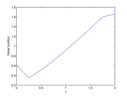
Figure 1: Approximate value function with $h_{1}=0.25$ and $h_{2}=0.001$ for fixed expectation

The value function is plotted in Figure 1, the corresponding control in Figure 2, and the efficient frontier in Figure 3.

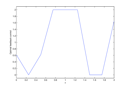
Figure 2: Optimal feedback control with $h_{1}=0.25$ and $h_{2}=0.001$ for fixed expectation

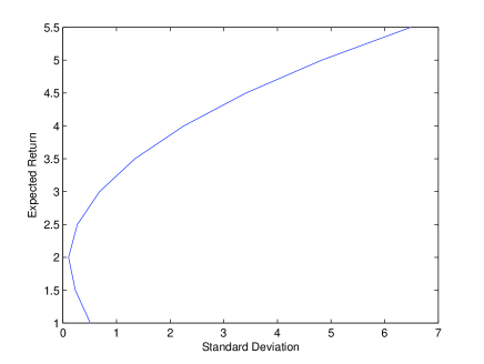
Figure 3: Efficient frontier $h_{1}=0.25$ and $h_{2}=0.001$ when using simplex method to find out the optimal $\lambda$

6.2 Further Remarks

This paper developed a numerical approach for a controlled switching diffusion system with a hidden Markov chain. Using Markov chain approximation techniques combined with the Wonham filtering, a numerical scheme was developed. In contrast to the existing work in the literature, we used Markov chain approximation for the diffusion component and used a direct discretization for the Wonham filter. Our on-going effort will be directed to use the approach developed in this work to treat certain networked systems that involve platoon controls with wireless communications.

References

- [1]
- [2]
- [3] S. Chen, X. Li, and X.Y. Zhou, stochastic linar quadratic regulators with indefinite control weight costs, SIAM J. Control Optim., 36 (1998), 1685–1702.
- [4] F. Dufour and P. Bertrand, The filtering problem for continuous time linear systems with Markovian switching coefficients, Syst. Control Lett., 23 (1994), 453–461.
- [5] D. Duffie and H. Richardson, Mean-variance hedging in continuous time, Ann. Appl. Probab., 1 (1991), 1–15.
- [6] W.H. Fleming and M. Nisio, On stochastic relaxed control for partially observed diffusions, Nagoya Math. J., 93 (1984), 71–108.
- [7] H.J. Kushner, Numerical methods for stochastic control problems in continuous time, SIAM J. Control Optim., 28 (1990), 999–1048.
- [8] H.J. Kushner, Consistency issues for numerical methods for variance control with applications to optimization in finance, IEEE. Trans. Automat. Control, 44 (2000), 2283–2296.
- [9] H.J. Kushner and P. Dupuis, Numerical Methods for Stochastic Control Problems in Continuous Time, Springer, New York, 2001.
- [10] D. Li and W.L. Ng, Optimal dynamic portfolio selection: Multi-period mean-variance formulation, Math. Finance., 10 (2000), 387–406.
- [11] H. Markowitz, Portfolio selection, J. Finance., 7 (1952), 77–91.
- [12] P.A. Samuelson, Lifetime portfolio selection by dynamic stochastic programming, Rev. Econ. Statist., 51 (1969), 239–246.
- [13] S.R. Pliska, Introduction to Mathematical Finance, Basil Blackwell, Malden, UK, 1997.
- [14] M. Schweizer, Approximation pricing and the variance optimal martingale measure, Ann. Probab., 24 (1996), 206–236.
- [15] Q.S. Song, G. Yin, and Z. Zhang, Numerical method for controlled regime-switching diffusions and regime-switching jump diffusions, Automatica, 42 (2006), 1147–1157.
- [16] W.M. Wonham, Some applications of stochastic differential equations to optimal nonlinear filtering, SIAM J. Control, 2 (1965), 347–369.
- [17] Z. Yang, G. Yin, L,Y, Wang, and H. Zhang, Near-Optimal mean-variance controls under two-time-scale formulations and applications, Stochastics, 85 (2013), 723–741.
- [18] D. Yao, Q. Zhang, X.Y. Zhou, A regime switching model for European options, in Stochastic Process, Optimization, and Control Theory, H. Yan, G. Yin and Q. Zhang Eds., 281–300, Springer, 2006.
- [19] G. Yin and Q. Zhang, Discrete-Time Markov chains: Two-time-scale methods and application, Springer, New York, 2005.
- [20] G. Yin and X.Y. Zhou, Markowitz mean-variance portfolio selection with regime switching: from discrete-time models to their continuous-time limits, IEEE Trans. Automatic Control., 49 (2004), 349–360.
- [21] G. Yin and C. Zhu, Hybrid Switching Diffusions. New York: Springer, 2010.
- [22] J. Yong and X.Y. Zhou, Stochastic controls: Hamiltonian Sytems and HJB Equations. New York: Springer, 1999.
- [23] L. Yu, Q. Zhang and G. Yin, Asset allocation for regime switching market models under partial observation, to appear in Dynamic Systems and Applications.
- [24] Q. Zhang, Stock trading: an optional selling rule, SIAM J.Control Optim., 40 (2001), 64–87.
- [25] X.Y. Zhou and D. Li, Continuous time mean variance portfolio selection: A stochastic LQ Framework, Appl Math Optim, 42 (2000), 19–33.
- [26] X.Y. Zhou and G. Yin, Markowitz mean-variance portfolio selection with regime switching: A continuous time model, SIAM J.Control Optim., 42 (2003), 1466–1482.