Thermo-electromechanical effects in relaxed shape graphene and bandstructures of graphene quantum dots

Abstract

We investigate the in-plane oscillations of the relaxed shape graphene due to externally applied tensile edge stress along both the armchair and zigzag directions. We show that the total elastic energy density is enhanced with temperature for the case of applied tensile edge stress along the zigzag direction. Thermo-electromechanical effects are treated via pseudomorphic vector potentials to analyze the influence of these coupled effects on the bandstructures of bilayer graphene quantum dots (QDs). We report that the level crossing between ground and first excited states in the localized edge states can be achieved with the accessible values of temperature. In particular, the level crossing point extends to higher temperatures with decreasing values of externally applied tensile edge stress along the armchair direction. This kind of level crossings is absent in the states formed at the center of the graphene sheet due to the presence of three fold symmetry.

I Introduction

Miniaturization is one of the requirements to make electronic devices smaller and smaller. To fulfill this requirement, graphene based electronic devices might provide a breakthrough alternative for the current state-of-the-art semiconductor industry. Graphene is a promising material to build electronic devices because of its unusual properties due to the Dirac-like spectrum of the charge carriers. Novoselov et al. (2004, 2005) In addition, researchers around the world seek to make next generation electronic devices from graphene because the material possesses high charge mobility. There is an opportunity to control electronic properties of graphene-based structures by several different techniques such as gate controlled electric fields, magnetic fields, and to engineer the electromechanical properties via pseudomorphic gauge fields. Castro Neto et al. (2009); Shenoy et al. (2008); Choi et al. (2010); Maksym and Aoki (2013); Bao et al. (2012); Yan et al. (2012); Cadelano et al. (2009); Cadelano and Colombo (2012); Bao et al. (2009) Recently, spin echo phenomena, followed by strong beating patterns due to rapid oscillations of quantum states along a graphene ribbon, have been investigated for realization of quantum memory at optical states in the far-infrared region for quantum information processing. Prabhakar et al. (2013); Belonenko et al. (2012)

Graphene sheets designed to make next generation electronic devices consist of surfaces that are not perfectly flat. The surfaces exhibit intrinsic microscopic roughening, the surface normal varies by several degrees and the out-of-plane deformations reach to the nanometer scale. Gass et al. (2008); Shenoy et al. (2008); Meyer et al. (2007); Bonilla and Carpio (2012); Guinea et al. (2010) Out-of-plane displacements without a preferred direction induce ripples in the graphene sheet, Gibertini et al. (2010); Wang and Upmanyu (2012); Bonilla and Carpio (2012); Carpio and Bonilla (2008); San-Jose et al. (2011) while in-plane displacements induced by applying suitable tensile edge stress along the armchair and zigzag directions lead to the relaxed shape graphene. Gass et al. (2008); Shenoy et al. (2008) In experiments with graphene suspended on substrate trenches, there appear much longer and taller waves (close to a micron scale) directed parallel to the applied stress. Gass et al. (2008); Shenoy et al. (2008); Cerda and Mahadevan (2003) These long wrinkles are mechanically induced and we know that theoretically it is possible to corrugate an elastic membrane at absolute zero temperature. The mechanical deformation of a free standing graphene sheet can be understood by applying suitable edge stress along the armchair and zigzag directions. The tensile forces, that can be applied on the graphene sheet with a compressed elastic string, are schematically shown in Fig. 1. In this paper, we show that intrinsic edge stresses can have a significant influence on the morphology of graphene sheets and substantially modify the bandstructures of graphene quantum dots. We present a model that couples the Navier equations, accounting for thermo-electromechanical effects, to the electronic properties of graphene quantum dots. Zakharchenko et al. (2009) Here we show that the amplitude of the induced waves due to applied tensile edge stress along the armchair and zigzag directions increases with temperature and provides the level crossing in the localized edge states. This kind of level crossings is absent for the states formed at the center of the graphene sheet due to the presence of three fold symmetry induced by pseudomorphic strain tensor.

II Theoretical Model

The total thermoelastic energy density associated to the strain for the two-dimensional graphene sheet can be written as Landau and Lifshitz (1970a); Carpio and Bonilla (2008); Cadelano and Colombo (2012)

$$U_{s}=\frac{1}{2}C_{iklm}\varepsilon_{ik}\varepsilon_{lm}-\beta_{ik}\Theta(x,y)\varepsilon_{ik}\delta_{ik},~{}~{}~{}~{}$$ (1)

where $C_{iklm}$ is a tensor of rank four (the elastic modulus tensor), $\varepsilon_{ik}$ (or $\varepsilon_{lm}$) is the strain tensor and $\beta_{{}_{ik}}$ are the stress temperature coefficients. Also, $\Theta(x,y)$ is the distribution of temperature in the graphene sheet that can be found by solving Laplace’s equation $\partial_{i}q_{i}=0$, where $q_{i}=-\alpha_{{}_{ii}}\partial_{x_{i}}\Theta$ with $\alpha_{{}_{ii}}$ being the heat induction coefficients of graphene. Thus we write the Laplace’s equation as

$$\alpha_{{}_{11}}\partial_{x}^{2}\Theta+\alpha_{{}_{22}}\partial_{y}^{2}\Theta=0.$$ (2)

We suppose that the graphene sheet at the boundary 4 (see Fig. 1) is connected to the heat bath of temperature $T(x)$ and all other three boundaries 1,2,3 are fixed at zero temperature. Thus, the exact solution of Laplace’s equation can be written as

$$\Theta\left(x,y\right)=\sum_{m=1}^{\infty}B_{m}\sinh\left(\frac{m\pi y}{L\sqrt{k_{e}}}\right)\sin\left(\frac{m\pi}{L}x\right),$$ (3)

where the constant $B_{m}$ relates to the temperature of the thermal bath $T(x)$ as:

$$T(x)=\sum_{m=1}^{\infty}B_{m}\sinh\left(\frac{m\pi w}{L\sqrt{k_{e}}}\right)\sin\left(\frac{m\pi}{L}x\right).$$ (4)

Here $k_{e}=\alpha_{{}_{22}}/\alpha_{{}_{11}}$, m is an integer, $L$ is the length and $w$ is the width of the graphene sheet. The arbitrary constant $B_{m}$ can be found by performing Fourier’s transform of (4):

$$B_{m}=\frac{2}{L\sinh\left(m\pi w/L\sqrt{(}k_{e})\right)}\int_{0}^{L}T(x)\sin\left(\frac{m\pi x}{L}\right)dx.$$ (5)

In (1), the strain tensor components can be written as

$$\varepsilon_{ik}=\frac{1}{2}\left(\partial_{x_{k}}u_{i}+\partial_{x_{i}}u_{k}+\partial_{x_{k}}h\partial_{x_{i}}h\right),$$ (6)

where $u_{i}$ and $h$ are in-plane and out-of-plane displacements, respectively. de Juan et al. (2013); Carpio and Bonilla (2008) It is believed that the ripples in graphene have two different types of sources (see Figs. 1 and 3 of Ref. Thompson-Flagg et al., 2009). Both types of ripple waves are considered to be the sinusoidal function of position whose amplitude lies normal to the plane of two-dimensional graphene sheet. The origin of first type ripples results in the relaxed shape graphene (i.e., the displacement vector relaxed to the equilibrium position where the total elastic energy density is minimized) due to externally applied in-plane (along x and y-directions only) tensile edge stress. Shenoy et al. (2008) Such kind of ripples that can be seen in the form of relaxed shape graphene occurs in a fashion similar to leaves or torn plastic Sharon et al. (2002) where buckling mechanism displaces only the carbon atoms near the edge of the graphene sheet. Thompson-Flagg et al. (2009); Shenoy et al. (2008) While the origin of second type ripples results in the height fluctuations through out the graphene sheet due to adsorbed hydroxide molecules sitting on random sites of hexagon graphene molecules in a two-dimensional graphene sheet. Echtermeyer et al. ; Fasolino et al. (2007); Moser et al. (2008) In this paper, we only consider the ripple waves induced by buckling mechanisms ($i.e.,h=0$) by applying tensile edge stress along the armchair and zigzag directions. Shenoy et al. (2008); not Hence the strain tensor components for graphene in 2D displacement vector $\mathbf{u}(x,y)=(u_{x},u_{y})$ can be written as

$$\varepsilon_{xx}=\partial_{x}u_{x},~{}\varepsilon_{yy}=\partial_{y}u_{y},~{}\varepsilon_{xy}=\frac{1}{2}\left(\partial_{y}u_{x}+\partial_{x}u_{y}\right).$$ (7)

The stress tensor components $\sigma_{ik}=\partial U_{s}/\partial\varepsilon_{ik}$ for graphene can be written as Zhou and Huang (2008)

$$\sigma_{xx}=C_{11}\varepsilon_{xx}+C_{12}\varepsilon_{yy}-\beta_{11}\Theta,$$ (8)

$$\sigma_{yy}=C_{12}\varepsilon_{xx}+C_{22}\varepsilon_{yy}-\beta_{22}\Theta,$$ (9)

$$\sigma_{xy}=2C_{66}\varepsilon_{xy}.$$ (10)

In the continuum limit, elastic deformations of graphene sheets are described by the Navier equations $\partial_{j}\sigma_{ik}=0$. Hence, the coupled Navier-type equations of thermoelasticity for graphene can be written as

$$\left(C_{11}\partial^{2}_{x}+C_{66}\partial^{2}_{y}\right)u_{x}+\left(C_{12}+C_{66}\right)\partial_{x}\partial_{y}u_{y}=\beta_{11}\Theta_{x},~{}~{}~{}~{}~{}$$ (11)

$$\left(C_{66}\partial^{2}_{x}+C_{22}\partial^{2}_{y}\right)u_{y}+\left(C_{12}+C_{66}\right)\partial_{x}\partial_{y}u_{x}=\beta_{22}\Theta_{y},~{}~{}~{}~{}~{}$$ (12)

where

$$\Theta_{x}=\sum_{m=1}^{\infty}\frac{m\pi B_{m}}{L}\sinh\left(\frac{m\pi y}{L\sqrt{k_{e}}}\right)\cos\left(\frac{m\pi}{L}x\right),$$ (13)

$$\Theta_{y}=\sum_{m=1}^{\infty}\frac{m\pi B_{m}}{L\sqrt{(}k_{e})}\cosh\left(\frac{m\pi y}{L\sqrt{k_{e}}}\right)\sin\left(-\frac{m\pi}{L}x\right).$$ (14)

Now we apply the compressive tensile edge stresses through the boundaries of the graphene sheet (see Fig. 1) along the lateral directions and seek to establish the relationship between the waves generated due to applied tensile edge stresses and the in-plane displacement vector. More precisely, the mechanical deformation along the lateral direction of a graphene sheet can be understood by considering the effect of externally applied tensile edge stresses along the lateral direction in the form of compressed elastic string between which the 2-dimensional free standing graphene sheet is clamped. Landau and Lifshitz (1970b); Zhou and Huang (2008); Cadelano et al. (2009) It is natural to expect that the longitudinal waves, generated by compressed elastic forces, travel along the direction of applied tensile edge stresses. Hence we might think the sinusoidal function in the deformation of in-plane displacement vectors that correlate the geometric features of the longitudinal waves generated in the graphene sheet due to compressed elastic tensile edge stresses which finally turn the flat surface of the graphene sheet into the relaxed shape graphene in the form of torn plastic. Thus we assume the functional form of $\mathbf{u}\left(x,y\right)$ at the boundary $2$ of armchair as:

$$u(x,0)=u_{x}=A\sin\left(kx\right),$$ (15)

where $A$ is the amplitude and $k=2\pi/\lambda$ with $\lambda$ being the wavelength while the total edge energy per unit length becomes Shenoy et al. (2008)

$$U_{e}=\frac{1}{2}\tau_{e}\left(\frac{\partial u\left(x,0\right)}{\partial x}\right)^{2}+\frac{1}{8}E_{e}\left(\frac{\partial u\left(x,0\right)}{\partial x}\right)^{4},$$ (16)

where $\tau_{e}$ and $E_{e}$ denote the edge stress and the elastic modulus of the edge along the armchair direction of the graphene sheet. Thus, we write the total edge energy $U_{t}=\int_{0}^{L}U_{e}dx$ and find the optimum amplitude of the waves along the armchair direction by utilizing the condition $\partial U_{t}/\partial A=0$ to be:

$$A=\sqrt{\frac{2\tau_{e}\left(2kL+\sin\left(2kL\right)\right)}{E_{e}k^{2}\left[12kL+8\sin\left(2kL\right)+\sin\left(4kL\right)\right]}}.$$ (17)

By considering $L=1.5~{}\mathrm{\mu m}$, $\tau_{e}=4~{}\mathrm{eV/nm}$, $E_{e}=1000~{}\mathrm{eV/nm}$ and $\lambda=0.1$ to $1.5~{}\mathrm{\mu m}$, the amplitude ($\mathrm{A}$) of the waves varies from $0.6~{}\mathrm{nm}$ to $8.7~{}\mathrm{nm}$. This amplitude decreases exponentially as it moves into the graphene sheet along y-direction. Thus we assume $u\left(x,y\right)=A\sin\left(kx\right)\exp{\left(-y/\ell\right)}$, where $\ell$ is the penetration depth of the ripple waves and write the total elastic energy of the graphene sheet as $\tilde{U}=U_{t}+\int^{L}_{x=0}\int^{\infty}_{y=0}U_{s}dxdy$. By considering $\partial\tilde{U}/\partial A=0$, we found the functional form of the amplitude as

$$2A\Gamma_{1}+4A^{3}\Gamma_{2}-\Gamma_{3}+\Gamma_{4}=0,$$ (18)

where

$$\Gamma_{1}=\frac{k}{16}\left(2\tau_{e}+c_{11}\ell+c_{66}\ell\right)\left\{\sin\left(2kL\right)+2kL\right\}-\frac{1}{16k\ell}\left(c_{22}+c_{66}\right)\left\{\sin\left(2kL\right)-2kL\right\}-\frac{1}{4}\left(c_{12}+c_{66}\right)\sin^{2}\left(kL\right),$$ (19)

$$\Gamma_{2}=\frac{E_{e}k^{3}}{32}\left\{12kL+8\sin\left(2kL\right)+\sin\left(4kL\right)\right\},$$ (20)

$$\Gamma_{3}=\beta_{11}k\sum_{m=1}^{\infty}\frac{B_{m}}{2}\left\{\frac{\cos\left(m\pi+kL\right)}{m\pi+kL}+\frac{\cos\left(m\pi-kL\right)}{m\pi+kL}-\frac{2m\pi}{m^{2}\pi^{2}-k^{2}L^{2}}\right\}\frac{m\pi L^{2}\ell^{2}\sqrt{k_{e}}}{m^{2}\pi^{2}\ell^{2}-L^{2}\sqrt{k_{e}}},$$ (21)

$$\Gamma_{4}=\beta_{11}\sum_{m=1}^{\infty}\frac{B_{m}}{2}\left\{\frac{\sin\left(m\pi+kL\right)}{m\pi+kL}+\frac{\sin\left(m\pi-kL\right)}{m\pi+kL}\right\}\frac{m\pi L^{2}\ell\sqrt{k_{e}}}{m^{2}\pi^{2}\ell^{2}-L^{2}\sqrt{k_{e}}}.$$ (22)

At absolute zero temperature (i.e., $\Gamma_{3}=\Gamma_{4}=0$), the amplitude of the ripple waves obtained from Eq. (18) resembles the expression presented in Ref. Shenoy et al., 2008. Similar type of expression (18) can also be obtained for the optimum amplitude of the longitudinal waves along the zigzag direction by considering non-vanishing $u\left(0,y\right)=u_{y}=A\sin{\left(ky\right)}$ in (15) and replacing $L$ by $w$ in (17).

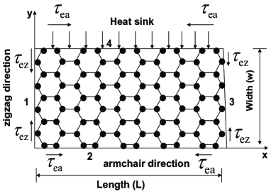
Figure 1: Tensile stress is applied along armchair and zigzag directions that induce the oscillation in strain tensor in graphene sheet. The boundary 4 is connected to the heat bath to investigate the influence of temperature on the strain tensor as well as on the bandstructures of graphene.

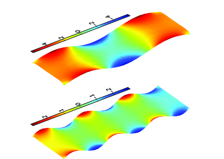
Figure 2: Relaxed shape of graphene due to applied tensile stress along armchair direction for $\lambda=1~{}\mathrm{\mu m}$ (upper panel) and $\lambda=0.5~{}\mathrm{\mu m}$ (lower panel). Here we chose $T(x)=T_{0}=75~{}\mathrm{K}$, $\tau_{e}=4~{}\mathrm{eV/nm}$, $E_{e}=1000~{}\mathrm{eV/nm}$ and the dimension of the graphene sheet is taken to be $L\times w=1.5\times 0.5~{}\mathrm{\mu m^{2}}$. The longer and shorter sides are considered as the armchair and zigzag edges respectively. The variation in the amplitude of the ripple waves, expressed in nanometer, is shown in the color bar.

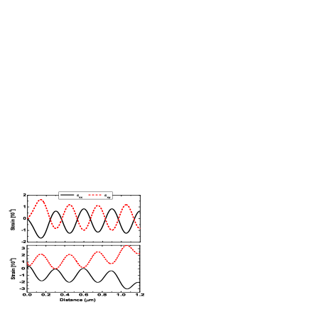
Figure 3: Oscillations in strain tensor due to applied tensile stress along the armchair direction at $y=w/2$ and temperature $T_{0}=0~{}\mathrm{K}$ (upper panel) and $T_{0}=300~{}\mathrm{K}$ (lower panel). The parameters are chosen to be the same as in Fig. 2 but wavelength $\lambda=300~{}\mathrm{nm}$.

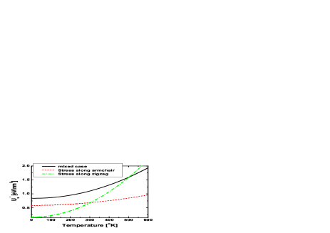
Figure 4: Free elastic energy density, $U_{s}^{\prime}=1/\tilde{A}\left(\int_{\Omega}U_{s}dxdy\right)$ with $\tilde{A}=L\times w$ and $\Omega$ being the computational domain. For mixed case, we have applied the tensile edge stress along both the armchair and zigzag direction. The parameters are chosen to be the same as in Fig. 2.

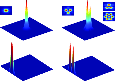
Figure 5: Demonstration of squared wavefunctions, $|\Psi|^{2}$ formed by lateral confined potential $U(x,y)$ (see Eq. 23) in $L\times w=400\times 400~{}\mathrm{nm^{2}}$ graphene sheet. Upper panel shows the states formed at the center of the graphene sheet and lower panel shows the edge states formed at the zigzag boundary 1 (see Fig. 1). Note that in the upper panel, unusual first excited state wavefunction can be seen due to the presence of three fold symmetry in graphene. For eigenvalues see Fig. 6. For electromechanical parts, we chose $\tau_{e}=45\mathrm{eV/nm}$, $E_{e}=1000\mathrm{eV/nm}$ and $T_{0}=5\mathrm{K}$ that mimic the experimentally reported values in Ref. Lee et al., 2008. For bandstructure calculations, we chose $U_{0}=0.2\mathrm{eV}$, $\lambda_{1}=\lambda_{2}=200\mathrm{nm}$ and dimensionless parameter $\xi=1.97$.

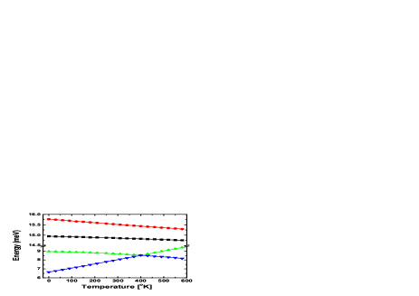
Figure 6: Ground and first excited states eigenenergies formed at the center of the graphene sheet (diamonds and circles) and at the edge of boundary 1 (triangles pointing up and triangles pointing down) vs temperature for the case $\tau_{e}=45~{}\mathrm{eV/nm}$ along the armchair direction. It can be seen that the level crossing between ground and first excited states edge energy occurs at $T=400~{}K$. The parameters are chosen to be the same as in Fig. 5.

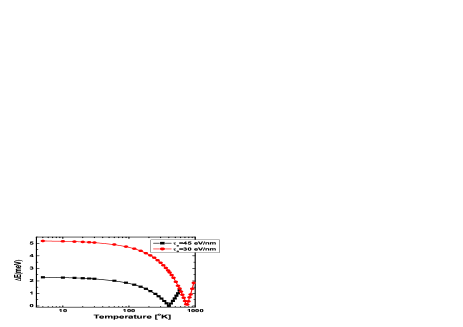
Figure 7: Edge energy difference $\Delta E=E_{1}-E_{2}$ for the states at boundary 1 vs temperature. We can see that the level crossing point extends to larger temperatures with the decreasing values of the externally applied tensile edge stress along the armchair direction.

Table 1: The material constants for graphene used in our calculations are taken from Refs. Carpio and Bonilla, 2008; Shenoy et al., 2008; Shen et al., 2010; Yoon et al., 2011; Bao et al., 2009.

Parameters
$C_{11}$[N/m]=$C_{22}$	359.4
$C_{12}$[N/m]	41
$C_{66}$[N/m]	159.2
$\alpha_{{}_{11}}[10^{-6}/\mathrm{K}]$	-7
$\alpha_{{}_{22}}[10^{-6}/\mathrm{K}]$	-7
$\beta_{11}[10^{-3}\mathrm{N}/\left(\mathrm{m}\cdot\mathrm{K}\right)]$a	-2.8
$\beta_{22}[10^{-3}\mathrm{N}/\left(\mathrm{m}\cdot\mathrm{K}\right)]$a	-2.8

^aThe numerical values of the thermal coefficients $\beta_{11}$ and $\beta_{22}$ are obtained from expressions $\beta_{11}=C_{11}\alpha_{{}_{11}}+C_{12}\alpha_{{}_{22}}$ and $\beta_{22}=C_{12}\alpha_{{}_{11}}+C_{22}\alpha_{{}_{22}}$.

Now we turn to the analysis of the influence of strain on the electronic properties of graphene QDs formed in the graphene sheet with the application of parabolic gate potential. In the continuum limit, by expanding the momentum close to the $K$ point in the Brillouin zone, the Hamiltonian reads $H=\sum_{k}\Psi_{k}^{\dagger}\cdot H_{k}\cdot\Psi_{k}$. Here $H_{k}$ is written as Maksym and Aoki (2013); Krueckl and Richter (2012); Castro Neto et al. (2009)

$$H_{k}=\left(\begin{array}[]{cccc}-U(x,y)&v{{}_{{}_{F}}}P_{+}&0&\frac{3\gamma_{3}aP_{-}}{\hbar}\\ v{{}_{{}_{F}}}P_{-}&-U(x,y)&\gamma_{1}&0\\ 0&\gamma_{1}&U(x,y)&-v{{}_{{}_{F}}}P_{-}\\ \frac{3\gamma_{3}aP_{+}}{\hbar}&0&-v{{}_{{}_{F}}}P_{+}&U(x,y)\end{array}\right),$$ (23)

where $P_{\pm}=P_{x}\pm iP_{y}$ and $P=p-\hbar A$ with $p=-i\hbar\partial_{x}$ being the canonical momentum operator and $\textbf{A}=\beta\left(\varepsilon_{xx}-\varepsilon_{yy},\varepsilon_{xy}\right)/a$ is the vector potential induced by pseudomorphic strain tensor. Guinea et al. (2008); de Juan et al. (2013) Also, $a$ is the lattice constant, $v_{F}=10^{6}\mathrm{m/s}$ is the Fermi velocity, $\gamma_{3}=0.3\mathrm{eV}$ corresponds to the interaction energy between two neighboring atoms A and B placed one under the other (see Ref. Castro Neto et al., 2009) and $\beta=-\partial\ln t/\partial\ln a\approx 2$ with $t$ being the nearest neighbor hoping parameters. We assume a confining potential $U(x,y)=U_{x}+U_{y}$ that decays exponentially away from the edges into the bulk with a penetration depths $\lambda_{1}$ or $\lambda_{2}$. Here we write $U(x)$ and $U(y)$ as: Castro Neto et al. (2009); Maksym and Aoki (2013)

$$U(x)=U_{0}\left\{\exp{\left(\frac{-2x+L}{2\lambda_{1}}\right)}+\exp{\left(\frac{2x-L}{2\lambda_{1}}\right)}-\xi\right\},~{}~{}~{}~{}~{}$$ (24)

$$U(y)=U_{0}\left\{\exp{\left(\frac{-2y+w}{2\lambda_{2}}\right)}+\exp{\left(\frac{2y+w}{2\lambda_{2}}\right)}-\xi\right\},~{}~{}~{}~{}~{}$$ (25)

where $\lambda_{1}=L/2$, $\lambda_{2}=w/2$ and $\xi$ is a dimensionless constant. We can vary $\xi$ to vary the band gap of graphene induced by gate potential.

III Results and Discussions

The schematic diagram of the two-dimensional graphene sheet in computational domain is shown in Fig. 1. We have applied the tensile edge stress along both the armchair and zigzag directions to create oscillations in strain tensor of the graphene sheet. We have used the multiphysics simulation and solved the Navier’s equations (11) and (12) via Finite Element Method to investigate the influence of thermo-electromechanical effects on the relaxed shape of graphene. For the waves along the armchair direction, we have used the Neumann boundary conditions at sides 1, 3 and employed Eq. (15) at sides 2,4 and vice versa for the zigzag direction. All reported results (Figs. 2-4) have been obtained for a $1.5\times 0.5~{}\mathrm{\mu m^{2}}$ graphene sheet that mimics the geometry of experimentally studied structures in Refs. Bao et al., 2009. All parameters for our simulations have been taken from Table 1. For bandstructure calculations (Figs. 5-7), we have chosen a $400\times 400~{}\mathrm{nm^{2}}$ graphene sheet.

Fig. 2 shows the relaxed shape of graphene under applied tensile stress along the armchair direction. The variation in the amplitude of ripple waves, expressed in nanometer, is shown in the color bar (see Eq. 17). As can be seen in the color bar, the amplitude of the ripple waves in the relaxed shape graphene is enhanced with the increasing values of the wavelength which is also supported analytically by Eq. (17). In Fig. 3, we investigate the influence of temperature on the strain tensor under an applied tensile edge stress along the armchair direction. Again, the oscillations in the strain tensor occur due to the applied tensile stress along the armchair direction that induces longitudinal waves and propagate along the armchair direction. We note that the increasing temperature from $0~{}\mathrm{K}$ (upper panel) to room temperature (lower panel) enhances the amplitude of the waves that eventually increase the magnetic field of the pseudomorphic vector potentials and allow us to investigate its influence in the bandstructure calculation of graphene at Dirac points (for details, see Figs. 6 and 7). In Fig. 4, we investigate the total elastic energy density vs temperature. Even though the optimum values of the amplitudes of waves along the armchair and zigzag directions are exactly the same, the variation in the total free elastic energy density is enhanced for the case of applied tensile edge stress along the zigzag direction (dashed-dotted line). This occurs because the graphene sheet along the boundary 4 is connected to the heat reservoir that enhances the free elastic energy of the waves traveling along the zigzag direction.

Another important result of the paper is the study of the influence of thermomechanics on the bandstructure of bilayer graphene QDs via pseudomorphic vector potentials. In Fig. 5, we have plotted several states wavefunctions of the graphene QDs. It can be seen that in addition to the localized states formed at the center of the graphene sheet, edge states are also present at the zigzag boundary. The localized edge states at the zigzag boundary can be seen due to the fact that the pseudomorphic vector potential originating from the thermo-electromechanical effects generates a large magnetic field applied perpendicular to the two-dimensional graphene sheet. For example, considering $\mathbf{B}=\nabla\times\mathbf{A}$, we find $B_{z}=\left(2\pi\beta\varphi_{0}/a\right)\left\{\partial_{x}\varepsilon_{xy}-\partial_{y}\left(\varepsilon_{xx}-\varepsilon_{yy}\right)\right\}$, where $\varphi_{0}=\hbar/e$. Further, by assuming sinusoidal functions of strain tensor (see Fig. 3) generated by applying tensile edge stress along the armchair direction, for example: $\varepsilon_{xx}=-\varepsilon_{xy}=\varepsilon_{0}\sin\left(kx\right)$ and $\varepsilon_{yy}=0$, where $\varepsilon_{0}$ is the amplitude of the strain tensor, we find $B_{z}=-B_{0}\cos\left(kx\right)$, where $B_{0}=2\pi\varepsilon_{0}\beta k\hbar/ae$. By considering $\lambda=300\mathrm{nm}$ and $\varepsilon_{0}=10^{-3}$ (see Fig. 3 (upper panel)), we estimate $B_{0}\approx 1.2~{}\mathrm{tesla}$. Hence such a large magnetic field along z-direction originating from electromechanical effects induces a persistent current that flows toward the edge of the graphene. As a result, a positive (negative) dispersion in the electron (hole) like states is induced at the zigzag edge (also see Fig.4 of Ref. Castro Neto et al., 2006) and the localized electron-hole states wavefunction drift towards and over the edge of graphene sheet. Wen (1992); Castro Neto et al. (2006); Vikstroöm (2014) Hence the wavefunctions that are pressed against the edge finally turn into the localized edge current carrying states. Castro Neto et al. (2006); Zarenia et al. (2011); Vikstroöm (2014); Wen (1992) Similar kind of localized edge states are also shown in Fig. 2(d) of Ref. Castro Neto et al., 2006. Furthermore, by utilizing tight binding and continuum model, the authors in Ref. Zarenia et al., 2011 have shown that the tunneling effect at the interface between the internal and external regions of the dots can be avoided and consequently the charge carriers are confined at the zigzag edge (for example see Eq. (11) and left panel of Fig. 6 of Ref. Zarenia et al., 2011). Such localized edge states, shown in the lower panel of Fig. 5 in this paper, are highly sensitive to the applied tensile edge stress along the armchair and zigzag directions. We observe three fold symmetry in the first excited state wavefunction (see inset plot of Fig. 5) of graphene that is in agreement to the experimentally reported results (see Fig.(4) of Ref. Klimov et al., 2012) and as well as previously reported theoretical results (see Ref. Moldovan et al., 2013). In Fig. 6, we find the level crossing at $T=400K$ due to the fact that the edge energy difference between the ground and first excited states decreases with increasing temperature. This level crossing point extends to higher temperatures with decreasing values of tensile edge stress (see Fig. 7). We have analyzed why the level crossing point can be seen on the edge states, but cannot be seen on the localized states formed at the center of the graphene sheet. The reason is that the graphene sheet on boundary 4 is connected to the heat reservoir. Hence, the energy difference between the ground and first excited states decreases with increasing temperature. As a result, we find the level crossing in the edge states to be at the zigzag boundary with the accessible values of temperatures. The energy difference between the ground and first excited states formed at the center of the graphene sheet also decreases with increasing temperature (see Fig. 6). However, such energy states do not meet each other with any practically applicable values of the temperature due to absence of two fold symmetry in graphene. In fact, the induced pseudomorphic fields by the strain tensor affect the graphene charge carriers and produce a three fold symmetry in the wavefunction of two-dimensional graphene sheet (see inset plot of 5). The symmetry of the pseudomorphic fields is determined by the corresponding symmetry of the strain field. For example, a uniform pseudomorphic field requires a special strain field distorted with three fold symmetry. Klimov et al. (2012); Guinea et al. (2010)

IV Conclusion

To conclude, we have developed a model which allows us to investigate the influence of temperature on the relaxed shape of the graphene sheet as well as in the QDs that are formed in the two-dimensional graphene sheet with the application of gate potentials. We have shown that the variation in the total free elastic energy density is enhanced with temperature for the case of applied tensile edge stress along the zigzag direction. We have treated the strain, induced by an applied tensile edge stress along the armchair and zigzag directions, as a pseudomorphic vector potential and shown that the level crossing point between the ground and first excited edge states at the zigzag boundary extends to higher temperatures with decreasing values of the tensile edge stress. Such kind of level crossing is absent in the states formed at the center of the graphene sheet due to the presence of three fold symmetry.