Auxiliary field Monte-Carlo simulation
of strong coupling lattice QCD for QCD phase diagram

Abstract

We study the QCD phase diagram in the strong coupling limit with fluctuation effects by using the auxiliary field Monte-Carlo method. We apply the chiral angle fixing technique in order to obtain finite chiral condensate in the chiral limit in finite volume. The behavior of order parameters suggests that chiral phase transition is the second order or crossover at low chemical potential and the first order at high chemical potential. Compared with the mean field results, the hadronic phase is suppressed at low chemical potential, and is extended at high chemical potential as already suggested in the monomer-dimer-polymer simulations. We find that the sign problem originating from the bosonization procedure is weakened by the phase cancellation mechanism; a complex phase from one site tends to be canceled by the nearest neighbor site phase as long as low momentum auxiliary field contributions dominate.

D30, B64, D34,

1 Introduction

Quantum Chromodynamics (QCD) phase diagram is attracting much attention in recent years. At high temperature ($T$), there is a transition from quark-gluon plasma (QGP) to hadronic matter via the crossover transition, which was realized in the early universe and is now extensively studied in high-energy heavy-ion collision experiments at RHIC and LHC. At high quark chemical potential ($\mu$), we also expect the transition from baryonic to quark matter, which may be realized in cold dense matter such as the neutron star core. Provided that the high density transition is the first order, the QCD critical point (CP) should exist as the end point of the first order phase boundary. Large fluctuations of the order parameters around CP may be observed in the beam energy scan program at RHIC.

The Monte-Carlo simulation of the lattice QCD (MC-LQCD) is one of the first principle non-perturbative methods to investigate the phase transition. We can obtain various properties of QCD: hadron masses and interactions, color confinement, chiral and deconfinement transitions, equation of state, and so on. We can apply MC-LQCD to the low $\mu$ region, but not to the high $\mu$ region because of the notorious sign problem. The fermion determinant becomes complex at finite $\mu$, then the statistical weight is reduced by the average phase factor $\left<e^{i\theta}\right>$, where $\theta$ is the complex phase of the fermion determinant. There are many attempts to avoid the sign problem such as the reweighting method Reweighting , the Taylor expansion method Taylor , the analytic continuation from imaginary chemical potential ImagMu , the canonical ensemble method Canonical , the fugacity expansion Fugacity , the histogram method Histogram , and the complex Langevin method Langevin . Many of these methods are useful for $\mu/T<1$, while it is difficult to perform the Monte-Carlo simulation in the larger $\mu$ region.

Recent studies suggest that CP may not be reachable in phase quenched simulations NoGo : In the phase quenched simulation for $N_{f}=2$, the sampling weight at finite $\mu$ is given as $|\det D(\mu)|^{2}=\det D(\mu)(\det D(\mu))^{*}=\det D(\mu)\det D(-\mu^{*})$, where $D$ represents the fermion matrix for a single flavor. The phase quenched fermion determinant for real quark chemical potential $\mu_{d}=\mu_{u}=\mu\in\mathbb{R}$ is the same as that for finite isospin and vanishing quark chemical potentials, $\mu_{d}=-\mu_{u}=\mu$. Thus the phase quenched phase diagram in the temperature-quark chemical potential $(T,\mu)$ plane would be the same as that in the temperature-isospin chemical potential $(T,\delta\mu)$ plane, as long as we can ignore the mixing of $u$ and $d$ condensates. We do not see any critical behavior in the finite $\delta\mu$ simulations outside of the pion condensed phase Finiteisospin . By comparison, the pion condensed phase appears at large $\delta\mu$, where the above correspondence does not apply. We may have CP inside the corresponding pion condensed phase. However, we now have an overlap problem; gauge configurations in the pion condensed phase would be very different from those of compressed baryonic matter which we aim to investigate. Therefore, we need to find methods other than the phase quenched simulation in order to directly sample appropriate configurations in cold dense matter for the discussion of CP and the first order phase transition.

The strong coupling lattice QCD (SC-LQCD) is one of the methods to study finite $\mu$ region based on the strong coupling expansion ($1/g^{2}$ expansion) of the lattice QCD. There are some merits to investigate the QCD phase diagram using SC-LQCD, while the strong coupling limit (SCL) is the opposite limit of the continuum limit. First, the effective action is given in terms of color singlet components, then we expect suppressed complex phases of the fermion determinant and a milder sign problem. We obtain the effective action by integrating out the spatial link variables before the fermion field integral. This point is different from the standard treatment of MC-LQCD, in which we integrate out the fermion field before the link integral. Second, we can obtain insight into the QCD phase diagram from the mean-field studies at strong coupling. The chiral transition has systematically and analytically been studied in the strong coupling expansion ($1/g^{2}$ expansion) under the mean-field approximation: the strong coupling limit (leading order, $\mathcal{O}(1/g^{0})$) SCL ; large_d ; MF-SCL ; Faldt ; BilicDeme ; Bilic ; NLOchiral ; NLOPD ; NNLO ; Jolicoeur , the next-to-leading order (NLO, $\mathcal{O}(1/g^{2})$) NLOchiral ; NLOPD ; Bilic ; BilicDeme ; Faldt ; Jolicoeur ; NNLO , and the next-to-next-to-leading order (NNLO, $\mathcal{O}(1/g^{4})$) Jolicoeur ; NNLO with staggered fermion.

It is necessary to go beyond the mean-field treatment and to include the fluctuation effects of the order parameters for quantitative studies of the finite density QCD. Monomer-dimer-polymer (MDP) simulation is one of the methods beyond the mean-field approximation. We obtain the effective action of quarks after the link integral, and evaluate the fermion integral by summing up monomer-dimer-polymer configurations KarschMutter . The phase diagram shape is modified to some extent, compared with the mean-field results on an isotropic lattice: the chiral transition temperature is reduced by 10-20 % at $\mu=0$, and the hadronic phase expands to higher $\mu$ direction by 20-30 % MDP ; PhDFromm ; MDPsign . Until now, we can perform MDP simulations only in the strong coupling limit, $1/g^{2}=0$, and the finite coupling corrections are evaluated in the reweighting method SC-Rewei . Since both finite coupling and fluctuation effects are important to discuss the QCD phase diagram, we need to develop a theoretical framework which includes both of these effects.

In this work, we study the QCD phase diagram by using an auxiliary field Monte-Carlo (AFMC) method as a tool to take account of the fluctuation effects of the auxiliary fields. AFMC is widely used in nuclear many-body problems AFMC-NP ; AFMC-NPCMP and in condensed matter physics such as ultra cold atom systems AFMC-NPCMP . In AFMC, we introduce the auxiliary fields to decompose the fermion interaction terms and carry out the Monte-Carlo integral of auxiliary fields, which is assumed to be static and constant in the mean-field approximation. We can thus include the fluctuation effects of the auxiliary fields in AFMC beyond the mean-field approximation.

Another important aspect of this paper is how to fix the chiral angle, the angle between the zero momentum scalar and pseudoscalar modes. In finite volume, symmetry of the theory is not broken spontaneously and an order parameter, in principle, vanishes. In spin systems, a root mean square order parameter is applied to obtain the appropriate order parameter MCsim1 . We here use a similar method, chiral angle fixing (CAF). The lowest momentum modes of auxiliary fields, $\sigma_{0}$ and $\pi_{0}$ in Eqs. (23) and (24), correspond to the uniform scalar and pseudoscalar modes. Then the chiral angle in each configuration is obtained by these auxiliary field modes as $\alpha=\mathrm{arctan}(\pi_{0}/\sigma_{0})$. We fix the chiral angle in each configuration by the chiral transformation so as to set $\pi_{0}=0$, and obtain quantities by using the transformed fields. We observe finite chiral condensate in the Nambu-Goldstone phase and susceptibility peak at the transition in a straightforward manner.

AFMC has several other advantages as follows. First, the chiral symmetry is manifest in the effective action. Auxiliary fields are introduced as chiral partners, $\sigma_{k}$ and $\pi_{k}$, so the chiral symmetry is obviously maintained. Second, we can directly evaluate the fluctuation effects by comparing the AFMC and mean field results. Many of the previous works on QCD phase diagram at strong coupling are carried out in the mean field analyses MF-SCL ; NLOPD ; NNLO . Next, AFMC is a natural extension of the mean field treatment, so it is straightforward to include finite coupling effects in AFMC. Finite coupling effects have been investigated in the mean field method  NLOPD ; NNLO , which can be extended to include auxiliary field fluctuations in the framework of AFMC. Finally, we can invoke various ideas to suppress the sign problem in AFMC. AFMC is a generic integral technique and utilized in many fields, where many ideas have been proposed. For example, it is promising to apply the shifted contour formulation avoidsign or the integral over Lefschetz thimbles thimble to the QCD phase diagram at strong coupling in the AFMC method.

This paper is organized as follows. In Sec. 2, we explain the formulation of AFMC in SC-LQCD. In Sec. 3, we show the numerical results on the order parameters, phase diagram, and the average phase factor. In Sec. 4, we discuss the order of the phase transition via the finite size scaling of the chiral susceptibility, and numerically confirm a source of the sign problem in AFMC . In Sec. 5, we devote ourselves to a summary and discussion.

2 Auxiliary field Monte-Carlo method

2.1 Lattice action

We here consider the lattice QCD with one species of unrooted staggered fermion for color $\mathit{SU}(N_{c})$ in the anisotropic Euclidean spacetime. Throughout this paper, we work in the lattice unit $a=1$, where $a$ is the spatial lattice spacing, and the case of color $\mathrm{SU}(N_{c}=3)$ in 3+1 dimension $(d=3)$ spacetime. Temporal and spatial lattice sizes are denoted as $N_{\tau}$ and $L$, respectively.

The partition function and action are given as,

$${\cal Z}_{\mathrm{LQCD}}= \int{\cal D}\left[\chi,{\bar{\chi}},U_{\nu}\right]e^{-S_{\mathrm{LQCD}}}\ ,$$ (1)

$$S_{\mathrm{LQCD}}= S_{F}+S_{G}\ ,$$ (2)

$$S_{F}= \frac{1}{2}\sum_{x}\left[V^{+}_{x}-V^{-}_{x}\right]+\frac{1}{2}\sum_{x}\sum_{j=1}^{d}\eta_{j,x}\left[\bar{\chi}_{x}U_{j,x}\chi_{x+\hat{j}}-\bar{\chi}_{x+\hat{j}}U^{\dagger}_{j,x}\chi_{x}\right]+m_{0}\sum_{x}M_{x}\ ,$$ (3)

$$V^{+}_{x}= \gamma e^{\mu/f(\gamma)}\bar{\chi}_{x}U_{0,x}\chi_{x+\hat{0}}\ ,$$ (4)

$$V^{-}_{x}= \gamma e^{-\mu/f(\gamma)}\bar{\chi}_{x+\hat{0}}U^{\dagger}_{0,x}\chi_{x}\ ,$$ (5)

$$M_{x}= \bar{\chi}_{x}\chi_{x}\ ,$$ (6)

$$S_{G}= \frac{2N_{c}\xi}{g_{\mathrm{\tau}}^{2}(g_{0},\xi)}\mathcal{P}_{\tau}+\frac{2N_{c}}{g_{\mathrm{s}}^{2}(g_{0},\xi)\xi}\mathcal{P}_{s}\ ,$$ (7)

$$\mathcal{P}_{i}= \sum_{P_{i}}\left[1-\displaystyle\frac{1}{2N_{c}}\mathrm{Tr}\left(U_{P_{i}}+U_{P_{i}}^{\dagger}\right)\right]\ (i=\tau,s)\ ,$$ (8)

where $\chi_{x}$, $U_{\nu,x}$, $U_{P_{\tau}}$ and $U_{P_{s}}$ represent the quark field, the link variable, and the temporal and spatial plaquettes, respectively. $\eta_{j,x}=(-1)^{x_{0}+\cdots+x_{j-1}}$ is the staggered sign factor, and $V^{\pm}_{x}$ and $M_{x}$ are mesonic composites. Quark chemical potential $\mu$ is introduced in the form of the temporal component of vector potential. The physical lattice spacing ratio is introduced as $f(\gamma)=a_{\mathrm{s}}^{\mathrm{phys}}/a_{\tau}^{\mathrm{phys}}$.

The lattice anisotropy parameters, $\gamma$ and $\xi$, are introduced as modification factors of the temporal hopping term of quarks and the temporal and spatial plaquette action terms, respectively. Temporal and spatial plaquette couplings should satisfy the hypercube symmetry condition in the isotropic limit ($\xi\to 1$), $g_{\mathrm{\tau}}(g_{0},1)=g_{\mathrm{s}}(g_{0},1)=g_{0}$. In the continuum limit ($a\to 0$ and $g_{0}\to 0$), two anisotropy parameters should correspond to the physical lattice spacing ratio, $f(\gamma)=\gamma=\xi$, when we construct lattice QCD action requiring $a_{\mathrm{s}}^{\mathrm{phys}}/a_{\tau}^{\mathrm{phys}}=\gamma$ in the continuum region, then we can define temperature as $T=f(\gamma)/N_{\tau}=\gamma/N_{\tau}$. By comparison, it seems more reasonable to define $T=\gamma^{2}/N_{\tau}$ due to quantum corrections in the strong coupling limit (SCL) as discussed based on the mean field results in Refs. Bilic ; BilicDeme ; PhDFromm . We follow this argument and adopt $f(\gamma)=\gamma^{2}$. The behavior of the chiral susceptibility suggests that this prescription is reasonable even with fluctuations as shown later in Sec. 4. We briefly summarize the mean field arguments given in Refs. Bilic ; BilicDeme ; PhDFromm in Appendix A.

In SCL, we can ignore the plaquette action terms $S_{G}$, which are proportional to $1/g^{2}$. The above lattice QCD action in the chiral limit $m_{0}\to 0$ has chiral symmetry $U(1)_{V}\times U(1)_{A}$.

2.2 Effective action

In the present formulation, we have four main steps to obtain physical observables. First, we integrate out the lattice partition function over spatial link variables in the strong-coupling limit. Second, we introduce the auxiliary fields for the mesonic composites and convert the four-Fermi interaction terms to the fermion bilinear form. Third, we perform the integral over the fermion fields and temporal link variables analytically, and obtain the effective action of the auxiliary fields. Finally, we carry out the Monte-Carlo integral over the auxiliary fields.

In the first step, we obtain the SCL effective action by integrating out spatial link variables SCL ; large_d ; MF-SCL ; Faldt ; BilicDeme ; Bilic ; NLOPD ; NNLO ; Jolicoeur ,

$$S_{\mathrm{eff}} =\frac{1}{2}\sum_{x}\left[V^{+}_{x}-V^{-}_{x}\right]-\displaystyle\frac{1}{4N_{c}}\sum_{x,j}M_{x}M_{x+\hat{j}}+m_{0}\sum_{x}M_{x}\ .$$ (9)

Here we adopt the effective action in the leading order of the $1/d$ expansion large_d , where $d$ is the spatial dimension, $d=3$.

The large dimensional expansion ($1/d$ expansion) is a scheme to truncate the interaction terms systematically. We assume that the quark fields scale as $d^{-1/4}$, then the mesonic hopping terms, second terms in Eq. (9), stay finite at large $d$. For color SU(3), spatial link integral also gives rise to spatial baryonic hopping terms which contain six quarks and sum over spatial directions, and is proportional to $\mathcal{O}(1/\sqrt{d})$. In the leading order of the $1/d$ expansion adopted here, we do not include this spatial baryonic hopping terms. One may suspect that ignoring the spatial baryonic hopping corresponds to replacing color SU(3) link integral with color U(3) and that we cannot take account of baryonic effects, but this is not true. Baryon effects arise from the temporal hopping term of quarks, first terms in Eq. (9). As we discuss later, temporal link integral is carried out exactly under the periodic and anti-periodic boundary conditions in the temporal direction for link variables and quarks, respectively. Baryon contribution naturally appears from the cubic terms of the temporal link variables, $(\bar{\chi}_{x}U_{0,x}\chi_{x+\hat{0}})^{3}$.

In the second step, we transform the four-Fermi interactions, the second terms in Eq. (9), to the fermion-bilinear form. By using the Fourier transformation in spatial coordinates $M_{x=(\mathbb{x},\tau)}=\sum_{\mathbb{k}}e^{i\mathbb{k}\cdot\mathbb{x}}M_{\mathbb{k},\tau}$, the interaction terms read

$$-\displaystyle\frac{1}{4N_{c}}\sum_{x,j}M_{x}M_{x+\hat{j}} =-\frac{L^{3}}{4N_{c}}\sum_{\mathbb{k},\tau}f(\mathbb{k})\,M_{-\mathbb{k},\tau}\,M_{\mathbb{k},\tau}\$$

$$=-\frac{L^{3}}{4N_{c}}\sum_{\mathbf{k},\tau,f(\mathbb{k})>0}f(\mathbb{k})(M_{\mathbf{k},\tau}M_{-\mathbf{k},\tau}-M_{\bar{\mathbf{k}},\tau}M_{-\bar{\mathbf{k}},\tau})\ ,$$ (10)

where $f(\mathbb{k})=\sum_{j}\cos\,k_{j}$ and $\bar{\mathbf{k}}=\mathbf{k}+(\pi,\pi,\pi)$. For later use, we divide the momentum region into the positive ($f(\mathbb{k})>0$) and negative ($f(\mathbb{k})<0$) modes. In the last line of Eq. (10), we use the relation $f(\bar{\mathbb{k}})=-f(\mathbb{k})$.

We introduce the auxiliary fields via the extended Hubbard-Stratonovich (EHS) transformation NLOPD ; NNLO . We can bosonize any kind of composite product by introducing two auxiliary fields simultaneously,

$$e^{\alpha AB} =\int\,d\varphi\,d\phi\,e^{-\alpha\left\{\left[\varphi-(A+B)/2\right]^{2}+\left[\phi-i(A-B)/2\right]^{2}\right\}+\alpha AB}$$

$$=\int\,d\varphi\,d\phi e^{-\alpha\left\{\varphi^{2}-(A+B)\varphi+\phi^{2}-i(A-B)\phi\right\}}$$

$$=\int\,d\psi\,d\psi^{*}\,e^{-\alpha\left\{\psi^{*}\psi-{A}\psi-\psi^{*}B\right\}}\ ,$$ (11)

where $\psi=\varphi+i\phi$ and $d\psi\,d\psi^{*}=d\mathrm{Re}\psi\,d\mathrm{Im}\psi=d\varphi d\phi$. When the two composites are the same, $A=B$, Eq. (11) corresponds to the bosonization of attractive interaction terms. For the bosonization of interaction terms which lead to repulsive potential in the mean-field approximation, we need to introduce complex number coefficients,

$$e^{-\alpha AB} =\int\,d\psi\,d\psi^{*}\,e^{-\alpha\left\{\psi^{*}\psi-i{A}\psi-i\psi^{*}B\right\}}\ .$$ (12)

The bosonization of the interaction terms in Eq. (10) is carried out as

$$\exp\Biggl{\{}\sum_{{{\mathbb{k}},\tau},f({\mathbb{k}})>0}\alpha f(\mathbb{k})M_{-{\mathbb{k}},\tau}M_{{\mathbb{k}},\tau}\Biggr{\}}$$

$$=\int\mathcal{D}[\sigma]\,\exp\Bigl{\{}-\sum_{{{\mathbb{k}},\tau},f({\mathbb{k}})>0}\alpha f({\mathbb{k}})\times\bigl{[}|\sigma_{{{\mathbb{k}},\tau}}|^{2}+\sigma^{*}_{{\mathbb{k}},\tau}M_{{\mathbb{k}},\tau}+M_{-{\mathbb{k}},\tau}\sigma_{{\mathbb{k}},\tau}\bigr{]}\Bigr{\}}$$

$$=\int\mathcal{D}[\sigma]\,\exp\Bigl{\{}-\sum_{{{\mathbb{k}},\tau},f({\mathbb{k}})>0}\alpha f({\mathbb{k}})|\sigma_{{{\mathbb{k}},\tau}}|^{2}-\frac{1}{4N_{c}}\sum_{x,j}\left[\sigma_{x+\hat{j}}+\sigma_{x-\hat{j}}\right]M_{x}\Bigr{\}}\ ,$$ (13)

$$\exp\left\{-\sum_{{{\mathbb{k}},\tau},f({\mathbb{k}})>0}\alpha f(\mathbb{k})M_{-\bar{{\mathbb{k}}},\tau}M_{\bar{{\mathbb{k}}},\tau}\right\}$$

$$=\int\mathcal{D}[\pi]\,\exp\Bigl{\{}-\sum_{{{\mathbb{k}},\tau},f({\mathbb{k}})>0}\alpha f({\mathbb{k}})\times\left[|\pi_{{{\mathbb{k}},\tau}}|^{2}-i\pi^{*}_{{\mathbb{k}},\tau}M_{\bar{{\mathbb{k}}},\tau}-iM_{-\bar{{\mathbb{k}}},\tau}\pi_{{\mathbb{k}},\tau}\right]\Bigr{\}}$$

$$=\int\mathcal{D}[\pi]\,\exp\Bigl{\{}-\sum_{{{\mathbb{k}},\tau},f({\mathbb{k}})>0}\alpha f(\mathbb{k})|\pi_{{{\mathbb{k}},\tau}}|^{2}-\frac{1}{4N_{c}}\sum_{x,j}\left[(i\varepsilon\pi)_{x+\hat{j}}+(i\varepsilon\pi)_{x-\hat{j}}\right]M_{x}\Bigr{\}}\ ,$$ (14)

$$\sigma_{x}=\sum_{{\mathbb{k}},f({\mathbb{k}})>0}e^{i\mathbb{k}\cdot\mathbb{x}}\sigma_{{\mathbb{k}},\tau}\ ,\quad\pi_{x}=\sum_{{\mathbb{k}},f({\mathbb{k}})>0}(-1)^{\tau}e^{i\mathbb{k}\cdot\mathbb{x}}\pi_{{\mathbb{k}},\tau}\ .$$ (15)

where $\mathcal{D}[\sigma]=\prod_{{{\mathbb{k}},\tau},f({\mathbb{k}})>0}d\sigma_{{{\mathbb{k}},\tau}}\,d\sigma_{{{\mathbb{k}},\tau}}^{*}$, $\mathcal{D}[\pi]=\prod_{{{\mathbb{k}},\tau},f({\mathbb{k}})>0}d\pi_{{{\mathbb{k}},\tau}}\,d\pi_{{{\mathbb{k}},\tau}}^{*}$, and $\alpha=L^{3}/4N_{c}$. The sign factor, $\varepsilon_{x}=(-1)^{x_{0}+x_{1}+x_{2}+x_{3}}$, corresponds to $\Gamma_{55}=\gamma_{5}\otimes\gamma_{5}$ in the spinor-taste space. We introduce $\sigma_{{\mathbb{k}},\tau}$ and $\pi_{{\mathbb{k}},\tau}$ as the auxiliary fields of $M_{{\mathbb{k}},\tau}$ and $iM_{-\bar{{\mathbb{k}}},\tau}$, respectively. $\sigma_{{{\mathbb{k}},\tau}}$ ($\pi_{{{\mathbb{k}},\tau}}$) includes the scalar (pseudoscalar) and some parts of higher spin modes. By construction, $\sigma_{{{\mathbb{k}},\tau}}$ and $\pi_{{\mathbb{k}},\tau}$ satisfy the relation $\sigma_{-{\mathbb{k}},\tau}=\sigma_{{\mathbb{k}},\tau}^{*}$ and $\pi_{-{\mathbb{k}},\tau}=\pi_{{\mathbb{k}},\tau}^{*}$, which means that $\sigma_{x},\ \pi_{x}\in\mathbb{R}$.

The bosonized effective action is given as

$$S_{\mathrm{eff}}^{\mathrm{EHS}}= \frac{1}{2}\sum_{x}\left[V_{x}^{+}-V_{x}^{-}\right]+\sum_{x}m_{x}M_{x}+\frac{L^{3}}{4N_{c}}\sum_{{{\mathbb{k}},\tau},f({\mathbb{k}})>0}f({\mathbb{k}})\left[\left|\sigma_{{\mathbb{k}},\tau}\right|^{2}+\left|\pi_{{\mathbb{k}},\tau}\right|^{2}\right]\ ,$$ (16)

$$m_{x}= m_{0}+\frac{1}{4N_{c}}\sum_{j}\left[(\sigma+i\varepsilon\pi)_{x+\hat{j}}+(\sigma+i\varepsilon\pi)_{x-\hat{j}}\right]\ .$$ (17)

The lattice QCD action Eq. (3) is invariant under the chiral U(1) transformation, $\chi_{x}\to e^{i\varepsilon_{x}\alpha/2}\chi_{x}$, which mixes $\sigma_{{\mathbb{k}},\tau}$ and $\pi_{{\mathbb{k}},\tau}$. Thus $\sigma_{{\mathbb{k}},\tau}$ and $\pi_{{\mathbb{k}},\tau}$ at small ${\mathbb{k}}$ are regarded as the usual chiral ($\sigma$) and Nambu-Goldstone ($\pi$) fields, respectively.

In the third step, we carry out the Grassmann and temporal link ($U_{0}$) integrals analytically Faldt ; BilicDeme ; Bilic . We find the partition function and the effective action as,

$${\cal Z}_{\mathrm{AF}}= \int{\cal D}[\sigma_{{{\mathbb{k}},\tau}},\pi_{{{\mathbb{k}},\tau}}]~{}e^{-S_{\mathrm{eff}}^{\mathrm{AF}}}\ ,$$ (19)

$$S_{\mathrm{eff}}^{\mathrm{AF}}= \sum_{{{\mathbb{k}},\tau},f({\mathbb{k}})>0}\frac{L^{3}f({\mathbb{k}})}{4N_{c}}\left[\left|\sigma_{{\mathbb{k}},\tau}\right|^{2}+\left|\pi_{{\mathbb{k}},\tau}\right|^{2}\right]$$

$$- \sum_{\mathbb{x}}\log\left[X_{N_{\tau}}(\mathbb{x})^{3}-2X_{N_{\tau}}(\mathbb{x})+2\cosh(3N_{\tau}\mu/\gamma^{2})\right]\ ,$$ (20)

where we note that ${\cal D}\left[\sigma_{{{\mathbb{k}},\tau}},\pi_{{{\mathbb{k}},\tau}}\right]=\prod_{{{\mathbb{k}},\tau},f({\mathbb{k}})>0}d\sigma_{{{\mathbb{k}},\tau}}d\sigma_{{{\mathbb{k}},\tau}}^{\ast}d\pi_{{{\mathbb{k}},\tau}}d\pi_{{{\mathbb{k}},\tau}}^{\ast}$. $X_{N_{\tau}}(\mathbb{x})$ is a known function of $m_{x}$ and can be obtained by using a recursion formula Faldt ; Bilic ; BilicDeme , as summarized in Appendix C. When $m_{x=(\mathbb{x},\tau)}$ is independent of $\tau$ (static), we obtain $X_{N_{\tau}}=2\cosh(N_{\tau}\ \mathrm{arcsinh}\ (m_{x}/\gamma))$.

In the last step, we carry out AFMC integral Ohnishi:2012yb ; Ichihara:2013pc . We numerically integrate out the auxiliary fields $(\sigma_{{\mathbb{k}},\tau},\pi_{{\mathbb{k}},\tau})$ based on the auxiliary field effective action, Eq. (20), by using the Monte-Carlo method, then we could take auxiliary field fluctuation effects into account.

When we perform integration, we have a sign problem in AFMC Ohnishi:2012yb ; Ichihara:2013pc . The effective action $S_{\mathrm{eff}}^{\mathrm{AF}}$ in Eq. (20) contains the complex terms $X_{N_{\tau}}$ via the spatial diagonal parts of the fermion matrix $I_{x}=2m_{x}/\gamma$. Auxiliary fields are real in the spacetime representation, $\sigma_{x},\pi_{x}\in\mathbb{R}$, but the negative auxiliary field modes appear with imaginary coefficients as $i\varepsilon_{x}\pi_{x}$, which come from the EHS transformation. The imaginary part of the effective action gives rise to a complex phase in the statistical weight $\exp(-S_{\mathrm{eff}}^{\mathrm{AF}})$, and leads to the weight cancellation.

It should be noted that the weight cancellation is weakened in part by the phase cancellation mechanism in low momentum auxiliary field modes. In AFMC, the fermion determinant is decomposed into the one at each spatial site. Since negative modes $\pi_{{\mathbb{k}},\tau}$ involve $i\varepsilon_{x}$, the phase on one site from low momentum $\pi_{{\mathbb{k}},\tau}$ modes tend to be canceled by the phase on the nearest neighbor site. Thus we could expect that the weight cancellation is not severe when low momentum modes mainly contribute. By comparison, strong weight cancellation might arise from high momentum modes. We discuss the contributions from high momentum modes in Sec. 4.2.

While we have the sign problem in AFMC, we anticipate that we could study the QCD phase diagram since the long wave modes are more relevant to phase transition phenomena. We show the results of the QCD phase transition phenomena based on AFMC in the next section, Sec. 3.

3 QCD phase diagram in AFMC

We show numerical results in the chiral limit $(m_{0}=0)$ on $4^{3}\times 4$, $6^{3}\times 4$, $6^{3}\times 6$ and $8^{3}\times 8$ lattices. We have generated the auxiliary field configurations at several temperatures on fixed fugacity (fixed $\mu/T$) lines. We here assume that temperature is given as $T=\gamma^{2}/N_{\tau}$ Bilic . Statistical errors are evaluated in the jack-knife method; we consider an error to be the saturated value after the autocorrelation disappears as shown later in Fig. 2.

3.1 Chiral Angle Fixing

It is a non-trivial problem how to describe the spontaneous symmetry breaking in Monte-Carlo calculations on a fixed finite size lattice: the expectation value of the order parameter generally vanishes since the distribution is symmetric under the transformation. Rigorously, we need to take the thermodynamic limit with explicit symmetry breaking term, and to take the limit of the vanishing explicit breaking term, as schematically shown in Fig. 1 in the case of chiral symmetry. Another method is measuring correlations of the order parameter and finite size scaling of the correlation function PhDFromm . These procedures are time consuming and not easy to carry out when we have the sign problem.

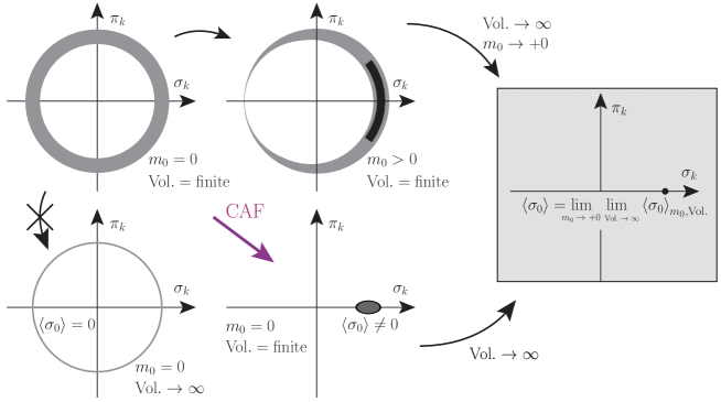
Figure 1: Schematic picture of CAF method. In order to obtain the chiral condensate rigorously, we need to put a finite mass, first take thermodynamic limit and finally take the chiral (massless) limit as shown in the upper panels. In CAF, we take chiral rotation to make the $\pi_{0}$ field vanish, and we get the finite chiral condensate (center bottom panel), which would be close to the correct value.

We here propose a chiral angle fixing (CAF) method as a prescription to calculate the chiral condensate on a fixed finite size lattice. The effective action Eq. (9) is invariant under the chiral transformation,

$$\chi_{x}\to\chi_{x}^{\prime}=e^{i\varepsilon_{x}\alpha/2}\chi_{x}\ ,\quad{\bar{\chi}}_{x}\to{\bar{\chi}}_{x}^{\prime}=e^{i\varepsilon_{x}\alpha/2}{\bar{\chi}}_{x}\ .$$ (21)

The chiral symmetry is kept in the bosonized effective action by introducing the chiral U(1) transformation for auxiliary fields as,

$$\begin{pmatrix}\sigma_{k}\\ \pi_{k}\end{pmatrix}\to\begin{pmatrix}\sigma_{k}^{\prime}\\ \pi_{k}^{\prime}\end{pmatrix}=\begin{pmatrix}\cos\alpha&-\sin\alpha\\ \sin\alpha&\cos\alpha\end{pmatrix}\begin{pmatrix}\sigma_{k}\\ \pi_{k}\end{pmatrix}\ ,$$ (22)

where $(\sigma_{k},\pi_{k})$ are the temporal Fourier transform of $(\sigma_{{{\mathbb{k}},\tau}},\pi_{{\mathbb{k}},\tau})$,

$$\sigma_{k=({\mathbb{k}},\omega)}= \frac{1}{N_{\tau}}\sum_{\tau}e^{-i\omega\tau}\sigma_{{\mathbb{k}},\tau}\ ,$$ (23)

$$\pi_{k=({\mathbb{k}},\omega)}= \frac{1}{N_{\tau}}\sum_{\tau}(-1)^{\tau}e^{-i\omega\tau}\pi_{{\mathbb{k}},\tau}=\frac{1}{N_{\tau}L^{3}}\sum_{x}e^{-ik\cdot x}\pi_{x}\ .$$ (24)

Because of the chiral symmetry, the chiral condensate $\langle{\sigma_{0}}\rangle$ vanishes as long as the auxiliary field configurations are taken to be chiral symmetric, as explicitly shown in Appendix B.

In order to avoid the vanishing chiral condensate, we here utilize CAF. We rotate $\sigma_{0}$ and $\pi_{0}$ modes toward the positive $\sigma_{0}$ direction as schematically shown in Fig. 1. All the other fields are rotated with the same angle, $-\alpha=-\arctan(\pi_{0}/\sigma_{0})$, in each Monte-Carlo configuration. We use these new fields to obtain order parameters, susceptibilities, and other quantities, and eventually obtain finite chiral condensate. Chiral condensate obtained in CAF should mimic the spontaneously broken chiral condensate in the thermodynamic limit. Similar prescriptions are adopted in other field of physics. For example, we take a root mean square order parameter to obtain the appropriate value in spin systems MCsim1 .

3.2 Sampling and Errors

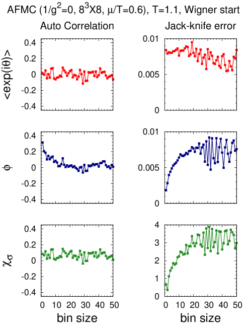
Figure 2: Autocorrelation (left column) and jack-knife error (right column) of average phase factor (top row), chiral condensate (middle row) and chiral susceptibility (bottom row) as a function of bin size for $\mu/T=0.6,\ T=1.1$ on a $8^{3}\times 8$ lattice starting from the Wigner phase initial condition. We adopt the saturated values after autocorrelations disappear as the errors of calculated quantities.

We generate auxiliary field configurations by using the Metropolis sampling method. We generate Markov chains starting from two types of initial conditions: the Wigner phase ($\sigma_{x}=0.01,\ \pi_{x}=0$) and the Nambu-Goldstone (NG) phase ($\sigma_{x}=2,\ \pi_{x}=0$) initial conditions.

For each $\tau$, we generate a candidate auxiliary field configuration $(\sigma^{\prime}_{{{\mathbb{k}},\tau}},\pi^{\prime}_{{{\mathbb{k}},\tau}})$ by adding random numbers to the current configuration $(\sigma_{{{\mathbb{k}},\tau}},\pi_{{{\mathbb{k}},\tau}})$ for all spatial momenta ${\mathbb{k}}$ at a time, and judge whether the new configuration is accepted or not by using the Metropolis algorithm. Since it is time consuming to update each auxiliary field mode separately, we update all spatial momentum modes in one step at the cost of an acceptance probability. We have tuned the strength (standard deviation) of the random numbers added to the current configuration $(\sigma_{{{\mathbb{k}},\tau}},\pi_{{{\mathbb{k}},\tau}})$ in order to keep the acceptance probability around 50 % at each $(T,\mu)$. It should be noted that the acceptance probability is larger in the present $(\sigma_{{{\mathbb{k}},\tau}},\pi_{{{\mathbb{k}},\tau}})$ sampling procedure in each $\tau$ compared with updating $(\sigma_{k},\pi_{k})$ in the whole momentum space at a time as done in our preliminary work Ohnishi:2012yb . For example, on a $4^{3}\times 4$ lattice at around the critical temperature at $\mu=0$, we find that the acceptance probability decreases to $15-20$ % in the $(\sigma_{k},\pi_{k})$ sampling from $\sim 50\%$ in the $(\sigma_{{{\mathbb{k}},\tau}},\pi_{{{\mathbb{k}},\tau}})$ sampling, when we adopt the same standard deviation. On a larger lattice, the acceptance probability difference in the two sampling methods would be larger.

We evaluate errors of calculated quantities in the jack-knife method JK . The evaluated errors of the chiral condensate $\phi$ are shown as a function of bin size in the right middle panel of Fig. 2. Since the Metropolis samples are generated sequentially in the Markov chain, subsequent events are correlated. This autocorrelation disappears when the Metropolis time difference is large enough. In the jack-knife method, we group the data into bins and regard the set of configurations except for those in a specified bin as a jack-knife sample. We find that the autocorrelation disappears for the bin size larger than 30 in this case. The jack-knife error increases with increasing bin size, and eventually saturates. We adopt the saturated value of the jack-knife error after the autocorrelation disappears as the error of the calculated quantity as in the standard jack-knife treatment. The errors are found to be small enough to discuss the phase transition. For example we find $\Delta\phi\lesssim 0.01$ in Fig. 2, and the value is small compared with its mean value $\phi\simeq 0.08$ shown in Fig. 3.

3.3 Order Parameters

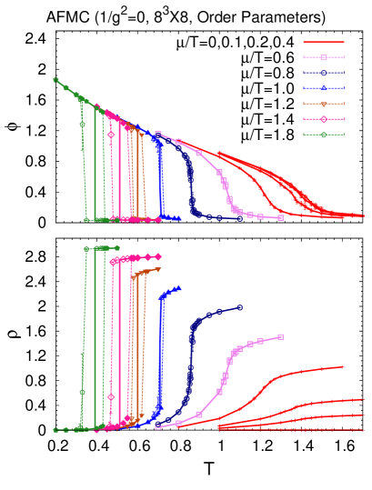
Figure 3: Chiral condensate (upper panel) and quark number density (lower panel) as a function of temperature ($T$) for a fixed $\mu/T(0\leq\mu/T\leq 1.8)$ on a $8^{3}\times 8$ lattice. Open symbols, filled symbols and lines show the results with the Wigner and NG initial conditions and those in the realized phase, respectively.

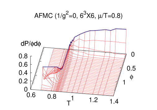
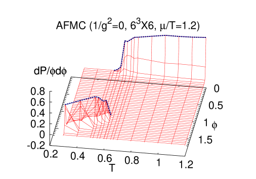
Figure 4: Chiral condensate ($\phi$) distribution as a function of temperature ($T$) and $\phi$ on a $6^{3}\times 6$ lattice for $\mu/T=0.8$ (top panel) and 1.2 (bottom panel).

In Fig. 3, we show the chiral condensate, $\phi=\left<\sigma_{0}\right>$, and the quark number density $\rho_{q}$ after CAF,

$$\left<\sigma_{0}\right>= \frac{1}{L^{3}N_{\tau}}\,\frac{\partial\ln Z}{\partial m_{0}}=-\left<{\bar{\chi}}\chi\right>\ ,$$ (25)

$$\rho_{q}= \frac{T}{L^{3}}\,\frac{\partial\ln Z}{\partial\mu}\ ,$$ (26)

as a function of temperature ($T$) on a $8^{3}\times 8$ lattice. Necessary formulae to obtain these quantities are summarized in Appendix C. We also show the distribution of $\phi$ in Fig. 4.

The order parameters, $\phi$ and $\rho_{q}$, clearly show the phase transition behavior. With increasing $T$ for fixed $\mu/T$, the chiral condensate $\phi$ slowly decreases at low $T$, shows rapid or discontinuous decrease at around the transition temperature, and stays to be small at higher $T$. The quark number density $\rho_{q}$ also shows the existence of phase transition at finite $\mu$.

The order of the phase transition can be deduced from the behavior of $\phi$, $\rho_{q}$ and the $\phi$ distribution on a small lattice Ohnishi:2012yb ; Ichihara:2013pc . The chiral condensate $\phi$ and the quark number density $\rho_{q}$ smoothly change around the (pseudo-)critical temperature ($T_{c}$) at small $\mu/T$. Additionally, the $\phi$ distribution has a single peak as shown in the top panel of Fig. 4. These observations suggest that the phase transition is crossover or the second order at small $\mu/T$ on a large size lattice. We refer to this $\mu/T$ region as the would-be second order region.

By comparison, the order parameters show hysteresis behavior in the large $\mu/T$ region. As shown by dashed lines in Fig. 3, two distinct results of $\phi$ and $\rho_{q}$ depend on the initial conditions, the Wigner phase and the NG phase initial conditions. The temperature of sudden $\phi$ change for the NG initial condition is larger than that for the Wigner initial condition. The distribution of $\phi$ shows a double peak as shown in the bottom panel of Fig. 4. In terms of the effective potential, the dependence of initial conditions indicates that there exist two local minima, which are separated by a barrier. In the hysteresis region, the transition between the two local minima is suppressed by the barrier and Metropolis samples stay around the local minimum close to the initial condition. At the temperature of sudden $\phi$ change, the barrier height becomes small enough for the Metropolis samples to overcome. These results suggest that the phase transition is the first order at large $\mu/T$. We refer to this $\mu/T$ region as the would-be first order region.

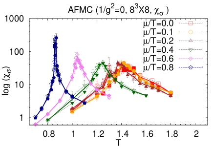
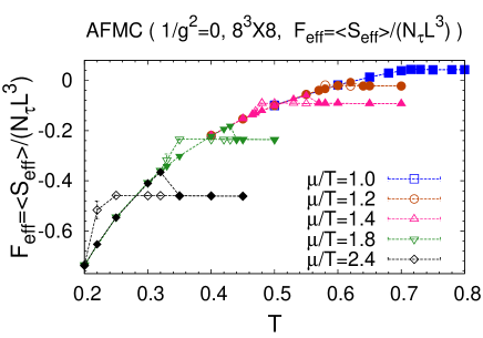
Figure 5: Chiral susceptibility $\chi_{\sigma}$ (left panel) and effective potential $F_{\mathrm{eff}}=\left<S_{\mathrm{eff}}\right>/(N_{\tau}L^{3})$ (right panel) as a function of temperature on a $8^{3}\times 8$ lattice. We determine the phase boundary by using $\chi_{\sigma}$ in the would-be 2nd order region and $F_{\mathrm{eff}}$ in the would-be 1st order region. Open symbols and filled symbols show results with the Wigner and NG initial conditions, respectively.

3.4 Phase Diagram

We shall now discuss the QCD phase diagram in AFMC. In Fig. 6, we show the QCD phase diagram for various lattice sizes. We define the (pseudo-)critical temperature $T_{c}$ as a peak position of the chiral susceptibility $\chi_{\sigma}$ ($=\partial^{2}\ln Z/\partial m_{0}^{2}/L^{3}N_{\tau}$, see also Appendix C) shown in Fig. 5 in the would-be second order region. We determine the peak position by fitting the susceptibility with a quadratic function. The errors are comprised of both statistical and systematic errors. We fit $\chi_{\sigma}$ as a function of $T$ with statistical errors obtained in the jack-knife method. In order to evaluate the systematic error, we change the fitting range as long as the fitted quadratic function describes an appropriate peak position. We take notice that we do not fit $\chi_{\sigma}$ as a function of $T$ in each jack-knife sample.

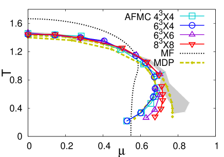
Figure 6: Phase diagram in AFMC on $4^{3}\times 4$, $6^{3}\times N_{\tau}$ $(N_{\tau}=4,6)$ and $8^{3}\times 8$ lattices. Short- and long-dashed lines show the mean-field (MF) MF-SCL ; NLOPD ; NNLO and the monomer-dimer-polymer (MDP) results MDP ; PhDFromm , respectively. Two lines in MDP show the results for $N_{\tau}=4$ (the left line) and those extrapolated to $N_{\tau}\to\infty$ (the right line). Shaded area shows the phase boundary extrapolated to $N_{\tau}\to\infty$ in AFMC.

In the would-be first order region of $\mu/T$, we determine the phase boundary by comparing the expectation values of effective action $\langle{S_{\mathrm{eff}}}\rangle$ in the configurations sampled from the Wigner and NG phase initial conditions. We define $T_{c}$ as the temperature where $\langle{S_{\mathrm{eff}}}\rangle$ with the Wigner initial condition becomes lower than that with the NG initial condition as shown in Fig. 5. We have adopted this prescription, since it is not easy to obtain equilibrium configurations over the two phases when the thermodynamic potential barrier is high. At large $\mu/T$, Metropolis samples in one sequence stay in the local minimum around the initial condition, and we need very large sampling steps to overcome the barrier.

In Fig. 6, we compare the AFMC phase boundary with that in the mean field approximation MF-SCL ; NLOPD ; NNLO and in the MDP simulation MDP ; PhDFromm in the strong coupling limit. Compared with the MF results, $T_{c}$ at low $\mu$ is found to be smaller, and NG phase is found to be extended in the finite $\mu$ region in both MDP MDP ; PhDFromm and AFMC. As found in previous works Ohnishi:2012yb ; Ichihara:2013pc , the phase boundary is approximately independent of the lattice size in the would-be second order region. The would-be first order phase boundary is insensitive to the spatial lattice size but is found to depend on the temporal lattice size. With increasing temporal lattice size, the transition chemical potential $\mu_{c}$ becomes larger, which is consistent with MDP MDP . Phase boundary extrapolated to $N_{\tau}\to\infty$ is obtained by assuming that the spatial size dependence is negligible. The extrapolated boundary is shown by the shaded area, and is found to be consistent with the continuous time MDP results with the same limit, $N_{\tau}\to\infty$ with keeping $\gamma^{2}/N_{\tau}$ finite.

Spatial lattice size independence of the phase boundary may be understood as a consequence of almost decoupled pions. The zero momentum pion can be absorbed into the chiral condensate via the chiral rotation and has no effects on the transition. Finite momentum pion modes have finite excitation energy, then we do not have soft modes in the would-be first order region on a small size lattice. For a more serious estimate of the size dependence, we need larger lattice calculations.

We find that the would-be first order phase boundary has a positive slope, $d\mu/dT>0$, at low $T$. The Clausius-Clapeyron relation reads $d\mu/dT|_{\mathrm{1st}}=-(s^{\mathrm{W}}-s^{\mathrm{NG}})/(\rho_{q}^{\mathrm{W}}-\rho_{q}^{\mathrm{NG}})$, where $s^{\mathrm{W,NG}}$ and $\rho_{q}^{\mathrm{W,NG}}$ are the entropy density and quark number density in the Wigner and NG phases, respectively. Since $\rho_{q}$ is higher in the Wigner phase as shown in Fig. 3, the entropy density should be smaller in the Wigner phase. This is because $\rho_{q}$ is close to the saturated value, $\rho_{q}\sim 3=N_{c}$, in the Wigner phase, then the entropy is carried by the hole from the fully saturated state. Similar behavior is found in the mean-field treatment in the strong coupling limit MF-SCL . In order to avoid the quark number density saturation, which is a lattice artifact, we may need to adopt a larger $N_{\tau}$ MDP or to take account of finite coupling effects NLOchiral ; NLOPD ; Bilic ; BilicDeme ; Faldt ; Jolicoeur ; NNLO .

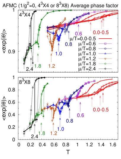
Figure 7: Average phase factor on $4^{3}\times 4$ (top panel) and $8^{3}\times 8$ (bottom panel) lattices as a function of temperature. Open symbols, filled symbols and lines show the results with the Wigner and NG initial conditions and those in the realized phase, respectively. Arrows indicate phase transition temperatures, and the numbers under arrows represent $\mu/T$.

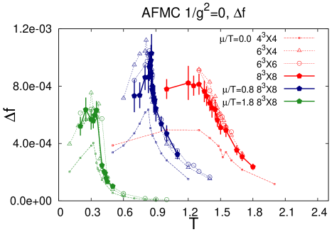
Figure 8: Free energy density difference $\Delta f$ in full and phase quenched simulations as a function of temperature on $4^{3}\times 4$, $6^{3}\times 4$, $6^{3}\times 6$ and $8^{3}\times 8$ lattices. We only show jack-knife errors with $8^{3}\times 8$ lattice results.

3.5 Average Phase Factor

In Fig. 7, we show the average phase factor $\left<e^{\mathrm{i}\theta}\right>$ as a function of $T$ on $8^{3}\times 8$ and $4^{3}\times 4$ lattices, where $\theta$ is a complex phase of the fermion determinant in each Monte-Carlo configuration. The average phase factor shows the severity of the weight cancellation; we have almost no weight cancellation when $\left<e^{\mathrm{i}\theta}\right>\simeq 1$, and the weight cancellation is severe in the cases where $\left<e^{\mathrm{i}\theta}\right>\simeq 0$. The average phase factor has a tendency to increase at large $\mu$ except for the transition region. This trend can be understood from the effective action in Eq. (20). The complex phase appears from $X_{N_{\tau}}$ terms containing auxiliary fields, and their contribution generally becomes smaller compared with the chemical potential term, $2\cosh(3N_{\tau}\mu/\gamma^{2})$, at large $\mu$. In the phase transition region, fluctuation effects of the auxiliary fields are decisive and finite momentum auxiliary fields might contribute significantly, which leads to a small average phase factor.

The average phase factor on a $4^{3}\times 4$ lattice, $\left<e^{\mathrm{i}\theta}\right>\gtrsim 0.9$, is practically large enough to keep statistical precision. By comparison, the smallest average phase factor on a $8^{3}\times 8$ lattice is around 0.1 at low temperature on a $\mu/T=2.4$ line. Even with this average phase factor, uncertainty of the phase boundary shown in Fig. 6 is found to be small enough to discuss the fluctuation effects.

We show the severity of the sign problem in AFMC in Fig. 8. The severity is characterized by the difference of the free energy density in full and phase quenched (p.q.) MC simulations, $\Delta f=f_{\mathrm{full}}-f_{\mathrm{p.q.}}$ which is related to the average phase factor, $e^{-\Omega\Delta f}=\left<e^{\mathrm{i}\theta}\right>$, where $\Omega=N_{\tau}L^{3}$ is the spacetime volume. While $\Delta f$ takes smaller values on a $4^{3}\times 4$ lattice than those on larger lattices, it takes similar values on lattices with larger spatial size $L\geq 6$. We expect that $\Delta f$ in AFMC for larger lattices would take values similar to those on a $8^{3}\times 8$ lattice.

We find that $\Delta f$ in AFMC is about twice as large as that in MDP when we compare the results at similar $(\mu,T)$ PhDFromm ; MDPsign . It means that the sign problem in AFMC is more severe than that in MDP. It is desired to develop a scheme to reduce $\Delta f$ in AFMC on larger lattices. In Sec. 4.2, we search for a possible way to weaken the weight cancellation by cutting off high momentum auxiliary fields.

4 Discussion

4.1 Volume Dependence of Chiral Susceptibility

We perform a finite size scaling analysis of the chiral susceptibility to discuss the phase transition order in the low chemical potential region. We expect that the phase transition is the second order at small $\mu/T$ according to the mean-field results and O(2) symmetry arguments. The latter states that the fluctuation induced first order phase transition is not realized as for O(2) symmetry PW84 .

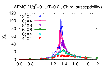
Figure 9: Lattice size dependence of the chiral susceptibility for $\mu/T=0.2$. Squares, circles, triangles, upside-down triangles, diamonds, and pentagons show the results on $4^{3}\times 4,\ 6^{3}\times 4,\ 6^{3}\times 6,\ 10^{3}\times 4$, and $12^{3}\times 4$ lattices, respectively. The peak height depends on spatial lattice size.

In Fig. 9, we show the chiral susceptibility for fixed $\mu/T=0.2$ on various size lattices. In addition to $4^{3}\times 4,\ 6^{3}\times 4,\ 6^{3}\times 6$ and $8^{3}\times 8$ results, we also show larger lattice results, $10^{3}\times 4$, and $12^{3}\times 4$. From this comparison, we find that $\chi_{\sigma}$ has a peak at the same $T$ for different lattice sizes, and that the peak height on $6^{3}\times 4$ and $6^{3}\times 6$ lattices are almost the same. These two findings suggest that it is reasonable to define the temperature as $T=\gamma^{2}/N_{\tau}$ in the strong coupling limit. We also find that the peak height of the susceptibility increases with increasing spatial lattice size. The divergence of the susceptibility in the thermodynamic limit signals the first or second order phase transition.

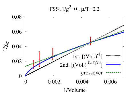
Figure 10: Finite size scaling of chiral susceptibility for $\mu/T=0.2$. Dotted, solid, and dashed lines show expected behavior of the first, second, and crossover transitions. We show chiral susceptibilities on the $6^{3}\times 4,6^{3}\times 6,8^{3}\times 8,10^{3}\times 4$, and $12^{3}\times 4$ lattices.

In order to find the finite size scaling of the chiral susceptibility FSS , we plot $1/\chi_{\sigma}$ at the peak as functions of inverse spatial lattice volume in Fig. 10. The chiral susceptibility is proportional to spatial volume $V=L^{3}$ in the first order phase transition region and to $V^{(2-\eta)/3}$ in the second order phase transition region for $d=3$ O(2) spin systems, where the O(2) critical exponent is $\eta=0.0380(4)$ criticalexp . By comparison, $\chi_{\sigma}$ does not diverge when the transition is crossover. It seems to suggest that the chiral phase transition at low $\mu$ is not the first order, and we cannot exclude the possibility of the crossover transition with the present precision in comparison with the above three scaling functions shown in Fig. 10 in AFMC. The current analysis implies that the phase transition is the second order or crossover phase transition. In order to conclude the order of the phase transition firmly, we need higher-precision and larger volume calculations.

4.2 High momentum mode contributions

We quantitatively examine the influence of high momentum auxiliary field modes on the average phase factor and the order parameters. For this purpose, we compare the results by cutting off high momentum auxiliary field modes having $\sum_{j}\sin^{2}k_{j}>\Lambda$, where $\Lambda$ is a cutoff parameter. The parameter $\Lambda$ is varied in the range $0\leq\Lambda\leq d=3$ to examine their cutoff effects; we include all Monte-Carlo configurations for $\Lambda=3$, while we only take account of the lowest momentum modes for $\Lambda=0$.

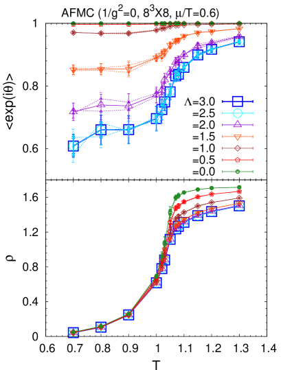
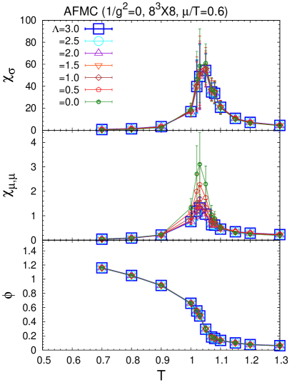
Figure 11: Cutoff parameter $\Lambda$ dependence as a function of temperature $T$ on a $8^{3}\times 8$ lattice on a fixed $\mu/T=0.6$ line in the chiral limit. We show the average phase factor (left top), quark number density (left bottom), chiral susceptibility (right top), quark number susceptibility (right middle), and chiral condensate (right bottom). Squares, big open circles, triangles, upside-down triangles, diamonds, pentagons and small filled circles show results for $\Lambda=3,2.5,2,1.5,1,0.5$ and 0, respectively.

The average phase factor might become large in the cases where high momentum mode contributions are negligible as discussed in Sec. 2.2, so we anticipate that the weight cancellation becomes weaker for smaller $\Lambda$. In the left top panel of Fig. 11, we show the $\Lambda$ dependence of the average phase factor on a $8^{3}\times 8$ lattice for $\mu/T=0.6$. The average phase factor has a large value when $\Lambda\rightarrow 0$, where we improve the weight cancellation. These results are consistent with our expectation for the weight cancellation with high momentum modes. We could here conclude that high momentum modes are closely related to severe weight cancellation.

In the right bottom panel of Fig. 11, we show the chiral condensate $\phi$ on a $8^{3}\times 8$ lattice for $\mu/T=0.6$. We here utilize $\phi=\left<\sum_{\tau}\sigma_{\bm{k}=\bm{0},\tau}/N_{\tau}\right>$. This expression is equivalent to Eq. (25) for $\Lambda=3$. The chiral condensate does not depend on the parameter $\Lambda$ since the lowest modes of the integration variables ($\sigma_{{\mathbb{k}},\tau},\ \pi_{{\mathbb{k}},\tau}$) in AFMC consist of the scalar and pseudoscalar modes. In Fig. 11, we also plot the cutoff dependence of other quantities: quark number density ($\rho_{q}$), chiral susceptibility ($\chi_{\sigma}$) and quark number susceptibility ($\chi_{\mu,\mu}$). We find that these quantities do not strongly depend on the cutoff as long as $\Lambda\geq 2$. By contrast, the quantities are affected by the cutoff parameter for $\Lambda<2$. We have already found that the average phase factor becomes large if we set $\Lambda\leq 2.5$. Thus, this analysis implies a probable presence of an optimal cutoff $\Lambda_{\mathrm{o}}$, with which the order parameter values are almost the same as those of the all momentum modes and the reliability of numerical simulation is improved. We conclude that there is a possible way to study the QCD phase diagram for larger lattice by cutting off or approximating the high momentum modes without changing the behavior of the order parameters.

5 Summary

We have investigated the QCD phase diagram and the sign problem in the auxiliary field Monte-Carlo (AFMC) method with chiral angle fixing (CAF) technique. In order to obtain the auxiliary field effective action, we first integrate out spatial link variables and obtain an effective action as a function of quark fields and temporal link variables in the leading order of the $1/g^{2}$ and $1/d$ expansion with one species of unrooted staggered fermion. By using the extended Hubbard-Stratonovich (EHS) transformation, we convert the four-Fermi interactions into the bilinear form of quarks. The auxiliary field effective action is obtained after analytic integration over the quark and temporal link variables. We have performed the auxiliary field integral using the Monte-Carlo technique.

We have obtained auxiliary field configurations in AFMC and the order parameters: the chiral condensate and quark number density. Both of these order parameters show phase transition behavior. In the low chemical potential region, the chiral condensate decreases smoothly with increasing temperature, while the quark number density increases gently. This behavior suggests that the phase transition is the second order or crossover, which is consistent with the analysis of the distribution of the chiral condensate. We call the low chemical potential region the would-be second order region. In order to deduce the phase boundary, we here define (pseudo-)critical temperature as a peak position of the chiral susceptibility. One finds that the critical temperature is suppressed compared with the mean-field results on an isotropic lattice MF-SCL ; NLOPD ; NNLO and is almost independent of lattice size as shown in the monomer-dimer-polymer simulations (MDP) at the would-be second order phase transition MDP ; PhDFromm . We also give some results of finite size scaling to guess the phase transition order. While one could expect the second order phase transition from the mean-field and O(2) symmetry arguments in the low chemical potential region, it is not yet conclusive to decide whether the transition is the second order or crossover at the present precision.

At high chemical potential, the order parameters show sudden jump and hysteresis, and depend on initial conditions: the Wigner and Nambu-Goldstone initial conditions. The distribution of the chiral condensate has a double peak around the phase transition region. These results imply that the order of the phase transition is the first order owing to the existence of the two local minima with a relatively high barrier compared to the Metropolis jumping width. We call this phase transition the would-be first order phase transition in the present paper. We here regard transition temperature as a crossing point of the expectation value of the effective action with two initial conditions. According to our analysis, the Nambu-Goldstone phase is enlarged toward the high chemical potential region compared with the mean-field results. The phase boundary depends very weakly on spatial lattice size and more strongly on temporal lattice size. This behavior is also found in MDP MDP .

We find that we have a sign problem in AFMC. The origin of the weight cancellation is the bosonization of the negative modes in the extended Hubbard-Stratonovich (EHS) transformation; an imaginary number must be introduced in the fermion matrix. The fermion determinant becomes complex, and the weight cancellation arises when we numerically integrate auxiliary fields. In our framework, we have a phase cancellation mechanism for low momentum auxiliary fields; a phase on one site is canceled out by the nearest neighbor site phase. We quantitatively show that the high momentum modes contribute to the weight cancellation by cutting off these modes. We also confirm the cutoff dependence on order parameters and susceptibilities. We find that there is a cutoff parameter region where the behavior of the quantities are not altered from the all mode results and the weight cancellation is weakened. Therefore, there is a possibility to investigate phase transition phenomena using cutoff or approximation scheme for high momentum modes.

While we have a sign problem in AFMC, the weight cancellation is not serious on small lattices adopted here ($\sim 8^{3}\times 8$ size) because of the phase cancellation mechanism for the low momentum modes. The phase boundary in AFMC is found to be consistent with that in MDP MDP .

In this paper, we utilize CAF in order to obtain the order parameters and susceptibilities in the chiral limit on a fixed finite size lattice. The chiral condensate in finite volume should vanish in a rigorous sense due to the chiral symmetry between the scalar and pseudoscalar modes. In order to simulate the non-vanishing chiral condensate to be obtained in the rigorous procedure of the thermodynamic limit followed by the chiral limit, the chiral transformation of auxiliary fields are carried out in each configuration so as to fix the chiral angle in the real positive direction (positive scalar mode direction). We could evaluate the adequate chiral condensate and chiral susceptibility by using CAF.

The AFMC method could be straightforwardly applied to include finite coupling effects since bosonization technique is applied in the mean-field analysis NLOPD ; NNLO . Both fluctuations and finite coupling effects are important to elucidate features of the phase transition phenomena, so the AFMC would be a possible way to include these two effects at a time. The sign problem might be severer than that in the strong coupling limit when we include finite coupling effects. One of the promising methods to avoid lower numerical reliability is to invoke shifted contour formulation avoidsign , and another promising direction is to integrate over the Lefschetz thimbles thimble . We hope that we may apply the formulation with finite coupling effects or on a larger lattice. We also obtain appropriate order parameters in a relatively hassle-free CAF method compared to a rigorous way. In AFMC, chiral symmetry is respected manifestly. We expect that auxiliary fields for finite coupling terms also keep chiral symmetry manifestly, and CAF can be also applied to finite coupling cases. We might use this CAF method with higher-order corrections in the strong coupling expansion to investigate the phase diagram. It is also important to develop a method to include spatial baryon hopping terms and other higher order terms in the $1/d$ expansion in AFMC.

Appendix A Temporal-spatial lattice spacing ratio on an anisotropic lattice

In this paper, we have adopted the physical temporal-spatial lattice spacing ratio $f(\gamma)=a_{s}^{\mathrm{phys}}/a_{\tau}^{\mathrm{phys}}=\gamma^{2}$ given in Refs. Bilic ; BilicDeme ; PhDFromm . We briefly summarize the arguments given in these references.

In general, we can set temporal lattice spacing as $a_{\tau}^{\mathrm{phys}}(\gamma,g)=a_{s}^{\mathrm{phys}}/f(\gamma,g)$, where $f(\gamma,\infty)=f(\gamma)$ in SCL. In order to give the expression for the function $f$, we can impose two conditions that critical temperature $T_{c}=1/N_{\tau}a_{\tau}^{\mathrm{phys}}=f(\gamma)/N_{\tau}a_{{\color[rgb]{0,0,0}{s}}}^{\mathrm{phys}}$ should not depend on $N_{\tau}$, and that the hypercube symmetry is restored on an isotropic lattice, $a_{\tau}^{\mathrm{phys}}(1,g)=a_{s}^{\mathrm{phys}}$. Since the critical coupling $\gamma_{c}$ at $\mu=0$ is given as $\gamma^{2}_{c}/N_{\tau}=d(N_{c}+1)(N_{c}+2)/6(N_{c}+3)$ for $\mathrm{SU}(N_{c})$ with one species of unrooted staggered fermion in the mean field treatment in SCL, the above requirements suggest that the function $f$ should be given as $f(\gamma)=\gamma^{2}$.

This prescription seems to be valid also for high chemical potential region as long as $\gamma$ is bigger than unity. This is because critical chemical potential $\mu_{c}$ at zero temperature becomes constant as long as $\gamma\gg 1$ when we apply $f(\gamma)=\gamma^{2}$, which is consistent with the zero chemical potential result.

Appendix B Chiral Angle Fixing

We here discuss the chiral angle fixing (CAF) from another point of view. As mentioned in Sec. 3.1, the chiral condensate ideally disappears due to the chiral symmetry. We could confirm an aspect of CAF method as follows. According to a relation, $S(\phi_{\mathbf{k},\omega},\alpha_{\mathbf{k},\omega},\phi,\alpha)=S(\phi_{\mathbf{k},\omega},\alpha_{\mathbf{k},\omega}^{\prime}=\alpha_{\mathbf{k},\omega}-\alpha,\phi,0)$, where $\alpha$ is the chiral angle, the chiral condensate is given as

$$\left<\sigma_{0}\right>= \frac{1}{Z}\int\mathcal{D}\left[\sigma_{0},\pi_{0}\right]\ \prod_{(\mathbf{k},\omega)\not=(\bm{0},0)}\mathcal{D}\left[\sigma_{\mathbf{k},\omega},\pi_{\mathbf{k},\omega}\right]\ \sigma_{0}\ e^{-S(\sigma_{\mathbf{k},\omega},\pi_{\mathbf{k},\omega},\phi=\sqrt{\sigma_{0}^{2}+\pi_{0}^{2}},\alpha)}\$$

$$= \frac{1}{Z}\int\mathcal{D}\left[\phi,\alpha\right]\ \phi\cos\alpha\int\prod_{(\mathbf{k},\omega)\not=(\bm{0},0)}\mathcal{D}\left[\phi_{\mathbf{k},\omega},\alpha_{\mathbf{k},\omega}^{\prime}\right]\ e^{-S(\phi_{\mathbf{k},\omega},\alpha_{\mathbf{k},\omega}^{\prime},\phi,0)}$$

$$= 0\ .$$ (27)

$\phi_{\mathbf{k},\omega}$ and $\alpha_{\mathbf{k},\omega}$ are chiral radius and chiral angle of each chiral partner. We find that the chiral condensate ideally vanishes according to Eq. (27). In CAF, we rotate the negative chiral angle ($-\alpha$) with respect to all fields and set $\pi_{0}=0$. We obtain the finite chiral condensate in the Nambu-Goldstone (NG) phase as

$$\left<\sigma_{0}\right>= \frac{1}{Z}\int\mathcal{D}\sigma_{0}\ \sigma_{0}\int\prod_{(\mathbf{k},\omega)\not=(\bm{0},0)}\mathcal{D}\left[\phi_{\mathbf{k},\omega},\alpha_{\mathbf{k},\omega}\right]\ \ e^{-S(\phi_{\mathbf{k},\omega},\alpha_{\mathbf{k},\omega},\phi=\sigma_{0},0)}$$

$$\neq 0\ .$$ (28)

The resultant chiral condensate in CAF should simulate the spontaneously broken chiral condensate in the thermodynamic limit. In the Wigner phase, $\left<\sigma_{0}\right>$ after CAF takes a finite value on the finite size lattice, but it decreases with increasing lattice size as shown in Fig. 12. In the limit of infinite volume, we could expect that the chiral condensate approaches zero in the Wigner phase, as expected in the continuum theories.

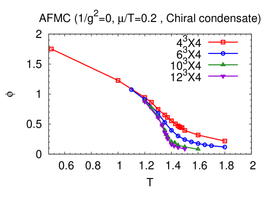
Figure 12: Spatial lattice size dependence of the chiral condensate on the $\mu/T=0.2$ line. In the Wigner phase, the chiral condensate decreases with increasing spatial lattice size.

We have some advantages in CAF. One is that the chiral condensate is finite in the NG phase and the chiral susceptibility may have a peak. In the cases where the chiral condensate vanishes ($\left<\sigma_{0}\right>=0$), the chiral susceptibility, $\chi_{\sigma}=\left<\sigma_{0}^{2}\right>-\left<\sigma_{0}\right>^{2}$, becomes $\chi_{\sigma}\rightarrow\left<\sigma_{0}^{2}\right>$, then we could expect that the chiral susceptibility increases with lower temperature. After we utilize CAF, we obtain the chiral susceptibility with a peak because of the non-vanishing chiral condensate at low $T$ as shown in Fig. 9. Another merit of CAF is that when we calculate the chiral condensate and the chiral susceptibility, we could take into account the information on the pseudoscalar mode which is mixed with scalar mode in the chiral limit.

Appendix C Recursion formula, Order parameters & Susceptibilities

C.1 Recursion formula

First, we shortly introduce a matrix to confirm notation Faldt ; Bilic ; BilicDeme . The function, $B_{N_{\tau}}$, is defined as

$$B_{N_{\tau}}(I_{1},\cdots,I_{N_{\tau}})=\left|\begin{array}[]{ccccc}I_{1}&e^{\mu/\gamma^{2}}&0&\cdots&0\\ -e^{-\mu/\gamma^{2}}&I_{2}&e^{\mu/\gamma^{2}}&&\vdots\\ 0&-e^{-\mu/\gamma^{2}}&I_{3}\cdot&\ddots&\vdots\\ \vdots&0&\ddots&\ddots&0\\ \vdots&\ddots&\ddots&I_{N_{\tau}-1}&e^{\mu/\gamma^{2}}\\ 0&\cdots&0&-e^{-\mu/\gamma^{2}}&I_{N_{\tau}}\\ \end{array}\right|\ ,\$$ (35)

where $I_{x}=2m_{x}/\gamma$. In the mean-field approximation, $I_{i}=\mathrm{const.}$ for any $i$. By comparison, $I_{i}$ depends on the spacetime when fluctuations are taken into account, therefore $I_{i}\neq I_{j}$ for $i\neq j$. Using Eq. (35), $B_{N_{\tau}}$ can be written in recursion formulae Faldt ; Bilic ; BilicDeme ,

$$B_{N_{\tau}}\left(I_{1},\cdots,I_{N_{\tau}}\right) =I_{N_{\tau}}B_{N_{\tau}-1}\left(I_{1},\cdots,I_{N_{\tau}-1}\right)+B_{N_{\tau}-2}\left(I_{1},\cdots,I_{N_{\tau}-2}\right)\ ,$$ (36)

where $B_{1}=I_{1}$, $B_{2}=I_{1}I_{2}+1$. $X_{N_{\tau}}$ in Eq. (20) is obtained by using $B_{N_{\tau}}$ as

$$X_{N_{\tau}}\left(I_{1},\cdots,I_{N_{\tau}}\right) =B_{N_{\tau}}\left(I_{1},\cdots,I_{N_{\tau}}\right)+B_{N_{\tau}-2}\left(I_{2},\cdots,I_{N_{\tau}-1}\right)\ .$$ (37)

In this paper, we numerically calculate $X_{N_{\tau}}$ and $B_{N_{\tau}}$ by using these recursion formulae.

C.2 Order parameters and Susceptibilities

We here summarize the expression for order parameters and susceptibilities Faldt . The chiral condensate $\langle$ $\sigma_{0}$ $\rangle$ and the chiral susceptibility $\chi_{\sigma}$ are described as

$$\left<\sigma_{0}\right>= -\frac{1}{L^{3}N_{\tau}}\frac{\partial\ln Z}{\partial m_{0}}=-\frac{1}{L^{3}N_{\tau}}\frac{1}{Z}\int\mathcal{D}\left[\sigma,\pi\right]\left(-\frac{\partial S_{\mathrm{eff}}^{\mathrm{AF}}}{\partial m_{0}}\right)e^{-S_{\mathrm{eff}}^{\mathrm{AF}}}=\frac{1}{L^{3}N_{\tau}}\left<\frac{\partial S_{\mathrm{eff}}^{\mathrm{AF}}}{\partial m_{0}}\right>\ ,$$ (38)

$$\chi_{\sigma}= \frac{1}{L^{3}N_{\tau}}\frac{\partial^{2}\ln Z}{\partial m_{0}^{2}}=\frac{1}{L^{3}N_{\tau}}\left[\left<\left(\frac{\partial S_{\mathrm{eff}}^{\mathrm{AF}}}{\partial m_{0}}\right)^{2}\right>-\left<\frac{\partial S_{\mathrm{eff}}^{\mathrm{AF}}}{\partial m_{0}}\right>^{2}-\left<\frac{\partial^{2}S_{\mathrm{eff}}^{\mathrm{AF}}}{\partial m_{0}^{2}}\right>\right]$$

$$= \frac{1}{L^{3}N_{\tau}}\left[\left<\left(\frac{\partial S_{\mathrm{eff}}^{\mathrm{AF}}}{\partial m_{0}}-\left<\frac{\partial S_{\mathrm{eff}}^{\mathrm{AF}}}{\partial m_{0}}\right>\right)^{2}\right>-\left<\frac{\partial^{2}S_{\mathrm{eff}}^{\mathrm{AF}}}{\partial m_{0}^{2}}\right>\right]\ ,$$ (39)

where $Z=\int\mathcal{D}\left[\sigma,\pi\right]\exp\left(-S_{\mathrm{eff}}^{\mathrm{AF}}\right)$. The derivatives of the effective action in Eq. (38) and (39) are given as

$$\frac{\partial S_{\mathrm{eff}}^{\mathrm{AF}}}{\partial m_{0}}= -\sum_{\bm{x}}\frac{\partial\ln\mathcal{\mathcal{K}}}{\partial m_{0}}=-\sum_{\bm{x}}\frac{1}{\mathcal{K}}\frac{\partial I_{x}}{\partial m_{0}}\frac{\partial X_{N_{\tau}}}{\partial I_{x}}\frac{\partial\mathcal{K}}{\partial X_{N_{\tau}}}$$

$$= -\sum_{\bm{x}}\frac{1}{\mathcal{K}}\frac{2}{\gamma}\sum_{t}B_{N_{\tau}-1}\left(I_{t+1},\cdots,I_{N_{\tau}},I_{1},\cdots,I_{t-1}\right)\left(3X_{N_{\tau}}^{2}-2\right)\ ,$$ (40)

$$\frac{\partial^{2}S_{\mathrm{eff}}^{\mathrm{AF}}}{\partial m_{0}^{2}}= \sum_{\bm{x}}\left[\frac{1}{\mathcal{K}^{2}}\left(\frac{2}{\gamma}\sum_{t}B_{N_{\tau}-1}\left(I_{t+1},\cdots,I_{N_{\tau}},I_{1},\cdots,I_{t-1}\right)\left(3X_{N_{\tau}}^{2}-2\right)\right)^{2}\right.$$

$$-\frac{1}{\mathcal{K}}\left(\frac{2}{\gamma}\right)^{2}\sum_{t,t^{\prime}}\left\{\sum_{t>t^{\prime}}B_{N-t+t^{\prime}-1}(I_{t+1},\cdots,I_{N},I_{1},\cdots,I_{t^{\prime}-1})B_{t-t^{\prime}-1}(I_{t^{\prime}+1},\cdots,I_{t-1})\right.$$

$$\left.+\sum_{t<t^{\prime}}B_{t^{\prime}-t-1}(I_{t+1},\cdots,I_{t^{\prime}-1})B_{N-t^{\prime}+t-1}(I_{t^{\prime}+1},\cdots,I_{N},I_{1},\cdots,I_{t-1})\right\}\left(3X_{N_{\tau}}^{2}-2\right)$$

$$\left.-\frac{1}{\mathcal{K}}\frac{24}{\gamma^{2}}X_{N_{\tau}}\left(\sum_{t}B_{N_{\tau}-1}\left(I_{t+1},\cdots,I_{N_{\tau}},I_{1},\cdots,I_{t-1}\right)\right)^{2}\right]\ ,$$ (41)

where $\mathcal{K}=X_{N_{\tau}}^{3}-2X_{N_{\tau}}+2\cosh(3N_{\tau}\mu/\gamma^{2})$. Similarly, we also obtain quark number density $\rho_{q}$, quark number susceptibility $\chi_{\mu,\mu}$ and mixed susceptibility $\chi_{m_{0},\mu}$

$$\rho_{q}= -\frac{T}{L^{3}}\frac{\partial\ln Z}{\partial\mu}=\frac{T}{L^{3}}\left<\frac{\partial S_{\mathrm{eff}}^{\mathrm{AF}}}{\partial\mu}\right>\ ,$$ (42)

$$\chi_{\mu,\mu}= \frac{1}{L^{3}N_{\tau}}\frac{\partial^{2}\ln Z}{\partial\mu^{2}}=\frac{1}{L^{3}N_{\tau}}\left[\left<\left(\frac{\partial S_{\mathrm{eff}}^{\mathrm{AF}}}{\partial\mu}-\left<\frac{\partial S_{\mathrm{eff}}^{\mathrm{AF}}}{\partial\mu}\right>\right)^{2}\right>-\left<\frac{\partial^{2}S_{\mathrm{eff}}^{\mathrm{AF}}}{\partial\mu^{2}}\right>\right]\ ,$$ (43)

$$\chi_{m_{0},\mu}= \frac{1}{L^{3}N_{\tau}}\frac{\partial^{2}\ln Z}{\partial\mu\partial m_{0}}=\frac{1}{L^{3}N_{\tau}}\left[\left<\frac{\partial S_{\mathrm{eff}}^{\mathrm{AF}}}{\partial m_{0}}\cdot\frac{\partial S_{\mathrm{eff}}^{\mathrm{AF}}}{\partial\mu}\right>-\left<\frac{\partial S_{\mathrm{eff}}^{\mathrm{AF}}}{\partial m_{0}}\right>\left<\frac{\partial S_{\mathrm{eff}}^{\mathrm{AF}}}{\partial\mu}\right>-\left<\frac{\partial^{2}S_{\mathrm{eff}}^{\mathrm{AF}}}{\partial m_{0}\partial\mu}\right>\right]\ ,$$ (44)

where

$$\frac{\partial S_{\mathrm{eff}}^{\mathrm{AF}}}{\partial\mu}= -\sum_{\bm{x}}\frac{\partial\ln\mathcal{\mathcal{K}}}{\partial\mu}=-\sum_{\bm{x}}\frac{1}{\mathcal{K}}\frac{2\cdot 3N_{\tau}}{\gamma^{2}}\sinh\left(\frac{3N_{\tau}\mu}{\gamma^{2}}\right)\ ,$$ (45)

$$\frac{\partial^{2}S_{\mathrm{eff}}^{\mathrm{AF}}}{\partial\mu^{2}}= \sum_{\bm{x}}\left[\frac{1}{\mathcal{K}^{2}}\left(\frac{2\cdot 3N_{\tau}}{\gamma^{2}}\sinh\left(\frac{3N_{\tau}\mu}{\gamma^{2}}\right)\right)^{2}-\frac{2}{\mathcal{K}}\left(\frac{3N_{\tau}}{\gamma^{2}}\right)^{2}\cosh\left(\frac{3N_{\tau}\mu}{\gamma^{2}}\right)\right]\ ,$$ (46)

$$\frac{\partial^{2}S_{\mathrm{eff}}^{\mathrm{AF}}}{\partial m_{0}\partial\mu}= \sum_{\bm{x}}\frac{1}{\mathcal{K}^{2}}\frac{2\cdot 3N_{\tau}}{\gamma^{2}}\sinh\left(\frac{3N_{\tau}\mu}{\gamma^{2}}\right)\left(\frac{2}{\gamma}\right)$$

$$\times\sum_{t}B_{N_{\tau}-1}\left(I_{t+1},\cdots,I_{N_{\tau}},I_{1},\cdots,I_{t-1}\right)\left(3X_{N_{\tau}}^{2}-2\right)\ .$$ (47)

References

- (1) Z. Fodor, S. D. Katz, JHEP 0203 (2002) 014; JHEP 0404 (2004) 050.
- (2) S. Ejiri et al., Prog. Theor. Phys. Suppl. 153 (2004) 118.
- (3) P. de Forcrand and O. Philipsen, Nucl. Phys. B 642 (2002) 290; M. D’Elia and M. -P. Lombardo, Phys. Rev. D 67 (2003) 014505;
- (4) S. Ejiri, Phys. Rev. D 78 (2008) 074507; A. Li, A. Alexandru and K. -F. Liu, Phys. Rev. D 84 (2011) 071503.
- (5) K. Nagata and A. Nakamura, Phys. Rev. D 82 (2010) 094027.
- (6) H. Saito et al. [WHOT-QCD Collaboration], Phys. Rev. D 84, 054502 (2011) [Erratum-ibid. D 85, 079902 (2012)].
- (7) G. Aarts, E. Seiler and I. -O. Stamatescu, Phys. Rev. D 81, 054508 (2010) [arXiv:0912.3360 [hep-lat]]; E. Seiler, D. Sexty, I. -O. Stamatescu, Phys. Lett. B 723, 213-216 (2013).
- (8) K. Splittorff, PoS LAT 2006, 023 (2006) [hep-lat/0610072]; J. Han and M. A. Stephanov, Phys. Rev. D 78, 054507 (2008) [arXiv:0805.1939 [hep-lat]]; M. Hanada and N. Yamamoto, JHEP 1202, 138 (2012) [arXiv:1103.5480 [hep-ph]]; Y. Hidaka and N. Yamamoto, Phys. Rev. Lett. 108, 121601 (2012) [arXiv:1110.3044 [hep-ph]].
- (9) D. T. Son and M. A. Stephanov, Phys. Rev. Lett. 86, 592 (2001); J. B. Kogut and D. K. Sinclair, Phys. Rev. D 70, 094501 (2004); P. de Forcrand, M. A. Stephanov and U. Wenger, PoS LAT2007, 237 (2007).
- (10) N. Kawamoto and J. Smit, Nucl. Phys. B192, 100 (1981); H. Kluberg-Stern, A. Morel, B. Petersson, Phys. Lett. B 114, 152 (1982); J. Hoek, N. Kawamoto, and J. Smit, Nucl. Phys. B 199, 495 (1982); P. H. Damgaard, N. Kawamoto and K. Shigemoto, Phys. Rev. Lett. 53, 2211 (1984); P. H. Damgaard, D. Hochberg, and N. Kawamoto, Phys. Lett. B 158, 239 (1985); P. H. Damgaard, N. Kawamoto, and K. Shigemoto, Nucl. Phys. B 264, 1 (1986); V. Azcoiti, G. Di Carlo, A. Galante, and V. Laliena, J. High Energy Phys. 09, 014 (2003).
- (11) H. Kluberg-Stern, A. Morel, B. Petersson, Nucl. Phys. B 215 [FS7], 527 (1983);
- (12) K. Fukushima, Prog. Theor. Phys. Suppl. 153, 204 (2004) [hep-ph/0312057]; Y. Nishida, Phys. Rev. D 69, 094501 (2004) [hep-ph/0312371].
- (13) G. Faldt and B. Petersson, Nucl. Phys. B 265, 197 (1986).
- (14) N. Bilic, K. Demeterfi and B. Petersson, Nucl. Phys. B 377, 651 (1992).
- (15) N. Bilic, F. Karsch, and K. Redlich, Phys. Rev. D 45, 3228 (1992); N. Bilic and J. Cleymans, Phys. Lett. B 355, 266 (1995).
- (16) T. Jolicoeur, H. Kluberg-Stern, M. Lev, A. Morel, and B. Petersson, Nucl. Phys. B 235, 455 (1984).
- (17) I. Ichinose, Phys. Lett. B135, 148 (1984); ibid. B147, 449 (1984); I. Ichinose, Nucl. Phys. B249, 715 (1985).
- (18) K. Miura, T. Z. Nakano and A. Ohnishi, Prog. Theor. Phys. 122, 1045 (2009) [arXiv:0806.3357 [nucl-th]]; K. Miura, T. Z. Nakano, A. Ohnishi and N. Kawamoto, Phys. Rev. D 80, 074034 (2009) [arXiv:0907.4245 [hep-lat]].
- (19) T. Z. Nakano, K. Miura and A. Ohnishi, Prog. Theor. Phys. 123, 825 (2010) [arXiv:0911.3453 [hep-lat]]; T. Z. Nakano, K. Miura and A. Ohnishi, Phys. Rev. D 83, 016014 (2011) [arXiv:1009.1518 [hep-lat]].
- (20) F. Karsch and K. H. Mutter, Nucl. Phys. B 313, 541 (1989).
- (21) P. de Forcrand and M. Fromm, Phys. Rev. Lett. 104, 112005 (2010) [arXiv:0907.1915 [hep-lat]]; W. Unger and P. de Forcrand, J. Phys. G 38, 124190 (2011) [arXiv:1107.1553 [hep-lat]].
- (22) M. Fromm, Ph.D. thesis, ETH-19297, Eidgenssische Technische Hochschule ETH Zrich, 2010.
- (23) M. Fromm, P. de Forcrand, PoS LATTICE2009, 193 (2009).
- (24) P. de Forcrand, J. Langelage, O. Philipsen, and W. Unger, PoS LATTICE2013, 142 (2013) [arXiv:1312.0589 [hep-lat]]; W. Unger, Acta Phys. Polon. Supp. 7 No. 1, 127 (2014).
- (25) M. Honma, T. Mizusaki and T. Otsuka, Phys. Rev. Lett. 75, 1284 (1995); T. Abe and R. Seki, Phys. Rev. C 79, 054002 (2009).
- (26) J. Carlson, S. Gandolfi and A. Gezerlis, PTEP 2012, 01A209 (2012) [arXiv:1210.6659 [nucl-th]].
- (27) B. Kurt and W. H. Dieter, Monte Carlo simulation in statistical physics: an introduction (Springer Verlag, Berlin, 2010), References therein.
- (28) S. A. Baeurle, R. Martonak, and M. Parrinello, J. Chem. Phys. 117, 3027 (2002); S. A. Baeurle, Phys. Rev. Lett. 89, 080602 (2002).
- (29) M. Cristoforetti, F. D. Renzo, and L. Scorzato [AuroraScience Collaboration], Phys. Rev. D 86, 074506 (2012) [arXiv:1205.3996 [hep-lat]]; H. Fujii, D. Honda, M. Kato, Y. Kikukawa, S. Komatsu and T. Sano, JHEP 1310, 147 (2013) [arXiv:1309.4371 [hep-lat]].
- (30) A. Ohnishi, T. Ichihara and T. Z. Nakano, PoS LATTICE2012, 088 (2012).
- (31) T. Ichihara, T. Z. Nakano, and A. Ohnishi, PoS LATTICE2013, 143 (2013).
- (32) For example, I. Montvay and G. Munster, Quantum Fields on a Lattice (Cambridge University Press, Cambridge, 1994)
- (33) R. D. Pisarski and F. Wilczek, Phys. Rev. D 29, 338 (1984).
- (34) Y. Aoki, G. Endrodi, Z. Fodor, S. D. Katz, and K. K. Szabo, Nature 443, 675 (2006); G. Endrodi, Z. Fodor, S. D. Katz, K. K. Szabo, JHEP 1104, 001 (2011).
- (35) M. Campostrini, M. Hasenbusch, A. Pelissetto, P. Rossi, and E. Vicari, Phys. Rev. B 63, 214503 (2001), cond-mat/0010360.