Slow and fast light dynamics in a chiral cold and hot atomic medium

Abstract

We study Chiral Based Electromagnetically Induced Transparency (CBEIT) of a light pulse and its associated subluminal and superluminal behavior through a cold and a hot medium of 4-level double-Lambda type atomic system. The dynamical behavior of this chiral based system is temperature dependent. The magnetic field based chirality and dispersion is always opposite as compared with the electric field ones. Contrastingly, the response of the chiral effect along with the incoherence Doppler broadening mechanism enhances the superluminal behavior as compared with its traditional degrading effect. Nevertheless, the intensity of a coupled microwave field destroys the coherence of the medium and degrade superluminality and subluminality of the sysmtem. The undistorted retrieved pulse from a hot chiral medium delays by $896ns$ than from a cold chiral medium under same set of parameters. Nevertheless, it advances by $-31ns$ in the cold chiral medium when a suitably different spectroscopic parameters are selected. The corresponding group index of the medium and the time delay/advance, are studied and analyzed explicitly [Note: A revise version is under preparation]

Quantum coherence is widely initiated through strong laser fields in multi-level atomic or molecular system interacting with electromagnetic fields. The coherent atomic or molecular states, which are prepared by the laser field, may then generates phenomenon of quantum interference among various transition amplitudes. The control over the response function of the media is then the result of the control of quantum coherence and interference effects. In the recent two decades, Electromagnetically induced transparency EIT and related quantum interference effect in various atomic schemes has been studiedg theoretically as well as experimentally fim2005 . The modification of optical properties of quantum material media remained a hot area due its expected large number of useful applications MD2001 ; rw2009 .

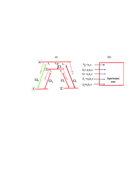
Figure 1: (a) Schematics of the Double Lambda Atomic system. (b) Doppler-broadened system

One of the modified media is the Left-handed medium which posses simultaneously negative electric permittivity and magnetic permeability pendry1996 ; pendry1998 ; pendry1999 . Earlier explored left-handed media were anisotropic in nature. Nevertheless, later with the use of new techniques isotropic left handed media were also realized shelby2001 ; shelbyrd2001 . Both the permittivity and permeability were required negative ($\epsilon,\mu<0$) for a negative refractive index with the magmatic dipole moments very smaller than the electric one. Nevertheless, due to the above rigorous condition, media with negative permeability in the optical frequencies domain met very rarely. Even with these complications, material media of negative refractive index based on EIT and photonic resonance were also studied.

Obviously, the quantum coherence and interference effect has remarkable impact on the speed of a probe pulse. Consequently, high degree control over the group velocity has been made possible both theocratically and experimentally. The detail study in this direction is very large. Nevertheless, some related works can be found in he1991 ; AK95 ; LV99 ; DD99 ; OS96 ; cg1970 ; scw1982 ; bs1985 ; Bs2005 ; yrc2002 ; bab2013 ; MM99 ; AK95 ; gs03 ; shang08 and in the references therein. Further, Moti and his co-worker have been presented an experimental demonstration for temporal cloaking while using the concepts of time-space duality between diffraction and dispersive broadening. Their experiment may be significant effort toward the development of complete spatio-temporal cloaks while using negative refractive indices Moti2012 . Glasser et al RYANT2012 used four-wave mixing in hot atomic vapors and experimentally measured multi-spacial-mode images with the use of negative group velocity. In this experiment the degree of temporal reshaping was quantified and increased with the an increase of the pulse-time-advancement. Furthermore, to impart the information of images in an optical pulse propagating through a region of anomalous dispersion may have a large number of potential applications while avoiding the pulse reshaping. Four-waves mixing in double-Lambda scheme of the Rubidium atom has also been shown to exhibit multi-spatial-mode entanglement vbmp2008 . Nevertheless, a system exhibiting less losses or gain may lead to an ideal multi-spatial-mode entanglement. The spatial properties of the multi-spatial-mode entanglement may also be precessed in the presence of fast light medium if the system is constrained to less losses or gains.

In this paper we investigate the effect of a chiral cold and hot medium of double Lambda type atoms on a propagating pulse. The chiral medium is a medium in which the electric polarization is coupled to the magnetic field component of the incident electromagnetic fields in free space while the magnetization is coupled to the incident electric field components. These mechanisms of the atom-field interaction ensures the proposed medium to posses the characteristics of negative refractive index even with no need of negative permittivity and permeability jbpendry2004 . In this connection, we select a chiral cold and hot atomic medium and investigate the effect of chirality on EIT and consequently on subluminal and superluminal behavior of the propagating pulse. Unlike the traditional degrading behavior of the Doppler broadened medium, here we explored contrastingly, an enhancement in the superluminal behavior of the propagating probe pulse for the hot chiral medium. Furthermore, we note that the nature of the propagation is different for suitably different set of parameters. Our explored undistorted retrieved pulse from a hot chiral medium delays significantly as compared with a cold chiral medium with a similar conditions. Nevertheless, the pulse advances enormously with a suitably different spectroscopic parameters. Evidently, the behavior of the propagating pulse is modified when the medium is reverted from Doppler broadened (hot) to the Doppler-free (cold) mode and vice versa. The group index of the medium, time delay/advance is also studied and analyzed explicitly.

We choose a four-level atomic system in Double-lambda configuration as shown in Fig. 1. The lower hyperfine ground levels $\left|1\right\rangle$ and $\left|2\right\rangle$ are coupled with the upper excited level $\left|4\right\rangle$, by a control field having Rabi frequency $\Omega_{2}$, and with a probe field having Rabi frequency $\Omega_{p}$, respectively. The excited hyperfine state $\left|3\right\rangle$ is coupled with the same lower ground levels by a magnetic field with the Rabi frequency $\Omega_{b}$, and a control field with the Rabi frequency $\Omega_{1}$, respectively. We also coupled the two excited hyperfine levels $\left|3\right\rangle$ and $\left|4\right\rangle$ by a microwave field with the Rabi frequency $\Omega_{3}$. Further, to keep the nature of interaction general we consider these fields detuned from their respective coupling energy levels and are defined as under: $\Delta_{1}=\omega_{13}-\omega_{1}$, $\Delta_{2}=\omega_{14}-\omega_{2}$ and $\Delta_{p}=\omega_{14}-\omega_{p}$, $\Delta_{b}=\omega_{13}-\omega_{b}$, $\Delta_{3}=\omega_{34}-\omega_{3}$. Next to drive the equations of motion and analyze optical response functions for the system, we proceed with the following interaction picture Hamiltonian in the dipole and rotating wave approximations as:

$$H(t) = -\frac{\hbar}{2}\Omega_{p}\exp[-i\Delta_{p}t]\left|1\right\rangle\left\langle 4\right|-\frac{\hbar}{2}\Omega_{b}\exp[-i\Delta_{b}t]\left|1\right\rangle\left\langle 3\right|$$ (1)

$$-\frac{\hbar}{2}\Omega_{1}[-i\Delta_{1}t]\left|2\right\rangle\left\langle 3\right|-\frac{\hbar}{2}\Omega_{2}\exp[-i\Delta_{2}t]\left|2\right\rangle\left\langle 4\right|$$

$$-\frac{\hbar}{2}\Omega_{3}\exp[-i\Delta_{2}t+i\varphi]\left|3\right\rangle\left\langle 4\right|+H.c.$$

The general form of density matrix equation is given by the following relation:

$$\frac{d\\ \rho_{t}}{dt}=\frac{-i}{\hbar}[\rho_{t},H_{t}]-\frac{1}{2}\Gamma_{ij}\sum(\sigma^{\dagger}\sigma\rho+\rho\sigma^{\dagger}\sigma-2\sigma\rho\sigma^{\dagger})$$ (2)

where $\sigma^{\dagger}$ is the raising operator and $\sigma$ is lowering operator for the four decays processes. Here, in the dynamical equation we use the transformation equation of fast varying transition matrix elements to the slowly varying transition matrix element through the $\rho_{ij}=\widetilde{\rho}_{ij}\exp[-i\Delta_{ij}]$, to remove the time dependent exponential factors. Finally, we obtained the three coupled dynamical equations for our system as:

$$\overset{\cdot}{\overset{\sim}{\rho}}_{14} = [i\Delta_{p}-\frac{1}{2}(\gamma_{1}+\gamma_{2})]\widetilde{\rho}_{14}+\frac{i}{2}\Omega_{p}(\widetilde{\rho}_{11}-\widetilde{\rho}_{44})$$ (3)

$$+\frac{i}{2}\Omega_{3}\exp[i\varphi]\widetilde{\rho}_{13}+\frac{i}{2}\Omega_{2}\widetilde{\rho}_{12}-\frac{i}{2}\Omega_{b}\widetilde{\rho}_{34},$$

$$\overset{\cdot}{\overset{\sim}{\rho}}_{13} = [i\Delta_{b}-\frac{1}{2}(\gamma_{1}+\gamma_{2})]\widetilde{\rho}_{13}+\frac{i}{2}\Omega_{b}\widetilde{\rho}_{11}+\frac{i}{2}\Omega_{1}\widetilde{\rho}_{12}$$ (4)

$$-\frac{i}{2}\Omega_{b}\widetilde{\rho}_{33}-\frac{i}{2}\Omega_{p}\widetilde{\rho}_{43}+\frac{i}{2}\Omega_{3}\exp[-i\varphi]\widetilde{\rho}_{14},$$

$$\overset{\cdot}{\overset{\sim}{\rho}}_{12} = [i(\Delta_{p}-\Delta_{2})-\frac{1}{2}(\gamma_{1}+\gamma_{2}+\gamma_{3}+\gamma_{4})]\widetilde{\rho}_{12}-\frac{i}{2}\Omega_{1}\widetilde{\rho}_{13}$$ (5)

$$+\frac{i}{2}\Omega_{2}\widetilde{\rho}_{14}-\frac{i}{2}\Omega_{b}\widetilde{\rho}_{32}-\frac{i}{2}\Omega_{p}\widetilde{\rho}_{42},$$

In the derivation of the above dynamical equation we considered $\Omega_{p}$, and $\Omega_{b}$ in the first order, while $\Omega_{1}$, $\Omega_{2}$ and $\Omega_{3}$ are assumed in all order of the perturbations. Next, we assume the atoms initially in the ground state $\left|1\right\rangle$. Therefore, the population initially in the other states is zero i.e., $\widetilde{\rho}_{11}=1$, $\widetilde{\rho}_{44}=\widetilde{\rho}_{34}=0$, $\widetilde{\rho}_{32}=\widetilde{\rho}_{33}=0$, $\widetilde{\rho}_{42}=\widetilde{\rho}_{43}=0$. Next, we assume the temperature of the medium hot and assume the system Doppler-broadened. To incorporate the broadening effect in the system we replaced the detuning parameters by: $\Delta_{1}=\Delta_{1}+\alpha_{1}k_{1}v$, $\Delta_{2}=\Delta_{2}+\alpha_{2}k_{2}v$, $\Delta_{b}=\Delta_{b}+\alpha_{3}k_{b}v$ $\Delta_{p}=\Delta_{p}+kv$. In the above replacement If we consider $\alpha_{i=1,2,3}=1$, then the coherent fields are co-propagating with the probe field while $\alpha_{i=1,2,3}=-1$ represent their corresponding counter propagation. Here $k_{1}$, $k_{2}$, $k_{3}$ ,$k_{p}$, $k_{b}$ are the wave vectors of coherent fields and the probes electric and magnetic fields. Nevertheless, we assumed $k_{1}=k_{2}=k_{3}=k_{b}=k_{p}=k$, in our analysis for a simplicity. To evaluate $\widetilde{\rho}_{14}^{(1)}$ and $\widetilde{\rho}_{13}^{(1)}$ in its steady state limit we used the following expression.

$$Y(t)=\int^{t}_{-\infty}e^{-M(t-t^{,})}Xdt^{,}=-M^{-1}X,$$ (6)

where $Y(t)$ and $X$ are column matrices while M is a 3x3 matrix. The solutions obtained are given bellow

$$\widetilde{\rho}_{14}^{(1)}=\Omega_{p}\beta_{EE}+\Omega_{b}\beta_{EB},$$ (7)

$$\widetilde{\rho}_{13}^{(1)}=\Omega_{p}\beta_{BE}+\Omega_{b}\beta_{BB},$$ (8)

where

$$\beta_{EB}=\beta_{BE}^{*}= \frac{-(i\Omega_{1}\Omega_{2}+2\Omega_{3}A_{3}\exp[i\varphi])}{2[\Omega_{1}\Omega_{2}\Omega_{2}\sin\varphi-\Omega^{2}_{1}A_{1}+\Omega^{2}_{2}A_{2}+(\Omega^{2}_{3}+4A_{1}A_{2})A_{3}]},$$ (9)

and

$$\beta_{EE,(BB)}= \frac{(-i)i(\Omega^{2}_{1}(+)-4A_{2(1)}A_{3})}{2[\Omega_{1}\Omega_{2}\Omega_{2}\sin\varphi-\Omega^{2}_{1}A_{1}+\Omega^{2}_{2}A_{2}+(\Omega^{2}_{3}+4A_{1}A_{2})A_{3}]},$$ (10)

while

$$A_{1}=[i(\Delta_{p}+kv)-\frac{1}{2}(\gamma_{1}+\gamma_{2})],$$ (11)

$$A_{3}=[i(\Delta_{b}+\alpha_{3}kv)-\frac{1}{2}(\gamma_{1}+\gamma_{2})],$$ (12)

and

$$A_{2}=[i(\Delta_{1}+\alpha_{1}kv-\Delta_{b}-\alpha_{3}kv)-\frac{1}{2}(\gamma_{1}+\gamma_{2}+\gamma_{3}+\gamma_{4})].$$ (13)

In Eqs. (7) and (8) $\beta_{EE}$ and $\beta_{BB}$, appear for electric and magnetic polarizabilities, while $\beta_{EB}$ and $\beta_{BE}$, represents the chirality coefficients. The electric polarization is defined by $P=N\sigma_{14}\rho_{14}$, and magnetization can be measured from $M=N\mu_{13}\rho_{13}$, where $\sigma_{14}$, is the electric and $\mu_{13}$, is the magnetic dipole moments and $N$, represents atomic number density. The Rabi frequencies are related to electric and magnetic fields through the relations, $\Omega_{p}=\sigma_{14}.E/\hbar$ and $\Omega_{b}=\mu_{13}.B/\hbar$, respectively. The electric and magnetic polarizations collectively is given by a simplified form as under

$$P,(M)=\frac{N\sigma^{2}_{14}\beta_{EE,(BB)}}{\hbar}E,(B)+\frac{N\sigma_{14}\mu_{13}\beta_{EB,(BE)}}{\hbar}B,(E),$$ (14)

where $B=\mu_{0}(H+M)$. Substituting the value of $B$ in magnetic polarization, and rearranging the equation we obtained the magnetization as:

$$M(kv)=\frac{N\mu_{0}\mu^{2}_{13}\beta_{BB}}{\hbar-N\mu_{0}\mu^{2}_{13}\beta_{BB}}H+\frac{N\mu_{13}\sigma_{14}\beta_{BE}}{\hbar-N\mu_{0}\mu^{2}_{13}\beta_{BB}}E$$ (15)

Substituting the value of $M$, and $B=\mu_{0}(H+M)$, in $P$, we obtained the expression for electric polarization as under

$$P(kv) = \frac{G+N\sigma^{2}_{14}\beta_{EE}(\hbar-N\mu_{0}\mu^{2}_{13}\beta_{BB})}{\hbar(\hbar-N\mu_{0}\mu^{2}_{13}\beta_{BB})}E$$ (16)

$$+\frac{N\sigma_{14}\mu_{0}\mu_{13}\beta_{EB}}{(\hbar-N\mu_{0}\mu^{2}_{13}\beta_{BB})}H,$$

$$G=N^{2}\sigma_{14}\mu_{0}\mu^{2}_{13}\beta_{BE}\beta_{EB}.$$

The susceptibility is a response function of the medium due to an applied electric field. The electric and magnetic polarizations in the form of chiral-based electric and magnetic susceptibility are defined by $P=\epsilon_{0}\chi_{e}E+\frac{\xi_{EH}}{c}H$ and $M=\frac{\xi_{HE}}{\mu_{0}c}E+\chi_{m}H$, respectively. These electric and magnetic susceptibilities for the hot atomic system is written as:

$$\chi_{e}(kv)= \frac{N^{2}\sigma_{14}\mu_{0}\mu^{2}_{13}\beta_{BE}\beta_{EB}+N\sigma^{2}_{14}\beta_{EE}(\hbar-N\mu_{0}\mu^{2}_{13}\beta_{BB})}{\epsilon_{0}\hbar(\hbar-N\mu_{0}\mu^{2}_{13}\beta_{BB})}$$ (17)

and

$$\chi_{m}(kv)=\frac{N\mu_{0}\mu^{2}_{13}\beta_{BB}}{\hbar-N\mu_{0}\mu^{2}_{13}\beta_{BB}},$$ (18)

respectively. The associated chiral coefficients are presented in the following single equation:

$$\xi_{EH,(HE)}(kv)=\frac{Nc\sigma_{14}\mu_{0}\mu_{13}\beta_{EB,(BE)}}{(\hbar-N\mu_{0}\mu^{2}_{13}\beta_{BB})}.$$ (19)

Here, the electric dipole moment is defined as $\sigma_{14}=\sqrt{3\gamma_{1}\epsilon_{0}\hbar c^{3}/2\omega^{3}_{14}}$. We select $v=0$ when the medium is cold and obviously the Doppler broadening effect can be minimized. The medium is then called as a cold chiral medium. Nevertheless, If a hot medium is considered, where the Doppler shift is dominant. we denote it as a hot chiral atomic medium. For cold atomic medium, we represent susceptibilities by $\chi_{e}$ and $\chi_{m}$, while for the chiral these are $\xi_{EH}$ and $\xi_{HE}$, respectively. These results are obtain from Eqs. (18)-(21], when one put $v=0$. The Doppler susceptibilities are the average of $\chi_{e}(kv)$, and $\chi_{m}(kv)$, over the Maxwellian distribution. The averaged electric and magnetic susceptibilities can be estimated separately from the following combined expression

$$\chi_{e,(m)}^{(d)}=\frac{1}{V_{D}\sqrt{\pi}}\int^{\infty}_{-\infty}\chi_{e,(m)}(kv)e^{-\frac{(kv)^{2}}{V^{2}_{D}}}d(kv)$$ (20)

where $V_{D}=\sqrt{K_{B}T\omega^{2}Mc^{2}}$, is the Doppler width. Here, $\chi_{e}^{(d)}$ and $\chi_{m}^{(d)}$ are the Doppler broadened electric and magnetic susceptibilities for hot atomic system. In the similar way we can estimate the chiral coefficient terms of the coupled electric -magnetic fields averaged over the Maxwellian distribution of the atomic velocity as

$$\xi_{EH,(HE)}^{(d)}=\frac{1}{V_{D}\sqrt{\pi}}\int^{\infty}_{-\infty}\xi_{EH}(kv)[\xi_{EH}(kv)]e^{-\frac{(kv)^{2}}{V^{2}_{D}}}d(kv)$$ (21)

We know that the refractive index of a medium is $n_{r}=\sqrt{\epsilon\mu}$, where $\epsilon=1+\chi_{e}$ and $\mu=1+\chi_{m}$. The terms $\xi_{EH}$ and $\xi_{HE}$ is the conurbation from chirality to the refractive index. The corresponding chiral dependent refractive then gets its shape as:

$$n_{r} = Re[((1+\chi_{e})(1+\chi_{m})-\frac{1}{4}(\xi_{EH}+\xi_{HE})^{2})^{1/2}$$ (22)

$$+\frac{i}{2}(\xi_{EH}-\xi_{HE})]$$

The group refractive index and Group velocity are also presented here as:

$$N_{g}=Re[n_{r}+(\omega_{14}-\Delta_{p})\frac{\partial n_{r}}{\partial\Delta_{p}}],$$ (23)

and

$$v_{g}=\frac{c}{Re[n_{r}+(\omega_{14}-\Delta_{p})\frac{\partial n_{r}}{\partial\Delta_{p}}]},$$ (24)

respectively. The corresponding time delay/advance is defined as $\tau_{d}=\frac{L(N_{g}-1)}{c}$. These are the main results which will be analyzed and discussed in details in the last section.

Further we used the transfer function for observation of out put pulse shape. The output pulse shape $E_{out}(\omega)$, after propagating through the medium can be related to the input pulse shape $E_{in}(\omega)$ by the expression $E_{out}(\omega)=H(\omega)E_{in}(\omega)$, where $H(\omega)=e^{-ik(\omega)L}$ is the transfer function for totally transmitting medium. we select a Gaussian input pulse of the form:

$$E_{in}(t)=\exp[-t^{2}/\tau^{2}_{0}]\exp[i(\omega_{0}+\delta)t],$$ (25)

where $\delta$, is the upshifted frequency from the empty cavity. The Fourier transforms of this function is then written by $E_{in}(\omega)=\frac{1}{\sqrt{2\pi}}\int^{\infty}_{-\infty}E_{in}(t)e^{i\omega t}dt$. The input signal is calculated as

$$E_{in}\left(\omega\right) = \tau_{0}/\sqrt{2}\exp\left[-\left(\omega-\omega_{0}-\delta\right)^{2}\tau^{2}._{0}/4\right]$$ (26)

The output $E_{out}(t)$ can be obtain from the input pulse by the convolution theorem as:

$$E_{out}(t)=\frac{1}{\sqrt{2\pi}}\int^{\infty}_{-\infty}E_{int}(\omega)H(\omega)e^{i\omega t}d\omega$$ (27)

For simplicity the output pulse shape is calculated in to the first order derivative of group index. It is reported as:

$$E_{out}(t) = \frac{\tau_{0}\sqrt{c}}{\sqrt{2iLcG_{vd}+c\tau^{2}_{0}}}\exp[\frac{[2i(Ln_{0}-ct)-\delta\tau^{2}_{0}c]^{2}}{4c(2iLcG_{vd}+c\tau^{2}_{0})}]$$ (28)

$$\times\exp[i(t-\frac{n_{0}L}{c})\omega_{0}-\frac{\delta^{2}\tau^{2}_{0}}{4}]:$$

The inverse fourier transform of $E_{out}(t)$ is $E_{out}(\omega)$ and is written by:

$$E_{out}(\omega) = \frac{\sqrt{2}\pi}{\Delta w}\exp[-\frac{Q_{1}^{2}}{4c(2iLcG_{vd}+\frac{4c\pi^{2}}{(\Delta w)^{2}})}]$$ (29)

$$\times\exp[\frac{1}{4}(-\frac{4\pi^{2}\delta^{2}}{\Delta w}+Q_{2}-\frac{4i\omega_{0}Ln_{0}}{c})],$$

where

$$Q_{1}=2iL(\omega-\omega_{0})cG_{vd}+\frac{4c\pi^{2}(\omega-\omega_{0}-\delta)}{(\Delta w)^{2}}+2iLn_{0}$$ (30)

and

$$Q_{2}=\frac{[\frac{4c\pi^{2}\delta}{(\Delta w)^{2}}-2iLn_{0}]^{2}}{c(2iLcG_{vd}+\frac{4c\pi^{2}}{(\Delta w)^{2}})}.$$ (31)

In Eqs. (32)-(35), $n_{0}=\lim_{\omega\longrightarrow\omega_{0}}N_{g}$, $G_{vd}=\lim_{\omega\longrightarrow\omega_{0}}\frac{\partial N_{g}}{c\partial\omega}$ while $\tau_{0}$ appeared for the input pulse width in the time domain. Also, $G_{vd}$ is the group velocity dispersion and $\omega_{0}$ is the central frequency of the pulse. Furthermore, the resonances appears at the location $\omega_{0}=\omega_{14}$. It is the frequency of the pulse at which the delay or advancement time is maximum and the distortion is minimum.

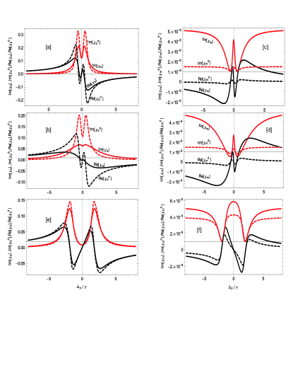
Figure 2: Electric and magnetic Real as well as imaginary susceptibilities vs probe detuning $\Delta_{p}/\gamma$, such that $\gamma=1GHz$, $\gamma_{1}=\gamma_{1}=\gamma_{3}=\gamma_{4}=0.1\gamma$, $\Delta_{1}=0\gamma$, $\Delta_{2}=0\gamma$, $\Delta_{b}=0\gamma$, $\Omega_{1}=0.1\gamma$, $\Omega_{2}=1\gamma$, $V_{D}=0.5\gamma$, $\alpha_{i}=\pm 1$, $\mu_{13}=0.000053\sigma_{14}ms^{-1}$, $\lambda=1nm$[a,c] $\Omega_{3}=0.7\gamma$[b,d] $\Omega_{3}=1\gamma$, $\varphi=\pi/2$ [e,f]$\Omega_{2}=4\gamma$, $\Omega_{3}=0.7\gamma$, $V_{D}=0.1\gamma$

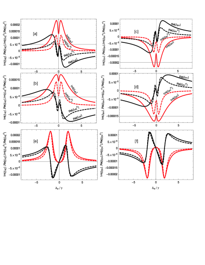
Figure 3: Real and imaginary parts of chiralities vs probe detuning $\Delta_{p}/\gamma$, such that $\gamma=1GHz$, $\gamma_{1}=\gamma_{1}=\gamma_{3}=\gamma_{4}=0.1\gamma$, $\Delta_{1}=0\gamma$, $\Delta_{2}=0\gamma$, $\Delta_{b}=0\gamma$, $\Omega_{1}=0.1\gamma$, $\Omega_{2}=1\gamma$, $V_{D}=0.5\gamma$, $\alpha_{i}=\pm 1$, $\mu_{13}=0.000053\sigma_{14}ms^{-1}$, $\lambda=1nm$[a,c] $\Omega_{3}=0.7\gamma$[b,d] $\Omega_{3}=1\gamma$, $\varphi=\pi/2$ [e,f]$\Omega_{2}=4\gamma$, $\Omega_{3}=0.7\gamma$, $V_{D}=0.1\gamma$

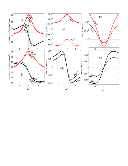
Figure 4: Electric and magnetic Real as well as imaginary susceptibilities vs probe detuning $\Delta_{p}/\gamma$, such that $\gamma=1GHz$, $\gamma_{1}=\gamma_{1}=\gamma_{3}=\gamma_{4}=2\gamma$, $\Delta_{1}=0\gamma$, $\Delta_{2}=0\gamma$, $\Delta_{b}=0\gamma$, $\Omega_{1}=2\gamma$, $\Omega_{2}=2\gamma$, $V_{D}=1.5\gamma$, $\alpha_{i}=\pm 1$, $\mu_{13}=0.000053\sigma_{14}ms^{-1}$, $\lambda=1nm$[a,c] $\Omega_{3}=1.5\gamma$[b,d] $\Omega_{3}=5\gamma$, $\varphi=\pi/2$

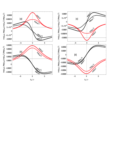
Figure 5: Real and imaginary parts of chirality vs probe detuning $\Delta_{p}/\gamma$, such that $\gamma=1GHz$, $\gamma_{1}=\gamma_{1}=\gamma_{3}=\gamma_{4}=2\gamma$, $\Delta_{1}=0\gamma$, $\Delta_{2}=0\gamma$, $\Delta_{b}=0\gamma$, $\Omega_{1}=2\gamma$, $\Omega_{2}=2\gamma$, $V_{D}=1.5\gamma$, $\alpha_{i}=\pm 1$, $\mu_{13}=0.000053\sigma_{14}ms^{-1}$, $\lambda=1nm$[a,c] $\Omega_{3}=1.5\gamma$[b,d] $\Omega_{3}=5\gamma$, $\varphi=\pi/2$

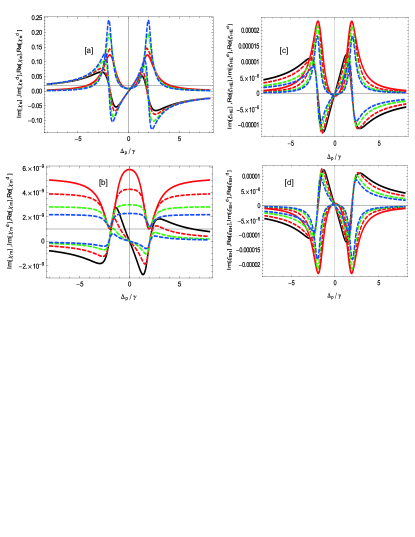
Figure 6: Electric and magnetic Real as well as imaginary susceptibilities vs probe detuning $\Delta_{p}/\gamma$, such that $\gamma=1GHz$, $\gamma_{1}=\gamma_{1}=\gamma_{3}=\gamma_{4}=0.1\gamma$, $\Delta_{1}=0\gamma$, $\Delta_{2}=0\gamma$, $\Delta_{b}=0\gamma$, $\Omega_{1}=0.1\gamma$, $\alpha_{i}=\pm 1$, $\mu_{13}=0.000053\sigma_{14}ms^{-1}$, $\lambda=1nm$, $\varphi=\pi/2$, $\Omega_{2}=4\gamma$, $\Omega_{3}=0.7\gamma$, $V_{D}=0\gamma$(solid), $0.1\gamma$(red dashed), $0.2\gamma$(green dashed), $0.3\gamma$(blue dashed)

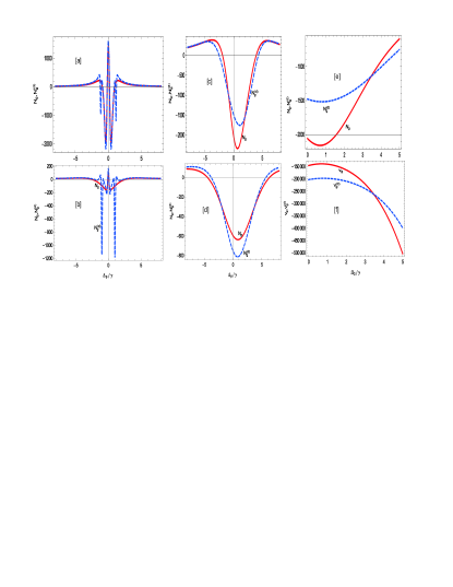
Figure 7: [a,b,c,d] Group index vers probe detuning $\Delta_{p}/\gamma$, such that $\gamma=1GHz$, $\gamma_{1}=\gamma_{1}=\gamma_{3}=\gamma_{4}=2\gamma$, $\Delta_{1}=0\gamma$, $\Delta_{2}=0\gamma$, $\Delta_{b}=0\gamma$, $\Omega_{1}=2\gamma$, $\Omega_{2}=2\gamma$, $V_{D}=1.5\gamma$, $\alpha_{i}=\pm 1$, $\mu_{13}=0.000053\sigma_{14}ms^{-1}$, $\lambda=1nm$, $\omega_{14}=10^{4}\gamma$,$L=6cm$[a,c] $\Omega_{3}=1.5\gamma$[b,d] $\Omega_{3}=5\gamma$, $\varphi=\pi/2$[e,f] Group index and group velocity vers $\Omega_{3}/\gamma$, using the same parameters but $\Delta_{p}=0\gamma$

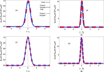
Figure 8: [a,b]The normalized Gaussian pulse intensity of input and outputs at the parameters given Fig2, Vs $\frac{t}{\tau_{0}}$ and $\frac{\omega-\omega_{0}}{\Delta w}$, $\delta=2GHz$, $\tau_{0}=5.50ns$, $\Delta w=2\pi/\tau_{0}$, $c=3\times 10^{8}m/s$, $L=0.06m$, $n_{0}=1415.65$, $n^{d}_{0}=1618.15$, $G_{vd}=759.44/c$, $G^{d}_{vd}=18.92/c$, $\omega_{0}=\omega_{14}=10^{4}\gamma$[c,d]The normalized Gaussian pulse intensity of input and outputs at the parameters given Fig4, Vs $\frac{t}{\tau_{0}}$ and $\frac{\omega-\omega_{0}}{\Delta w}$, $n_{0}=-2023.81$, $n^{d}_{0}=-1487.22$, $G_{vd}=-9006.67/c$, $G^{d}_{vd}=-344.57/c$

We explain our main results of the Eqs. (18)-(21)] associated with the Real and imaginary parts of electric and, magnetic susceptibilities and their corresponding chiralities, for both Doppler broadened and Doppler-free systems. The discussion is then extended to group index, time delay and pulse shape distortion using their analytical expressions presented in the earlier text. In Fig. 2, the plots are traced for electric and magnetic susceptibilities for some spectroscopic parameters. Obviously the behavior of electric susceptibility is in contrast with The electric and magnetic susceptibility. Therefore, the dispersion associated with electric susceptibility is contrastingly opposite to the anomalous dispersion of the magnetic one with a less absorption in comparison. Evidently, the absorption profile enhances with the hot medium as compared with the cold one.

Intriguingly, the behavior of chirality in case of electric field coupling is the mirror inversion as compared with the behavior of magnetic coupling along with an enhanced profile for Doppler-free system over the Doppler-broadened. Nevertheless, the intensity of the microwave field generates incoherence processes and disturbs the interference mechanism of the system. The light propagation in former corresponds to slow while later it corresponds to fast light. Amazingly, in the hot medium the Doppler shift develops coherence and the the dip between the two peak absorption lines becomes more obvious. Consequently, unlike in the traditional superluminality where the Doppler shift degrade the super luminal fast light, here it enhances significantly.

Different spectral behaviors are observed, when there is no Doppler broadening (cold system) as well as, when there is Doppler broadening (hot system) in the system. The solid line is for Doppler free susceptibility and the dashed line is for Doppler broadened susceptibility. The electric and magnetic susceptibilities have opposite absorption and dispersion behavior as shown in Fig .2[a-d]. The absorption at resonance $\Delta_{p}=0$, is reduced in the electric susceptibility, while there is increase in the magnetic susceptibility. The slope of dispersion is normal in the electric susceptibility, while anomalous in the magnetic susceptibility. Nevertheless, the magnetic effect on absorption and dispersion is very small as compared with the electric effect on absorption and dispersion. Further, with the control field $\Omega_{3}=0.7\gamma$, the absorption at resonance in both the cases (cold/hot) are $0.2au$. Nevertheless, the absorption reduces in the Doppler free medium to $0.05au$ when the control field intensity is increased to $\Omega_{3}=1\gamma$ and have small gaps in both the absorption and dispersion. The modification at $\Delta_{p}=0$ of slow light propagation at the resonance point from cold to hot atomic medium is also obvious. Further, in Fig .3[a-d] the real and imaginary parts of chiralities $\xi_{HE}$ and $\xi_{EH}$ under similar condition of Fig 2 are traced which also show opposite behavior for the real and imaginary parts, respectively.

The real and imaginary parts of chirality $\xi_{HE}$ ($\xi_{EH}$) shows similarity with electric (magmatic) susceptibility in real as well as imaginary parts of the susceptibility with inverted behaviors from cold to hot medium at resonance $\Delta_{p}=0$ as shown in Fig 2[c,d] and Fig 3[a,b]. Consequently, their dynamical characteristics have contrast behavior for the dispersion and absorption for the two cases, respectively. [see Fig 2[a,b] and Fig 3[c,d]]. The dominant chiral effect on magnetic susceptibility is also obvious as compared with the electric one.

Curiositly, controlling the intensity associated with $\Omega_{2}$, the absorption in the electric susceptibility and chirality $\xi_{HE}$ becomes vanished while it is increased for the magnetic susceptibility and chirality $\xi_{EH}$. The symmetries in $\chi_{e}$ and $\xi_{HE}$, and in $\chi_{m}$ and $\xi_{EH}$ is ideal. These interesting results are observed at the parameters $\gamma_{i=1,2,3,4}=0.1\gamma$, $\Omega_{1}=0.1\gamma$, $\Omega_{2}=4\gamma$, $V_{D}=0.1\gamma$ and $\Omega_{3}=0.7\gamma$, $\alpha_{i}=\pm 1$ and $\varphi=\pi/2$, as shown in Fig .2[e,f] and Fig .3[e,f].

In Figs .(4)-(5) the real and imaginary parts of chiralities $\xi_{EH}$ and $\xi_{EH}$, are shown with the same parameters. The absorption of cold medium is less (large) than the absorption of hot medium at low (large) intensity of the control field $\Omega_{3}=1.5\gamma$, at the resonance point. The real and imaginary parts of the chirality $\xi_{HE}$ have similar spectral behavior as compared with $\chi_{e}$ for low intensity of the control field for both the cold and hot atomic medium. Nevertheless, for high intensity of the control field the spectral behaviors are inverted for both the cold and hot atomic medium as shown in Fig 4[a,b] and Fig 5[a,b]. Furthermore, similar characteristics is also true for $\xi_{EH}$ for its real and imaginary parts of the magnetic when the the intensity of the control field is high as shown in Fig 4[d] and Fig 5[d]. In Fig .6 the electric and magnetic susceptibilities and the chiralities are traced with the Doppler widths, a parameter controllable with temperature of the medium. A very dominant response is seen about the time delay and advance when the Doppler width is increased stepwise. Consequently, going cold chiral medium to a hot chiral medium the behavior of the system can be reverted.

The group index and time delay/advancement for the parameters of Fig .2 is shown in Fig. 7. At the resonance point $\Delta_{p}/\gamma=0$ sharp positive peaks of group indices and times delays/advancement are observed. When the intensity of the control field $\Omega_{3}$ is $0.5\gamma$, the value of group index for cold medium is $N_{g}=1415.65$ and the value of group index for hot medium is $N^{(d)}_{g}=1618.15$. The corresponding group delays are $t_{d}=121ns$ and $t^{(d)}_{d}=917ns$. If the intensity of control field $\Omega_{3}$ is increased from $0.7\gamma$ to $1\gamma$. Then the group index are $N_{g}=110.96$ and $N^{(d)}_{g}=164.013$, while delays in times are $t_{d}=219ns$ and $t^{(d)}_{d}=997ns$, respectively. Correspondingly, the group velocities vary from $v_{g}=c/1415.65$ to $v_{g}=c/110.96$ and $v^{(d)}_{g}=c/1618.15$ to $v^{(d)}_{g}=c/164.013$. The above results are spatially important to the preservation of two light pulses. When two light pulses reach at same times to the instrument which store its information. The instrument stored the information of one of the pulse and lost the information of the other pulse. There delays in times recovered this difficulty and the information of both the pulses will be preserved. In Fig. 7 (c,d), for $\Delta_{p}=0\gamma$, the values of group indices are $N_{g}=-2023.81$ and $N^{(d)}_{g}=-1487.22$ at the intensity of the control field $\Omega_{3}=1.5\gamma$. The corresponding advance times are $t_{ad}=-404ns$ and $t^{(d)}_{ad}=-297ns$. In this case the cold medium is more superluminal, and the advance time is larger then the hot medium by $107ns$. When the intensity of the control field is increase from $1.5\gamma$ to $5\gamma$, the group index of the cold medium is $N_{g}=-595.818$, while the group index of the hot medium is $N^{(d)}_{g}=-751.666$. The corresponding advance times are then $t_{ad}=-119.36s$ and $t^{(d)}_{ad}=-150.53ns$. The advance time difference is $31.17ns$. In this case the Doppler broadened medium is more superluminal than the Doppler free medium.

In the previous related studies, it has been observed that the Doppler broadened medium is less superluminal, than a Doppler free medium. Here a chiral medium shows contrastingly different behavior, that it may enhance superluminality at certain conditions of the coherent control field shown in Fig 7[d]. This fact is more clearly observed in the Fig 7[e,f]. It is clear from these plots that below the intensity of the control field $\Omega_{3}=3.6\gamma$, the group index of cold chiral medium is more negative with a larger group velocity as compared with the hot chiral medium. Therefore the chiral cold medium is more superluminal than the chiral hot medium below the intensity of control field of $3.6\gamma$. Nevertheless, for $\Omega_{3}>3.6\gamma$, the group index of the chiral hot medium is more negative and larger negative group velocity as compared to the chiral cold medium, Hence chiral hot medium is more superluminal above the intensity of the control field of $3.6\gamma$. Furthermore, at high intensity of the control field the group index and group velocity becomes saturated (not shown).

Fig .8 shows Gaussian pulse shapes of input and output of the chiral medium. All the pulses are the same shapes for cold and hot medium, if the coherent fields counter propagate to the probe field or co-propagate to the probe field up to first order group velocity dispersion. The pulses are fully distortion-less to the first order group index derivative with respect to angular frequency. However if one counts higher order derivative then the pulse is slowly distorted.

In conclusion, we study Chiral Based Electromagnetically Induced Transparency (CBEIT) of a light pulse and its associated subluminal and superluminal behavior through a cold and a hot medium of 4-level double-Lambda type atomic system. The dynamical behavior of this chiral based system is temperature dependent. The magnetic field based chirality and dispersion is always opposite as compared with the electric field ones. Contrastingly, the response of the chiral effect along with the incoherence Doppler broadening mechanism enhances the superluminal behavior as compared with its traditional degrading effect. Nevertheless, the intensity of a coupled microwave field destroys the coherence of the medium and degrade superluminality and subluminality of the sysmtem. The undistorted retrieved pulse from a hot chiral medium delays by $896ns$ than from a cold chiral medium under same set of parameters. Nevertheless, it advances by $-31ns$ in the cold chiral medium when a suitably different spectroscopic parameters are selected. The corresponding group index of the medium and the time delay/advance, are studied and analyzed explicitly [Note: A revise version is under preparation

References

(1)M. Fleischhauer, A. Imamoglu and J. P. Marangos, Rev. Mod. Phys. 77, 633 (2005).
(2) M. D. Lukin and A. Imamoglu, Nature, 413, 273 (2001).
(3)Pendry, J. B, A. J. Holden, W. J. Stewart, and I. Youngs,
, Phys. Rev. Lett. 76, 4773-4776, (1996).
(4)Pendry, J. B., A. J. Holden, D. J. Robbins, and W. J. Stewart,
J. Phys.Condens. Matter 10, 4785-4809, (1998).
(5)Pendry, J. B., A. J. Holden, D. J. Robbins, and W. J. Stewart,
Microwave Theory Tech. 47, 2075-2084, (1999).
(6)Shelby, R. A, D. R. Smith, and S. Schultz, Science, 292,
77-79, (2001).
(7)Shelby, R. A, D. R. Smith, S. C. Nemat-Nasser, and S. Schultz,
Appl. Phys. Lett,78, 489-491,
(2001).
(8) Koschny, T. L. Zhang, and C. M.
Soukoulis, Phys. Rev. B, 71, 121103(2005).
(9)Guney, D. O., T. Koschny, and C. M. Soukoulis, Opt. Express, 18, 12348-12353, (2010).
(10) N. Engheta, Propag. Lett. 1, 10-13, (2002).
(11)Shen, L., S. He, and S. Xiao, Phys. Rev. B, 69, 115111, (2004).
(12)Schurig, D., J. J. Mock, B. J. Justice, S. A. Cummer, J. B.
Pendry, A. F. Starr, and D. R. Smith,Science 314,
977-980, (2006).
(13)J. B. Pendry, Phys. Rev. Lett. 85, 3966 (2000).
(14)J. B. Pendry, Science 306, 1353 (2004).
(15)R. W. Boyd and D. J. Gauthier, Science 326, 1074-1077 (2009).
(16)K. J. Boller, A. Imamoglu, and S. E. Harris, Phys. Rev. Lett. 66,
2593(1991).
(17)A. Kasapi, M. Jain, G. Y. Yin, and S. E. Harris, Phys. Rev.
Lett. 74, 2447 (1995).
(18) L.V. Hau, S. E. Harris, Z. Dutton and C.H. Behroozi, Nature
(London) 397, 594 (1999 ).
(19) D.Budker, D. F. Kimball, S. M. Rochester, and V. V. Yashchuk, Phys.
Rev. Lett. 83, 1767 (1999).
(20) M. M. Kash, Scully, Phys. Rev. Lett. 82, 5229 (1999).
(21)O. Schmidt, R. Wynands, Z. Hussein, and
D. Meschede, Phys. Rev. A 53, R27 (1996).
(22) C. Garrett
and D. McCumber, Phys. Rev. A 1, 305 313 (1970).
(23)S. Chu and S. Wong, Phys. Rev. Lett. 48, 738 741 (1982).
(24) B. Segard and B.
Macke, Phys. Lett. 109, 213 216 (1985).
(25) B. Segard, B. Macke, and F.
Wielonsky, Phys. Rev. E 72, 035601 (2005).
(26) R. Y. Chiao and P. W. Milonni, Fast light, slow
light, Opt. Photon. News 13, 26 30 (2002). R. J. McLean,
Fast light in atomic media, J. Opt. 12,104001(2010).
(27)Bakht Amin Bacha, Iftikhar Ahmad, Arif Ullah and Hazrat
Ali,phys,Scr,88,045402(2013).
(28)G.S.Agarwal and T.N Dey, phys Rev. A 68, 063816(2003).