Combinatorial level densities by the real-time method

Abstract

Levels densities of independent-particle Hamiltonians can be calculated easily by using the real-time representation of the evolution operator together with the fast Fourier transform. We describe the method and implement it with a set of Python programs. Examples are provided for the total and partial levels densities of a heavy deformed nucleus (¹⁶⁴Dy). The partial level densities that may be calculated are the projected ones on neutron number, proton number, azimuthal angular momentum, and parity.

I introduction

Knowledge of nuclear level densities is important in nuclear reactions and decays, particularly for heavy nuclei. The starting point in the theory of level densities is the independent nucleon model, either from a shell model or a mean-field approximation. A quantitative theory requires a careful treatment of the interactions beyond mean field , but it is useful to have the independent particle level densities to build from. In principle that theory is very simple, needed only the single-particle energies to calculate the excitations. Even so, the computational problem remains nontrivial. The two well-known methods for treating it are the statistical approach using the partition function, and the combinatorial approach which individual particle-hole excitations are counted. The statistical approach via the partition function has two drawbacks. One is that the calculated partition function must be transformed to an actual level density by using the saddle-point approximation. This is accurate when the level density is high but is unsatisfactory as a complete solution. The other drawback is that partial level densities (mostly associated with conserved quantum numbers) may be awkward to extract. The combinatorial approach does not require that the level density be high, but it can also be awkward for writing codes when it depends on many quantum numbers that are to be exhibited explicitly in partial level densities. Here we shall show that the coding becomes quite simple using a real-time formulation of the problem and the Fast Fourier Transform (FFT). The one-dimensional FFT was first used to calculate level densities by Berger and Martinot be74 . However, for calculating partial level densities the formulation using the trace of the real-time Green’s function is more transparent and can be easily implemented by the multidimensional FFT. The codes to perform the calculations under different conditions are described in the appendix and are available for download.

II Real-time method

To derive the equations of the real-time method, let us consider a Fock space of $N_{p}$ orbitals with the Hamiltonian

$$\hat{H}=\sum_{i}^{N_{p}}\varepsilon_{i}a^{\dagger}_{i}a_{i}$$ (1)

where $\varepsilon_{i}$ are the single-particle energies of the orbitals. The total level density $\rho(E)$ is defined as

$$\rho(E)={\rm Tr}\left(\delta(\hat{H}-E)\right)$$ (2)

Here the trace runs over all states of the many-particle Fock space, i.e. with any number of particles in the space. Next, the $\delta$-function is represented by the Fourier transform

$$\delta(\hat{H}-E)={1\over 2\pi}\int_{-\infty}^{\infty}dt\,e^{iEt}e^{-i\hat{H}t}.$$ (3)

The trace of the operator in this equation is easy to evaluate due to the independent-particle character of the Hamiltonian. It is

$$G(t)\equiv{\rm Tr}\left(e^{-i\hat{H}t}\right)=\prod_{i}^{N_{p}}(1+e^{-i\varepsilon_{i}t}).$$ (4)

In practice, the computation is carried out by building a table of $G$ as a function of $t$ and then applying the Fourier transform by the FFT algorithm. Specifically, we apply the discrete FFT with time points $t_{i}$ as

$$\tilde{G}(E_{i})={\tt FFT}\,(G(2\pi t_{i}))$$ (5)

with $t_{i}$ forming a mesh with $N_{t}$ points separated by a fixed interval $\Delta t$. The result is $\tilde{G}$, an array with the elements giving the number of levels in an energy interval $\Delta E=1/\Delta t$ around the point $E_{i}$,

$$\tilde{G}(E_{i})=\int_{E_{i}}^{E_{i}+\Delta E}dE\,\rho(E)$$ (6)

To make the results completely transparent, it is helpful to discretize the single-particle energy spectrum with the same $\Delta E$. Provided the discretization in $t$ is sufficiently fine, the output of the FFT will be an integer in each energy bin.

We have coded Eq. (5) and Eq. (8,9) below for the total level density partial level densities in rt_levels3.py. The program is described in the Appendix and available for download. To illustrate its use, we calculate the neutron level density of the heavy deformed nucleus ¹⁶⁴Dy, taking the single-energies from the Hartree-Fock spectrum calculated with the Gogny D1S interaction. The single-particle space has been truncated to $N_{p}=40$ orbitals, taking the orbitals of the ¹⁶⁴Dy ground state closest to the Fermi level. The excitation energies in that space range from zero to $~{}120$ MeV, and the total number of states is $2^{40}=1.1\times 10^{12}$. The energy binning is taken as $\Delta E=0.2$ MeV. This implies that the FFT must be carried out with at least $120/0.2\sim 600$ time points. The resulting total level density is shown in Fig. 1 as the open circles.

Figure 1: Level densities for neutron levels in ¹⁶⁴Dy. Open circles are the total level densities. Black squares are projected onto states with equal numbers of particles and holes. Black circles are further projected onto states with $J_{z}=0$. The total and number-projected densities are binned with $\Delta E=0.2$ MeV bins; the $J_{z}$-projected densities are with $0.5$ MeV bins.

In practical applications we often would like level densities projected onto conserved quantum numbers. If the quantum numbers are additive, the projections can also be conveniently carried out by Fourier transform. For example, number projection is performed by introducing a second $\delta$-function in the trace formula,

$$\delta(\hat{N}-N)={1\over 2\pi}\int_{\infty}^{\infty}d\phi_{N}\,e^{i\hat{N}\phi_{N}}e^{-iN\phi_{N}}$$ (7)

where $\phi_{N}$ is a gauge angle. As before, the integral is evaluated as a discrete Fourier transform. This method for number projection is in common use, eg. in the shell-model Monte Carlo treatment of level densitiesor94 and in the extended Hartree-Fock-Bogoliubov theory of ground state energiesan01 . The program rt_levels3.py also includes the coding for the needed two-dimensional FFT, which we write as

$$\tilde{G}(E_{i},N)={\tt FFT2}\,(G(2\pi t_{i},2\pi\phi_{k}))$$ (8)

The discretization in gauge angle $\phi_{k}$ require at least as many angles as there are in the range of $N$ values in the output. This calculation is illustrated by the black squares in Fig. 1. The single-particle spectrum is the same as in the previous example; one sees that the projected level density is as much as an order of magnitude smaller.

The same technique can be used for any other additive quantum number. Besides particle number, we would like to project on $J_{z}$, the $z$-component of angular momentum. If the nuclear field is axially symmetric, the orbitals have a well-defined $J_{z}$ quantum number and an additional variable can be added to $G$ corresponding to rotation angles $\phi_{z}$ about the $z$-axis. The required three-dimensional Fourier transform is also coded in rt_levels3.py. We write it as

$$\tilde{G}(E_{i},N,J_{z})={\tt FFT3}\,(G(2\pi t_{i},2\pi\phi_{k},2\pi\phi_{z})).$$ (9)

The result for the combined $N$- and $J_{z}$-projection of the neutron level density in ¹⁶⁴Dy is shown in Fig. 1 as the black circles.

One can apply the same method to the parity operator. Since there are only two possible parities, it is sufficient to take only two angles $\phi=0$ and $\phi=\pi$ in constructing the $G$ array. The code rt_levels3.py has the flexibility to project on a fixed parity as well as carrying out the $N,Z,J_{z}$ projections at the same time.

One should be aware of two computational issues associated with the real-time method. First, roundoff error will be come severe if the size of the many-body space $2^{N_{p}}$ exceeds the number of bits in the floating point arithmetic. The examples in the Fig. 1 and Fig. 2 below have $N_{p}=40$, well below the 56 mantissa bits of the double precision arithmetic in the FFT program library calls. Second, the method is only fast if the number of simultaneous projections is limited. The running time on a laptop is of the order of seconds or minutes for the one- and the two-dimensional Fourier transforms. The three-dimensional transformation is on the scale of an hour, but higher order transforms would be quite time-consuming. We describe in the next section an approximate treatment of projections that might be preferable in those cases.

III Combining combinatorics with statistics

The most complete decomposition we can envisage here is to project on proton number $Z$, neutron number $N$, azimuthal quantum number $J_{z}$, and parity $P$. As discussed earlier, parity is easy to include. But the 4-dimensional array and Fourier transformed needed to do the $(N,Z,J_{z})$ projection is beyond the scope of laptop computation. Fortunately, the central limit theorem allows one to estimate the projections at a factor of 2 in cost for each projection.

We illustrate first with a single projection, for example, neutron number $N$. The one-dimensional FFT is carried out in the time-energy domain with two values of the neutron gauge angle, $\phi_{n}=0,\Delta\phi$. The angle $\Delta\phi$ is chosen to be small enough so that a power series expansion of $\tilde{G}$ in that variable is permitted. Then we can extract the first and second moments of $\hat{N}$ for each bin in $\tilde{G}(E)$. Call the total number of states in the bin $M_{E}$,

$$M_{E}=\tilde{G}(E,\phi=0).$$ (10)

The average number of particles and holes in those $M_{E}$ states is calculated as

$$N_{1}=\langle\hat{N}\rangle_{E}\approx{{\rm Im}\,\tilde{G}(E,\Delta\phi)\over M_{E}\Delta\phi}.$$ (11)

The mean square number of particles and holes is calculated as

$$N_{2}=\langle\hat{N}\hat{N}\rangle_{E}\approx{2\over\Delta\phi^{2}}\left(1-{{\rm Re}\tilde{G}(E,\Delta\phi)\over M_{E}}\right).$$ (12)

Now treat $N$ as a continuous variable and assume that the distribution in $N$ is Gaussian, with the same moments $N_{1}$ and $N_{2}$. This gives

$$P(N)={M_{E}\over\sigma\sqrt{2\pi}}\exp\left(-{(N-N_{1})^{2}\over 2\sigma^{2}}\right),$$ (13)

where

$$\sigma^{2}=N_{2}-N_{1}^{2}.$$ (14)

The program rt_levelsNP.py estimates the $N,Z$ and $K$ projections using Eqs. (7-10) assuming there are no correlations between the three variances except for one. Namely, the number parities of $2K$ and $N+Z$ are always equal, eg. $2K$ is even if $N+Z$ is even. So half the of entries in a table of level densities are zero, and the nonzero ones are on the average twice as large. Fig. 2 shows the calculated levels densities of ¹⁶⁴Dy using rt_levelsNP.py. One sees that the three-fold projection has a very strong effect on the level density, reducing it by more than two orders of magnitude in the 5-10 MeV range of excitation energies.

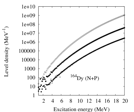
Figure 2: Level densities for ¹⁶⁴Dy including both neutron and proton excitations in a single-particle space totaling 40 orbitals. Open circles are the total level densities. Black squares are projected onto $\Delta N=0$ and $\Delta Z=0$ with respect to the zero-particle zero-hole ground state, using the approximate projection by Eq. 9. Black circles are further projected onto states with $J_{z}=0$ with the same method. Also shown with triangles is the exact projection calculated combining neutron and proton densities from Eq. (9).

Also in Fig. 2 we show the exact three-fold projected densities calculated by folding the neutron and proton level densities obtained from three-dimensional Fourier transforms. The results are indistinguishable for energies over 6 MeV. The program foldNP.py to carry out the folding is also included in the package of codes provided with this article.

Appendix

The examples in the text were computed with the programs rt_levels3.py, rt_levelsNP.py, and foldNP.py. A tar file of the three programs together with input data going with Figs. 1 and 2 is available on the website of one of the authors, www.phys.washington.edu/users/bertsch/computer.html under “Level Densities”. They are written in the Python programming language and require the numpy library to run. The programs have been tested with version 2.7.3 of Python and 1.6.1 of numpy.

The code for rt_levelsNP.py is reproduced below.

#  rt_levelsNP.py calculates level densities by 1D Fourier transform
# with neutrons and protons together; N,Z, and K projections are
# calculating assuming that the distributions are Gaussian.
import sys
import math as m
import numpy as np
import numpy.fft as fft

lines = open(sys.argv[1]).readlines()
datafile = lines[0].split()[0]
ss = lines[1].split()
Nt = int(ss[0])
Nphi,Zphi,Kphi = map(float,ss[1:4])
DeltaE = float(lines[2].split()[0])
lines = open(datafile).readlines()
Nnp = len(lines) -2
lines= lines[1:]
print ’Nt, Nnp, DeltaE’,Nt, Nnp,DeltaE
print ’phiN,phiZ,phiK’, Nphi,Zphi,Kphi
Qvals = []
Evals = np.array([0.0]*Nnp)
etot = 0.0
tau_z = 1
i = 0
for line in lines:
   ss = line.split()
   if len(ss) != 4:
      tau_z = -1
   else:
     K,P,B = map(int,ss[:3])
     if P == 1:  Pex = 0.0;
     if P == -1:  Pex = 1.0
     Qvals.append((K,Pex,B,tau_z))     # K,P,B,tau_z
     E = round(float(ss[3])/DeltaE+1.0e-4)
     Evals[i]= E
     etot += E
     i += 1
print ’DeltaE,etot’, DeltaE,etot

# set up the gauged Green’s function
ggauged = np.array([[0.0j]*Nt]*4)

Nphase=np.array([0.0]*Nnp)
Zphase=np.array([0.0]*Nnp)
Kphase=np.array([0.0]*Nnp)
nophase = np.array([0.0]*Nnp)
for ip in range(Nnp):
   K,Pex,B,tau_z = Qvals[ip]
   if tau_z == 1:
     Nphase[ip] = Nphi*B
   else:
     Zphase[ip] = Zphi*B
   Kphase[ip] = Kphi*K
print

# compute G(t,phi)

G = np.array([0.0j]*Nt)
def make_G(gauge):
  for it  in range(Nt):
    green = 1.0+0.0j
    for ip in range(Nnp):
       E = Evals[ip]
       exponent  = m.pi*2*E*it/float(Nt)+gauge[ip]
       expgauge = m.e**(1.0j*exponent)
       green = green * (1.0+ expgauge)
    G[it] = green
  return G

ggauged[0,:] = make_G(nophase)
ggauged[1,:] = make_G(Nphase)
ggauged[2,:] = make_G(Zphase)
ggauged[3,:] = make_G(Kphase)

#Fourier transform from time to energy

gg_fft = ggauged*0.0
for i in range(4):
   gg_fft[i,:] = fft.fft(ggauged[i,:])/Nt

# extract Gaussian parameters

N0 = np.array([0.0]*Nt); Nsigsq = N0*0.0
Z0 = N0*0.0;  Zsigsq = N0*0.0
K0 = N0*0.0;  Ksigsq = N0*0.0

Nstates = 0.0
for i in range(Nt):
  E = i*DeltaE
  f0 = gg_fft[0,i]
  Ne = f0.real
  Np0 = 1.0; Zp0 = 1.0; Kp0 = 1.0
  if Ne > 0.01:
    N0[i] = gg_fft[1,i].imag/Ne/Nphi
    Z0[i] = gg_fft[2,i].imag/Ne/Zphi
    K0[i] = gg_fft[3,i].imag/Ne/Kphi
    Nsigsq = 2*(1 - gg_fft[1,i].real/Ne)/Nphi**2 - N0[i]**2
    Zsigsq = 2*(1 - gg_fft[2,i].real/Ne)/Zphi**2 - Z0[i]**2
    Ksigsq = 2*(1 - gg_fft[3,i].real/Ne)/Kphi**2 - K0[i]**2
    if Nsigsq > 0.5:
      Nsig = m.sqrt(Nsigsq)
      Np0 = m.e**(-N0[i]**2/(2*Nsigsq))/(2*m.pi)**0.5/Nsig
    if Zsigsq > 0.5:
      Zsig = m.sqrt(Zsigsq)
      Zp0 = m.e**(-Z0[i]**2/(2*Zsigsq))/(2*m.pi)**0.5/Zsig
    if Ksigsq > 0.5:
      Ksig = m.sqrt(Ksigsq)
# Note factor of 2 on line below
      Kp0 = 2*m.e**(-K0[i]**2/(2*Ksigsq))/(2*m.pi)**0.5/Ksig
    Nprojected = Np0*Zp0*Kp0*Ne
    print ’ %6.2f %10.1f %6.4f %6.4f %6.4f %10.1f’ % (E,Ne,Np0,Zp0,Kp0,Nprojected)
  else:
    print ’ %6.2f    0.0’ % E
  Nstates += Ne
print ’Nstates’, ggauged[0,0].real,Nstates

References

- (1) R.A. Sen’kov, M. Horoi, and V.G. Zelevinsky, Comp. Phys. Comm. 184 215 (2013).
- (2) Y. Alhassid, S. Liu, and H. Nakada, Phys. Rev. Lett. 83 4265 (1999).
- (3) J.F. Berger and M. Martinot, Nucl. Phys. A226 391 (1974).
- (4) M. Anguiano, J.L. Egido, and L.M Robledo, Nucl. Phys. A696 467 (2001).
- (5) W.E. Ormand, et al., Phys. Rev. C 49, 1422 (1994).