Correlation with Applications (1):

Measures of Correlation for Multiple Variables

Jianji Wang, Nanning Zheng

Institute of Artificial Intelligence and Robotics, Xi’an Jiaotong University, Xi’an, China, 710049

wangjianji@mail.xjtu.edu.cn, nnzheng@mail.xjtu.edu.cn

Abstract

Multivariate correlation analysis plays an important role in various fields such as statistics, economics, and big data analytics. In this paper, we propose a pair of measures, the unsigned correlation coefficient (UCC) and the unsigned incorrelation coefficient (UIC), to measure the strength of correlation and incorrelation (lack of correlation) among multiple variables. The absolute value of Pearson’s correlation coefficient is a special case of UCC for two variables. Some important properties of UCC and UIC show that the proposed UCC and UIC are a pair of effective measures for multivariate correlation. We also take the unsigned tri-variate correlation coefficient as an example to visually display the effectiveness of the proposed UCC, and the geometrical explanation of UIC is also discussed. All the properties and the figures of UCC and UIC show that the proposed UCC and UIC are the general measures of correlation for multiple variables.

Key words: Unsigned correlation coefficient (UCC), Unsigned incorrelation coefficient (UIC), Correlation matrix, Strength of correlation.

1.  INTRODUCTION

Correlation analysis is a statistical  subject which studies linear relationship and the “strength” of linear relationship among variables. It has been widely applied not only in statistics but also in almost all fields of science [1].

The research on quantitative method of correlation is one of the main research strategies for correlation analysis, in which the strength of correlation among variables is measured by a correlation measurement. Pearson’s correlation coefficient is a well-known bivariate correlation measurement.

For vectors ${\bf{a}}=(a_{1},a_{2},\cdots,a_{n})^{T}$ and ${\bf{b}}=(b_{1},b_{2},\cdots,b_{n})^{T}$, let $\mu_{\bf{a}}=\frac{1}{n}{\sum\limits_{i=1}^{n}{a_{i}}}$ and $\mu_{\bf{b}}=\frac{1}{n}{\sum\limits_{i=1}^{n}{b_{i}}}$ be the means of the elements in ${\bf{a}}$ and ${\bf{b}}$, respectively, let $\sigma^{2}_{\bf{a}}=\frac{1}{n-1}{\sum\limits_{i=1}^{n}}(a_{i}-\mu_{\bf{a}})^{2}$ and $\sigma^{2}_{\bf{b}}=\frac{1}{n-1}{\sum\limits_{i=1}^{n}}(b_{i}-\mu_{\bf{b}})^{2}$ be the variances of the elements in ${\bf{a}}$ and ${\bf{b}}$, respectively, and let $\sigma_{\bf{ab}}=\frac{1}{n-1}{\sum\limits_{i=1}^{n}}(a_{i}-\mu_{\bf{a}})(b_{i}-\mu_{\bf{b}})$ be the covariance between ${\bf{a}}$ and ${\bf{b}}$. If $\sigma_{\bf{a}}$ is not zero, we call ${\bf{a}}$ ‘a non-zero-variance vector’. Then for two non-zero-variance variables ${\bf{a}}$ and ${\bf{b}}$, Pearson’s correlation coefficient between them is defined as

$$\rho_{{\bf{ab}}}=\frac{{\sigma_{{\bf{ab}}}}}{{\sigma_{\bf{a}}\sigma_{\bf{b}}}}=\cos\gamma.$$ (1)

where $\gamma$ is the angle between the zero-mean variables of ${\bf{a}}$ and ${\bf{b}}$. In this paper, we call the variable ${\bf{a}}-\mu_{\bf{a}}{\bf{1}}$ the zero-mean variable of ${\bf{a}}$, where ${\bf{1}}$ is the vector with all ones. Pearson’s correlation coefficient $\rho_{{\bf{ab}}}\in[-1,1]$ and its absolute value $|\rho_{{\bf{ab}}}|$ can be used to measure the strength of correlation between ${\bf{a}}$ and ${\bf{b}}$. Let $\gamma^{*}$ be the angle between the zero-mean variables of ${\bf{a}}$ and ${\bf{b}}$ without considering their directions, we have

$$\gamma^{*}=\left\{{\begin{array}[]{*{20}c}{\gamma,\quad\qquad\ \gamma\leq 90^{\circ}}\\ {180^{\circ}-\gamma,\ \gamma>90^{\circ}}\\ \end{array}}\right.,$$

and

$$|\rho_{{\bf{ab}}}|=\cos\gamma^{*}.$$

The linear relation of the variables ${\bf{a}}$ and ${\bf{b}}$ then can be completely determined by the angle $\gamma^{*}$. If $\gamma^{*}=0^{\circ}$, ${\bf{a}}$ and ${\bf{b}}$ are linear dependent; If $\gamma^{*}=90^{\circ}$, ${\bf{a}}$ and ${\bf{b}}$ are perpendicular to each other and have the minimum correlation.

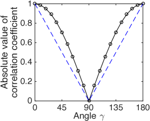
Figure 1: The curve of the absolute value of Pearson’s correlation coefficient against the angle $\gamma$ between two zero-mean variables.

It shows the curve of $|\rho_{{\bf{ab}}}|$ against the angle $\gamma$ within the intervals $[0^{\circ},180^{\circ}]$ in Figure 1, from which we can see that the absolute value of Pearson’s correlation coefficient is a good bivariate correlation measurement for two reasons. Firstly, the curve of $|\rho_{{\bf{ab}}}|$ against the angle $\gamma$ is always kept the opposite trend of change of the angle $\gamma^{*}$. Secondly, the strength of correlation measured by the absolute value of Pearson’s correlation coefficient (the black curve in Figure 1) is close to the strength of correlation measured by the angle $\gamma^{*}$ (the blue dotted segments in Figure 1).

Pearson’s correlation coefficient can only describe the correlation relationship between two variables. Lots of applications, such as data dimensionality reduction, subset selection, and sparse regression, need a correlation measurement to measure the strength of correlation among multiple variables. These applications usually select several variables from a number of variables to make the selected variables have the minimum correlation while maintaining enough information.

The development of information technology and big data analytics further increases the importance of multivariate correlation analysis. Unfortunately, there is no compact formulation to define and measure correlation for multiple variables. People have to estimate the strength of multivariate correlation by the indirect methods such as the partial correlation and the coefficient of determination. However, for most systems, such as physical, sociological, and economic systems, it is more important to discover associations among more than two variables.

In this paper, an unsigned correlation coefficient (UCC) and an unsigned incorrelation coefficient (UIC) are proposed. The proposed UCC and UIC can be used to measure the strength of multivariate correlation and linear irrelevance. Many properties of them are introduced in the paper. For example, both the proposed UCC and UIC belong to an interval [0,1]; The sum of the squared UCC and the squared UIC of a group of variables is always 1; The value of UCC for multiple non-zero-variance variables achieves the maximum value 1 if and only if these variables are linear dependent, and achieves the minimum value 0 if and only if these variables are perpendicular to each other; The value of UCC for a group of variables is not less than the value of UCC for part of them; If the number of variables is the same as their dimension, their UIC then equals to the absolute value of the determinant of the square matrix whose row or column vectors are the standardized vectors of these variables.

We also show that the value of UIC for multivate variables is the volume of the parallelotope formed by the standardized vectors of them. Then we visually display that the strength of correlation of three variables measured by the unsigned tri-variate correlation coefficient is very close to the strength of correlation measured by a spatial angle $\eta$.

All the properties and the figures of UCC and UIC show that the proposed UCC and UIC are the general measures of correlation for multiple variables.

2.  INNER PRODUCT-DETERMINANT EQUATION

If two non-zero-variance variables ${\bf{a}}$ and ${\bf{b}}$ are linear dependent, we have $\rho^{2}_{{\bf{ab}}}=1$. Garnett had proved that if three non-zero-variance variables ${\bf{a}}$, ${\bf{b}}$, and ${\bf{c}}$ are linear dependent, then $\rho_{{\bf{ab}}}^{2}+\rho_{{\bf{bc}}}^{2}+\rho_{{\bf{ac}}}^{2}-2\rho_{{\bf{ab}}}\rho_{{\bf{bc}}}\rho_{{\bf{ac}}}=1$ [3].

For two variables ${\bf{a}}$ and ${\bf{b}}$, we use $|\rho_{{\bf{ab}}}|$ to measure the strength of correlation between them. According to the above discussion, we analyze the relation of the strength of correlation among ${\bf{a}}$, ${\bf{b}}$, and ${\bf{c}}$ with the value of $r_{{\bf{abc}}}=\sqrt{\rho_{{\bf{ab}}}^{2}+\rho_{{\bf{bc}}}^{2}+\rho_{{\bf{ac}}}^{2}-2\rho_{{\bf{ab}}}\rho_{{\bf{bc}}}\rho_{{\bf{ac}}}}$.

According to Garnett’s conclusion, $r_{{\bf{abc}}}=1$ if and only if variables ${\bf{a}}$, ${\bf{b}}$, and ${\bf{c}}$ on the same plane. Moreover, it is obviously that $r_{{\bf{abc}}}=0$ if and only if variables ${\bf{a}}$, ${\bf{b}}$, and ${\bf{c}}$ are perpendicular to each other. The two important properties of $r_{{\bf{abc}}}$ show that $r_{{\bf{abc}}}$ may be a proper measurement to measure the strength of correlation among three variables.

We denote by ${\bf{a}}^{\prime}$ the standardized vector of the non-zero-variance vector ${\bf{a}}$:

$${\bf{a}}^{\prime}=\frac{{\bf{a}}-{\mu_{\bf{a}}}{\bf{1}}}{\left\|{\bf{a}}-{\mu_{\bf{a}}}{\bf{1}}\right\|}.$$

If ${\bf{a}}{\rm{{}^{\prime}}}$ and ${\bf{b}}{\rm{{}^{\prime}}}$ are the standardized vectors of ${\bf{a}}$ and ${\bf{b}}$, respectively, Pearson’s correlation coefficient between ${\bf{a}}$ and ${\bf{b}}$ is then the inner product between ${\bf{a}}{\rm{{}^{\prime}}}$ and ${\bf{b}}{\rm{{}^{\prime}}}$, and $r_{{\bf{abc}}}$ can also be expressed by the inner product of ${\bf{a}}{\rm{{}^{\prime}}}$ and ${\bf{b}}{\rm{{}^{\prime}}}$, the inner product of ${\bf{a}}{\rm{{}^{\prime}}}$ and ${\bf{c}}{\rm{{}^{\prime}}}$, and the inner product of ${\bf{b}}{\rm{{}^{\prime}}}$ and ${\bf{c}}{\rm{{}^{\prime}}}$.

Here we focus on an identical relation between inner product and a determinant group, which we call the inner product-determinant equation (IPD equation).

For $n$-dimensional variables ${\bf{a}}_{1}$, ${\bf{a}}_{2}$, $\cdots$, and ${\bf{a}}_{m}$, ${\bf{a}}_{i}=(a_{i1},a_{i2},\cdots$, $a_{in})^{T}$, $i=1,2,\cdots$, $m$, $m\leq n$, we denote

$$[{\bf{a}}(m)|j_{1},j_{2},\cdots,j_{m}]=\left[{\begin{array}[]{*{20}c}{a_{1j_{1}}}&{a_{1j_{2}}}&\cdots&{a_{1j_{m}}}\\ {a_{2j_{1}}}&{a_{2j_{2}}}&\cdots&{a_{2j_{m}}}\\ \vdots&\vdots&\ddots&\vdots\\ {a_{mj_{1}}}&{a_{mj_{2}}}&\cdots&{a_{mj_{m}}}\\ \end{array}}\right],$$

where $1\leq j_{1}<j_{2}<\cdots<j_{m}\leq n$.

According to Cauchy-Binet formula [4], we have the following lemma:

Lemma 1  For $n$-dimensional variables ${\bf{a}}_{1}$, ${\bf{a}}_{2}$, $\cdots$, and ${\bf{a}}_{m}$, ${\bf{a}}_{i}=(a_{i1},a_{i2},\cdots,a_{in})^{T}$, $i\in\{1,2,\cdots,m\}$, $m\leq n$, if ${\bf{M}}$ is the inner product matrix of these variables,

$${\bf{M}}=\left[{\begin{array}[]{*{20}c}{<\!{\bf{a}}_{1},{\bf{a}}_{1}\!>}&{<\!{\bf{a}}_{1},{\bf{a}}_{2}\!>}&\cdots&{<\!{\bf{a}}_{1},{\bf{a}}_{m}\!>}\\ {<\!{\bf{a}}_{2},{\bf{a}}_{1}\!>}&{<\!{\bf{a}}_{2},{\bf{a}}_{2}\!>}&\cdots&{<\!{\bf{a}}_{2},{\bf{a}}_{m}\!>}\\ \vdots&\vdots&\ddots&\vdots\\ {<\!{\bf{a}}_{m},{\bf{a}}_{1}\!>}&{<\!{\bf{a}}_{m},{\bf{a}}_{2}\!>}&\cdots&{<\!{\bf{a}}_{m},{\bf{a}}_{m}\!>}\\ \end{array}}\right],$$

then we have

$$\det({\bf{M}})=\sum\limits_{j_{1}<j_{2}<\cdots<j_{m}}{(\det[{\bf{a}}(m)|j_{1},j_{2},\cdots,j_{m}])^{2}},$$ (2)

where $j_{1},j_{2},\cdots,j_{m}\in\{1,2,\cdots,n\}$.

Proof: According to Cauchy-Binet formula, for the matrixes ${\bf{A}}=[{\bf{a}}_{1},{\bf{a}}_{2},\cdots,{\bf{a}}_{m}]$ and ${\bf{A}}^{T}$, we have

$$\det({\bf{A}}^{T}{\bf{A}})=\sum\limits_{j_{1}<j_{2}<\cdots<j_{m}}{(\det[{\bf{a}}(m)|j_{1}<j_{2}<\cdots<j_{m}])^{2}}.$$

Because ${\bf{A}}^{T}{\bf{A}}={\bf{M}}$, this lemma is true. $\blacksquare$

We denote by $\Gamma$ the circular inner product

$$\begin{array}[]{l}\Gamma\!\!<\!{\bf{a}}_{k_{1}},{\bf{a}}_{k_{2}},\cdots,{\bf{a}}_{k_{p}}\!>=<\!{\bf{a}}_{k_{1}},{\bf{a}}_{k_{2}}\!><\!{\bf{a}}_{k_{2}},{\bf{a}}_{k_{3}}\!>\cdots<\!{\bf{a}}_{k_{p-1}},{\bf{a}}_{k_{p}}\!><\!{\bf{a}}_{k_{p}},{\bf{a}}_{k_{1}}\!>.\end{array}$$ (3)

For a group of variables, all the permutations of them which can generate the same inner product or circular inner product are regarded as the same inner-product-permutation, then the inner product-determinant equation can be rewritten as following:

Inner product-Determinant Equation  For $n$-dimensional variables ${\bf{a}}_{1}$, ${\bf{a}}_{2}$, $\cdots$, and ${\bf{a}}_{m}$, $m\leq n$, the inner-product-determinant equation is

$$\begin{array}[]{l}\sum\limits_{\pi}{2^{\left|{\pi_{3}}\right|}(-1)^{m-\left|{\pi}\right|}}{\prod\limits_{\pi_{1}}\left\|{{\bf{a}}_{s}}\right\|^{2}\prod\limits_{\pi_{2}}{<\!{\bf{a}}_{i},{\bf{a}}_{j}\!>^{2}}}\prod\limits_{\pi_{3}}{\Gamma\!\!<\!{\bf{a}}_{k_{1}},{\bf{a}}_{k_{2}},\cdots,{\bf{a}}_{k_{p}}\!>}\\ =\sum\limits_{j_{1}<j_{2}<\cdots<j_{m}}{(\det[{\bf{a}}(m)|j_{1},j_{2},\cdots,j_{m}])^{2}},\end{array}$$ (4)

where $\pi$ runs through the list of all partitions of $\{{\bf{a}}_{1},{\bf{a}}_{2},\cdots$, ${\bf{a}}_{m}\}$ with only consider the inner-product-permutation, and the subsets in each partition $\pi$ are divided into three classes: If one subset only contains one variable, then this subset belongs to the first class $\pi_{1}$, and the self-inner product of the variable appears in the formula of the partition; If one subset contains two different variables, then this subset belongs to the second class $\pi_{2}$, and the square of mutual inner product between the two variables appears in the formula of the partition; The others belong to the third class $\pi_{3}$, and the circular inner product for each subset in $\pi_{3}$ appears in the formula of the partition; The number of subsets in a partition $\pi$ and $\pi_{3}$ are $\left|{\pi}\right|$ and $\left|{\pi_{3}}\right|$, respectively.

Proof: In fact, each partition $\pi$ in the inner product-determinant equation is corresponding to one item in the expansion of the determinant of the inner product matrix. By considering the inversion number and the symmetry of inner product matrix, the above equation can be easily obtained. $\blacksquare$

If the number of subsets in each $\pi_{1}$ and $\pi_{2}$ are $\left|{\pi_{1}}\right|$ and $\left|{\pi_{2}}\right|$, respectively, then $\left|{\pi_{1}}\right|+\left|{\pi_{2}}\right|+\left|{\pi_{3}}\right|=\left|{\pi}\right|$. Moreover, the subsets in $\pi_{3}$ are not the standard sets because the inner-product-permutation is involved.

The inner product-determinant equation has a set-partition-based form, which is similar to the joint cumulant equation [5, 6].

For three $n$-dimensional variables ${\bf{a}}$, ${\bf{b}}$, and ${\bf{c}}$, $n\geq 3$, there are 6 cases of inner products in total, and they are $<\!{\bf{a}},{\bf{a}}\!>$, $<\!{\bf{b}},{\bf{b}}\!>$, $<\!{\bf{c}},{\bf{c}}\!>$, $<\!{\bf{a}},{\bf{b}}\!>$, $<\!{\bf{a}},{\bf{c}}\!>$, and $<\!{\bf{b}},{\bf{c}}\!>$. From Lemma 1, the IPD equation for three variables can be obtained as following:

Corollary 1  For three $n$-dimensional variables ${\bf{a}}$, ${\bf{b}}$, and ${\bf{c}}$, $n\geq 3$, the inner product-determinant equation is as following:

$$\begin{array}[]{l}\left\|{\bf{a}}\right\|^{2}\left\|{\bf{b}}\right\|^{2}\left\|{\bf{c}}\right\|^{2}-\left\|{\bf{a}}\right\|^{2}\!<\!{\bf{b}},{\bf{c}}\!>^{2}\!-\left\|{\bf{b}}\right\|^{2}\!<\!{\bf{a}},{\bf{c}}\!>^{2}\!-\left\|{\bf{c}}\right\|^{2}\!<\!{\bf{a}},{\bf{b}}\!>^{2}\!\\ +2<\!{\bf{a}},{\bf{b}}\!><\!{\bf{b}},{\bf{c}}\!><\!{\bf{a}},{\bf{c}}\!>\ =\sum\limits_{i<j<k}{<\!\det[{\bf{a}},{\bf{b}},{\bf{c}}|i,j,k]\!>^{2}},\end{array}$$ (5)

where $i,j,k\in\{1,2,\cdots,n\}$.

Similarly, IPD equation for two variables is listed below.

Corollary 2  For two $n$-dimensional variables ${\bf{a}}$ and ${\bf{b}}$, $n\geq 2$, the inner product-determinant equation is

$$\left\|{\bf{a}}\right\|^{2}\left\|{\bf{b}}\right\|^{2}-<\!{\bf{a}},{\bf{b}}\!>^{2}=\sum\limits_{i<j}{(\det[{\bf{a}},{\bf{b}}|i,j])^{2}},$$ (6)

where $i,j\in\{1,2,\cdots,n\}$.

3.  CORRELATION MEASURES FOR MULTIPLE VARIABLES

According to Corollary 1, if ${\bf{a}}{\rm{{}^{\prime}}}$, ${\bf{b}}{\rm{{}^{\prime}}}$, and ${\bf{c}}{\rm{{}^{\prime}}}$ are the standardized vectors of ${\bf{a}}$, ${\bf{b}}$, and ${\bf{c}}$, respectively, we have

$$r_{{\bf{abc}}}^{2}=1-\sum\limits_{i<j<k}{(\det[{\bf{a}}^{\prime},{\bf{b}}^{\prime},{\bf{c}}^{\prime}|i,j,k])^{2}}.$$ (7)

Similarly, the square of Pearson’s correlation coefficient between ${\bf{a}}$ and ${\bf{b}}$ can be obtained from Corollary 2:

$$\rho_{{\bf{ab}}}^{2}=1-\sum\limits_{i<j}{(\det[{\bf{a}}^{\prime},{\bf{b}}^{\prime}|i,j])^{2}}.$$ (8)

Inspired by the above formulas of $r_{{\bf{abc}}}^{2}$ and $\rho_{{\bf{ab}}}^{2}$, we define the multivariate correlation measurement as following:

Definition 1  For $n$-dimensional non-zero-variance variables ${\bf{a}}_{1}$, ${\bf{a}}_{2}$, $\cdots$, ${\bf{a}}_{m}$, $2\leq m\leq n$, if ${\bf{a}}^{\prime}_{i}=(a^{\prime}_{i1},a^{\prime}_{i2},\cdots,a^{\prime}_{in})^{T}$ is the standardized vector of ${\bf{a}}_{i}=(a_{i1},a_{i2},\cdots,a_{in})^{T}$, $i\in\{1,2,\cdots,m\}$, then the unsigned correlation coefficient $r_{{\bf{a}}_{1}{\bf{a}}_{2}\cdots{\bf{a}}_{m}}$ among ${\bf{a}}_{1}$, ${\bf{a}}_{2}$, $\cdots$, and ${\bf{a}}_{m}$ is defined as

$$\begin{array}[]{l}r_{{\bf{a}}_{1}{\bf{a}}_{2}\cdots{\bf{a}}_{m}}^{2}=1-\sum\limits_{j_{1}<j_{2}<\cdots<j_{m}}{(\det[{\bf{a}}^{\prime}(m)|j_{1},j_{2},\cdots,j_{m}])^{2}}\\ \end{array},$$ (9)

where

$$[{\bf{a}}^{\prime}(m)|j_{1},j_{2},\cdots,j_{m}]=\left[{\begin{array}[]{*{20}c}{a^{\prime}_{1j_{1}}}&{a^{\prime}_{1j_{2}}}&\cdots&{a^{\prime}_{1j_{m}}}\\ {a^{\prime}_{2j_{1}}}&{a^{\prime}_{2j_{2}}}&\cdots&{a^{\prime}_{2j_{m}}}\\ \vdots&\vdots&\ddots&\vdots\\ {a^{\prime}_{mj_{1}}}&{a^{\prime}_{mj_{2}}}&\cdots&{a^{\prime}_{mj_{m}}}\\ \end{array}}\right],$$

$j_{1},j_{2},\cdots,j_{m}\in\{1,2,\cdots,n\}$ and $1\leq j_{1}<j_{2}<\cdots<j_{m}\leq n$.

The sign of mutual direction for two variables can be judged by whether the angle between the zero-mean variables of them is larger than $90^{\circ}$. However, there is no the mutual direction for multiple variables. Therefore, the correlation measurement for multiple variables in this paper is defined as an unsigned value, the rationality of which is also discussed in Section 3 in this paper.

According to Definition 1, for two non-zero-variance variables ${\bf{a}}$ and ${\bf{b}}$, $r_{{\bf{ab}}}=|\rho_{{\bf{ab}}}|$. Then we can see that the sum of the squares of the determinant group is a coupling part of the proposed UCC. We define the coupling part as the square of the unsigned incorrelation coefficient (UIC), which can be used to measure linear irrelevance among variables:

Definition 2  For $n$-dimensional non-zero-variance variables ${\bf{a}}_{1}$, ${\bf{a}}_{2}$, $\cdots$, ${\bf{a}}_{m}$, $2\leq m\leq n$, if ${\bf{a}}^{\prime}_{i}$ is the standardized vector of ${\bf{a}}_{i}$, $i\in\{1,2,\cdots,m\}$, the unsigned incorrelation coefficient (UIC) $\omega_{{\bf{a}}_{1}{\bf{a}}_{2}\cdots{\bf{a}}_{m}}$ among ${\bf{a}}_{1}$, ${\bf{a}}_{2}$, $\cdots$, and ${\bf{a}}_{m}$ is defined as

$$\begin{array}[]{l}\omega_{{\bf{a}}_{1}{\bf{a}}_{2}\cdots{\bf{a}}_{m}}^{2}=\sum\limits_{j_{1}<j_{2}<\cdots<j_{m}}{(\det[{\bf{a}}^{\prime}(m)|j_{1},j_{2},\cdots,j_{m}])^{2}},\end{array}$$ (10)

where $j_{1},j_{2},\cdots,j_{m}\in\{1,2,\cdots,n\}$ and $1\leq j_{1}<j_{2}<\cdots<j_{m}\leq n$.

A lemma exists for UIC as following:

Lemma 2  For $n$-dimensional variables ${\bf{a}}_{1}$, ${\bf{a}}_{2}$, $\cdots$, ${\bf{a}}_{m}$, ${\bf{a}}_{m+1}$, $2\leq{m+1}\leq n$, if ${\bf{a}}^{\prime}_{i}$ is the standardized vector of ${\bf{a}}_{i}$, $i=1,2,\cdots,m,m+1$, we have

$$\begin{array}[]{l}\omega_{{\bf{a}}_{1}{\bf{a}}_{2}\cdots{\bf{a}}_{m}}^{2}-\omega_{{\bf{a}}_{1}{\bf{a}}_{2}\cdots{\bf{a}}_{m}{\bf{a}}_{m+1}}^{2}\\ =\sum\limits_{J_{m-1}}{(\sum\limits_{p\notin J_{m-1}}{(-1)^{g(p:J_{m-1})}a^{\prime}_{m+1,p}\det[{\bf{a}}^{\prime}(m)|p,J_{m-1}]})^{2}}\end{array},$$ (11)

where $J_{m-1}=\{j_{1},j_{2},\cdots,j_{m-1}\}$, $j_{1}$$<$$j_{2}$$<$$\cdots$$<$$j_{m-1}$, $j_{1}$, $j_{2}$, $\cdots$, $j_{m-1}$ $\in\{1,2,\cdots,n\}$, and $g(p:S)$ is the number of elements which are larger than $p$ in the set $S$.

Proof: Let $J_{m}=\{j^{\dagger}_{1},j^{\dagger}_{2},\cdots,j^{\dagger}_{m}\}$, $j^{\dagger}_{1}$$<$$j^{\dagger}_{2}$$<$$\cdots$$<$$j^{\dagger}_{m}$, $j^{\dagger}_{1}$, $j^{\dagger}_{2}$, $\cdots$, $j^{\dagger}_{m}$ $\in\{1$, $2,\cdots,n\}$, and $J_{m+1}=\{j^{\ddagger}_{1},j^{\ddagger}_{2},\cdots$, $j^{\ddagger}_{m},j^{\ddagger}_{m+1}\}$, $j^{\ddagger}_{1}$$<$$j^{\ddagger}_{2}$$<$$\cdots$$<$$j^{\ddagger}_{m}$$<$$j^{\ddagger}_{m+1}$, $j^{\ddagger}_{1}$, $j^{\ddagger}_{2}$, $\cdots$, $j^{\ddagger}_{m}$, $j^{\ddagger}_{m+1}$ $\in\{1$, $2,\cdots,n\}$.

$$\begin{array}[]{l}\omega_{{\bf{a}}_{1}{\bf{a}}_{2}\cdots{\bf{a}}_{m}{\bf{a}}_{m+1}}^{2}=\sum\limits_{J_{m+1}}{(\det[{\bf{a}}^{\prime}(m+1)|J_{m+1}])^{2}}\\ =\sum\limits_{J_{m+1}}{\{\sum\limits_{p=j_{1}}^{j_{m+1}}{({a^{\prime}}_{m+1,p}^{2}\det^{2}[{\bf{a}}^{\prime}(m)|J_{m+1}\backslash p])}}\\ +\sum\limits_{\scriptstyle l,p\in J_{m+1}\hfill\atop\scriptstyle\quad\,l\neq p\hfill}\begin{array}[]{l}[2(-1)^{g(l:J_{m+1})}(a^{\prime}_{m+1,l}\det[{\bf{a}}^{\prime}(m)|J_{m+1}\backslash l])\\ (-1)^{g(p:J_{m+1})}(a^{\prime}_{m+1,p}\det[{\bf{a}}^{\prime}(m)|J_{m+1}\backslash p])]\\ \end{array}\}.\\ \end{array}$$

The first part can be rewritten as

$$\begin{array}[]{l}\sum\limits_{J_{m+1}}{\sum\limits_{p=j_{1}}^{j_{m+1}}{({a^{\prime}}_{m+1,p}^{2}\det^{2}[{\bf{a}}^{\prime}(m)|J_{m+1}\backslash p])}}=\sum\limits_{p}{{a^{\prime}}_{m+1,p}^{2}}\sum\limits_{\scriptstyle\ \,J_{m}\hfill\atop\scriptstyle p\notin J_{m}\hfill}{\det^{2}[{\bf{a}}^{\prime}(m)|J_{m}]}\\ =\sum\limits_{p}{{a^{\prime}}_{m+1,p}^{2}}(\omega_{{\bf{a}}_{1}{\bf{a}}_{2}\cdots{\bf{a}}_{m}}^{2}-\sum\limits_{\scriptstyle\ \,J_{m}\hfill\atop\scriptstyle p\in J_{m}\hfill}{\det^{2}[{\bf{a}}^{\prime}(m)|J_{m}])}\\ =\left\|{{\bf{a}}^{\prime}_{m+1}}\right\|^{2}\omega_{{\bf{a}}_{1}{\bf{a}}_{2}\cdots{\bf{a}}_{m}}^{2}-\sum\limits_{p}{{a^{\prime}}_{m+1,p}^{2}}\sum\limits_{\scriptstyle\ \,J_{m}\hfill\atop\scriptstyle p\in J_{m}\hfill}{\det^{2}[{\bf{a}}^{\prime}(m)|J_{m}]}\\ =\omega_{{\bf{a}}_{1}{\bf{a}}_{2}\cdots{\bf{a}}_{m}}^{2}-\sum\limits_{p}{{a^{\prime}}_{m+1,p}^{2}}\sum\limits_{\scriptstyle\ J_{m-1}\hfill\atop\scriptstyle p\notin J_{m-1}\hfill}{\det^{2}[{\bf{a}}^{\prime}(m)|p,J_{m-1}]},\\ \end{array}$$

and the second part can be rewritten as

$$\begin{array}[]{l}\sum\limits_{J_{m+1}}{\sum\limits_{\scriptstyle l,p\in J_{m+1}\hfill\atop\scriptstyle\quad\ l\neq p\hfill}\begin{array}[]{l}\{2(-1)^{g(l:J_{m+1})+g(p:J_{m+1})}a^{\prime}_{m+1,l}a^{\prime}_{m+1,p}\\ \det[{\bf{a}}^{\prime}(m)|J_{m+1}\backslash l]\det[{\bf{a}}^{\prime}(m)|J_{m+1}\backslash p]\}\\ \end{array}}\\ =2\sum\limits_{l\neq p}{a^{\prime}_{m+1,l}a^{\prime}_{m+1,p}\sum\limits_{\scriptstyle\quad J_{m+1}\hfill\atop\scriptstyle\ l,p\in J_{m+1}\hfill}\begin{array}[]{l}\{(-1)^{g(l:J_{m+1})+g(p:J_{m+1})}\\ \det[{\bf{a}}^{\prime}(m)|J_{m+1}\backslash l]\det[{\bf{a}}^{\prime}(m)|J_{m+1}\backslash p]\}\\ \end{array}}\\ =2\sum\limits_{l\neq p}{a^{\prime}_{m+1,l}a^{\prime}_{m+1,p}\sum\limits_{\scriptstyle\quad J_{m-1}\hfill\atop\scriptstyle l,p\notin J_{m-1}\hfill}\begin{array}[]{l}\{(-1)^{g(l:J_{m-1})+g(p:J_{m-1})+1}\\ \det[{\bf{a}}^{\prime}(m)|p,J_{m-1}]\det[{\bf{a}}^{\prime}(m)|l,J_{m-1}]\}\\ \end{array}}\\ =-2\sum\limits_{J_{m-1}}{\sum\limits_{{\scriptstyle\quad\,l\neq p\hfill\atop\scriptstyle l,p\notin J_{m-1}\hfill}}\begin{array}[]{l}\{(-1)^{g(p:J_{m-1})}a^{\prime}_{m+1,p}\det[{\bf{a}}^{\prime}(m)|p,J_{m-1}]\\ (-1)^{g(l:J_{m-1})}a^{\prime}_{m+1,l}\det[{\bf{a}}^{\prime}(m)|l,J_{m-1}]\}\\ \end{array}}.\\ \end{array}$$

Hence, we have

$$\omega_{{\bf{a}}_{1}{\bf{a}}_{2}\cdots{\bf{a}}_{m}{\bf{a}}_{m+1}}^{2}=\omega_{{\bf{a}}_{1}{\bf{a}}_{2}\cdots{\bf{a}}_{m}{\bf{a}}_{m}}^{2}-\phi({\bf{a}}^{\prime}(m+1)),$$

and $\phi({\bf{a}}^{\prime}(m+1))$ can be expressed as

$$\begin{array}[]{l}\phi({\bf{a}}^{\prime}(m+1))=\sum\limits_{J_{m-1}}{\sum\limits_{p\notin J_{m-1}}\begin{array}[]{l}{a^{\prime}}_{m+1,p}^{2}\det^{2}[{\bf{a}}^{\prime}(m)|p,J_{m-1}]\\ \end{array}}\\ +2\sum\limits_{J_{m-1}}{\sum\limits_{{\scriptstyle\quad\,l\neq p\hfill\atop\scriptstyle l,p\notin J_{m-1}\hfill}}\begin{array}[]{l}\{(-1)^{g(p:J_{m-1})}a^{\prime}_{m+1,p}\det[{\bf{a}}^{\prime}(m)|p,J_{m-1}]\\ \cdot(-1)^{g(l:J_{m-1})}a^{\prime}_{m+1,l}\det[{\bf{a}}^{\prime}(m)|l,J_{m-1}]\}\\ \end{array}}\\ =\sum\limits_{J_{m-1}}{(\sum\limits_{p\notin J_{m-1}}\begin{array}[]{l}(-1)^{g(p:J_{m-1})}a^{\prime}_{m+1,p}\det[{\bf{a}}^{\prime}(m)|p,J_{m-1}])^{2}.\\ \end{array}}\\ \end{array}$$

$\blacksquare$

The proposed unsigned correlation coefficient and unsigned incorrelation coefficient have some important properties, several of which are discussed below.

Property 3.1  $r_{{\bf{a}}_{1}{\bf{a}}_{2}\cdots{\bf{a}}_{m}}$ and $\omega_{{\bf{a}}_{1}{\bf{a}}_{2}\cdots{\bf{a}}_{m}}$ are both the symmetric functions of ${\bf{a}}_{1}$, ${\bf{a}}_{2}$, $\cdots$, ${\bf{a}}_{m}$.

Property 3.2  If $r_{{\bf{a}}_{1}{\bf{a}}_{2}\cdots{\bf{a}}_{m}}$ and $\omega_{{\bf{a}}_{1}{\bf{a}}_{2}\cdots{\bf{a}}_{m}}$ are UCC and UIC for non-zero-variance variables ${\bf{a}}_{1}$, ${\bf{a}}_{2}$, $\cdots$, ${\bf{a}}_{m}$, respectively, and $r_{{\bf{a}}_{1}{\bf{a}}_{2}\cdots{\bf{a}}_{m-1}}$ and $\omega_{{\bf{a}}_{1}{\bf{a}}_{2}\cdots{\bf{a}}_{m-1}}$ are UCC and UIC for ${\bf{a}}_{1}$, ${\bf{a}}_{2}$, $\cdots$, ${\bf{a}}_{m-1}$, respectively, then

$$\begin{array}[]{l}r_{{\bf{a}}_{1}{\bf{a}}_{2}\cdots{\bf{a}}_{m}}^{2}\geq r_{{\bf{a}}_{1}{\bf{a}}_{2}\cdots{\bf{a}}_{m-1}}^{2}\\ \omega_{{\bf{a}}_{1}{\bf{a}}_{2}\cdots{\bf{a}}_{m}}^{2}\leq\omega_{{\bf{a}}_{1}{\bf{a}}_{2}\cdots{\bf{a}}_{m-1}}^{2}\\ \end{array}$$

Property 3.2 can be directly obtained from Lemma 2. It shows that the value of UCC for some variables is not less than the value of UCC for part of the variables.

Property 3.3

$$\begin{array}[]{l}0\leq r_{{\bf{a}}_{1}{\bf{a}}_{2}\cdots{\bf{a}}_{m}}^{2}\leq 1\\ 0\leq\omega_{{\bf{a}}_{1}{\bf{a}}_{2}\cdots{\bf{a}}_{m}}^{2}\leq 1\\ \end{array}$$

Proof: According to Definition 2 we have $\omega_{{\bf{a}}_{1}{\bf{a}}_{2}\cdots{\bf{a}}_{m}}^{2}\geq 0$. From Property 3.2, $\omega_{{\bf{a}}_{1}{\bf{a}}_{2}\cdots{\bf{a}}_{m}}^{2}$ $\leq$ $\cdots\leq\omega_{{\bf{a}}_{i}{\bf{a}}_{j}}^{2}=1-\rho_{{\bf{a}}_{i}{\bf{a}}_{j}}^{2}\leq 1$, $i$$\neq$$j,\ i,j\in\{1,2,\cdots,m\}$. Because $r_{{\bf{a}}_{1}{\bf{a}}_{2}\cdots{\bf{a}}_{m}}^{2}+\omega_{{\bf{a}}_{1}{\bf{a}}_{2}\cdots{\bf{a}}_{m}}^{2}=1$, we have $0\leq r_{{\bf{a}}_{1}{\bf{a}}_{2}\cdots{\bf{a}}_{m}}^{2}\leq 1$. $\blacksquare$

Property 3.4  $r_{{\bf{a}}_{1}{\bf{a}}_{2}\cdots{\bf{a}}_{m}}^{2}=1$ if and only if variables ${\bf{a}}_{1},{\bf{a}}_{2},\cdots$, and ${\bf{a}}_{m}$ are linear dependent.

Proof:

Sufficiency: If ${\bf{a}}_{1},{\bf{a}}_{2},\cdots$, and ${\bf{a}}_{m}$ are linear dependent, $\det[{\bf{a}}^{\prime}(m)|j_{1},j_{2}$, $\cdots,j_{m}]=0$ for all cases of $j_{1}<j_{2}<\cdots<j_{m}$, $j_{1},j_{2},\cdots,j_{m}\in\{1,2,\cdots,n\}$.

Necessity: We denote by ${\mathop{\bf{a}}\limits^{\wedge}}_{j}={(a_{1j},a_{2j},\cdots,a_{mj})^{T}}$ the $j$th column vector of the matrix [${\bf{a}}(m)|1,2$, $\cdots$, $n$], $j=1,2,\cdots,n$. Presume that $j_{1},j_{2},\cdots,j_{m}$ exist to make rank$\{{\mathop{\bf{a}}\limits^{\wedge}}_{j_{1}},{\mathop{\bf{a}}\limits^{\wedge}}_{j_{2}},\cdots,{\mathop{\bf{a}}\limits^{\wedge}}_{j_{m}}\}=m$, then $\det[{\bf{a}}(m)|j_{1},j_{2},\cdots,j_{m}]\neq 0$ and $r_{{\bf{a}}_{1}{\bf{a}}_{2}\cdots{\bf{a}}_{m}}^{2}<1$. Hence, the presume is incorrect. We have rank$\{{\mathop{\bf{a}}\limits^{\wedge}}_{1},{\mathop{\bf{a}}\limits^{\wedge}}_{2},\cdots,{\mathop{\bf{a}}\limits^{\wedge}}_{n}\}$ $\leq m-1$ if $r_{{\bf{a}}_{1}{\bf{a}}_{2}\cdots{\bf{a}}_{m}}^{2}=1$. Because the row rank equals to the column rank of the same matrix, we have

$$\text{rank}\{{\bf{a}}_{1},{\bf{a_{2}}},\cdots,{\bf{a}}_{m}\}=\text{rank}\{{\mathop{\bf{a}}\limits^{\wedge}}_{1},{\mathop{\bf{a}}\limits^{\wedge}}_{2},\cdots,{\mathop{\bf{a}}\limits^{\wedge}}_{n}\}\leq m-1.$$

$\blacksquare$

For four variables ${\bf{a}}_{1},{\bf{a}}_{2},{\bf{a}}_{3}$, and ${\bf{a}}_{4}$, let $\rho_{{\bf{a}}_{i}{\bf{a}}_{j}}$ be Pearson’s correlation coefficient between the variables ${\bf{a}}_{i}$ and ${\bf{a}}_{j}$, $i,j\in\{1,2,3,4\}$. Then ${\bf{a}}_{1},{\bf{a}}_{2},{\bf{a}}_{3}$, and ${\bf{a}}_{4}$ are linear dependent if and only if

$$\begin{array}[]{l}\rho_{{\bf{a}}_{1}{\bf{a}}_{2}}^{2}+\rho_{{\bf{a}}_{1}{\bf{a}}_{3}}^{2}+\rho_{{\bf{a}}_{1}{\bf{a}}_{4}}^{2}+\rho_{{\bf{a}}_{2}{\bf{a}}_{3}}^{2}+\rho_{{\bf{a}}_{2}{\bf{a}}_{4}}^{2}+\rho_{{\bf{a}}_{3}{\bf{a}}_{4}}^{2}-(\rho_{{\bf{a}}_{1}{\bf{a}}_{2}}^{2}\rho_{{\bf{a}}_{3}{\bf{a}}_{4}}^{2}+\rho_{{\bf{a}}_{1}{\bf{a}}_{3}}^{2}\rho_{{\bf{a}}_{2}{\bf{a}}_{4}}^{2}+\rho_{{\bf{a}}_{1}{\bf{a}}_{4}}^{2}\rho_{{\bf{a}}_{2}{\bf{a}}_{3}}^{2})\\ -2(\rho_{{\bf{a}}_{1}{\bf{a}}_{3}}\rho_{{\bf{a}}_{1}{\bf{a}}_{4}}\rho_{{\bf{a}}_{3}{\bf{a}}_{4}}+\rho_{{\bf{a}}_{1}{\bf{a}}_{2}}\rho_{{\bf{a}}_{1}{\bf{a}}_{4}}\rho_{{\bf{a}}_{2}{\bf{a}}_{4}}+\rho_{{\bf{a}}_{1}{\bf{a}}_{2}}\rho_{{\bf{a}}_{1}{\bf{a}}_{3}}\rho_{{\bf{a}}_{2}{\bf{a}}_{3}}+\rho_{{\bf{a}}_{2}{\bf{a}}_{3}}\rho_{{\bf{a}}_{2}{\bf{a}}_{4}}\rho_{{\bf{a}}_{3}{\bf{a}}_{4}})\\ +2(\rho_{{\bf{a}}_{1}{\bf{a}}_{3}}\rho_{{\bf{a}}_{1}{\bf{a}}_{4}}\rho_{{\bf{a}}_{2}{\bf{a}}_{3}}\rho_{{\bf{a}}_{2}{\bf{a}}_{4}}+\rho_{{\bf{a}}_{1}{\bf{a}}_{2}}\rho_{{\bf{a}}_{1}{\bf{a}}_{4}}\rho_{{\bf{a}}_{2}{\bf{a}}_{3}}\rho_{{\bf{a}}_{3}{\bf{a}}_{4}}+\rho_{{\bf{a}}_{1}{\bf{a}}_{2}}\rho_{{\bf{a}}_{1}{\bf{a}}_{3}}\rho_{{\bf{a}}_{2}{\bf{a}}_{4}}\rho_{{\bf{a}}_{3}{\bf{a}}_{4}})=1\end{array},$$ (12)

which is also kept the same with Garnett’s results [3].

Property 3.5  $r_{{\bf{a}}_{1}{\bf{a}}_{2}\cdots{\bf{a}}_{m}}^{2}=0$ if and only if variables ${\bf{a}}_{1},{\bf{a}}_{2},\cdots$, and ${\bf{a}}_{m}$ are perpendicular to each other.

Proof:

$r_{{\bf{a}}_{1}{\bf{a}}_{2}\cdots{\bf{a}}_{m}}^{2}=0\Leftrightarrow\omega_{{\bf{a}}_{1}{\bf{a}}_{2}\cdots{\bf{a}}_{m}}^{2}=1$

According to Properties 3.2 and 3.3, we can obtain

$$1=\omega_{{\bf{a}}_{1}{\bf{a}}_{2}\cdots{\bf{a}}_{m}}^{2}\leq\cdots\leq\omega_{{\bf{a}}_{i}{\bf{a}}_{j}}^{2}\leq 1$$

Hence, for arbitrary $i,j\in{1,2,\cdots,m},i\neq j$, we have $\omega_{{\bf{a}}_{i}{\bf{a}}_{j}}^{2}=1$ and $r_{{\bf{a}}_{i}{\bf{a}}_{j}}^{2}=\rho_{{\bf{a}}_{i}{\bf{a}}_{j}}^{2}=0$.

$\blacksquare$

Property 3.6  If variables ${\bf{a}}_{1},{\bf{a}}_{2},\cdots,$ and ${\bf{a}}_{m-1}$ are not linear dependent, $r_{{\bf{a}}_{1}{\bf{a}}_{2}\cdots{\bf{a}}_{m}}^{2}$ then gets the biggest value 1 if and only if variable ${\bf{a}}_{m}$ lies on the hyperplane spanned by ${\bf{a}}_{1},{\bf{a}}_{2},\cdots,$ and ${\bf{a}}_{m-1}$, and $r_{{\bf{a}}_{1}{\bf{a}}_{2}\cdots{\bf{a}}_{m}}^{2}$ gets the smallest value $r_{{\bf{a}}_{1}{\bf{a}}_{2}\cdots{\bf{a}}_{m-1}}^{2}$ if and only if ${\bf{a}}_{m}$ is perpendicular to the hyperplane spanned by ${\bf{a}}_{1},{\bf{a}}_{2},\cdots,$ and ${\bf{a}}_{m-1}$.

Proof: The first half is true according to Property 3.4. Now we prove the second part.

According to Lemma 2, we have

$$\gamma_{{\bf{a}}_{1}{\bf{a}}_{2}\cdots{\bf{a}}_{m}}^{2}-\gamma_{{\bf{a}}_{1}{\bf{a}}_{2}\cdots{\bf{a}}_{m-1}}^{2}=\sum\limits_{J_{m-2}}{(\sum\limits_{p\notin J_{m-2}}\begin{array}[]{l}\!\!(-1)^{g(p:J_{m-2})}a^{\prime}_{m,p}\det[{\bf{a}}^{\prime}(m-1)|p,J_{m-2}])^{2}\\ \end{array}}.$$

Denote the determinant $\det(\mathop{i}\limits^{-};J_{m-2})$ as

$$\det(\mathop{i}\limits^{-};J_{m-2})=\det([{\bf{a}}^{\prime}_{1},{\bf{a}}^{\prime}_{2},\cdots,{\bf{a}}^{\prime}_{m-1}\backslash{\bf{a}}^{\prime}_{i}|J_{m-2}]).$$

Then we have

$$\begin{array}[]{l}\sum\limits_{p\notin J_{m-2}}{(-1)^{g(p:J_{m-2})}a^{\prime}_{m,p}}\det[{\bf{a}}^{\prime}(m-1)|p,J_{m-2}]\\ =\sum\limits_{p\notin J_{m-2}}{a^{\prime}_{m,p}}\sum\limits_{i}{(-1)^{i+1}a^{\prime}_{i,p}\det(\mathop{i}\limits^{-};J_{m-2})}\\ =\sum\limits_{i}{(-1)^{i+1}\det(\mathop{i}\limits^{-};J_{m-2})\sum\limits_{p\notin J_{m-2}}{a^{\prime}_{m,p}a^{\prime}_{i,p}}}\\ =\sum\limits_{i}{(-1)^{i+1}\det(\mathop{i}\limits^{-};J_{m-2})(\sum\limits_{p}{a^{\prime}_{m,p}a^{\prime}_{i,p}}-\sum\limits_{p\in J_{m-2}}{a^{\prime}_{m,p}a^{\prime}_{i,p}}})\\ =\sum\limits_{i}{(-1)^{i+1}\det(\mathop{i}\limits^{-};J_{m-2})({\bf{a}}^{\prime}_{i},{\bf{a}}^{\prime}_{m})}-\sum\limits_{i}{(-1)^{i+1}\det(\mathop{i}\limits^{-};J_{m-2})}\sum\limits_{p=j_{1}}^{j_{m-2}}{a^{\prime}_{m,p}a^{\prime}_{i,p}}\\ \end{array}$$

The first part of the above equation is a formula of the inner product. The second part can be simplified as

$$\begin{array}[]{l}\sum\limits_{i}{(-1)^{i+1}\det(\mathop{i}\limits^{-};j_{1},j_{2},\cdots,j_{m-2})}\sum\limits_{p=j_{1}}^{j_{m-2}}{a^{\prime}_{m,p}a^{\prime}_{i,p}}\\ =\det\!\!\left[{\begin{array}[]{*{20}c}{\!\!\sum\limits_{p=j_{1}}^{j_{m-2}}{a^{\prime}_{m,p}a^{\prime}_{i,p}}}&\!\!\!{a^{\prime}_{1,j_{1}}}&\!\!\!{a^{\prime}_{1,j_{2}}}&\!\!\!\cdots&\!\!\!{a^{\prime}_{1,j_{m-2}}}\\ {\!\!\sum\limits_{p=j_{1}}^{j_{m-2}}{a^{\prime}_{m,p}a^{\prime}_{i,p}}}&\!\!\!{a^{\prime}_{2,j_{1}}}&\!\!\!{a^{\prime}_{2,j_{2}}}&\!\!\!\cdots&\!\!\!{a^{\prime}_{2,j_{m-2}}}\\ \!\!\vdots&\!\!\!\vdots&\!\!\!\vdots&\!\!\!\ddots&\!\!\!\vdots\\ {\!\!\sum\limits_{p=j_{1}}^{j_{m-2}}{a^{\prime}_{m,p}a^{\prime}_{i,p}}}&\!\!\!{a^{\prime}_{m-1,j_{1}}}&\!\!\!{a^{\prime}_{m-1,j_{2}}}&\!\!\!\cdots&\!\!\!{a^{\prime}_{m-1,j_{m-2}}}\\ \end{array}}\!\!\!\!\right]\!=0\\ \end{array}$$

Hence,

$$\begin{array}[]{l}\sum\limits_{p\notin J_{m-2}}{(-1)^{g(p:J_{m-2})}a^{\prime}_{m,p}}\det[{\bf{a}}^{\prime}(m-1)|p,J_{m-2}]\\ =\sum\limits_{i=1}^{m-1}{(-1)^{i+1}\det(\mathop{i}\limits^{-};J_{m-2})({\bf{a}}^{\prime}_{i},{\bf{a}}^{\prime}_{m})}.\end{array}$$

Then $\gamma_{{\bf{a}}_{1}{\bf{a}}_{2}\cdots{\bf{a}}_{m}}^{2}$ gets the minimum value $r_{{\bf{a}}_{1}{\bf{a}}_{2}\cdots{\bf{a}}_{m-1}}^{2}$ if and only if

$$\sum\limits_{i=1}^{m-1}{(-1)^{i+1}\det(\mathop{i}\limits^{-};j_{1},j_{2},\cdots,j_{m-2})({\bf{a}}^{\prime}_{i},{\bf{a}}^{\prime}_{m})}=0$$ (13)

holds for all possible $\{j_{1},j_{2},\cdots,j_{m-2}\}$ and $i$.

Because variables ${\bf{a}}_{1},{\bf{a}}_{2},\cdots,{\bf{a}}_{m-1}$ are not linear dependent, $J_{m-1}=\{j_{1},j_{2},\cdots$, $j_{m-1}$} exists to make the rank of $[{\bf{a}}^{\prime}(m-1)|J_{m-1}]$ equal to $m-1$. Then $[{\bf{a}}^{\prime}(m-1)|J_{m-1}]$ is an invertible matrix and its adjoint matrix is also an invertible matrix. Each row of the adjoint matrix of $[{\bf{a}}^{\prime}(m-1)|J_{m-1}]$ is just the linear coefficients of one equation in the above equation. Finally, we obtain $({\bf{a}}^{\prime}_{i},{\bf{a}}^{\prime}_{m})=0,i=1,2,\cdots,m-1$. $\blacksquare$

According to Lemma 1 and Definition 2, if the number of variables is the same as their dimension, we have the following corollary, which gives a new explanation of determinant from the view of multivariate correlation.

Corollary 3  For $n$-dimensional non-zero-variance variables ${\bf{a}}_{1},{\bf{a}}_{2},\cdots$, and ${\bf{a}}_{n}$, if ${\bf{a}}^{\prime}_{i}$ is the standardized vector of ${\bf{a}}_{i}$, $i\in\{1,2,\cdots,n\}$, and ${\bf{A}}=[{\bf{a}}^{\prime}_{1},{\bf{a}}^{\prime}_{2},\cdots,{\bf{a}}^{\prime}_{n}]$, then we have

$$\omega_{{\bf{a}}_{1}{\bf{a}}_{2}\cdots{\bf{a}}_{m}}^{2}=(\det({\bf{A}}))^{2}.$$ (14)

This corollary gives a new explanation of determinant that if the row or column vectors of a matrix are all standardized, then the absolute value of the determinant of the matrix depicts the linear irrelevance of these standardized vectors.

Corollary 3 prompts us to consider the sign of the proposed UCC and UIC. If UIC is defined by the determinant of ${\bf{A}}$ when the number of variables is the same as their dimension, the value of UIC will have a positive or negative sign for a group of variables. However, because the sign of the determinant of ${\bf{A}}$ varies with the order of these variable appeared in the matrix ${\bf{A}}$, it is meaningless to take time to decide which sign is better. Moreover, the absolute value of correlation coefficient is more appropriate to measure the strength of correlation.

Lastly, if the variables in the inner product matrix ${\bf{M}}$ are all standardized vectors, the inner product matrix is then transformed into the correlation matrix. Correlation matrix is also a widely used tool in various fields. For $n$-dimensional non-zero-variance variables ${\bf{a}}_{1}$, ${\bf{a}}_{2}$, $\cdots$, ${\bf{a}}_{m}$, $2\leq m\leq n$, if $\rho_{ij}$ is Pearson’s correlation coefficient between ${\bf{a}}_{i}$ and ${\bf{a}}_{j}$, $i,j\in\{1,2,\cdots,m\}$, the correlation matrix ${\bf{R}}$ of these variables is as following:

$${\bf{R}}=\left[{\begin{array}[]{*{20}c}{\rho_{11}}&{\rho_{12}}&\cdots&{\rho_{1m}}\\ {\rho_{21}}&{\rho_{22}}&\cdots&{\rho_{2m}}\\ \vdots&\vdots&\ddots&\vdots\\ {\rho_{m1}}&{\rho_{m2}}&\cdots&{\rho_{mm}}\\ \end{array}}\right],$$

in which the diagonal elements are all 1.

Then we have the following Multivariate correlation Theorem from Lemma 1, Definition 1 and Definition 2:

Multivariate Correlation Theorem  If $r_{{\bf{a}}_{1}{\bf{a}}_{2}\cdots{\bf{a}}_{m}}$ and $\omega_{{\bf{a}}_{1}{\bf{a}}_{2}\cdots{\bf{a}}_{m}}$ are the unsigned correlation coefficient and the unsigned incorrelation coefficient for $n$-dimensional non-zero-variance variables ${\bf{a}}_{1}$, ${\bf{a}}_{2}$, $\cdots$, and ${\bf{a}}_{m}$, respectively, then

$$\begin{array}[]{l}\omega_{{\bf{a}}_{1}{\bf{a}}_{2}\cdots{\bf{a}}_{m}}^{2}=\det({\bf{R}})\\ r_{{\bf{a}}_{1}{\bf{a}}_{2}\cdots{\bf{a}}_{m}}^{2}=1-\det({\bf{R}})\end{array}.$$ (15)

Then according to the inner product-determinant equation, we have the UIC equation as following:

UIC Equation  For $n$-dimensional non-zero-variance variables ${\bf{a}}_{1}$, ${\bf{a}}_{2}$, $\cdots$, and ${\bf{a}}_{m}$, $m\leq n$,

$$\omega_{{\bf{a}}_{1}{\bf{a}}_{2}\cdots{\bf{a}}_{m}}^{2}=\sum\limits_{\pi}{2^{\left|{\pi_{3}}\right|}(-1)^{m-\left|{\pi}\right|}}{\prod\limits_{\pi_{2}}\rho^{2}_{{\bf{a}}_{i}{\bf{a}}_{j}}}\prod\limits_{\pi_{3}}{\Re\!\!<\!{\bf{a}}_{k_{1}},{\bf{a}}_{k_{2}},\cdots,{\bf{a}}_{k_{p}}\!>}$$ (16)

where $\Re\!\!<\!{\bf{a}}_{k_{1}},{\bf{a}}_{k_{2}},\cdots,{\bf{a}}_{k_{p}}\!>=\rho_{{\bf{a}}_{k_{1}}{\bf{a}}_{k_{2}}}\rho_{{\bf{a}}_{k_{2}}{\bf{a}}_{k_{3}}}\cdots\rho_{{\bf{a}}_{k_{p-1}}{\bf{a}}_{k_{p}}}\rho_{{\bf{a}}_{k_{p}}{\bf{a}}_{k_{1}}}$ is the circular correlation coefficient, and $\pi$, $\pi_{1}$, $\pi_{2}$, $\pi_{3}$, and $\left|{\pi_{3}}\right|$ are kept the same meanings as that in the inner product-determinant equation in which the inner products are replaced by correlation coefficients.

4.  VISUALIZATION ANALYSIS

Here we take the unsigned tri-variate correlation coefficient as an example to visually display the proposed UCC and discuss its effectiveness.

4.1  Visualization of the Proposed UCC

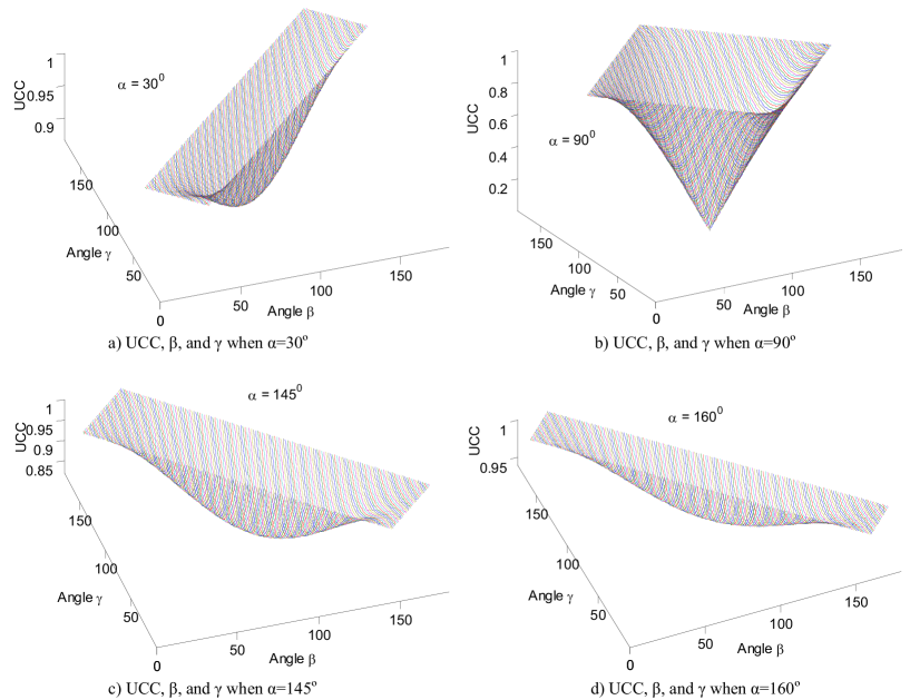
Figure 2: Some surfaces of the unsigned correlation coefficient against the angles $\beta$ and $\gamma$ with the other angle $\alpha$ fixed as $30^{0}$, $90^{0}$, $145^{0}$, and $160^{0}$, respectively.

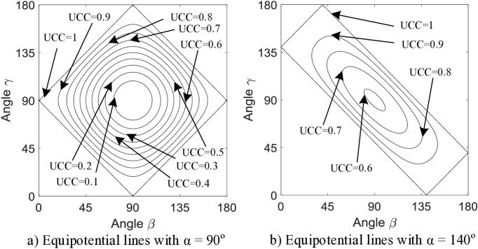
Figure 3: Some equipotential lines with different unsigned correlation coefficients for three variables with fixed the angle $\alpha=90^{0}$ and $\alpha=140^{0}$, respectively.

As shown in Fig. 1, we can easily show the effectiveness of Pearson’s correlation coefficient by a 2D graph. For UCC with more variables, it is impossible to visually display the relation among UCC and these spatial angles in a 2D or 3D graph. However, if one angle $\alpha$ is fixed, then the relation of the other two angles $\beta$ and $\gamma$, and the value of UCC among three variables can be visually display in a 3D graph. Four such graphs are shown in Figure 2 with different fixed angles $\alpha=30^{0}$, $\alpha=90^{0}$, $\alpha=145^{0}$, and $\alpha=160^{0}$, respectively. From Figure 2 we can see that these surfaces have the similar structure but different depth, curvature, and top rectangles.

4.2  Contour Line and Geometrical Explanation of UIC

From Figure 2 we can see that a myriad of contour lines exist in the surfaces. A simple example is that if the pairwise angles for three variables ${\bf{a}}_{1}$, ${\bf{b}}_{1}$, and ${\bf{c}}_{1}$ are $45^{0}$, $45^{0}$, and $60^{0}$, respectively, and the pairwise angles for three variables ${\bf{a}}_{2}$, ${\bf{b}}_{2}$, and ${\bf{c}}_{2}$ are $30^{0}$, $90^{0}$, and $90^{0}$, respectively, then the three variables ${\bf{a}}_{1}$, ${\bf{b}}_{1}$, and ${\bf{c}}_{1}$ and another three variables ${\bf{a}}_{2}$, ${\bf{b}}_{2}$, and ${\bf{c}}_{2}$ have the same value of UCC. Some equipotential lines for three variables with the fixed angle $\alpha$ equal to $90^{0}$ and $140^{0}$ are shown in Figure 3.

In fact, the linear relation for multiple variables is closely tied with the parallelotope in multi-dimensional space. For example, the linear space structured by $m$ independent variables is the $m$-dimensional linear space, and the vector sum of the $m$ variables is the diagonal of the parallelogram formed by these variables in this $m$-dimensional space.

Barth had proposed that the determinant of a Gram matrix is the square of the volume of the parallelotope formed by the variables [9], and the correlation matrix is a special Gram matrix. According to Section 3 in this paper, the square of the proposed unsigned incorrelation coefficient is the determinant of correlation matrix. Hence, we have the following corollarys:

Corollary 4  If $\omega_{{\bf{a}}_{1}{\bf{a}}_{2}\cdots{\bf{a}}_{m}}$ is the unsigned incorrelation coefficient among multiple variables ${\bf{a}}_{1}$, ${\bf{a}}_{2}$, $\cdots$, ${\bf{a}}_{m}$, then $\omega_{{\bf{a}}_{1}{\bf{a}}_{2}\cdots{\bf{a}}_{m}}$ is the volume of the parallelotope formed by the vectors ${\bf{a}}^{\prime}_{1}$, ${\bf{a}}^{\prime}_{2}$, $\cdots$, ${\bf{a}}^{\prime}_{m}$, where ${\bf{a}}^{\prime}_{i}$ is the standardized vector of ${\bf{a}}_{i},i=1,2,\cdots,m$.

Corollary 5  For spatial angles $\alpha_{1},\alpha_{2},\cdots,\alpha_{\text{C}^{2}_{m}}$, the unsigned incorrelation coefficient is the volume of the parallelotope formed by the unit vectors whose pairwise angles are $\alpha_{1},\alpha_{2}$, $\cdots$, and $\alpha_{\text{C}^{2}_{m}}$, respectively.

According to Corollary 5, the equipotential lines on the UCC surface is the equal-volume line for different spatial angles.

4.3  Effectiveness of the Proposed UCC

Figure 4: A case of $\alpha,\beta$, and $\gamma$. $\alpha,\beta$, and $\gamma$ are the angles between ${\bf{a}}$ and ${\bf{b}}$, between ${\bf{b}}$ and ${\bf{c}}$, and between ${\bf{a}}$ and ${\bf{c}}$, respectively. $\left\|{\text{OA}}\right\|=\left\|{\text{OB}}\right\|=\left\|{\text{OC}}\right\|=1$. Points C₀ is the projection point of C on the plane spanned by ${\bf{a}}$ and ${\bf{b}}$. $\eta=\angle$COC₀.

In Section 3, some important properties have shown that the proposed UCC and UIC are effective measures for correlation of multivariate variables. Here we visually verify the effectiveness of UCC for three variables.

The effective of Pearson’s correlation coefficient has been visually displayed in Figure 1, from which we can see that the strength of correlation measured by correlation coefficient is very close to the strength of correlation measured by the angle $\gamma$. In subsection 4.1, several 3D figures of the unsigned tri-variate correlation coefficient with a fixed angle $\alpha$ are provided, the effectiveness of which will be discussed here.

In fact, we can take this case of the unsigned tri-variate correlation coefficient with a fixed $\alpha$ as that ${\bf{a}}$ and ${\bf{b}}$ are fixed and ${\bf{c}}$ can be any vectors starting from O. Then the strength of correlation among ${\bf{a}}$, ${\bf{b}}$, and ${\bf{c}}$ can be measured by the angle $\eta$ between ${\bf{c}}$ and OC₀, in which C₀ is the projection point of C on the plane spanned by ${\bf{a}}$ and ${\bf{b}}$.

We select three points A, B, and C on ${\bf{a}},{\bf{b}}$, and ${\bf{c}}$, respectively, to make $\left\|{\text{OA}}\right\|=\left\|{\text{OB}}\right\|=\left\|{\text{OC}}\right\|=1$. Let UCC and UIC among ${\bf{a}},{\bf{b}}$, and ${\bf{c}}$ be $r_{{\bf{abc}}}$ and $\omega_{{\bf{abc}}}$, respectively. According to Corollary 4 and Corollary 5, the volume of the parallelotope formed by $\left\|{\text{OA}}\right\|,\left\|{\text{OB}}\right\|,\left\|{\text{OC}}\right\|$, and their other nine parallel line segments is $\omega_{{\bf{abc}}}$. Hence, we have

$$\sin\alpha\sin\eta=\omega_{{\bf{abc}}},$$ (17)

then

$$r_{{\bf{abc}}}=\sqrt{1-\sin^{2}\alpha\sin^{2}\eta}\ .$$ (18)

Then the curves of the unsigned tri-variate correlation coefficient against the angle $\eta$ are depicted in Figure 5, from which we can see that the strength of correlation among ${\bf{a}},{\bf{b}}$, and ${\bf{c}}$ measured by the unsigned tri-variate correlation coefficient (the black curves in Figure 5) is very close to the strength of correlation measured by the angle $\eta$ (the blue dotted segments in Figure 5).

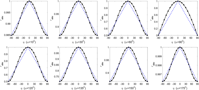
Figure 5: The curves of the unsigned tri-variate correlation coefficient against the angle $\eta$. The angle $\alpha$ is fixed with different values, and $\eta$ is $\angle$COC₀ in Figure 4.

5.  CONCLUSION

References

[1]
Stigler, S. M. (1989), “Francis Galton’s Account of the Invention
of Correlation,” Statistical Science, 4, 73–79.
[2]
Dragomir, S. S. (1999), “A Generalization of Grüss’s Inequality
in Inner Product Spaces and Applications,” Journal of Mathematical Analysis and Applications, 237, 74–82.
[3]
Garnett, J. C. M. (1919), “On Certain Independent Factors in Mental
Measurements,” Proceedings of the Royal Society of London,
Series A, 96, 91–111.
[4]
Zeng, J. (1993), “A Bijective Proof of Muir’s Identity and the
Cauchy-Binet Formula,” Linear Algebra and its Applications,
184, 79–82.
[5]
Leonov, V. P. and Shiryaev, A. N. (1959), “On a Method of
Calculation of Semi-Invariants,” Theory of Probability &
its applications, 4, 319–329.
[6]
Hasebe, T. and Saigo, H. (2011), “Joint Cumulants for Natural
Independence,” Electronic Communications in Probability,
16, 491–506.
[7]
Wang, J. and Zheng, N. (2013), “A Novel Fractal Image Compression
Scheme With Block Classification and Sorting Based on Pearson’s
Correlation Coefficient,” IEEE Transactions on Image
Processing, 22, 3690–3702.
[8]
Kutner, M. H., Nachtsheim, C. J., Neter, J., and Li, W. (2005),
“Applied Linear Statistical Models,” 5th edition, New York:
McGraw-Hill.
[9]
Barth, N. (1999), “The Gramian and k-Volume in n-Space: Some
Classical Results in Linear Algebra,” Journal of Young
Investigators, 2.