Total and Partial Fragmentation Cross-Section of 500 MeV/nucleon Carbon Ions on Different Target Materials

Abstract

By using an experimental setup based on thin and thick double-sided microstrip silicon detectors, it has been possible to identify the fragmentation products due to the interaction of very high energy primary ions on different targets. Here we report total and partial cross-sections measured at GSI (Gesellschaft für Schwerionenforschung), Darmstadt, for 500 MeV/n energy ${}^{12}C$ beam incident on water (in flasks), polyethylene, lucite, silicon carbide, graphite, aluminium, copper, iron, tin, tantalum and lead targets. The results are compared to the predictions of GEANT4 (v4.9.4) and FLUKA (v11.2) Monte Carlo simulation programs.

I Introduction

The nuclear interaction mechanism of carbon ions with nuclei represent a key point in the understanding of delivered dose in cancer therapy applications. The effect of fragmentation diminishes the number of primary ions delivered to the region under treatment and produces a tail of damaging ionisation beyond the Bragg peak. In addition, the trajectories of fragments may be sufficiently perturbed compared to that of the incident ion that they deposit a non-negligible dose outside the volume of tissue being treated. The nuclear fragmentation studies are of interest also for radiation effects community [1, 2] since both primary Galactic Cosmic Rays (GCR) or their secondaries may cause Single Event Effects (SEE) on electronics systems and instrumentations. Carbon ions are a significant component of the GCR and of Solar Particle Events (SPEs) (see for instance [3] for a review of models of the near-Earth space radiation environment) and they contribute to the dose delivered to astronauts as well as to SEE occurring in electronics on long duration space missions. The external environment is fairly well known, but when the incident radiation interacts with the spacecraft hull and internal materials, nuclear fragmentation modifies the external radiation field [4]. A recent exhaustive review on this subject are given in [5, 6, 7]. Both applications, cancer therapy dose and optimization of shielding materials for space explorations, require an accurate knowledge of the physics of the fragmentation process. In this work we measured the total charge-changing cross-sections and partial cross-sections for individual fragments produced by a 500 MeV/n carbon beam on eleven different target materials. The experimental results are compared to the predictions of GEANT4 [8, 9] and FLUKA [10, 11] Monte Carlo simulation programs.

II Experimental Setup

The detection system designed and assembled by MAPRad [15] at INFN (Istituto Nazionale di Fisica Nucleare) Perugia clean room facilities [16]. The experimental apparatus (see Fig. 1) used to perform the measurement is based on the double-sided microstrip silicon detector (DSSD) technology.

Our first test set consisted of five double-sided $300~{}\mu$m thin microstrip silicon detectors (DSSD300) of the same type used in the AMS02 experiment [17].

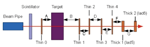
Figure 1: A general sketch of the setup: the position of Thin and Thick detectors

The implants on the two sides of DSSD300 run along orthogonal directions, providing X and Y measurements of ion impact position, with a readout pitch of 0.44 mm and external dimensions of 41x72x0.31 mm². The number of channels connectable to Front-End Electronics (FEE) is 160 + 96 for p and n side respectively however, on both sides, only central 96 channels were connected to FEE.

The second test set included two 1.5 mm thick microstrip silicon detectors (DSSD1500), produced by FBK of Trento (Italy), with 64 + 64 channels on p and n sides respectively. These sensors have a readout pitch of 0.5 mm and external dimensions of 35x35x1.5 mm² and all channels on both sides were connected to their respective FEE. The detectors mentioned above were arranged with the first (Thin0) and the second (Thin1) of the thin sensors, placed in fixed positions before and after the target, and were followed by the other three sensors (Thin2, Thin3, Thin4). The two thick sensors (Thick1, Thick2) were positioned as the last two sensors of the experimental setup. Fig. 1 shows a schematic drawing of the setup on the beam line for the ions.

The positions of Thin0 and Thin1 were chosen so that any target thickness among those available could be accomodated in between. The positions of the other sensors were varied during the experiment to assess the effect of geometrical acceptance on the final result. The value of the distances, measured with the laser device with resolution better than 0.1 mm, are show in Table I.

TABLE I: Distances (mm) between detectors in the different configurations in August 2010 session. For distances corresponding to each letter please refer to Fig. 1

Config.	A+B+Target	C	D	E	F	G
1	719.33	67.96	65.56	75.28	74.80	79.61
2	719.33	65.59	64.23	73.17	70.80	76.79
3	719.33	79.39	119.66	79.45	119.29	80.25
4	719.33	79.56	120.76	80.67	118.69	79.49

Although the sensors have self triggering capabilities, a plastic scintillator was inserted between the point where the beam is extracted in air and the experimental setup, to act as an external trigger for the data acquisition (DAQ) electronics. The setup was equipped with temperature sensors and with a cooling system, flowing air at $2\,^{\circ}{\rm C}$ on the surface of the detectors. Fig. 2 shows the experimental setup assembled at GSI.

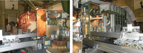
Figure 2: The photos show the detector setup at GSI

Testing took place in experimental Cave A at GSI-Darmstadt in August 2010. The beam was ${}^{12}C$ with an energy of 500 MeV/n. Beam intensity was about 5k to 10k counts per spill with a duration of 10s, according to GSI monitoring system. Several target materials were used: water (in flasks), polyethylene, aluminium, lucite, graphite, iron, tin, lead, copper, tantalum, silicon carbide. For some target types, several different thicknesses were used. The details are reported in Table II.

TABLE II: Tested target materials and relative thicknesses.

Material	Thickness $(g/cm^{2})$
air	0.035
water	5.700
lucite	3.840
polyethylene	0.465
silicon carb.	1.580
aluminium	5.450
graphite	1.734
graphite	3.434
copper	4.628
iron	3.935
iron	6.611
tin	3.655
tin	5.848
tantalum	3.330
tantalum	6.660
lead	3.689
lead	6.810

For each target we collected at least $10^{6}$ events. A set of data with no target was also taken to account for the contribution due to interaction in air or in the silicon sensor itself. Data with no target were also used to evaluate the corrections to be applied to data described in following sections.

III Data Processing

The data analysis consists of two main phases. During the first phase a preselection of events that were suitable for the analysis and evaluation of correction factors on raw charge signals collected in the sensors were carried out. The second phase includes the track fitting and particle identification procedures.

For each run, a set of data is collected by using random trigger (with no beam on) to calculate the pedestal and random noises of readout channels as well as the common mode noise which is the mean of the uniform shift over all channels of given readout chip. After random trigger data the beam was turned-on to collect the real beam data. The cluster formation, which is the group of adjacent strips collecting charge created by a traversing particle that survives several selection cuts were applied.

III-A Data Unfolding

The requests in this stage were mostly geared towards a general quality of the event and observed signals (clusters of neighbouring readout channels). For this purpose we considered only those events that are separated in arrival time with more than $100\mu$s from the previous.

The collected charge (Analog to Digital Converter (ADC) counts) on the several sensors has a noticeable dependence on the particle impact position and on the different sensors yield. Therefore corrections to these effects are needed for accurate identification of the fragmentation products.

III-A1 Gain Correction

Both sides of detectors were read-out through a VLSI (Very Large Scale Integration) [18] that consist into self-triggering, pre-amplifier, sample & hold, multiplexer circuitry with a dynamic range of $\pm$132 MIPs. The circuitry has internal calibration line for each of its 32 channels. All VA32TA3.2 were calibrated between few MIPS up to well above saturation levels by injecting, on bench, known values of charge load to trace for each channel the calibration curves. The gain responses of each channel of a given VA32TA3.2 were normalized to its average value. The same way, average gain of a given side of a given sensor was then calculated and single channel correction factors were finally determined.

III-A2 $\eta$ Correction

The parameter $\eta$ is defined using the two channels of a cluster that collected the highest signals as:

$$\eta=\frac{Q_{r}}{Q_{l}+Q_{r}}$$ (1)

where the subscripts “l” and “r” label the collected charge (Q) of the leftmost and rightmost of the two most highest strips respectively. An ion impinging close to a readout strip will yield a value of $\eta$ close to 0 or to 1, while ions hitting in the interstrip region will have $\eta$ close to 0.5. Due to the poor capacitive coupling towards the connected readout channels, the hits in the 0.5 region register a lower charge: while this is not a problem on Thin0, where we have only primary ions, it tends to mix the different populations of fragments in the subsequent sensors, so it is necessary to implement a correction factor depending on $\eta$ to normalize the collected charge to a common baseline. The correction factor for collected charge in a given $\eta$ bin is the same for all (primary and fragments), hence, the correction was evaluated using data from a run without target, then it as applied to all other samples.

III-A3 Sensor to Sensor Correction

A further correction was applied to the collected charge to account for the different yield of each sensor of the setup. Besides the obvious difference between thin and thick detectors, that implies different amplitude of the signals, each sensor DAQ combination has a different yield. The value of charge for primary particle peak from the various sensors can vary substantially, and this is also true for the charge produced by fragmentation products; in order to allow for a uniform treatment of data from different silicon sensors we fitted the main peaks of each sensor with a gaussian and used the ratio between the fit’s most probable values to scale the charge of thin sensors to a common base, which we chose to be the value of charge observed on Thin0. The correction factor was evaluated on a dataset without target and then applied to all other data sets.

III-B Track Fitting

Each sensor gives the X-Y impact position of the particles, while the Z coordinate is known a priori from the mounting position of the sensor.

The position identification capability of DSSD is used in the subsequent analysis, since it is to be expected that the ions that pass through the target without fragmentation, will produce a sequence of hits in the various sensors that lie on a path that is closer to a straight line. Therefore fitting the tracks to a straight line and imposing a cut on the quality of the fit helps to identify both the unchanged beam ions and the fragments. In addition, track fitting helps in rejecting events with low spatial correlation between signals, due to inefficiencies of the detectors, fluctuations in the measurements and signal pileup when a primary particle enters the set up during elaboration of signals.

To ensure that we can apply the track fitting, we checked that each sensor contains at least one signal on the p side; in case more than one cluster was present, we only consider the one with the highest charge. Since it is possible that a detector misses the particle for some inefficiency of the acquisition chain, the number of track points used in the fits can vary; in particular, it is possible for the track not to reach the last detector (Thick2) or, while still reaching it, to have missing intermediate points (holes). For our analysis we decided to consider only tracks with no holes, but since in principle a second interaction in the silicon sensors is possible, we allowed the track to be as short as two track points.

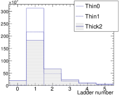
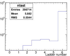
Figure 3: Left: distribution of the last detector with signal in a given track with no holes. Right: distribution of number of cluster per event per sensors Thin0, Thin1 and Thick2

Fig.  3 shows, on the right, that the distributions of the number of clusters for event is peaked at 1, even for the most distant sensor (Thick2). On the left side of the same Figure is shown the distribution of the last sensor with signal without having holes along the track. The majority of events reaches the last sensor, which, considering the small external dimensions of thick sensors, is consistent with the assumption that the fragments are mostly directed at low angles from the impinging ions momentum. Fig. 4 shows residuals between fitted track and actual hit positions on p-side for DSSD300 after the target.

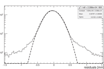
Figure 4: Residuals from the actual hit positions and fitted tracks for p-side of DSSD300 sensors after the target.

It is worth to notice that the mean value for the absolute residual of the fits after target is about $210\mu$m, that is very close to the value expected for a readout pitch like the one we are using.

All the necessary cluster information, as well as the quantities calculated in the track fitting procedure are stored in a file, that is the basis for the following step.

III-C Event Selection and Particle Identification

To distinguish between the primary ions and the products of the fragmentation, besides the track fitting results, we use charge information.

Fig. 5 shows the cluster charge correlation plots of the signals recorded on a pair of thin sensors (p sides). The plot refers to a pair of sensors (Thin1 and Thin2), but the same type of plot was produced for all other couples of sensors of the same kind.

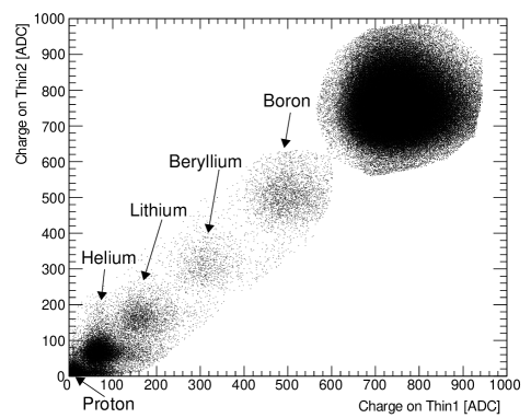
Figure 5: Scatter plot of charge observed in detector Thin2 versus detector Thin1. Along the diagonal are visible the populations due to primary ions and the fragmentation products.

We saw that every couple of sensors basically shows the same structure, with a series of approximately round areas aligned along the diagonal, which can easily be interpreted as the fragmentation products plus the primary peak. Events with charge signal out of diagonal may arise from a series of different reasons, such as inefficiencies in the detector’s charge collection. Such events was removed with a graphical cut. The application of the graphical cut yields a cropped scatter plot for each of the sensor combination mentioned above. From each one of these cropped plots we can obtain two collected charge spectra by projecting the points to one of the axes (Fig. 6). The vertical bands are representing one sigma limits around most probable charge values. For their use see LR(Z) calculation in next paragraph.

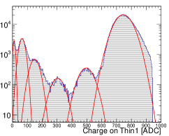
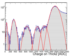
Figure 6: Collected charge spectra. The left plot refers to the first thins after the target, the right one to the last thick sensors. The relative positions of the peaks are compatible with the atomic number of the fragmentation products and the primary carbon beam.

In this analysis, in order to reduce the charge misidentification due to overlap in charge distributions, in spite of loss of statistics, we considered only the events wich falls within one sigma of the charge distribution peaks.

Fragments of different charge have different track fit quality, in particular, for low charge fragments, up to Li, fit quality is worse possibly because in their case, fragment multiplicity increases, leading to a mixing of tracks and degraded fitting performance. By selecting the events that are close to the peaks in the various charge spectra, we observed that the higher the charge released in the sensors, the smaller the deviation from the primary ion trajectory and the better is the fit quality (Fig. 7).

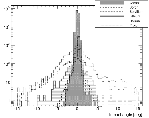
Figure 7: Angles as evaluated by track fitting procedure for different charge populations. Low Z ions scatter off the target at higher angles.

A charge dependent cut on the Chi-square fit probability has been applied: we required a fit probability greater than 0.9 for events with ADC counts more than 500, a fit probability greater than 0.8 for events with falling in the interval between 250 and 500 ADC counts and no cut on fit probability for events with less than 250 ADC counts.

This analysis procedure allows to obtain a set of fitted peak functions for each sensor. Such sets of function can be used to implement a Likelihood test. To this purpose we used the fitted parametrisation $f_{Z_{S}}(x)$ as a function of the value of charge for a given fragment species of charge Z and measured on a given sensor S, to define a normalised probability density function:

$$P_{Z_{S}}(x)=\frac{f_{Z_{S}}(x)}{\int f_{Z_{S}}(x)dx}$$ (2)

For each event, we can combine the probability that signal of amplitude $x_{S}$ from sensor S to be the effect of ion Z by multiplying them. We define the LogLikelihood that an event is due to ion of atomic number Z as:

$$L(Z)=-\sum{log(f_{Z_{S}}(x_{s}))}$$ (3)

We can then compute at each event the Likelihood for the various Z values and choose the most suitable. To perform the identification we define a test quantity:

$$LR(Z)=\frac{L(Z)}{L(Z)+L(Z-1)}$$ (4)

Here LR(Z) stands for Likelihood Ratio: this test is specifically targeted at the discrimination of one peak from the ones with Z differing by one unit, since the major contribution to wrong charge assignments are essentially coming from neighbouring peaks. To study the capability of the test to identify the ions we performed a very strict selection, containing only the events whose collected charge was within one sigma of the same peak in Thin0 and Thin4 and considered them as “pure samples”. In this way we can evaluate the LR(Z) with a fairly accurate a priori knowledge of the real ion specie and see if it is identified as such.

In Fig. 8 we plotted LR(Z) and LR(Z+1) for the six “pure samples”, identified by different gray tones, under two Z hypothesis, namely Z=2 and Z=3. Given our definition of LR, we expect to observe both a low LR(Z) and a high LR(Z+1) for the sample that really corresponds to the hypothesis. In fact, we see that the population whose Z is the hypothesis shows to the left of the value 0.5 in both plots (Z=2 line on the left plot, Z=3 line on the right plot) so accepting those ions with LR(Z=2) $<$ c1, with c1 $<$ 0.5, we are selecting the Helium with contamination from Li and Be, however, asking that LR(Z=3) $>$ c2, with c2 $>$ 0.5 we reject the Li and Be population (right plot Fig. 8). The actual test becomes a series of comparisons, where the event is assigned to one value of Z if

$$LR(Z)<c_{1};c_{1}\leq 0.48~{}~{}~{}~{}~{}~{}~{}~{}LR(Z+1)>c_{2};c_{2}\geq 0.53\\$$ (5)

The values for c1 and c2 were chosen looking at the “pure samples” from a set of data, then we used the same values for all other targets.

The selection efficiency of the criterion, as well as the contamination from misenterpreted ions were estimated. To this purpose, we defined the efficiency and contamination as

$$Eff_{Z}=\frac{\int_{X_{c1}(Z)}^{X_{c2}(Z)}{f_{Z}(x)dx}}{\int_{-\infty}^{+\infty}{f_{z}(x)dx}}$$ (6)

$$Cont_{Z,C}=\frac{\int_{X_{c1}(Z)}^{X_{c2}(Z)}{f_{C}(x)dx}}{\sum_{k}\int{f_{K}(x)dx}}$$ (7)

where the integrals at numerator are over the charge domain that would be selected by our acceptance criterion for a specific value of Z. The efficiency is the fraction of ions of charge Z that are accepted by the selection criterion, the contamination is defined as the fraction of particles identified as charge Z that is statistically expected to be misinterpreted particle of charge C.

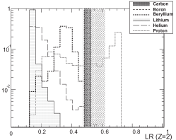
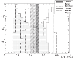
Figure 8: Likelihood ratio distribution for six pure sample of ions: On the left LR is evaluated assuming Z=2, on the right assuming Z=3.

IV Total charge-changing cross-section and partial fragmentation cross-section

After the described analysis procedure we obtain a set of numbers $N(Z)$ that represent the quantity of events where the highest charge in the event were identified as one specific specie of atomic number $Z$. Given the $N(Z)$ quantities, we define

$$P(Z)=\frac{N(Z)}{\sum N(Z)}$$ (8)

Data taken without a target are used to determine the background for each fragment Z. We define

$$P_{0}(Z)=\frac{N_{0}(Z)}{\sum N_{0}(Z)}$$ (9)

which refers to the results obtained with air only.

The total charge-changing cross-section for a given target of depth $d$ can be written

$$\sigma_{cc}=-\frac{Alog(P_{corr}(Z_{p}))}{\rho dN_{A}}$$ (10)

where $N_{A}$ is the Avogrado number, $\rho$ the target density, $A$ the target mass number, $Z_{p}$ the atomic number of the primary ions from the beam and

$$P_{corr}(Z_{p})=\frac{P(Z_{p})}{P_{0}(Z_{p})}$$ (11)

The error on $\sigma_{cc}$ is given by

$$\frac{\delta\sigma_{cc}}{\sigma_{cc}}=-\frac{\delta P_{corr}(Z_{p})}{P_{corr}(Z_{p})log(P_{corr}(Z_{p}))}$$ (12)

Partial fragment production cross-sections are given by

$$\sigma_{Z}=\sigma_{cc}\frac{P_{corr}(Z)}{1-P_{corr}(Z_{p})}$$ (13)

In order to derive the cross-section results we considered that a small fraction of the produced fragments can be out of geometrical acceptance of the detector, especially for low Z fragments which have the highest transverse momentum.

In addition, in any target, there is a finite probability for secondary interactions involving fragments. While these have no effect on the determination of the total cross-section, they affect fragment yield enhancing the number of lighter fragments. In order to estimate both the effects of geometrical acceptance and the fragment reinteractions Monte Carlo simulation of the full experimental setup were performed with GEANT4 and FLUKA. For this purpose we have developed a PYTHON based simulation framework that uses FLUKA and/or GEANT4 for the run of the Monte Carlo simulations and offer a common set of simple functions for the definition of the beam, of the geometry, and for the post-processing analysis. For the GEANT4 simulations the geometry of the different experimental setup were defined in form of Geometry Data Markup Language (GDML) files. These GDML files were translated into FLUKA geometry input cards by a PYTHON GDML-to-FLUKA geometry translator developed by us. Fig. 9 represents the modeling of one of the experimental set-up considered in this project as seen in GEANT4 (left) and in FLUKA (right) visualisation drivers. The PYTHON interface we have developed was to avoid any error which may have been introduced by entering into the FLUKA the parameters of a complex geometry, as in this work, via data cards. The interface takes simply the parameters set from GDML description and converts it to FLUKA data card readable values. Therefore, existing codes such as MRED [12] and others [13, 14] more complicated than ours and they point to solve higher order problems.

Large Monte Carlo samples of different experimental configurations tested at GSI were produced and analysed. The geometrical inefficiencies were then evaluated and the cross-section values were corrected accordingly. The cross-sections determined for several thicknesses and of same material and for several experimental configurations have been combined to enhance the statistical accuracy of the measurements.

The error on total cross-section includes both statistical and systematic contributions. Main contributions to systematic error originate from two effects: one is the difference in cross-sections obtained by using different target thickness of the same material and different experimental configurations, the other is the geometrical acceptance calculations obtained by Monte Carlo runs using different physics lists produce different fragment angular distributions (see Fig. 13). The overall contribution gives a systematic uncertainty of about $3\%$.

The fragment production cross-section is proportional to the total charge-changing cross-section (eq. 13), therefore any systematic error in the latter propagates to systematic error in the former. In addition systematic errors due to ambiguous cases where there is an inefficiency in charge assignment procedure have been evaluated and accounted for.

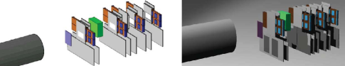
Figure 9: Visualisation in GEANT4 (left) and FLUKA (right) of the geometrical modeling of experimental setup used in this work.

The summary of the measurements on all tested target materials,together with literature data, are reported in Table III. In Table IV the partial fragment production ratio with respect to the total charge-changing cross-section for all tested target materials are listed.

TABLE III: Total charge-changing cross-section: comparison with previous measurements. The numbers in the fourth column are the relative errors (in %) referring to calculated values for this experiment or to data from literature.

Energy (MeV/n)	Target	Cross-Section (mbarn)	Rel. Error (%)	Ref.
200	graphite	658 (7)	1.1	[25]
267	graphite	748 (19)	2.5	[26]
290	graphite	706 (7)	1.0	[27]
400	graphite	672 (7)	1.0	[25]
400	graphite	713 (11)	1.5	[29]
498	graphite	758 (15)	2.0	[26]
500	graphite	703 (18)	2.5	This exp.
192	aluminium	1179 (29)	2.5	[26]
267	aluminium	1078 (17)	1.6	[26]
290	aluminium	1155 (108)	9.3	[27]
290	aluminium	1052 (11)	1.0	[29]
400	aluminium	1011 (9)	0.9	[29]
498	aluminium	1103 (28)	2.5	[26]
500	aluminium	1095 (26)	2.5	This exp.
676	aluminium	1096 (100)	9.1	[26]
500	iron	1509 (37)	2.5	This exp.
290	copper	1625 (18)	1.1	[29]
400	copper	1557 (10)	0.6	[29]
500	copper	1598 (50)	3.1	This exp.
290	tin	2069 (18)	0.9	[29]
400	tin	2035 (21)	1.0	[29]
500	tin	2141 (79)	4.9	This exp.
500	tantalum	2936 (105)	3.6	This exp.
290	lead	2795 (15)	0.5	[29]
400	lead	2745 (45)	1.6	[29]
500	lead	2926 (116)	3.9	This exp.
192	water	1264 (16)	1.3	[26]
267	water	1163 (13)	1.1	[26]
326	water	1250 (51)	4.1	[30]
352	water	1202 (47)	3.9	[30]
377	water	1253 (45)	3.6	[30]
498	water	1220 (20)	1.6	[26]
500	water	1211 (27)	2.2	This exp.
670	water	1261 (13)	1.0	[26]
192	lucite	7250 (102)	1.4	[26]
267	lucite	6733 (74)	1.1	[26]
464	lucite	7019 (112)	1.6	[26]
500	lucite	7051 (165)	2.3	This exp.
676	lucite	7170 (360)	5.0	[26]
192	polyethylene	1157 (13)	1.1	[26]
267	polyethylene	1075 (11)	1.0	[26]
498	polyethylene	1135 (15)	1.3	[26]
500	polyethylene	1120 (54)	7.0	This exp.
500	silicon carb.	1974 (91)	4.9	This exp.

TABLE IV: Ratio of partial fragmentation cross-section over total charge-changing cross-section for ${}^{12}C$ ion at 500 MeV/n energy for all tested target materials.

Target	$Z=5$	$Z=4$	$Z=3$	$Z=2$	$Z=1$
graphite	10.9 (0.6)	6.3 (0.4)	11.9 (1.5)	56.9 (2.8)	14.1 (1.4)
aluminium	9.7 (0.5)	5.0 (0.3)	9.2 (1.2)	55.7 (3.4)	20.3 (1.9)
iron	8.3 (0.4)	4.2 (0.3)	10.0 (1.2)	52.2 (3.5)	25.2 (2.1)
copper	8.7 (0.8)	5.8 (0.6)	8.7 (2.2)	50.8 (5.8)	26.0 (4.4)
tin	7.1 (0.6)	4.5 (0.5)	7.9 (1.4)	50.3 (4.8)	30.2 (3.3)
tantalum	6.5 (0.5)	3.8 (0.4)	7.3 (0.9)	49.3 (3.2)	33.1 (2.4)
lead	7.0 (0.7)	4.0 (0.5)	6.6 (1.2)	48.6 (4.2)	33.9 (3.2)
water	13.9 (0.5)	6.1 (0.3)	13.3 (2.0)	56.4 (4.0)	10.4 (1.7)
lucite	13.3 (0.5)	6.5 (0.3)	12.1 (2.0)	56.7 (4.3)	11.5 (1.5)
polyethylene	13.3 (1.6)	5.3 (0.9)	11.5 (1.9)	60.4 (5.7)	9.4 (1.6)
silicon carb.	9.2 (1.3)	6.1 (1.0)	10.2 (2.6)	57.1 (7.2)	17.4 (3.1)

V Comparison of results with GEANT4 and FLUKA simulations

The measured total charge-changing cross-sections has been compared with the predictions provided by nuclear ion-ion interaction models implemented in FLUKA and GEANT4 simulation tools (Fig. 10). Except for Abrasion and Ablation models there is an agreement within 10% between simulation and data for all targets. For several targets FLUKA shows an agreement with data within 3-5%.

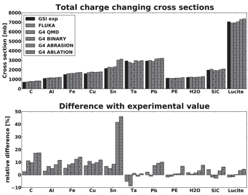
Figure 10: Total charge-changing cross-section for 500 MeV/n ${}^{12}C$ ion as a function of target type, compared with different physics models of GEANT4 and FLUKA. The bottom panel represents the relative differences between the model and the experimental cross-section.

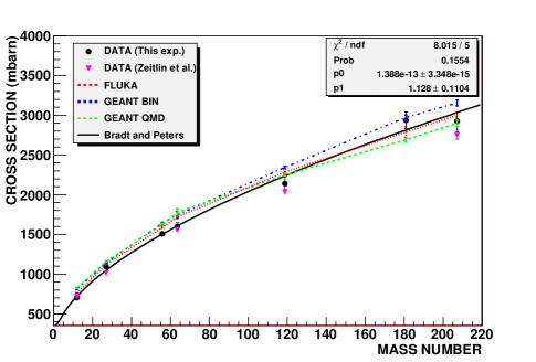
Figure 11: Experimental total charge-changing cross-sections measured in this experiment for elemental target as a function of target mass number $A$. In the plot model predictions from GEANT4 and FLUKA togheter with the measurement given in [29] are reported. The solid line is the fit to data as measured in this work with the Bradt and Peters curve.

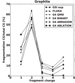
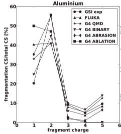
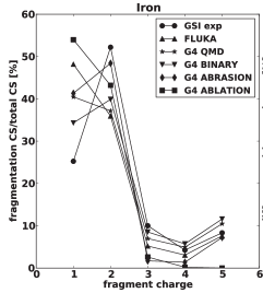
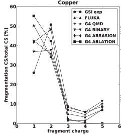
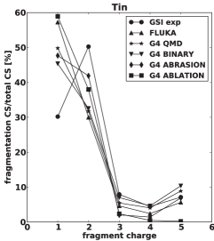
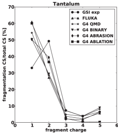
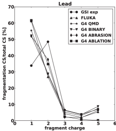
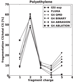
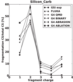
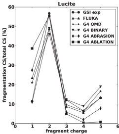
Figure 12: Measured ratio of fragmentation cross-section over total charge-changing cross-sections for ${}^{12}C$ ion at the energy of 500 MeV/n interacting with different targets compared with different physics models of GEANT4 and FLUKA.

Fig. 11 shows the variation of total charge-changing cross-sections as a function of target mass number $A$ for elemental targets. Data have been fitted with the simple geometric cross-section model calculation based on Bradt and Peters [22] parametrisation

$$\sigma(A_{p},A_{t})=\pi r_{0}^{2}\big{(}A_{p}^{1/3}+A_{t}^{1/3}-b\big{)}^{2}$$ (14)

where $A_{p}$ and $A_{t}$ are the mass number of the projectile and target, respectively. The results of the fit gives the values $r_{0}=1.39\pm 0.03$ and $b=1.13\pm 0.11$ to be compared with the values of $r_{0}=1.29$ and $b=0.86$ as in [29] and $r_{0}=1.35$ and $b=0.83$ as in [23].

Fig. 12 shows the ratio of fragmentation cross-sections over the total charge-changing cross-sections for different target materials, for GEANT4 models, FLUKA and experimental data. On the x axis the fragment charge refers to the charge number Z of the heaviest fragment. For Z$\geq$3 the G4QMD, G4 Binary and FLUKA models agree reasonably well with this experiment. For $Z=2$ (only He and H isotopes are produced) and Z=1 (only H isotope is produced), the Monte Carlo models show larger discrepancies compared to the experimental data. In general the models under-estimate the fragmentation cross-section for Z=2 and over-estimate it for Z=1. In addition the discrepancy is higher for high mass number targets with respect to low mass number targets.

From the track fitting of the experimental data the angle $\Theta$ between the beam-line direction and the XZ projection of the direction of the highest-Z fragment after the target, can be deduced. In Fig. 13 the angular distribution is shown for fragment events in water target and compared with Monte Carlo models.

VI Conclusions

We measured at GSI, Darmstadt, the total charge-changing and partial fragment cross-sections for the interactions of ${}^{12}C$ at 500 MeV/n on several targets.

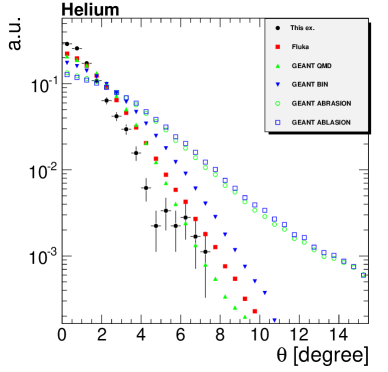
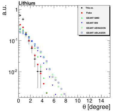
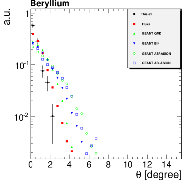
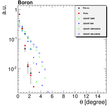
Figure 13: Angular distribution of fragments events produced in the interaction of 500 MeV/n ${}^{12}C$ ions on water target compared with different physics models of GEANT4 and FLUKA: Helium (top left), Lithium (top right), Beryllium (bottom left), Boron (bottom right).

A PYTHON based simulation framework has been developed to simulate with GEANT4 and FLUKA the interaction of the ${}^{12}C$ beam with the different experimental setups considered in this study. The comparison of measured data with the simulation models gives a reasonable agreement for total charge-changing cross-sections. The detailed analysis of ${}^{12}C$ data has shown that there is a discrepancy between Monte Carlo model predictions and data on low Z (Z=1 and Z=2) cross-section values for almost all target materials. The discrepancy is systematic such that the data sees more Z=2 particles (higher partial cross-section) than Z=1 ones with respect to the expectations of both FLUKA and GEANT4.

Further studies have been performed to investigate if the origin of .such a discrepancy between Monte Carlo and data is due to some instrumental effect of our experimental setup. If the fragmentation products can hits the DSSDs within few mm an overlap between charge clusters may occurr leading to misidentified products. Since a typical proton cluster is 2.5 strips (about 1mm) wide, if three or more protons hits the detector within 1.5-2 mm the total product charge can be confused with that of a helium.

To establish the frequency of occurrence of this, we performed MC simulations and we seen that, depending on target material, a fraction going from 1.5% to 5% of total Z=1 events, at least three protons, in 1.5 mm, may overlap to mimic a helium cluster in Thin1. The fraction variation depends on target mass and it is lowest for graphite and highest for lead. This effect has been included in systematic uncertainties and, taking also into account of the reasonable agreement in the fragment angular distribution shown in Fig. 13, does not allow to explain the discrepancies between MC and data we observed in Z=2 and Z=1 events.

Differences on cross-section values calculated by using different Monte Carlo codes and physics lists are also remarkable. Here it is important to recall that the partial cross-section both in data analysis and in Monte Carlo are calculated by using the highest charge in a given event. In other words, the partial cross-sections of Z=2 are coming from events containing 3 Helium or 2 Helium and 2 protons or 1 Helium and 4 protons. Naturally, partial cross-section of Z=1 particles are deriving from 6 proton events only. In order to confirm or reject the above mentioned discrepancies further studies using an experimental setup with improved Z=1 and Z=2 separation capability may be of help.

References

- [1] M. A. Clemens, N. A. Dodds, R. A. Weller, M. H. Mendenhall, R. A. Reed, R. D. Schrimpf, T. Koi, D. H. Wright, and M. Asai, ”The Effects of Nuclear Fragmentation Models on Single Event Effect Prediction,” IEEE Trans. Nucl. Sci., vol. 56, no. 6, pp. 3158-3164, Dec. 2009.
- [2] M. S. Sabra, R. A. Weller, M. H. Mendenhall, R. A. Reed, M. A. Clemens, and A. F. Barghouty, ”Validation of Nuclear Reaction Codes for Proton-Induced Radiation Effects: The Case for CEM03,” IEEE Trans. Nucl. Sci., vol. 58, no. 6, pp. 3134-3138, Dec. 2011.
- [3] M. A. Xapsos, P. M. O’Neill, and T. P. O’Brien, ”Near-Earth Space Radiation Models,” IEEE Trans. Nucl. Sci., vol. 60, no. 3, pp. 1691-1705, June 2013.
- [4] J. W. Wilson et al., ”Shielding Strategies for Human Space Exploration,” NASA Conference Publication 3360, Dec 1997.
- [5] M. Durante, F. A. Cucinotta, ”Physical basis of radiation protection in space travel,” Reviews of Mod. Phys. 83, Oct-Dec 2011.
- [6] M. Silvestri, E. Tracino, M. Briccarello, M. Belluco, R. Destefanis, C. Lobascio, M. Durante, G. Santin, and R. D. Schrimpf, ”Impact of Spacecraft-Shell Composition on 1 GeV/Nucleon 56Fe Ion-Fragmentation and Dose Reduction,” IEEE Trans. Nucl. Sci., vol. 58, no. 6, pp. 3126-3133, Dec. 2011.
- [7] M. Silvestri, E. Tracino, R. Destefanis, C. Lobascio, G. Santin, and P. Calvel, ”Influence of Spacecraft Shielding Structures on Galactic Cosmic Ray-Induced Soft Error Rate,” IEEE Trans. Nucl. Sci., vol. 59, no. 4, pp. 1078-1085, Aug. 2012.
- [8] S. Agostinelli et al, GEANT4 Coll. ”GEANT4 a simulation toolkit,” Nucl. Instr. and Meth. A 506 (2003) 250-303.
- [9] J. Allison et al, GEANT4 Coll. ”GEANT4 developments and applications,” IEEE Trans. on Nucl. Sci, 53 (2006) 270-278.
- [10] G. Battistoni et al, ”The FLUKA code: Description and bench-marking,” Proceedings of the Hadronic Shower Simulation Workshop, Sep 2006, AIP Conference proceedings, 896 (2007) 31-49.
- [11] A. Fasso et al, GEANT4 Coll. ”FLUKA: a multi-particle transport code,” CERN-2005-10, INFN/TC 0511, SLAC-R-773, 2006.
- [12] R. A. Weller, M. H. Mendenhall, R. A. Reed, R. D. Schrimpf, K. M. Warren, B. D. Sierawski, and L. W. Massengill, “Monte Carlo Simulation of Single Event Effects,” IEEE Trans. Nucl. Sci., vol. 57, no. 4, pp. 1726-1746, Aug. 2010.
- [13] S. Uznanski, G. Gasiot, P. Roche, C. Tavernier, and J. L. Autran, “Single Event Upset and Multiple Cell Upset Modeling in Commercial Bulk 65-nm CMOS SRAMs and Flip-Flops,” IEEE Trans. Nucl. Sci., vol. 57, no. 4, pp. 1876-1883, Aug. 2010.
- [14] G. Hubert, S. Duzellier, C. Inguimbert, C. Boatella-Polo, F. Bezerra, and R. Ecoffet, “Operational SER calculations on the SAC-C orbit using the multi-scales single event phenomena predictive platform (MUSCA SEP3),” IEEE Trans. Nucl. Sci., vol. 56, no. 6, pp. 3032-3042, Dec. 2009.
- [15] MAPRad s.r.l., Via Cristoforo Colombo 19/I; Perugia (Italy), website: http://www.maprad.com
- [16] Clean Room Facility, INFN Perugia, http://www.pg.infn.it/sez/laboratorihome.htm
- [17] B. Alpat et al, ”Charge determination of nuclei with AMS-02 silicon tracker,” Nucl. Instr. and Meth. in Phys. Res. A 540 (2005) 121-130.
- [18] Ideas, Va32Ta3.2 manual (ver. 0.95), Jan 2003.
- [19] La Tessa et al, ”Fragmentation of 1 GeV/nucleon iron ions on thick targets relevant for space explorations,” Advances in Space Research 35 (2005) 223-229.
- [20] C. Zeitlin et al, ”Heavy fragment production cross-sections from 1.05 GeV/nucleon 56Fe in C, Al, Cu, Pb and CH2 targets,” Nucl. Phys. C 56 (1997) 388.
- [21] L. W. Townsend and J. W. Wilson, Radiat. Res. 106, 283 (1986).
- [22] H.C. Bradt and B. Peters, Phys. Rev. 77, 54 (1950)
- [23] C. X. Chen et al, Phys. Rev. C 49, 3200 (1994)
- [24] H. Dekhissi et al, Nucl. Phys. A662, (2000), 207
- [25] W.R. Weber et al, ”Individual charge-changing fragmentation cross-section of relativistic nuclei in hydrogenum, helium and carbon targets,” Phys. Rev. C 41 (1990)
- [26] I. Schall et al, ”Charge-changing nuclear reactions of relativistic light-ion beams (5¡=Z¡=10) passing through thick absorbers,” Nucl. Instr. and Meth. B 117 (1996), 221-234.
- [27] S. Cecchini et al, ”Fragmentation cross-section of Fe56+, Si14+ and C6+ ions of 0.3-10 A GeV on polyethylene CR39 and aluminium targets,” Radiation Measurements 44 (2009) 853-856.
- [28] A. N. Golovchenko et al, ”Fragmentation of 200 and 244 MeV/u carbon beams in thick tissue-like absorber,” Nucl. Instr. and Meth. B 159 (1999) 233-240. 853-856.
- [29] C. Zeitlin et al, ”Fragmentation Cross-section of 290 and 400 MeV/nucleon 12 C Beams on Elemental Targets,” Phys. Rev, C 76, 014911 (2007).
- [30] T. Toshito et al, ”Measurements of total and partial charge-changing cross-section for 200-400 MeV/nucleon in water and polycarbonate,” Phys. Rev. C 75, 054606 (2007).