A distance on curves modulo rigid transformations

Abstract

We propose a geometric method for quantifying the difference between parametrized curves in Euclidean space by introducing a distance function on the space of parametrized curves up to rigid transformations (rotations and translations). Given two curves, the distance between them is defined as the infimum of an energy functional which, roughly speaking, measures the extent to which the jet field of the first curve needs to be rotated to match up with the jet field of the second curve. We show that this energy functional attains a global minimum on the appropriate function space, and we derive a set of first-order ODEs for the minimizer.

MSC classification: 58E30 (Primary), 49Q10, 53A04 (Secondary).

1 Introduction

In this paper, we establish a new, geometric method for quantifying the difference between curves in Euclidean space, based on the amount of deformation needed to optimally match the jets of two curves.

In a nutshell, our method can be described as follows. Given two curves $c_{1},c_{2}$ defined on the same interval $I$, and with values in $\mathbb{R}^{n}$, we try to rotate the tangent vector field of $c_{1}$ as well as possible into that of $c_{2}$. As a first attempt, we may therefore look for a family $g(s)\in O(n)$ of orthogonal transformations, so that

$$g(s)c_{1}^{\prime}(s)=c_{2}^{\prime}(s)\quad\text{for all $s\in I$},$$ (1)

and quantify the distance between $c_{1}$ and $c_{2}$ as the “magnitude” of $g(s)$ in some appropriate sense. The hard constraint (1) cannot generally be satisfied, however, since $O(n)$ preserves lengths. Therefore, we relax it into a soft constraint and look instead for a curve $g(s)$ which satisfies (1) approximately, while at the same time trying to minimize its variation. One way of doing so is by considering a functional of the form

$$E[g;c_{1},c_{2}]=\int_{I}\left(\lVert g(s)c_{1}^{\prime}(s)-c_{2}^{\prime}(s)\rVert^{2}+\lVert g(s)^{-1}g^{\prime}(s)\rVert^{2}\right){\;\textrm{d}}{s},$$ (2)

where $s\mapsto g(s)$ are curves in $O(n)$. The distance between $c_{1}$ and $c_{2}$ we then define as the infimum of $E$ over all possible curves $g(s)$:

$$d(c_{1},c_{2})=\inf_{g}E[g;c_{1},c_{2}].$$

Theorem 3.2 shows that this notion indeed defines a distance, on the quotient space $C^{k}(I,\mathbb{R}^{n})/E(n)$ of $k$-times differentiable curves modulo rotations and translations. That is, if $c_{2}$ can be obtained from $c_{1}$ by a rigid isometry, then the distance vanishes. Conversely, if the distance is nonzero, then the curves are not related by a rigid isometry. More generally, the distance function $d(c_{1},c_{2})$ is invariant (in both arguments separately) under the action of the Euclidean group $E(n)$ on the space of curves.

A similar energy functional was considered in [HNV13] and we employ a similar variational approach to characterize the minimizer $g(s)$. However, whereas [HNV13] considered the action of the Euclidean group $E(n)$ directly on the curves itself, we use instead the action of the orthogonal group $O(n)$ on the tangent vector field and the higher derivatives. The result is a notion of (dis)similarity between curves which is a true distance function, i.e. which is symmetric, non-negative, and satisfies the triangle inequality. Furthermore, we prove that the energy functional $E$ attains its minimum in the space of curves $H^{1}(I,O(n))$, and that a minimizer $g$ satisfies the variational equations in the strong sense, so in particular $g\in C^{2}(I,O(n))$.

Plan of the paper

In section 3 we first define a slight generalization of (2), in which not just the tangent vector field of $c_{1},c_{2}$ but also higher-order derivatives (i.e. jets of $c_{1},c_{2}$) are taken into account, and in section 4 we derive a set of variational equations which characterize critical points of the energy and provide some examples in section 5. In section 6 we prove existence of minimizers of $E$, and we show that any such minimizer must necessarily be a solution of the variational equations. We finish the paper by giving a probabilistic interpretation in section 7 for the curve matching energy functional.

2 Geometric Preliminaries

2.1 Spaces of jets and their duals

We consider a given parametrized curve $c\colon I\to\mathbb{R}^{n}$ with $I$ a bounded, closed interval and we denote by $j^{1,k}c$ the $(1,k)$-jet of this curve. By definition,

$$(j^{1,k}_{s}c)(\sigma)=\sum_{i=1}^{k}\frac{1}{i!}\frac{d^{i}c}{ds^{i}}(s)(\sigma-s)^{i},$$

which is simply the $k$-th order Taylor expansion at the point $s\in I$ without the zeroth order term. For each $s$ we may view $j^{1,k}_{s}c$ as an $n\times k$-matrix, whose $i$-th column is the $i$-th derivative of $c$ evaluated at $s$:

$$j^{1,k}_{s}c=\begin{pmatrix}\vline&&\vline\\ c^{\prime}(s)&\cdots&c^{(k)}(s)\\ \vline&&\vline\end{pmatrix}.$$

We let $V$ be the vector space of $n\times k$-matrices, so that $j^{1,k}c$ can be viewed as a parametrized curve on the interval $I$ with values in $V$. For future reference, we identify the dual $V^{\ast}$ with $V$ itself by means of the (Frobenius) inner product

$$\langle A,B\rangle_{V}=\operatorname{tr}(A^{T}B),$$

for $A,B\in V\cong V^{\ast}$. Secondly, we endow $V$ itself with a weighted inner product, defined as follows. For constants $\lambda_{i}>0$, $i=1,\ldots,k$, we let

$$\langle A,B\rangle_{L}=\sum_{i=1}^{k}\sum_{j=1}^{n}\lambda_{i}A_{ji}B_{ji}=\sum_{i=1}^{k}\lambda_{i}\langle a^{(i)},b^{(i)}\rangle=\operatorname{tr}(LA^{T}B),$$ (3)

where $L$ is the diagonal matrix with entries $L_{ii}=\lambda_{i}$, $i=1,\ldots,k$, while $a^{(i)}$ and $b^{(i)}$, $i=1,\ldots,k$, are the columns of $A$ resp. $B$. We denote the norm induced by the inner product (3) by $\lVert\,\cdot\,\rVert_{L}$, and the induced flat operation by $\flat\colon V\to V^{\ast}$, which is given by $A\mapsto AL$.

2.2 The action of the orthogonal group on the space of jets

The Euclidean group $E(n):=O(n)\ltimes\mathbb{R}^{n}$ acts point-wise by rotations and translations on curves in $\mathbb{R}^{n}$ and induces an action by its subgroup $O(n)$ on the $(1,k)$-jets of these curves, in the following way. Let $c\colon I\to\mathbb{R}^{n}$ be a curve and consider an element $(g,x)$ of the Euclidean group $E(n)$. By point-wise multiplication, we obtain a transformed curve, $d$, defined by $d(s):=gc(s)+x$, for all $s\in I$. Note that the derivatives of $d$ are given by $d^{(i)}(s)=gc^{(i)}(s)$. In other words, the translational part of the action drops out, and we are left with an action of $O(n)$ on the jet space $V\cong J^{1,k}(\mathbb{R}^{n})$, given by

$$g\cdot A=\begin{pmatrix}\vline&&\vline\\ ga^{(1)}&\ldots&ga^{(k)}\\ \vline&&\vline\end{pmatrix}=gA,$$

where the operation on the right-hand side is simply matrix multiplication, and the $a^{(i)}$ are the columns of $A$.

The family of norms $\lVert\,\cdot\,\rVert_{L}$ which we introduced previously is natural in the sense that (for each set of constants $\lambda_{i}$), the norm $\lVert\,\cdot\,\rVert_{L}$ is invariant under the action of $O(n)$. This is clear from the expression (3), where the inner product $\langle\,\cdot\,,\,\cdot\,\rangle_{L}$ is expressed as a linear combination of the Euclidean inner products on each of the $k$ derivatives of the curve, each of which is individually $O(n)$-invariant.

We recall that the Lie algebra $\mathfrak{o}(n)$ of the orthogonal group consists of all antisymmetric $n\times n$-matrices $\Omega$, equipped with the Lie bracket $[\Omega,\Omega^{\prime}]=\Omega\Omega^{\prime}-\Omega^{\prime}\Omega$. The infinitesimal action of $\mathfrak{o}(n)$ on $V$ is given again by left matrix multiplication: any $\Omega\in\mathfrak{o}(n)$ defines a linear transformation on $V$ given by mapping $A\in V$ to $\Omega A$. The Lie algebra $\mathfrak{o}(n)$ is equipped with a positive-definite inner product defined by

$$\langle\Omega,\Omega^{\prime}\rangle_{\mathfrak{o}(n)}:=\operatorname{tr}(\Omega^{T}\,\Omega^{\prime})=-\operatorname{tr}(\Omega\,\Omega^{\prime})$$ (4)

and we use this inner product to identify the dual space $\mathfrak{o}(n)^{\ast}$ with $\mathfrak{o}(n)$ itself via matrix transposition.

2.3 The momentum map

The action of a Lie group $G$ on a manifold $M$ induces a (cotangent lift) momentum map $J\colon\mathrm{T}^{\ast}M\to\mathfrak{g}^{\ast}$. In our case, where $G=O(n)$ acts by linear transformations on the vector space $V$, we find that $J$ is a bilinear map, and denote it by the diamond operator, $\diamond\colon V\times V^{\ast}\to\mathfrak{g}^{\ast}$. To ease later notation, let $\flat\colon V\to V^{\ast}$ denote the identification of dual spaces induced by $\langle\,\cdot\,,\,\cdot\,\rangle_{L}$. Then, for each $A,B\in V$, $A\diamond B^{\flat}$ is an element of $\mathfrak{o}(n)^{\ast}$, defined by

$$\langle A\diamond B^{\flat},\Omega\rangle_{\mathfrak{o}(n)^{\ast}\times\mathfrak{o}(n)}=\langle B^{\flat},\Omega A\rangle_{V^{\ast}\times V}$$ (5)

for all $\Omega\in\mathfrak{o}(n)$. Using the expressions (3) and (4) for the inner products, we may rewrite this definition as

$$\operatorname{tr}((A\diamond B^{\flat})\Omega)=\operatorname{tr}((LB^{T})(\Omega A))=\operatorname{tr}(ALB^{T}\Omega),$$

and as this must hold for all $\Omega\in\mathfrak{o}(n)$, we have that

$$A\diamond B^{\flat}=(ALB^{T})_{\mathrm{antisymm}}=\frac{1}{2}(ALB^{T}-BLA^{T}).$$ (6)

From the previous expression, or by direct inspection, it is easy to derive the following result.

Lemma 2.1.

The diamond operator (5) composed with the flat operator is antisymmetric, viz. $A\diamond B^{\flat}=-B\diamond A^{\flat}$ for all $A,B\in V$.

3 The curve registration functional

Given a source and target curve $c_{1},c_{2}\colon I\to\mathbb{R}^{n}$, we define an energy functional on the space of curves $g\colon I\to O(n)$, given by

$$E[g;c_{1},c_{2}]=\frac{1}{2}\int_{I}\left(\lVert g(s)\cdot j^{1,k}_{s}c_{1}-j^{1,k}_{s}c_{2}\rVert_{L}^{2}+\lVert g(s)^{-1}g^{\prime}(s)\rVert_{\mathfrak{o}(n)}^{2}\right){\;\textrm{d}}s.$$ (7)

Here, the norms on the right-hand side are induced by the inner products (3) and (4), respectively. The first term in the energy functional measures how well the curve $s\mapsto g(s)$ is able to rotate the jet field of $c_{1}$ into that of $c_{2}$, while the second term is a measure for how far the curve $s\mapsto g(s)$ is from being constant.

To simplify the notation somewhat for later, we let

$$Q(s):=g(s)\cdot j^{1,k}_{s}c_{1}-j^{1,k}_{s}c_{2}\quad\text{and}\quad\Omega(s):=g(s)^{-1}g^{\prime}(s),$$ (8)

so that

$$E[g;c_{1},c_{2}]=\frac{1}{2}\int_{I}\left(\lVert Q(s)\rVert_{L}^{2}+\lVert\Omega(s)\rVert_{\mathfrak{o}(n)}^{2}\right){\;\textrm{d}}s.$$

Remark 3.1.

Notice that a curve $g$ must have a square-integrable derivative for (7) to be well-defined. In section 6 we shall properly define the space $H^{1}(I,O(n))$ of all such curves. For the moment, we can mostly ignore the technicalities associated with it: the space of smooth functions $C^{\infty}(I,O(n))$ is dense in $H^{1}(I,O(n))$, so minimizing over only smooth functions does not affect the distance defined below, and the variational equations derived in section 4 turn out to always be $C^{2}$.

We now define the distance function $d(c_{1},c_{2})$ as the infimum of this action over all curves $g$. Remark that it still has to be checked that this defines a proper distance function on curves modulo rigid transformations.

Theorem 3.2.

The function

$$d(c_{1},c_{2})=\inf_{g\in H^{1}(I,O(n))}E[g;c_{1},c_{2}]$$ (9)

defines a distance function on the space $C^{k}(I,\mathbb{R}^{n})/E(n)$ of curves modulo rigid transformations.

Remark 3.3.

We expect that the space of $C^{k}$ curves modulo rigid transformations has a completion under the distance (9) to $H^{k}(I,\mathbb{R}^{n})/E(n)$, i.e. curves whose $k$-th derivative is square-integrable, but we do not prove this. Note that since $g\in H^{1}$, it follows in particular that $g\in L^{\infty}$ and therefore its action on $j_{s}^{1,k}c_{1}$ in (7) would still be well-defined.

Proof.

We first check that $d$ is well-defined as a function on $C^{k}(I,\mathbb{R}^{n})/E(n)$. If $c_{1},c_{2}$ are rigidly equivalent, then we have $gc_{1}(s)+x=c_{2}(s)$ for all $s\in I$ and a fixed $(g,x)\in E(n)$. For the derivatives, we have that $g\cdot j^{1,k}_{s}c_{1}=j^{1,k}_{s}c_{2}$, and viewing this $g$ as a constant function into $O(n)$, it is then immediately verified that $E[g;c_{1},c_{2}]=0$, thus $d(c_{1},c_{2})=0$. More generally, let $\tilde{c}_{i}\in[c_{i}]$, $i=1,2$, that is, we have $(g_{i},x_{i})\in E(n)$ such that $\tilde{c}_{i}=(g_{i},x_{i})\cdot c_{i}$ and thus $j^{1,k}\tilde{c}_{i}=g_{i}\cdot j^{1,k}c_{i}$. Let $g\in H^{1}(I,O(n))$ be arbitrary. If we set

$$\tilde{g}(s)=g_{2}\,g(s)\,g_{1}^{-1},$$ (10)

and use that $O(n)$ acts by isometry on $V$ and that the inner product on $\mathfrak{o}(n)$ is $\operatorname{Ad}$-invariant, then we see that

$$E[\tilde{g};\tilde{c}_{1},\tilde{c}_{2}] =\frac{1}{2}\int_{I}\Big{(}\big{\lVert}(g_{2}g(s)g_{1}^{-1})j^{1,k}\tilde{c}_{1}-j^{1,k}\tilde{c}_{2}\big{\rVert}_{L}^{2}+\big{\lVert}(g_{1}g(s)^{-1}g_{2}^{-1})(g_{2}g^{\prime}(s)g_{1}^{-1})\big{\rVert}^{2}\Big{)}{\;\textrm{d}}s$$

$$=\frac{1}{2}\int_{I}\Big{(}\big{\lVert}g_{2}\big{(}g(s)j^{1,k}c_{1}-j^{1,k}c_{2}\big{)}\big{\rVert}_{L}^{2}+\big{\lVert}g(s)^{-1}g^{\prime}(s)\big{\rVert}^{2}\Big{)}{\;\textrm{d}}s$$

$$=E[g;c_{1},c_{2}].$$ (11)

Since (10) defines an isomorphism of $H^{1}(I,O(n))$, it follows that the infima on both sides of (11) are equal, so $d$ descends to the quotient $C^{k}(I,\mathbb{R}^{n})/E(n)$.

Let us check the distance properties. First of all, it is clear that $d(c_{1},c_{2})\geq 0$. Secondly, if $c_{1}=c_{2}$, then clearly choosing $g(s)=e$ yields $d(c_{1},c_{2})=0$. By the discussion above, the same holds if $c_{1}$ and $c_{2}$ are rigidly equivalent.

Conversely, to prove that $d(c_{1},c_{2})>0$ for any two curves that are not rigidly equivalent, we require the assumption that the norm weight of the first order jet is nonzero, i.e. $\lambda_{1}>0$. Otherwise we could choose $c_{1}(s)=0$ and $c_{2}(s)=sv$ with $v\in\mathbb{R}^{n}$ nonzero, and find that for $g(s)=e$ we have $\lVert j^{1,k}_{s}c_{2}-g(s)\cdot j^{1,k}_{s}c_{1}\rVert=0$. Hence we would have $d(c_{1},c_{2})=0$, while the curves are not related by a rigid transformation.

By Theorem 6.1 there exists a minimizer $g^{*}\in H^{1}(I,O(n))$ of the distance $d(c_{1},c_{2})=0$ (note that there is no circular dependency as this theorem does not depend on $d$ being a distance). This implies that $\lVert\Omega\rVert^{2}=0$, hence $\Omega=0$ and $g(s)=g\in O(n)$ is constant. The fact that the first term in (7) must also be zero then implies that $c_{2}^{\prime}(s)=g\cdot c_{1}^{\prime}(s)$, hence $c_{1},c_{2}$ are related by a rigid transformation. Thus, $d(c_{1},c_{2})=0$ if and only if $c_{1},c_{2}$ are rigidly equivalent.

Furthermore, we check that $d$ satisfies the triangle inequality. Using the infimum definition, let $g,h\in H^{1}(I,O(n))$ be approximate minimizers, i.e. $E[g;c_{1},c_{2}]\leq d(c_{1},c_{2})+\epsilon$ and $E[h;c_{2},c_{3}]\leq d(c_{2},c_{3})+\epsilon$. We suppress the argument $s$ to obtain

$$d(c_{1},c_{3}) \leq E[h\cdot g;c_{1},c_{3}]$$

$$=\frac{1}{2}\int_{I}\Big{[}\big{\lVert}hgj^{1,k}c_{1}-j^{1,k}c_{3}\big{\rVert}_{L}^{2}+\lVert g^{-1}h^{-1}(hg)^{\prime}\rVert^{2}\Big{]}{\;\textrm{d}}s$$

$$\leq\frac{1}{2}\int_{I}\Big{[}\Big{(}\big{\lVert}h(gj^{1,k}c_{1}-j^{1,k}c_{2})\big{\rVert}_{L}^{2}+\big{\lVert}hj^{1,k}c_{2}-j^{1,k}c_{3}\big{\rVert}_{L}^{2}\Big{)}$$

$$\hskip 42.67912pt+\Big{(}\lVert g^{-1}h^{-1}h^{\prime}g\rVert^{2}+\lVert g^{-1}h^{-1}hg^{\prime}\rVert^{2}\Big{)}\Big{]}{\;\textrm{d}}s$$

$$=E[g;c_{1},c_{2}]+E[h;c_{2},c_{3}]\leq d(c_{1},c_{2})+d(c_{2},c_{3})+2\epsilon.$$

Since such $g,h$ can be found for any $\epsilon>0$, the triangle inequality follows.

Symmetry of $d$ follows, since we have for any $g\in H^{1}(I,O(n))$ that

$$E[g;c_{1},c_{2}] =\frac{1}{2}\int_{I}\Big{(}\big{\lVert}gj^{1,k}c_{1}-j^{1,k}c_{2}\big{\rVert}_{L}^{2}+\lVert g^{-1}g^{\prime}\rVert^{2}\Big{)}{\;\textrm{d}}s$$

$$=\frac{1}{2}\int_{I}\Big{(}\big{\lVert}j^{1,k}c_{1}-g^{-1}j^{1,k}c_{2}\big{\rVert}_{L}^{2}+\lVert-g^{\prime}g^{-1}\rVert^{2}\Big{)}{\;\textrm{d}}s=E[g^{-1};c_{2},c_{1}].$$

This concludes the proof that $d$ is a distance on $C^{k}(I,\mathbb{R}^{n})/E(n)$. ∎

4 Variational equations for curve registration

We now look for necessary conditions for a curve $g\colon I\to O(n)$ to be a critical point of the energy functional (7). Note that with the notation (8) the energy functional becomes

$$E[g(\cdot)]=\frac{1}{2}\int_{I}\left(\lVert Q(s)\rVert_{L}^{2}+\lVert\Omega(s)\rVert_{\mathfrak{o}(n)}^{2}\right){\;\textrm{d}}s.$$

First of all, we have to consider curves $g\in H^{2}(I,O(n))$ since the term $\Omega(s)$ will get differentiated when calculating the variational equations, cf. [AM78, p. 247] for remarks and references in case of Lagrangian mechanics. In section 6 we will address this issue further and prove that a minimizer of $E$ is necessarily a function $g\in C^{2}(I,O(n))\subset H^{1}(I,O(n))$.

Consider a family of curves $g_{\epsilon}\in H^{2}(I,O(n))$, which depends smoothly on the parameter $\epsilon$ in a small neighborhood around $0$, and consider the effect on $E$ of varying $\epsilon$ around $0$. For the first variation, we have

$$\delta E:=\frac{d}{d\epsilon}E(g_{\epsilon})\Big{|}_{\epsilon=0}=\int_{I}\Big{(}\langle Q(s),\delta Q(s)\rangle_{L}+\langle\Omega(s),\delta\Omega(s)\rangle_{\mathfrak{o}(n)}\Big{)}{\;\textrm{d}}s,$$

and it now remains to express the variations $\delta Q$ and $\delta\Omega$ in terms of $\displaystyle\delta g=\frac{dg_{\epsilon}}{d\epsilon}\Big{|}_{\epsilon=0}$. For the former, we have

$$\delta Q(s)=\delta g(s)j^{1,k}_{s}c_{1}=g(s)g(s)^{-1}\delta g(s)j^{1,k}_{s}c_{1}=g(s)\sigma(s)j^{1,k}_{s}c_{1},$$

where in the last step we have introduced the quantity $\sigma(s):=g(s)^{-1}\delta g(s)\in\mathfrak{o}(n)$. For the variation $\delta\Omega$, we start with the definition $\Omega_{\epsilon}=g^{-1}_{\epsilon}(s)g^{\prime}_{\epsilon}(s)$, and take the derivative with respect to $\epsilon$ to obtain

$$\delta\Omega=(\delta g^{-1})g^{\prime}+g^{-1}\delta g^{\prime}=-g^{-1}\delta gg^{-1}g^{\prime}+g^{-1}\delta g^{\prime}.$$

Noting that $\sigma^{\prime}=-g^{-1}g^{\prime}g^{-1}\delta g+g^{-1}\delta g^{\prime}$, this expression can be rewritten to yield

$$\delta\Omega=\sigma^{\prime}-\sigma\Omega+\Omega\sigma=\sigma^{\prime}-[\sigma,\Omega].$$

This expression is familiar from classical mechanics, where it appears in Euler-Poincaré reduction theory (see [MR94]) or under the guise of Lin constraints (see [CM87]).

With these two expressions, we may now rewrite the expression for the variation of $E$ as

$$\delta E=\int_{I}\Big{(}\langle Q,g\sigma(j^{1,k}c_{1})\rangle_{L}+\langle\Omega,\sigma^{\prime}-[\sigma,\Omega]\rangle_{\mathfrak{o}(n)}\Big{)}{\;\textrm{d}}s.$$ (12)

The first term may be expressed in terms of the diamond operator (5) as

$$\langle Q,g\sigma(j^{1,k}c_{1})\rangle_{L}=\langle g^{-1}Q,\sigma(j^{1,k}c_{1})\rangle_{L}=\langle j^{1,k}c_{1}\diamond(g^{-1}Q)^{\flat},\sigma\rangle_{\mathfrak{o}(n)}.$$

Using the antisymmetry of the diamond map (lemma 2.1), we now see that

$$j^{1,k}c_{1}\diamond(g^{-1}Q)^{\flat}=j^{1,k}c_{1}\diamond(j^{1,k}c_{1}-g^{-1}j^{1,k}c_{2})^{\flat}=(g^{-1}j^{1,k}c_{2})\diamond(j^{1,k}c_{1})^{\flat},$$

so that

$$\langle Q,g\sigma(j^{1,k}c_{1})\rangle_{L}=\langle g^{-1}j^{1,k}c_{2}\diamond(j^{1,k}c_{1})^{\flat},\sigma\rangle_{\mathfrak{o}(n)}.$$

To simplify the second term in (12), observe that $\langle\Omega,[\sigma,\Omega]\rangle_{\mathfrak{o}(n)}=0$ for all $\sigma,\Omega\in\mathfrak{o}(n)$. This can be verified by a quick calculation, or by noting that this is a consequence of the $\operatorname{Ad}$-invariance of the inner product (4) on $\mathfrak{o}(n)$.

Putting all of these results together, we then arrive at

$$\delta E =\int_{I}\Big{(}\langle(g^{-1}j^{1,k}c_{2})\diamond(j^{1,k}c_{1})^{\flat},\sigma\rangle_{\mathfrak{o}(n)}+\langle\Omega,\sigma^{\prime}\rangle_{\mathfrak{o}(n)}\Big{)}{\;\textrm{d}}s$$

$$=\int_{I}\langle(g^{-1}j^{1,k}c_{2})\diamond(j^{1,k}c_{1})^{\flat}-\Omega^{\prime},\sigma\rangle_{\mathfrak{o}(n)}{\;\textrm{d}}s+\langle\Omega(1),\sigma(1)\rangle_{\mathfrak{o}(n)}-\langle\Omega(0),\sigma(0)\rangle_{\mathfrak{o}(n)},$$

where we have integrated by parts to obtain the second expression.

In order for a curve $g(s)$ to be a critical point of $E$, the preceding expression must vanish for all variations $\sigma$, so that we arrive at the following theorem.

Theorem 4.1.

A curve $g\in H^{2}(I,O(n))$ is a critical point of the energy functional (7) if and only if it satisfies the equation

$$\Omega^{\prime}(s)=(g(s)^{-1}j^{1,k}_{s}c_{2})\diamond(j^{1,k}_{s}c_{1})^{\flat}$$ (13)

with boundary conditions $\Omega(0)=\Omega(1)=0$ and $\Omega(s)=g(s)^{-1}g^{\prime}(s)$.

Note that the equations (13) are second-order differential equations when expressed in terms of $g(s)$. The boundary conditions at each end can be written as $g^{\prime}(0)=g^{\prime}(1)=0$, so that we obtain a two-point boundary value problem for $g(s)$.

5 Examples

In this section we explicitly calculate minimizing curves and distances for a few simple families of curves. First, let us consider the most simple case of curves in the plane and only taking into account first derivatives, i.e. $n=2$ and $k=1$. Let $\theta\in\mathbb{R}$ parametrize the group $SO(2)$ in the usual sense,

$$R(\theta)=\begin{pmatrix}\cos(\theta)&-\sin(\theta)\\ \sin(\theta)&\cos(\theta)\end{pmatrix}\in SO(2).$$ (14)

Thus, $R\colon\mathbb{R}\to SO(2)$ is a Lie group homeomorphism, inducing the Lie algebra isomorphism

$$\mathrm{D}_{0}R\colon\mathbb{R}\to\mathfrak{so}(2),\qquad\omega\mapsto\begin{pmatrix}0&-\omega\\ \omega&0\end{pmatrix}.$$ (15)

For tangent vectors $A,B\in\mathbb{R}^{2}$, expression (6) for the diamond operator then reduces to

$$A\diamond B^{\flat}=\frac{\lambda_{1}}{2}\begin{pmatrix}0&A_{1}B_{2}-B_{1}A_{2}\\ B_{1}A_{2}-A_{1}B_{2}&0\end{pmatrix}\in\mathfrak{so}(2),$$

recalling that $\lambda_{1}$ denotes the parameter of the inner product on jets, that is, the strength of the ‘soft constraint’. With the isomorphism $\mathrm{D}_{0}R$ this allows us to write the variational equation (13) for $\theta(s)$ as

$$\theta^{\prime\prime}(s)=(\mathrm{D}_{0}R)^{-1}\big{(}R(\theta(s))^{-1}c_{2}^{\prime}(s)\diamond c_{1}^{\prime}(s)^{\flat}\big{)}.$$

Since $(\mathrm{D}_{0}R)^{-1}(A\diamond B^{\flat})=-\frac{\lambda_{1}}{2}(A\times B)$, where $A\times B$ denotes the determinant of the matrix formed by the column vectors $A,B$, we can now explicitly write the variational equation as

$$\theta^{\prime\prime}(s)=-\frac{\lambda_{1}}{2}\big{(}R(-\theta(s))c_{2}^{\prime}(s)\times c_{1}^{\prime}(s)\big{)}$$ (16)

with boundary conditions $\theta^{\prime}(0)=\theta^{\prime}(1)=0$.

Two straight lines.

As a first example we consider two straight lines, but possibly parametrized at nonconstant speed, that is, we consider the family of curves of the form

$$c(s)=a\,f(s)+b\qquad\text{with }a,b\in\mathbb{R}^{2}$$ (17)

and $f\in C^{1}(I,\mathbb{R})$ with $f^{\prime}(s)>0$ for all $s\in I$. Note that by using invariance under rigid transformations and by absorbing the length of $a$ into the parametrization $f$, we can bring these into the normalized form $c(s)=f(s)\,e_{1}$, where $e_{1}$ is the first standard basis vector. Taking two such curves $c_{1},c_{2}$, we see that $\theta(s)=0$ solves (16) with boundary conditions, since

$$c_{1}^{\prime}(s)\times c_{2}^{\prime}(s)=f_{1}^{\prime}(s)\,f_{2}^{\prime}(s)\,e_{1}\times e_{1}=0.$$

We find a corresponding energy

$$E=\int_{0}^{1}\lVert(f_{1}^{\prime}(s)-f_{2}^{\prime}(s))e_{1}\rVert^{2}{\;\textrm{d}}s.$$ (18)

The kinetic term $\lVert g(s)^{-1}g^{\prime}(s)\rVert$ is already zero and the potential term above is as small as possible, since the vectors are already aligned, hence $\theta(s)=0$ is the minimizer. Equation (18) also shows that the distance is minimal when both straight lines are parametrized at constant speed. This can be seen by writing $f_{i}^{\prime}(s)=a_{i}+g_{i}(s)$, where $a$ is the average velocity, and noting that $a$ and $g$ are perpendicular as $L^{2}$ functions, thus reducing (18) to $E=\lvert a_{1}-a_{2}\rvert^{2}+\lVert g_{1}-g_{2}\rVert_{L^{2}}^{2}$.

A line and a circle.

Next, for a line $c_{1}$ and a circle, $c_{2}(s)=r(\cos(2\pi s),\sin(2\pi s))$, we obtain

$$\theta^{\prime\prime}(s)=\pi\,\lambda_{1}\,r\,\cos(2\pi s-\theta(s)).$$

After a coordinate substitution $\theta(s)=2\pi s-\phi(s)$ we obtain the pendulum equation

$$\phi^{\prime\prime}(s)=-\pi\,\lambda_{1}\,r\,\cos(\phi(s))$$ (19)

with boundary conditions $\phi^{\prime}(0)=\phi^{\prime}(1)=2\pi$. For non-overturning oscillations the period is bounded below by $T_{0}=2\sqrt{\pi/(\lambda_{1}r)}$, thus we only expect to see such solutions when $\lambda_{1}\gg 1$, i.e. in the regime of a strong constraint. After resubstituting $\theta$ again, such solutions correspond to rotating the constant tangent vector of $c_{1}$ approximately into the rotating tangent vector of the circle $c_{2}$, that is, the winding number of $\theta$ is one. For small $\lambda_{1}$ the kinetic term dominates and gives a minimizer $\theta(s)$ with zero winding number, see also Figure 1. Numerical simulations indicate that the bifurcation takes place at $\lambda_{1}\approx 48.9$ and $E\approx 152$.

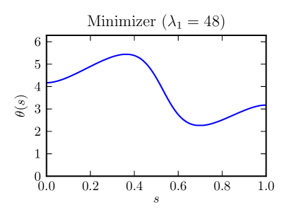
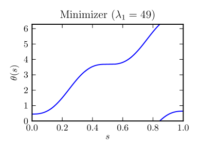
Figure 1: The minimizer $\theta(s)$ for the distance between a line and a circle at $\lambda_{1}=48$ and $\lambda_{1}=49$.

More general curves.

If we consider curves beyond these simple examples, then we quickly run into boundary value problems that do not have explicit solutions anymore. For example, comparing a straight line $c_{1}$ to a curve that is a graph, $c_{2}(s)=(s,h(s))$, we find that (16) reduces to

$$\theta^{\prime\prime}(s)=-\frac{\lambda_{1}}{2}\big{(}\sin(\theta(s))-\cos(\theta(s))h^{\prime}(s)\big{)}.$$

This is reminiscent of the pendulum equation (19), except that the magnitude and direction of gravity now explicitly depend on $s$ through $h^{\prime}(s)$. Although analytical solutions are out of reach here, these equations can easily be solved numerically (also in higher dimensions) and minimizers can be found by using adjoint equations to solve the boundary value problem with a Newton–Raphson method.

Equations in $\mathbb{R}^{3}$.

Finally, let us express the equations (13) in three dimensions, first with $k=1$. The identification of Lie algebra elements $\Omega\in\mathfrak{o}(n)$ and $\omega\in(\mathbb{R}^{3},\times)$ via $\Omega_{ij}=\epsilon_{ijk}\,\omega_{k}$ allows us to identify $\Omega=A\diamond B^{\flat}$ with

$$\omega_{k}=\frac{1}{2}\epsilon_{ijk}\Omega_{ij}=\frac{\lambda_{1}}{2}\epsilon_{ijk}A_{i}B_{j}.$$

Equation (13) then becomes

$$\omega^{\prime}(s)=\frac{\lambda_{1}}{2}\big{(}g(s)^{-1}\cdot c_{2}^{\prime}(s)\times c_{1}^{\prime}(s)\big{)}$$ (20)

where $g(s)\in O(3)$ and $\times$ now denotes the usual cross product on $\mathbb{R}^{3}$. Note that this generalizes to arbitrary $k$ as

$$\omega^{\prime}(s)=\frac{1}{2}\sum_{i=1}^{k}\lambda_{i}\big{(}g(s)^{-1}\cdot c_{2}^{(i)}(s)\times c_{1}^{(i)}(s)\big{)}.$$

6 The Existence of a Minimizer

We now prove that there exists a minimizer for the curve-matching functional. Our approach follows closely the proof of minimizers for the LDDMM functional in [BH13, You10], while also using some theory on Hilbert manifolds, see [Pal63, Kli95].

Let $O(n)$ be the orthogonal group in $n$ dimensions, with Lie algebra $\mathfrak{o}(n)$. In (4) we defined the inner product $\langle\xi,\eta\rangle_{\mathfrak{o}(n)}:=-\operatorname{tr}(\xi\eta)$. As this is a positive definite $\operatorname{Ad}$-invariant quadratic form, it determines a bi-invariant Riemannian metric on $O(n)$ with induced distance $d(\,\cdot\,,\,\cdot\,)_{O(n)}$. Therefore, $L^{2}(I,\mathfrak{o}(n))$ is a Hilbert space and $H^{1}(I,O(n))$ can be viewed as a $C^{\infty}$ Hilbert manifold [Kli95, Thm. 2.3.12] (see also [Pal63, §13, Thm. 6] but note that Palais’ definition of manifold structure is slightly different due to the use of an embedding).

We briefly recall Definition [Kli95, Def. 2.3.1] of the Hilbert manifold $H^{1}(I,M)$ where $M$ is a complete Riemannian manifold: it consists of the curves $c\in C^{0}(I,M)$ such that for any chart $(\phi,U)$ of $M$ and $I^{\prime}=c^{-1}(U)$ we have $\phi\circ c\in H^{1}(I^{\prime},\mathbb{R}^{n})$. Canonical charts for $H^{1}(I,M)$ are given by the exponential map along piecewise smooth curves $c$.

This Hilbert manifold comes equipped with a natural inner product which turns it into an infinite-dimensional Riemannian manifold. Let $c\in H^{1}(I,M)$ and let $\lambda,\mu\in H^{1}(c^{*}(\mathrm{T}M))$ denote sections in the pullback bundle, i.e. $\lambda(s),\mu(s)\in\mathrm{T}_{c(s)}M$ for all $s\in I$. This pullback bundle serves as a natural chart for the tangent space $\mathrm{T}_{c}H^{1}(I,M)$. The Riemannian metric on $H^{1}(I,M)$ is given in this chart by

$$\langle\lambda,\mu\rangle_{H^{1}(I,M)}=\int_{I}\Big{(}\langle\lambda(s),\mu(s)\rangle_{M}+\langle\nabla\lambda(s),\nabla\mu(s)\rangle_{M}\Big{)}{\;\textrm{d}}s,$$ (21)

where $\nabla$ denotes the covariant derivative pulled back from $\mathrm{T}M$ to $c^{*}(\mathrm{T}M)$.

Having this preliminary theory at hand, we can now state the following result in the case that $M=O(n)$.

Theorem 6.1.

The energy functional $E\colon H^{1}(I,O(n))\to\mathbb{R}$ defined by (7) attains its global minimum on $H^{1}(I,O(n))$. Moreover, any minimizer $g^{*}\in H^{1}(I,O(n))$ satisfies the variational equations (13) and in particular $g^{*}\in C^{2}(I,O(n))$.

We first identify the space $H^{1}(I,O(n))$ with a simpler one. This identification we can make in general, for any Lie group $G$ equipped with a left (or right) invariant inner product, such that $G$ is a Riemannian manifold.

Proposition 6.2.

Let $G$ be a Lie group equipped with a left-invariant inner product and let $\mathfrak{g}$ denote its Lie algebra. There is a natural bijection $\phi\colon H^{1}(I,G)\to G\times L^{2}(I,\mathfrak{g})$ given by

$$\phi(g)=(g(0),s\mapsto g(s)^{-1}g^{\prime}(s)),$$ (22)

and $g=\phi^{-1}(g_{0},\xi)$ is given by the reconstruction equation

$$g^{\prime}(s)=g(s)\xi(s)\quad\text{with initial conditions }g(0)=g_{0}.$$ (23)

Proof.

For $g\in H^{1}(I,G)$ it follows that $s\mapsto\xi(s)=g(s)^{-1}g^{\prime}(s)\in L^{2}(I,\mathfrak{g})$ since $g^{\prime}\in L^{2}(I,\mathrm{T}O(n))$ by definition, and left-translation by $g(s)^{-1}$ is a linear isomorphism and continuous (thus bounded) in $s$, hence it is a bounded operator on $L^{2}(I,\mathrm{T}G)$ that maps $g(s)^{-1}g^{\prime}(s)\in\mathrm{T}_{e}G=\mathfrak{g}$. Clearly, also $g(0)\in G$. Hence, $\phi$ is well-defined.

To prove that $\phi$ is a bijection, we show that $\phi^{-1}$ is well-defined and indeed the inverse of $\phi$. Viewing $\xi(s)$ as a left-invariant vector field on $G$ turns (23) into a Carathéodory type differential equation on $G$, since $\xi\in L^{2}(I,\mathcal{X}(G))$ with respect to local charts $(\psi,U)$ on $G$. By left-invariance of the metric on $G$ it follows that the left-invariant vector field $\xi$ is bounded by an integrable function:

$$\int_{I}\sup_{g\in G}\lVert\xi(s,g)\rVert{\;\textrm{d}}s=\int_{I}\lVert\xi(s)\rVert{\;\textrm{d}}s=\lVert\xi\rVert_{L^{1}(I,\mathfrak{g})}\leq\lVert\xi\rVert_{L^{2}(I,\mathfrak{g})}<\infty.$$

Theorem 2.1 in [CL55, Chap. 2] then implies local existence and uniqueness of the solution of (23) with respect to a chart $(\psi,U)$. By Theorem 1.3 in [CL55, Chap. 2] these solutions extend to the boundary of $\psi(U)$, hence they can be patched together to a maximal solution $g\colon I\to G$. Solution curves are by construction $H^{1}$ functions with respect to these charts and in view of the definition of $H^{1}(I,G)$, this implies that $\phi^{-1}$ is well-defined. Existence and uniqueness now implies that $\phi^{-1}$ is the inverse of $\phi$. ∎

Lemma 6.3.

Let $C^{0}(I,O(n))$ be equipped with the supremum distance

$$d(g,h)_{\sup}=\sup_{s\in I}\;d(g(s),h(s))_{O(n)}.$$ (24)

The map $\phi^{-1}$ is continuous into $C^{0}(I,O(n))$; moreover it maps bounded, weakly convergent sequences onto convergent sequences.

We summarize Theorems 8.7 and 8.11 from [You10] below, and use this result as the basic ingredient for the proof of the lemma.

Theorem 6.4.

Let $v^{*}\in L^{1}(I,C_{0}^{1}(\Omega,\mathbb{R}^{d}))$ be a time-dependent vector field with support in the open, bounded set $\Omega\subset\mathbb{R}^{d}$, and let $v_{i}\in L^{1}(I,C_{0}^{1}(\Omega,\mathbb{R}^{d}))$ be a bounded sequence, weakly convergent to $v^{*}$. Then the respective flows $\phi^{*},\phi_{i}$ are diffeomorphisms at all times, and $\phi_{i}\to\phi^{*}$ in supremum norm on $\bar{\Omega}$.

Proof of Lemma 6.3.

Note that it is sufficient to prove the last, stronger claim. Let $\xi\in L^{2}(I,\mathfrak{o}(n))$ and $g_{0}\in O(n)$, and let $g=\phi^{-1}(g_{0},\xi)$. In order to apply Theorem 6.4, we shall embed everything in linear spaces. Note that $O(n)$ has the usual isometric embedding into the space of matrices, $M_{n}\cong\mathbb{R}^{n\times n}$, and the Frobenius inner product corresponds to the normal Euclidean one. We interpret elements $\eta\in\mathfrak{o}(n)$ as left-invariant vector fields on $O(n)$. These can be smoothly extended to have compact support on an $O(n)$-invariant tubular neighborhood of $O(n)\subset M_{n}$. Thus, $\xi\in L^{2}(I,\mathfrak{o}(n))$ defines a time-dependent vector field on $M_{n}$ with compact support, that is smooth with respect to $g\in M_{n}$ and square-integrable with respect to $s\in I$. Since $I$ is bounded, this implies absolute integrability, satisfying the conditions of Theorem 6.4. The extended vector field leaves $O(n)$ invariant and is identical to the original $\eta$ on $O(n)$, so the generated flow can be restricted to a flow on $O(n)$, which is the one generated by $\eta$.

Next, we claim that there exists a $C\geq 1$ such that

$$C^{-1}d(g,g^{\prime})_{O(n)}\leq\lVert g-g^{\prime}\rVert_{M_{n}}\leq Cd(g,g^{\prime})_{O(n)}.$$ (25)

Note that the second inequality follows straightforwardly (with $C=1$) from the isometric embedding $O(n)\subset M_{n}$. We sketch the argument for the first inequality, more details can be found in [Eld13, Lem. 2.25]. Using symmetry, we need only prove the case where $g^{\prime}=e$. For a sufficiently small $\delta>0$ and $d(e,g)_{O(n)}<\delta$, we can consider $B(e;\delta)\subset O(n)$ and view it as the graph of the function $\exp\colon\mathfrak{o}(n)\to M_{n}$ which has identity derivative at $e$, thus we can bound $\lVert\mathrm{D}\exp-I\rVert\leq\frac{1}{2}$, say, on $B(e;\delta)$. Now we write

$$g-e=\int_{0}^{1}\mathrm{D}\exp(t\log(g))\cdot\log(g){\;\textrm{d}}t,$$

from which the estimate

$$\lVert g-e\rVert_{M_{n}}\geq\int_{0}^{1}\frac{1}{2}\lVert\log(g)\rVert{\;\textrm{d}}t=\frac{1}{2}d(e,g)_{O(n)},$$

follows. For $d(e,g)_{O(n)}>\delta$ we can simply choose $C\geq\text{diam}_{M_{n}}(O(n))/\delta$.

Finally, we note that $L^{2}(I,M_{n})$ is continuously embedded into $L^{1}(I,M_{n})$ and apply Theorem 6.4 to conclude that $\phi^{-1}$ maps bounded, weakly convergent sequences into convergent sequences in $C^{0}(I,O(n)_{M_{n}})$, where $O(n)_{M_{n}}$ denotes $O(n)$ with the distance induced by the embedding into $M_{n}$. By (25) this distance is equivalent to the intrinsic distance on $O(n)$, hence the result follows. ∎

The registration functional.

We will prove the existence of a minimizer for a slightly more general functional, given by

$$E(g)=V(g)+T(g)=\int_{I}\Big{(}U(s,g(s))+\frac{1}{2}\lVert\xi(s)\rVert^{2}\Big{)}{\;\textrm{d}}s,$$ (26)

where $\xi(s)=g(s)^{-1}g^{\prime}(s)\in\mathfrak{o}(n)$ and $V$ and $T$ denote the potential and kinetic parts of the functional, respectively. The function $U\colon I\times O(n)\to\mathbb{R}$ is assumed to be continuous, and the derivative with respect to the second variable, $\mathrm{D}_{2}U$, also continuous.

We take a minimizing sequence $g_{i}\in H^{1}(I,O(n))$, that is,

$$\lim_{i\to\infty}E(g_{i})=\inf_{g\in H^{1}(I,O(n))}E(g).$$

Since $\lim_{\lVert g\rVert_{H^{1}}\to\infty}E(g)=\infty$, it follows that this sequence is bounded. Using $\phi$ from Proposition 6.2 we can identify this sequence with a sequence $(g_{0},\xi)_{i}\in O(n)\times L^{2}(I,\mathfrak{o}(n))$.

In the following we take subsequences without denoting these with new indices. First, since $O(n)$ is compact, we can take a subsequence such that $(g_{0})_{i}$ converges to an element $g^{*}_{0}\in O(n)$. Secondly, since the sequence $\xi_{i}$ is bounded, we extract a subsequence such that $\xi_{i}$ converges weakly to some $\xi^{*}\in L^{2}(I,\mathfrak{o}(n))$. We show that $g^{*}=\phi^{-1}(g^{*}_{0},\xi^{*})$ is a minimizer of $E$.

We have automatically that

$$\inf_{g\in H^{1}(I,O(n))}E(g)\leq E(g^{*}),$$ (27)

and we now prove the reverse inequality. The only place in which our proof differs from the sketched proof of [BH13, Thm. 21] is in our treatment of the terms involving $U$. Let $g_{i}$ and $g^{*}$ be the solutions of the reconstruction equation (23) associated with $(g_{0},\xi)_{i}$ and $(g^{*}_{0},\xi^{*})$, respectively. By Lemma 6.3 we have that $g_{i}\to g^{*}$ under the supremum norm. The function $U$ is bounded since it is continuous on a compact domain; by the bounded convergence theorem we have therefore that

$$\lim_{i\to\infty}\int_{I}U(s,g_{i}(s)){\;\textrm{d}}s=\int_{I}U(s,g^{*}(s)){\;\textrm{d}}s,$$

that is, the functional defined by $U$ is continuous. The rest of the proof now proceeds as in [BH13]: from the inequality

$$\langle\xi_{i},\xi^{*}\rangle_{L^{2}}\leq\lVert\xi_{i}\rVert_{L^{2}}\lVert\xi^{*}\rVert_{L^{2}},$$

we have that $\lVert\xi^{*}\rVert_{L^{2}}\leq\liminf_{i\to\infty}\lVert\xi_{i}\rVert_{L^{2}}$, and therefore

$$E(g^{*}) =\frac{1}{2}\lVert\xi^{*}\rVert_{L^{2}}^{2}+\int_{I}U(s,g^{*}(s)){\;\textrm{d}}s$$

$$\leq\liminf_{i\to\infty}\frac{1}{2}\lVert\xi_{i}\rVert_{L^{2}}^{2}+\lim_{i\to\infty}\int_{I}U(s,g_{i}(s)){\;\textrm{d}}s$$

$$=\lim_{i\to\infty}E(g_{i})=\inf_{g\in H^{1}(I,O(n))}E(g).$$

This concludes the proof that the energy functional has a minimizer.

Finally, we can conclude that any minimizer of the energy functional is a solution of the variational equations (13) as follows. First, by Proposition 6.5 below $E$ is differentiable, hence at a minimizer $g\in H^{1}(I,O(n))$ we must have $\mathrm{D}E(g)=0$; this is equivalent to (12). The variational equations derived from this can be interpreted in a distributional sense, acting on variations $\delta\!g\in C^{\infty}(I,O(n))$. However, the equations (13) define a continuous vector field on $\mathrm{T}O(n)$ coming from a second order ODE, so solutions of it must be curves $g\in C^{2}(I,O(n))$, see for instance [Dui76, p. 178] or [BGH98, Thm. 4.1]. This completes the proof of Theorem 6.1.

Proposition 6.5.

The functional $E\colon H^{1}(I,O(n))\to\mathbb{R}$ given by (26) is differentiable.

Proof.

Differentiability of the kinetic term $T(g)$ follows from [Kli95, Thm. 2.3.20]. For the potential term $V(g)$, we claim that the derivative is given by

$$\mathrm{D}V(g)\delta\!g=\int_{I}\mathrm{D}_{2}U(s,g(s))\delta\!g(s){\;\textrm{d}}s.$$ (28)

Since $\mathrm{D}_{2}U$ is continuous on a compact domain, it is uniformly continuous; let $\epsilon$ denote its modulus of continuity. We directly estimate

$$\big{\lvert}V(g+\delta\!g)-V(g)-\mathrm{D}V(g)\delta\!g\big{\rvert}$$

$$=\int_{I}\big{\lvert}U(s,g(s)+\delta\!g(s))-U(s,g(s))-\mathrm{D}_{2}U(s,g(s))\delta\!g(s)\big{\rvert}{\;\textrm{d}}s$$

$$\leq\int_{I}\int_{0}^{1}\big{\lvert}\mathrm{D}_{2}U(s,g(s)+\tau\delta\!g(s))\delta\!g(s)-\mathrm{D}_{2}U(s,g(s))\delta\!g(s)\big{\rvert}{\;\textrm{d}}\tau{\;\textrm{d}}s$$

$$\leq\epsilon\big{(}\sup_{s\in I}\lVert\delta\!g(s)\rVert\big{)}\int_{I}\lVert\delta\!g(s)\rVert{\;\textrm{d}}s\in o(\lVert\delta\!g\rVert_{H^{1}}),$$

which proves our claim. ∎

7 Probabilistic approach to curve matching

The energy functional (7) can be derived from a Bayesian point of view as well. To see this, we adapt the Bayesian approach to linear regression (see for instance [Bis06]) to the case of curve matching. We first make the following simplifications:

1. We assume that the curves are planar and we let the order of the jets be $k=1$, so that only the tangent vector field of the curves is taken into account.

2. We only consider the tangent vector field at the end points of $N$ regularly spaced intervals in the parameter $s$. In other words, we sample $c_{1}^{\prime}(s)$ and $c_{2}^{\prime}(s)$ at $s_{n}=n\Delta s$ for $n=0,\ldots,N$, where $\Delta s=1/N$ and $n=0,\ldots N$. Later on, we will let $N$ approach infinity.

Throughout the remainder of this paragraph, we will use $\{c_{1}^{\prime}(s_{n})\}$ as a shorthand for the ensemble $\{c_{1}^{\prime}(s_{0}),\ldots,c_{1}^{\prime}(s_{N})\}$, and similarly for $\{c_{2}^{\prime}(s_{n})\}$.

Now let $c_{1}(s_{n})$ be fixed, and assume that, for each $n=0,\ldots,N$, $c_{2}^{\prime}(s_{n})$ is found by acting on $c_{1}^{\prime}(s_{n})$ with a rotation matrix $g_{n}$, and by adding noise:

$$c_{2}^{\prime}(s_{n})=g_{n}\cdot c_{1}^{\prime}(s_{n})+\epsilon_{n},$$

where the $\epsilon_{n}$ are $\mathbb{R}^{2}$-valued, independently distributed Gaussian random variables with mean $0$ and variance $\sigma^{2}/\lambda I$, where $I$ is the $2\times 2$ identity matrix. The constant $\lambda$ will play the same role as the scaling parameters in the norm (3).

The conditional probability to obtain the ensemble $\{c_{2}^{\prime}(s_{n})\}$ for $n=0,\ldots,N$, given $\{c_{1}^{\prime}(s_{n})\}$ and $\{g_{n}\}$ is

$$p(\{c_{2}^{\prime}(s_{n})\}\,|\,\{c_{1}^{\prime}(s_{n})\},\{g_{n}\})\propto\exp\left(-\frac{\lambda}{\sigma^{2}}\Delta s\sum_{n=0}^{N}\lVert c_{2}^{\prime}(s_{n})-g_{n}\cdot c_{1}^{\prime}(s_{n})\rVert^{2}\right).$$

Now assume that we choose a prior on the space of discrete curves $\{g_{n}\}$ which privileges curves which are nearly constant. For instance, we may choose

$$p(\{g_{n}\})\propto\exp\left(-\frac{1}{\Delta s}\sum_{n=0}^{N-1}\lVert g_{n+1}-g_{n}\rVert^{2}\right),$$

where $\lVert\,\cdot\,\rVert$ is the Frobenius norm on the space of matrices. By Bayes’ theorem, we can then calculate the conditional probability for $\{g_{n}\}$ given $\{c_{1}^{\prime}(s_{n})\}$ and $\{c_{2}^{\prime}(s_{n})\}$ as

$$p(\{g_{n}\}\,|\,\{c_{1}^{\prime}(s_{n})\},\{c_{2}^{\prime}(s_{n})\})\propto p(\{c_{2}^{\prime}(s_{n})\}\,|\,\{c_{1}^{\prime}(s_{n})\},\{g_{n}\})p(\{g_{n}\}),$$

where we have used the fact that $g_{n}$ is independent from $c_{1}^{\prime}(s_{n})$, so that $p(\{g_{n}\}|\{c_{1}^{\prime}(s_{n})\})=p(\{g_{n}\})$. The negative logarithm of this density is given by

$$-\log p(\{g_{n}\}\,|\,\{c_{1}^{\prime}(s_{n})\},\{c_{2}^{\prime}(s_{n})\})=\\ \frac{\lambda}{\sigma^{2}}\Delta s\sum_{n=0}^{N}\lVert c_{2}^{\prime}(s_{n})-g_{n}\cdot c_{1}^{\prime}(s_{n})\rVert^{2}+\frac{1}{\Delta s}\sum_{n=0}^{N-1}\lVert g_{n+1}-g_{n}\rVert^{2},$$ (29)

and for $N\to\infty$, this gives precisely the matching energy (7). From this point of the view, the curve $g(s)$ that minimizes (7) is precisely the maximum posterior estimate of (the continuum version of) the distribution (29).

8 Conclusions and outlook

In this paper, we have defined a notion of distance between parametrized curves in $\mathbb{R}^{n}$, and we have shown (among other things) that — in contrast to previous approaches — this notion is a true distance function. Our approach uses only standard geometrical notions, and is hence eminently generalizable. Below, we describe some directions for future research.

Statistical analysis of curves and shapes.

Using the distance function on the space of curves defined in this paper (and its generalization to surfaces, described below), we can embark on a statistical analysis of shapes and curves. Having a notion of distance will allow us to register curves, compute (Fréchet) means, and use tools from Riemannian geometry in the exploration of shape geometries; see [Pen06] for more details.

Matching of surfaces.

The method presented in this paper naturally generalizes to matching of parametrized (2D) surfaces in $\mathbb{R}^{n}$. We sketch here the setup; for simplicity of presentation we set $k=1$ and take as parametrization domain the torus $\mathbb{T}^{2}=[0,1]^{2}/\sim$, where $\sim$ identifies opposite edges of the unit square. Then the energy functional becomes

$$E[g;f_{1},f_{2}]=\frac{1}{2}\int_{[0,1]^{2}}\lVert g(s,t)\cdot\mathrm{D}f_{1}(s,t)-\mathrm{D}f_{2}(s,t)\rVert^{2}+\lVert g(s,t)^{-1}\mathrm{D}g(s,t)\rVert^{2}{\;\textrm{d}}s{\;\textrm{d}}t,$$ (30)

with $g\colon\mathbb{T}^{2}\to O(n)$ and $f_{i}\colon\mathbb{T}^{2}\to\mathbb{R}^{n}$, $\mathrm{D}$ denotes a derivative with respect to both variables $s,t$ and the norms are now defined on pairs of elements in $V$ and $\mathfrak{o}(n)$ respectively, by a square-root of the sum of squares. Finally, $g(s,t)$ simply acts on each element of the pairs. The variation of the functional, $\delta\!E$, now contains a derivative both with respect to $s$ and $t$. Integrating each by parts, this leads to the variational equations

$$\mathrm{D}_{s}\Omega_{s}+\mathrm{D}_{t}\Omega_{t}=(g^{-1}\cdot\mathrm{D}f_{2})\diamond(\mathrm{D}f_{1})^{\flat},$$ (31)

where everything depends on $(s,t)$ and the subscript $s,t$ denote derivatives and components with respect to these. This equation naturally generalizes (13), although it is now a second order partial differential equation. To decompose this into first order PDEs, one has to add the equation

$$\mathrm{D}_{s}\Omega_{t}-\mathrm{D}_{t}\Omega_{s}=\big{[}\Omega_{t}\,,\,\Omega_{s}\big{]}$$ (32)

that expresses symmetry of the second order derivatives of the underlying $g(s,t)$. This formulation is closely related to that of a $G$-strand and (32) is known as the zero curvature relation, see [HIP12].

Generalizations to curved manifolds.

From a geometric point of view, it would be interesting to consider the extension of this framework to the case of curves taking values in an arbitrary Riemannian manifold $M$. One immediate difficulty is that the matching term in (7) involves the difference of jets at different points. To remedy this, one could either choose a flat background connection, if possible, and parallel translate the jets to a common base point. Another possibility would be to replace the group $O(n)$ by the orthogonal groupoid $O(\mathrm{T}M,\mathrm{T}M)$, consisting of linear bundle isometries from $\mathrm{T}M$ to $\mathrm{T}M$. If we view the combined source and target maps $(\alpha,\beta)\colon O(\mathrm{T}M,\mathrm{T}M)\to M\times M$ as a projection defining a fiber bundle, then $g\in H^{1}(I,O(n))$ is generalized to being a section

$$g\in H^{1}\big{(}(c_{1},c_{2})^{*}O(\mathrm{T}M,\mathrm{T}M)\big{)},$$

that is, we have $g(s)\in O(\mathrm{T}_{c_{1}(s)}M,\mathrm{T}_{c_{2}(s)}M)$. The action of $g(s)$ on a jet $j^{k}_{s}c_{1}$ can be defined by its action on the covariant derivatives of $c_{1}$. Parallel transported orthonormal frames along the curves $c_{i}$ will allow representing $g^{\prime}(s)$ in $\mathfrak{o}(n)$.

References

- [AM78] Ralph Abraham and Jerrold E. Marsden “Foundations of mechanics” Second edition, revised and enlarged, With the assistance of Tudor Raţiu and Richard Cushman Reading, Mass.: Benjamin/Cummings Publishing Co. Inc. Advanced Book Program, 1978, pp. xxii+m–xvi+806 URL: http://www.cds.caltech.edu/~marsden/books/Foundations_of_Mechanics.html
- [Bis06] Christopher M. Bishop “Pattern recognition and machine learning”, Information Science and Statistics New York: Springer, 2006, pp. xx+738 DOI: 10.1007/978-0-387-45528-0
- [BH13] Martins Bruveris and Darryl D. Holm “Geometry of Image Registration: The Diffeomorphism Group and Momentum Maps” To appear in the Fields Institute Communications series volume “Geometry, Mechanics, and Dynamics: The Legacy of Jerry Marsden”, 2013 arXiv:1306.6854 [math.DG]
- [BGH98] Giuseppe Buttazzo, Mariano Giaquinta and Stefan Hildebrandt “One-dimensional variational problems” An introduction 15, Oxford Lecture Series in Mathematics and its Applications The Clarendon Press, Oxford University Press, New York, 1998, pp. viii+262
- [CM87] Hernan Cendra and Jerrold E. Marsden “Lin constraints, Clebsch potentials and variational principles” In Phys. D 27.1-2, 1987, pp. 63–89 DOI: 10.1016/0167-2789(87)90005-4
- [CL55] Earl A. Coddington and Norman Levinson “Theory of ordinary differential equations” McGraw-Hill Book Company, Inc., New York-Toronto-London, 1955, pp. xii+429
- [Dui76] J. J. Duistermaat “On the Morse index in variational calculus” In Advances in Math. 21.2, 1976, pp. 173–195 DOI: 10.1016/0001-8708(76)90074-8
- [Eld13] Jaap Eldering “Normally hyperbolic invariant manifolds — The noncompact case” 2, Atlantis Series in Dynamical Systems Paris: Atlantis Press, 2013, pp. xii+189 DOI: 10.2991/978-94-6239-003-4
- [HNV13] D. D. Holm, L. Noakes and J. Vankerschaver “Relative geodesics in the special Euclidean group” In Proc. R. Soc. Lond. Ser. A Math. Phys. Eng. Sci. 469.2158, 2013, pp. 1471–2946 DOI: 10.1098/rspa.2013.0297
- [HIP12] Darryl D. Holm, Rossen I. Ivanov and James R. Percival “-Strands” In J. Nonlinear Sci. 22.4, 2012, pp. 517–551 DOI: 10.1007/s00332-012-9135-4
- [Kli95] Wilhelm P. A. Klingenberg “Riemannian geometry” 1, de Gruyter Studies in Mathematics Berlin: Walter de Gruyter & Co., 1995, pp. x+409 DOI: 10.1515/9783110905120
- [MR94] Jerrold E. Marsden and Tudor S. Ratiu “Introduction to mechanics and symmetry” 17, Texts in Applied Mathematics New York: Springer-Verlag, 1994
- [Pal63] Richard S. Palais “Morse theory on Hilbert manifolds” In Topology 2, 1963, pp. 299–340 DOI: 10.1016/0040-9383(63)90013-2
- [Pen06] Xavier Pennec “Intrinsic Statistics on Riemannian Manifolds: Basic Tools for Geometric Measurements” In Journal of Mathematical Imaging and Vision 25.1 Kluwer Academic Publishers, 2006, pp. 127–154 DOI: 10.1007/s10851-006-6228-4
- [You10] Laurent Younes “Shapes and diffeomorphisms” 171, Applied Mathematical Sciences Berlin: Springer-Verlag, 2010, pp. xviii+434 DOI: 10.1007/978-3-642-12055-8