Communication on structure of biological networks

Abstract

Networks are widely used to represent interaction pattern among the components in complex systems. Structures of real networks from different domains may vary quite significantly. Since there is an interplay between network architecture and dynamics, structure plays an important role in communication and information spreading on a network. Here we investigate the underlying undirected topology of different biological networks which support faster spreading of information and are better in communication. We analyze the good expansion property by using the spectral gap and communicability between nodes. Different epidemic models are also used to study the transmission of information in terms of disease spreading through individuals (nodes) in those networks. Moreover, we explore the structural conformation and properties which may be responsible for better communication. Among all biological networks studied here, the undirected structure of neuronal networks not only possesses the small-world property but the same is expressed remarkably to a higher degree than any randomly generated network which possesses the same degree sequence. A relatively high percentage of nodes, in neuronal networks, form a higher core in their structure. Our study shows that the underlying undirected topology in neuronal networks is significantly qualitatively different than the same from other biological networks and that they may have evolved in such a way that they inherit a (undirected) structure which is excellent and robust in communication.

1 Introduction

Over the past few years, network science has drawn attention from a large number of researchers from diverse fields. Networks in which the underlying topology is a graph, are generic representations of the interactions among components of a complex system. Biological networks provide an insight to analyze and understand various processes that occur in several biological systems. These systems range from intracellular protein interactions to inter-species interactions (see [22] for details). Most networks have the function to transport or transfer entities like information, mass, energy etc. along their edges. Structure of a network plays a crucial role in spreading of the above entities. In the last few years different heuristic parameters (clustering coefficient, transitivity, average path length, betweenness, centrality etc. see [21] for details) have been introduced for analyzing the network structure, and various models (e.g. Erdös-Rényi’s model random network model, Barabási and Albert’s scale free model, Watts and Stogatz’s small-world network model, duplication-divergence model etc. [10, 1, 27, 17]) have been proposed to represent the architecture of real networks. The qualitative properties of biological networks cannot be well captured by the heuristic parameters. However, spectral analysis is also used for elucidating the global property of a network (see [14, 15]). Features like “good expansion” and “communicability” are well quantified by spectral analysis (see [5, 6]). Good expansion network can be thought of as a network in which a small subset of vertices has comparatively large number of neighbours (see [9, 5, 6]) and communicability can be understood as networks in which information is “capable of being easily communicated or transmitted in terms of passage or means of passage between the different nodes in a network” (see [12]).

Here, we study the underlying undirected structure of empirical biological networks from five different classes (neuronal, food web, protein protein interaction, metabolism and gene regulation) and explore the undirected topology that supports better communication and information spreading. We observe that one class of biological networks has higher good expansion property and excellent communicability than the others, though most of the biological networks (see [27]) have high clustering coefficients (or transitivity) and low average shortest path lengths which give them the liberty to reach from one node to another with a fewer number of steps. This property of a network is quite well known as the small-world property (see [27]). Here, we have also investigated the topological properties that make a particular class of biological networks possess the excellent expansion property.

2 Methods

Spectral gap and Good expansion network:

Generally, sparsely populated and highly connected network topologies are contradictory properties and hard to find in real-world networks. However, good expansion networks are known to possess those properties. There are extensive applications of good expansion networks in designing algorithms, error correcting codes, extractors, pseudo-random generators ([29]) etc. Good expansion networks are also important as they show excellent communication properties ([13]). The excellent spreading property or the good expansion property can be captured by the spectral gap in a network (see [26, 2]).

A network can be represented as a simple graph $G=(V,E)$, where $|V|$ (=n) is the number of vertices or nodes and $|E|$ is the number of connections or edges between nodes. An unweighted and undirected network has the good expansion property, if any set $S\subset V$ with $|S|\leq|V|/2$ satisfies

$$|S^{{}^{\prime}}|\geq c|S|,$$

where $S^{{}^{\prime}}\subset V\setminus S$ is the set of neighbours of $S$ and $c$ is a parameter called the expander constant (see [13, 24]). The adjacency matrix $A$ = ($A_{ij}$) corresponding to a graph $G$ is an $n\times n$ matrix with entries in {0, 1} such that $A_{ij}$ = 1, if there exists an edge in $G$ between the vertices $i$ and $j$, and 0 otherwise. The set of eigenvalues $\lambda_{1}\geq\lambda_{2}\geq\dots\geq\lambda_{n}$ of $A$ is called the spectrum of the network. The larger the spectral gap $|\lambda_{1}|-|\lambda_{2}|$ is, the faster the random walk (on the graph) will converge to its steady-state. Observe that the largest eigenvalue is always positive. Thus, a network shows good information spreading character if the largest eigenvalue of $A$ is much higher than the absolute value of the second largest eigenvalue (see [26, 2]), i.e. if

$$|\lambda_{1}|\gg|\lambda_{2}|.$$

Communicability:

Spreading of information, mass or entities on a network is a common process and eventuates in most networks. The nature of information or entities varies depending on the type of network. In neuronal networks, information spreading means electrical signal propagation. In food webs, it is regarded as mass flow from prey to predator. In signal transduction networks, it is the signal which spreads, and so on. Earlier, from a structural perspective, it was considered that the communication (information, mass, entities spreading) between two nodes in a network can happen only through the shortest routes connecting them because it is the most economical way of communication. But, communication between two nodes in a real network may not always only happen via the shortest routes.

Communicability can be thought of as transforming information easily between different nodes in a network. Communicability in a complex network is a broad generalization of the concept of the shortest path. To study the communicability, the above situations should be taken under consideration. Hence, communicability can be thought as how effectively information can be propagated between a pair of nodes in a network. We consider the communicability, introduced in [12], to study which undirected (biological) network structures are more favourable for excellent communication.

The $(i,j)$-entry of the $k^{th}$ power of the adjacency matrix $A^{k}$ shows the number of walks of length $k$ between the vertices $i$ and $j$. The information in a network can flow back and forth several times before reaching the final destination, like particle transversal through the graph. The communicability between any two nodes $p,q$ of a graph $G$ is defined by

$$G_{pq}=\sum_{j=1}^{n}\phi_{j}(p)\phi_{j}(q)e^{\lambda_{j}},$$ (2.0.1)

where $\phi_{j}(p)$ is the $p^{th}$ element of the $j^{th}$ orthonormal eigenvector corresponding to the eigenvalue $\lambda_{j}$. A large $G_{pq}$ implies that the communicability between the nodes $p$ and $q$ is high (see [12] for details).

Epidemic spreading in network:

Different epidemic models can be used to describe transmission of information in terms of disease spreading through individuals (nodes) in a network. Here, we study the nature of information spreading in the empirical networks by using three epidemic models, the SI (susceptible-infected) model, the SIR (susceptible-infected-recovered) model, and the SIS (susceptible-infected-susceptible) model (see  [21] for details on these models). We use these models for characterising the underlying undirected structures of biological networks which are more favourable in spreading information or disease.

The SI model: The simplest mathematical model among all epidemic models is the SI model consisting of two states, the susceptible and the infected individual. An individual who does not have the disease yet, but can catch the disease from infected individuals if in contact with them, is treated as susceptible. Infected individuals are those who currently have the disease and can infect susceptible individuals (see  [21]).

Suppose that a disease is spreading in a population of $n$ individuals. Let $s(t)$ and $x(t)$ denote the fraction of susceptible and infected individuals respectively at time t. If one infected individual can infect $\beta$ number of susceptible individuals per unit time, then the differential equations for the rate of change of x and s become

$$\left.\begin{aligned} \frac{dx}{dt}&=\beta{sx},\\ \frac{ds}{dt}&=-\beta{sx}.\end{aligned}\right\}$$ (2.0.2)

We randomly choose a node as infected and an infected node can infect its neighbours with infection probability 1.

The SIR model: The SIR model unlike the SI model, consists of three states, namely, susceptible, infected and recovered. Susceptible individuals are infected by the infected ones and the infected individuals are immunised. Immunised individuals are entered into the recovered state. Initially every individual is in the susceptible state except a small number of individuals. At each time step, one individual can infect their neighbour. Infected individuals are entered into the recovered state by immunisation.

If $s(t)$, $x(t)$, and $r(t)$ denotes the fraction of susceptible, infected and recovered individuals respectively at time $t$, then the equations for the SIR model are

$$\left.\begin{aligned} \frac{ds}{dt}&=-\beta{sx},\\ \frac{dx}{dt}&=\beta{sx}-\gamma{x},\\ \frac{dr}{dt}&=\beta{x},\end{aligned}\right\}$$ (2.0.3)

where $s+x+r=1$.

The SIS model: Here, the individuals can have two states susceptible and infected, like in the SI model. The only difference is that infected individuals after recovery, can become susceptible again.

The governing equations for this model are

$$\left.\begin{aligned} \frac{ds}{dt}&=\gamma{x}-\beta{sx},\\ \frac{dx}{dt}&=\beta{sx}-\gamma{x},\end{aligned}\right\}$$ (2.0.4)

with the condition $s+x=1$.

3 Network construction and Data resources:

Neuronal network: The data for macaque visual cortex, macaque visual and sensorimotor area, macaque cortical connectivity, cat cortex (complete), and cat cortex connectivity that was used by Rubinov and Sporns in [23] was downloaded from https://sites.google.com/site/bctnet/Home. To construct a network from these data, we consider the cortical areas as nodes and large corticocortical tracts as edges of the network. Neuronal connectivity data of C. elegans which was used by Watts and Strogatz in ([27]) and by White et al. in ([28]) was downloaded from http://www-personal.umich.edu/~mejn/netdata/. The nodes and edges of the network represent the neurons and the synaptic connections respectively.

Food web: Here, different species in the ecosystem are considered as nodes and the prey-predator relationships are considered as the edges of the network. The data was downloaded from http://www.cosinproject.org/.

Protein-protein interaction network: Here the nodes are proteins and we connect two proteins by an edge if they physically bind together. The E. coli data which was also used by Butland in ([7]), was downloaded from http://www.cosinproject.org.

Metabolic network: Here metabolites are represented by nodes and an educt-product relation is represented by an edge. The data was downloaded from http://www3.nd.edu/~networks/resources.htm (used in [18]).

Gene regulatory network: In this network, nodes are genes and if one gene regulates another we connect them by an edge. The data of E. coli and S. cerevisiae were downloaded from http://www.weizmann.ac.il/mcb/UriAlon/ (used in [20]).

4 Results and Discussion

Here, we study the underlying undirected structure of five different classes of biological networks: neuronal networks, food webs, protein-protein interaction networks, metabolic networks, gene regulatory networks. To investigate which structure is better for communication or spreading of mass, information or entities, we explore the good expansion property (by using the spectral gap) of a network and study the communicability between every pair of nodes. Different epidemic spreading models are also used to investigate the same on these networks.

We observe that the underlying undirected topology of all neuronal networks and a few food webs show the good expansion property (see Table 1) unlike other biological networks.

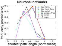
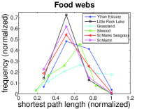
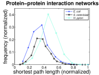
(a)                                         (b)                                        (c)

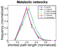
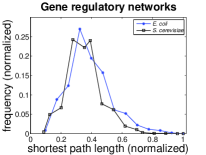
(d)                                         (e)

Figure 1: Histogram of shortest path length. X-axis represents the (normalized) shortest path length and Y-axis represents the (normalized) frequency. (a) Neuronal networks: (macaque visual cortex area, macaque large-scale visual and sensorimotor area corticocortical connectivity, macaque cortical connectivity, cat cortical area, cat cortical and thalamic areas, C. elegans), (b) Food webs: (Ythan Estuary, Little Rock Lake, Grassland, Silwood, St Marks Seagrass, St Martin), (c) Protein-protein interaction networks: (E. coli, S. cerevisiae, H. pylori), (d) Metabolic networks: archaea (A. pernix, A. fulgidus), eukaryota (E. nidulans, S. cerevisiae), bacteria (C. pneumoniae, N. gonorrhoeae), (g) Gene regulatory networks: (E. coli, S. cerevisiae).

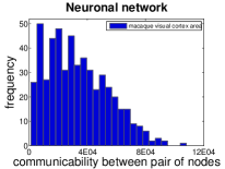
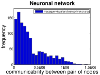
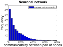
(a)                                      (b)                                   (c)

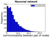
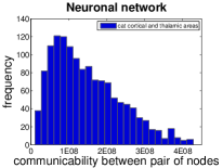
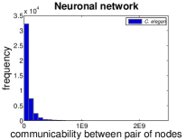
(d)                                      (e)                                   (f)

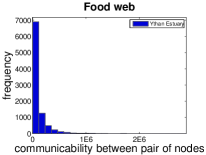
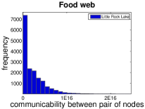
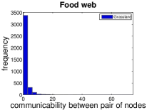
(g)                                      (h)                                   (i)

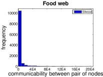
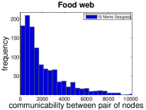
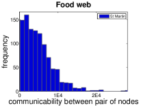
(j)                                      (k)                                       (l)

Figure 2: Histogram of communicability. Here the figures are the histogram of communicability (see equ 2.0.1) of neuronal networks and food webs. X-axis represent communicability between pair of nodes in a network and Y-axis represents frequency. Neuronal networks: (a) macaque visual cortex area, (b) macaque large-scale visual and sensorimotor area corticocortical connectivity, (c) macaque cortical connectivity, (d) cat cortical area, (e) cat cortical and thalamic areas, (f) C. elegans. Food webs: (g) Ythan Estuary, (h) Little Rock Lake, (i) Grassland, (j) Silwood, (k) St Marks Seagrass, (l) St Martin.

The distribution of the distances between every pair of nodes of each network (see Figure 1) follows a Gaussian like pattern, whereas, the distributions for the communicabilities for the same are different (see Figure 2, 3). They clearly show that the data (i.e., communicability between pairs of nodes) are positively skewed for most of the networks and the relative frequency is highly concentrated in a small interval of whole range, i.e. the relative frequencies for almost every interval is near zero except for a few intervals. Thus most networks have a small number of pairs of nodes that show high communicability. Remarkably the distribution pattern for the most of the neuronal networks and a few food webs are positively skewed and the data are spread out over the whole range in the sense that the relative frequency of almost each interval is significant (Figure 2). It reflects that the underlying undirected structure of most of the neuronal networks and a few food webs show high communicability between a relatively higher number of pairs of nodes within the network.

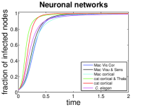
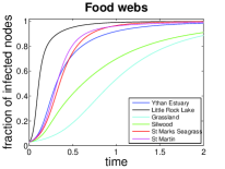
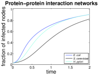
(a)                                             (b)                                   (c)

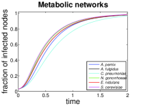
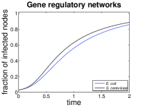
(d)                                         (e)

Figure 4: Dynamics of epidemics in SI model. X-axis represents time and Y-axis represents fraction of infected nodes in a network. (a) Neuronal networks: (macaque visual cortex area, macaque large-scale visual and sensorimotor area corticocortical connectivity, macaque cortical connectivity, cat cortical area, cat cortical and thalamic areas, C. elegans), (b) Food webs: (Ythan Estuary, Little Rock Lake, Grassland, Silwood, St Marks Seagrass, St Martin), (c) Protein-protein interaction networks: (E. coli, S. cerevisiae, H. pylori), (d) Metabolic networks: archaea (A. pernix, A. fulgidus), eukaryota (E. nidulans, S. cerevisiae), bacteria (C. pneumoniae, N. gonorrhoeae), (g) Gene regulatory networks: (E. coli, S. cerevisiae).

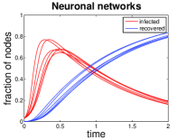
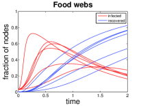
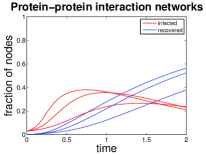
(a)                                         (b)                                        (c)

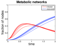
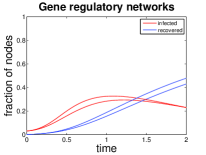
(d)                                         (e)

Figure 5: Dynamics of epidemics in SIR model. X-axis represents time and Y-axis represents fraction of nodes that are infected by red line and recovered by blue line. (a) Neuronal networks: (macaque visual cortex area, macaque large-scale visual and sensorimotor area corticocortical connectivity, macaque cortical connectivity, cat cortical area, cat cortical and thalamic areas, C. elegans), (b) Food webs: (Ythan Estuary, Little Rock Lake, Grassland, Silwood, St Marks Seagrass, St Martin), (c) Protein-protein interaction networks: (E. coli, S. cerevisiae, H. pylori), (d) Metabolic networks: archaea (A. pernix, A. fulgidus), eukaryota (E. nidulans, S. cerevisiae), bacteria (C. pneumoniae, N. gonorrhoeae), (g) Gene regulatory networks: (E. coli, S. cerevisiae).

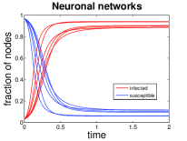
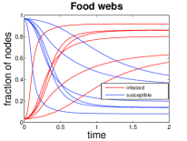
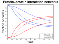
(a)                                               (b)                      (c)

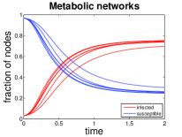
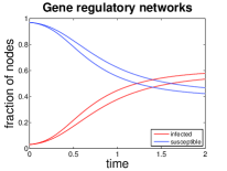
(d)                                   (e)

Figure 6: Dynamics of epidemics in SIS model. X-axis represents time and Y-axis represents fraction of nodes that are infected by red line and susceptible by blue line. (a) Neuronal networks: (macaque visual cortex area, macaque large-scale visual and sensorimotor area corticocortical connectivity, macaque cortical connectivity, cat cortical area, cat cortical and thalamic areas, C. elegans), (b) Food webs: (Ythan Estuary, Little Rock Lake, Grassland, Silwood, St Marks Seagrass, St Martin), (c) Protein-protein interaction networks: (E. coli, S. cerevisiae, H. pylori), (d) Metabolic networks: archaea (A. pernix, A. fulgidus), eukaryota (E. nidulans, S. cerevisiae), bacteria (C. pneumoniae, N. gonorrhoeae), (g) Gene regulatory networks: (E. coli, S. cerevisiae).

While studying the three epidemic models, we observe that in the SI model, the infection spreads faster on the underlying undirected structure of all neuronal networks than that of the other biological networks (see Figure 4). In the SIR model, the results show that the entire underlying undirected structure of all neuronal networks get infected, and also recover more rapidly compared to that of the other biological networks (see Figure 5). Similar results also hold in the SIS model for neuronal networks compared to the rest of the biological networks. In neuronal networks, states change quickly from susceptible to infected, and back again to susceptible, compared to the other biological networks studied here (see Figure 6).

Structural basis of information transfer:

We see that the underlying undirected structure of neuronal networks show high communicability and possess a good information spreading characteristic which is derived from the spectral gap. An epidemic can also spread faster on neuronal networks than the other biological networks studied here. Thus the underlying undirected architecture of a neuronal network possesses certain conformation which is favourable for spreading of different entities or information.

Now, to explore what are the topological characteristics that make the underlying undirected structure of a neuronal network very supportive for faster spreading of information, we investigate the small-world property and the small-world-ness of all the networks. We also study the same by randomizing the network, while conserving the degree sequence, to understand how small-world-ness relatively varies across a family of networks with the same degree sequence as in the given (undirected) network structure. To further investigate the architecture across various biological networks, we decompose the underlying undirected structure of a network into cores or shells.

The small-world property and small-world-ness:

In a small-world network, two nodes may not be directly connected, but, one can be reached from the other by a finite number of steps. Usually we see that small-world networks have a low average shortest path length and a high clustering coefficient (or transitivity) ([27]). A measure is defined on small-world property, called small-world-ness [16], as

$$SW_{G}=\frac{T_{G}/L_{G}}{T_{ER}/L_{ER}},$$

where $T_{G},L_{G}$ are the transitivity and average shortest path length of the network $G$ respectively. $T_{ER}$, $L_{ER}$ denote the same quantities for an Erdös-Rényi’s random graph with the same number of vertices and edges as $G$ (see [10, 11]). It is considered that the network $G$ has the small-world property if,

$$SW_{G}>1$$

.

Obviously, if a network $G$ has the small-world property, the ratio ($T_{G}/L_{G}$) is strictly higher than ($T_{ER}/L_{ER}$).

The underlying undirected structure of all the biological networks, studied here, have the small-world property. Now, we perform a relative study between small-world-ness of a network $G$ with its family $F_{G}$ for measuring the quality of the small-world property in $G$. A family $F_{G}$ of a network $G$, is a group of randomly generated networks which not only have the same number of vertices and edges but also have the same degree sequence as that of $G$. We see that not only the underlying undirected structure of all biological networks have the small-world property, but also, the families of all those networks possess the same property. For a qualitative study we define the z-score of small-world-ness of a network $G$ as

$$Z_{G}=\frac{SW_{G}-<SW_{F_{G}}>}{std(SW_{F_{G}})},$$

where $SW_{G}$ is the small-world-ness of the network $G$, $<SW_{F_{G}}>$ is the mean of small-world-ness of the family $F_{G}$ and $std(SW_{F_{G}})$ is the standard deviation of the family $F_{G}$.

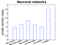
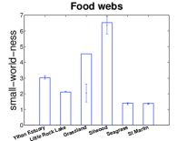
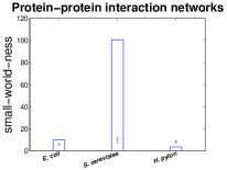
(a)                                         (b)                                        (c)

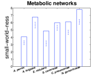
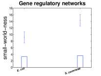
(d)                                         (e)

Figure 7: Histogram of small-world-ness of all biological networks. Here, a bin represents the small-world-ness of a network $G$ and errorbar represents the variability of small-world-ness of the family $F_{G}$ of $G$. $F_{G}$ is a set of networks have the same number of nodes and degree sequence as $G$ has. X-axis represents different networks of same class and y-axis represents small-world-ness of the corresponding networks. (a) Neuronal networks: (macaque visual cortex area, macaque large-scale visual and sensorimotor area corticocortical connectivity, macaque cortical connectivity, cat cortical area, cat cortical and thalamic areas, C. elegans), (b) Food webs: (Ythan Estuary, Little Rock Lake, Grassland, Silwood, St Marks Seagrass, St Martin), (c) Protein-protein interaction networks: (E. coli, S. cerevisiae, H. pylori), (d) Metabolic networks: archaea (A. pernix, A. fulgidus), eukaryota (E. nidulans, S. cerevisiae), bacteria (C. pneumoniae, N. gonorrhoeae), (g) Gene regulatory networks: (E. coli, S. cerevisiae)

We observe that all the neuronal networks have a positive and very high z-score (see Table 2, Figure 7(a)). Four among six food webs (Grassland, Silwood, St Marks Seagrass and St Martin) have positive, but low, z-scores and the rest possess negative z-scores (see Table  2, Figure  7(b)). Among all protein-protein interaction networks, E. coli and S. cerevisiae have positive z-scores unlike H. Pylori, which has a negative z-score (see Figure 7(c)). We study metabolic networks from three different domains, namely Archaea, Bacteria and Eucaryota. All of them have positive, but not high z-scores (see Figure 7(d),(e), (f)). All the gene regulatory networks studied here, E. coli and S. cerevisiae , have negative z-scores (see Figure 7(g)).

These z-scores topologically signify that the small-world-ness of each neuronal (undirected) network is higher than that of its family of networks and also possesses a highly positive z-score. Two gene regulatory networks E. coli and S. cerevisiae and one protein-protein interaction network S. cerevisiae show varied characteristics, and their small-world-ness is drastically different from their family. So among all biological networks, studied here, the underlying undirected structure of a neuronal network has special conformation. Not only, it has the small-world property, but also, it is expressed remarkably to a higher degree than any randomly generated network with the same (undirected) degree sequence. Thus, we see that the (undirected) structure of a neuronal network is more suitable for communication and information transfer.

The results above do not vary much even if the same study is done by generating 100, 200, or 300 networks in a family. Here, we show all the results over 200 realizations.

k-core decomposition:

It was considered that the dynamics of spreading information is very fast on a network having high degree nodes. Later on, it was shown that the vertices, which spread information efficiently, are not those with high degree or high betweenness centrality, but those that belong to a high k-core in the network ([19]).

A k-core of a graph $G$ is a maximal induced subgraph such that the degree of any vertex in that subgraph is grater than or equal to k. Thus a k-core of a graph can be obtained by recursively removing all the vertices of degree less than $k$, until the degrees of all nodes become at least $k$. A vertex with high degree may not belong to a high core, e.g. the centre vertex in a star graph is not located in a k-core for $k>1$. A vertex or node is assigned a shell index or equivalently coreness $k$, if it belongs to a k-core but not a k+1-core. All the vertices with shell index $k$ form a $k$-shell $S_{k}$. ( for more details on k-core decomposition see [21]).

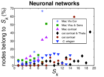
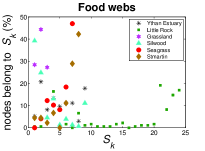
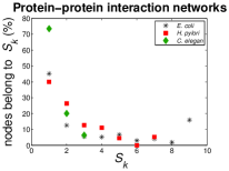
(a)                                         (b)                                        (c)

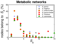
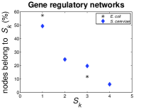
(d)                                       (e)

Figure 8: k-core decomposition of all biological networks. X-axis represents shell index k of k-shell $S_{\emph{k}}$ and Y-axis represents percentage of nodes belong to $S_{\emph{k}}$. (a) Neuronal networks: (macaque visual cortex area, macaque large-scale visual and sensorimotor area corticocortical connectivity, macaque cortical connectivity, cat cortical area, cat cortical and thalamic areas, C. elegans), (b) Food webs: (Ythan Estuary, Little Rock Lake, Grassland, Silwood, St Marks Seagrass, St Martin), (c) Protein-protein interaction networks: (E. coli, S. cerevisiae, H. pylori), (d) Metabolic networks: archaea (A. pernix, A. fulgidus), eukaryota (E. nidulans, S. cerevisiae), bacteria (C. pneumoniae, N. gonorrhoeae), (g) Gene regulatory networks: (E. coli, S. cerevisiae).

Using the above information we analyze the core-structure of the underlying undirected architecture of our networks for comparing the spreading capability in them. Here we estimate the percentage of the nodes present in each shell of a network. We observe that most of the nodes of the food webs, metabolic networks, gene regulatory networks and protein-protein interaction networks lie in the periphery (i.e. in the lower shell) of the network, whereas, a relatively high percentage of nodes form the higher core in neuronal networks and in a few food webs (see Figure 8). As a result, we see that the undirected structure of the neuronal networks is more compact than the other biological networks. Thus, in neuronal networks, the deletion of a node from a higher core does not affect the spreading process much, unlike in other networks. This shows that the spreading dynamics is more robust in (undirected) neuronal networks than the others.

5 Conclusion

We have empirically studied the underlying undirected topology of biological networks from five different classes, namely, neuronal networks, food webs, protein-protein interaction networks, metabolic networks and gene regulatory networks. Here, we have investigated which structures support faster spreading (of information, etc.) and are better in communication. In this regard, we have analyzed the good expansion property, using the spectral gap, and communicability between nodes. Among all the networks, studied here, the undirected structure of all neuronal networks (and a few food webs) possess better expansion properties and have relatively higher number of pairs of nodes that show high communicability than the other biological networks.

The underlying topology in neuronal networks may have evolved in such a way that they inherit a (undirected) structure which is excellent and robust in communication. The speciality in the structure of neuronal networks has been investigated more with small-world-ness and k-core decomposition. Though, the undirected topology of all the biological networks, studied here, show the small-world property, but in contrast, all the neuronal networks possess very high small-world-ness than any randomly generated network with the same degree sequence. This strongly demonstrates that the topology of neuronal networks is special than the structure of the other biological networks. Moreover, comparatively a higher number of nodes in (undirected) neuronal networks belong to higher shell/core, in the k-core decomposition, than in the other biological networks. This also shows the robustness of the (undirected) structure of neuronal networks in communication.

6 Acknowledgements

Authors are thankful to Sriram Balasubramanian for helping to prepare the manuscript. Special thanks to Satyaki Mazumder for fruitful discussions on statistical significance of the figures. KD gratefully acknowledges the financial support from CSIR (file number 09/921(0070)/2012-EMR-I), Government of India.

Table 1: Spectral gap of biological networks.

Network	$|\lambda_{1}|$	$|\lambda_{2}|$	Spectral Gap
Neuronal networks
macaque visual cortex	14.0416	7.3329	5.7037
macaque visual and sensorimotor area	16.8302	8.6048	10.0539
macaque cortical connectivity	16.33	11.0694	8.8560
cat cortex (complete)	31.9566	13.6595	8.5597
cat cortex connectivity	22.9151	10.6677	9.7824
C. elegan	24.3655	14.2428	11.9718
Food webs
Ythan Estuary	17.0246	7.3913	9.6333
Little Rock Lake	41.0126	10.7348	30.2778
Grassland	5.6437	4.4565	1.1872
Silwood	14.7225	9.7215	5.001
St Marks Seagrass	11.8536	6.4522	5.4014
St Martin	12.5528	7.1137	5.4391
Protein-protein interaction network
E. coli	15.9311	12.2921	3.639
S. cerevisiae	7.5350	7.5163	0.0187
H. pylori	10.4658	9.1747	1.2911
Metabolic networks
A. pernix	12.6330	7.7995	4.8335
A. fulgidus	17.4103	11.6872	5.7231
C. pneumoniae	11.2525	7.0190	4.2335
N. gonorrhoeae	17.0745	10.6622	6.4123
E. nidulans	16.2199	10.5369	5.683
S. cerevisiae	19.8917	12.2595	7.6322
Gene regulatory networks
E. coli	9.0636	8.5917	0.4719
S. cerevisiae	9.9761	9.9648	0.0113

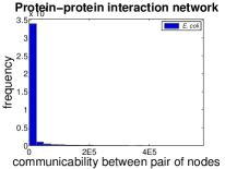
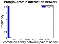
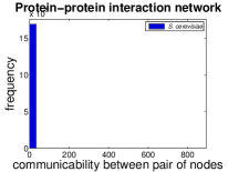
(a)                                         (b)                                         (c)

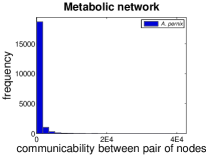
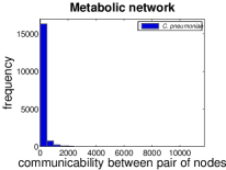
(d)                                         (e)                                         (f)

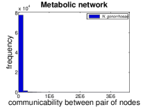
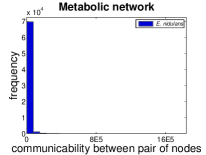
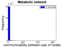
(g)                                         (h)                                         (i)

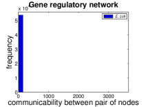
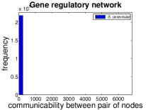
(j)                                       (k)

Figure 3: Histogram of communicability. Here the figures are the histogram of communicability (see equ 2.0.1) of protein-protein interaction networks, metabolic networks and gene regulatory networks. X-axis represent communicability between pair of nodes in a network and Y-axis represents frequency. Protein-protein interaction networks: (a) E. Coli, (b) S. cerevisiae, (c) H. Pylori, Metabolic networks: (d) A. pernix, (e) A. fulgidus, (f) C. pneumoniae, (g) N. gonorrhoeae, (h) E. nidulans, (i) S. cerevisiae, Gene regulatory networks: (j) E. coli, (k) S. cerevisiae.

Table 2: Z-score of small-world-ness of a network. Here, $n$, $m$ are the number of nodes and edges in a network $G$ respectively. $L_{G}$ is the average shortest path length and $T_{G}$ is the transitivity of $G$. Small-world-ness is given by $SW_{G}$. Z-score of small-world-ness is represented by $Z_{G}$, which is computed over a set of networks have the same number of nodes and degree sequence as $G$ has.

Network ${G}$	$\,\,\,\,n\,\,\,\,$	$\,\,\,\,m\,\,\,\,$	$\,\,\,\,L_{G}\,\,\,\,$	$\,\,\,\,T_{G}\,\,\,\,$	$\,\,\,\,SW_{G}\,\,\,\,$	$\,\,\,\,Z_{G}\,\,\,\,$
Neuronal networks
macaque visual cortex	32	194	1.6593	0.5812	1.4715	10.2856
macaque visual and sensorimotor area	47	313	1.8501	0.5472	1.7914	14.2038
macaque cortical connectivity	71	438	2.2447	0.4418	2.1872	16.9169
cat cortex (complete)	95	1170	1.8645	0.4891	1.7389	15.7985
cat cortex connectivity	52	515	1.6357	0.5850	1.4940	18.1573
C. elegans neuronal network	297	2418	2.4553	0.1807	3.6338	19.3799
Food webs
Ythan Estuary	135	596	2.4135	0.1420	3.0227	-0.1597
Little Rock Lake	183	2434	2.1466	0.3323	2.1125	-1.0949
Grassland	88	137	3.9924	0.1664	4.5413	4.3507
Silwood Park	135	365	3.3887	0.0314	6.5290	0.2847
St Marks Seagrass	49	223	2.0876	0.1896	1.4011	0.5451
St Martin	45	224	1.9333	0.2263	1.3833	0.4440
Protein-protein interaction networks
E. coli	270	716	2.7450	0.1552	10.0457	8.7941
S. cerevisiae	1846	2203	4.2494	0.0550	100.5855	37.1999
H. Pylori	724	1403	3.9931	0.0152	3.5092	-5.3138
Metabolic networks
A. pernix	201	548	2.9597	0.1005	4.0823	2.9362
A. fulgidus	493	1402	3.1839	0.0668	6.7729	2.7412
C. pneumoniae	187	435	3.2643	0.1131	4.8712	4.9490
N. gonorrhoeae	399	1185	2.8778	0.0737	6.0026	1.9721
E. nidulans	377	1074	3.0405	0.0789	6.1203	4.6917
C. elegans	452	1332	3.1013	0.0710	7.8039	5.0742
Gene regulatory networks
E. coli	328	456	4.8337	0.0243	3.3048	-3.4238
S. cerevisiae	662	1062	5.1995	0.0163	3.5882	-6.0691

.

References

- [1] Albert-László Barabási and Réka Albert 1999. Emergence of Scaling in Random Networks, Science 286 (5439), 509-512.
- [2] Noga Alon 1986. Eigenvalues and expanders, Combinatorica 6 (2), 83-96.
- [3] J. Ignacio Alvarez-Hamelin, Luca Dall’Asta, Alain Barrat and Alessandro Vespignani 2005. Large scale networks fingerprinting and visualization using the k-core decomposition, Advances in neural information processing systems 18, 41-50.
- [4] Norman Biggs 1993. Algebraic Graph Theory, Cambridge University Press, Cambridge.
- [5] Bela Bollobás 1978. Extremal Graph Theory, Academic Press, New York.
- [6] Bela Bollobás 1988. Graph Theory and Combinatorics: Proceedings of the Cambridge Combinatorial Conference in Honor of P. Erdös, Elsevier Science Publishers B.V., Netherlands.
- [7] Gareth Butland, José Manuel Peregrín-Alvarez, Joyce Li, Wehong Yang, Xiaochun Yang, Veronica Canadien, Andrei Starostine, Dawn Richards, Bryan Beattie, Nevan Krogan, Michael Davey, John Parkinson, Jack Greenblatt and Andrew Emili 2005. Interaction network containing conserved and essential protein complexes in Escherichia coli, Nature 433, 531-537.
- [8] Shai Carmi, Shlomo Havlin, Scott Kirkpatrick, Yuval Shavitt and Eran Shir 2007. A model of Internet topology using k-shell decomposition, PNAS 104 (27), 11150-11154.
- [9] Fan R. K. Chung 1997. Spectral Graph Theory, AMS.
- [10] Paul Erdös and Alfréd Rényi 1959. On random graphs I., Publicationes Mathematicae Debrecen 6, 290-297.
- [11] Paul Erdös and Alfréd Rényi 1960. On the Evolution of random graphs, Bulletin of the International Statistical Institute 38 (4), 343-347.
- [12] Ernesto Estrada and Naomichi Hatano 2008. Communicability in complex networks, Phys. Rev. E 77 (3), 036111.
- [13] Ernesto Estrada 2006. Spectral scaling and good expansion properties in complex networks, Europhys. Lett. 73, 649-655.
- [14] Illés J. Farkas, Imre Derényi, Albert-László Barabási and Tamas Vicsek 2001. Spectra of ”real-world” graphs: Beyond the semicircle law, Phys. Rev. E 64, 026704.
- [15] I. Farkas, I. Derényi, H. Jeong, Z. Néda, Z.N. Oltvai, E. Ravasz, A. Schubert, A.-L. Barabási and T. Vicsek 2002. Networks in life: scaling properties and eigenvalue spectra, Physica A 314, 25-34.
- [16] Mark D. Humphries and Kevin Gurney 2008. Network ’small-world-ness’: a quantitative method for determining canonical network equivalence, PLoS ONE 3 (4), e0002051.
- [17] I.Ispolatov, P.L.Krapivsky and A.Yuryev 2005. Duplication-divergence model of protein interaction network, Phys Rev E Stat Nonlin Soft Matter Phys 71 (6), 061911.
- [18] H. Jeong, B. Tombor, R. Albert, Z. N. Oltvai and A.-L. Barabási 2000. The large-scale organization of metabolic networks, Nature 407, 651-654.
- [19] Maksim Kitsak, Lazaros K. Gallos, Shlomo Havlin, Fredrik Liljeros, Lev Muchnik, H. Eugene Stanley and Hernán A. Makse 2010. Identification of influential spreaders in complex networks, Nature Physics 6, 888-893.
- [20] R. Milo, S. Shen-Orr, S. Itzkovitz, N. Kashtan, D. Chklovskii and U. Alon 2002. Network Motifs: simple building blocks of complex networks, Science 298 (5594), 824–827.
- [21] M. E. J. Newman 2010. Networks: An Introduction, Oxford University Press.
- [22] M. E. J. Newman 2003. The structure and function of complex networks. SIAM Review 45 (2), 167-256.
- [23] Mikail Rubinov and Olaf Sporns 2010. Complex network measures of brain connectivity: Uses and interpretations. NeuroImage 52, 1059-1069.
- [24] Peter Sarnak 2004. What is an expander?, Notices of the AMS 51 (7), 762-763.
- [25] Stephen B. Seidman 1983. Network structure and minimum degree, Social Networks 5 (3), 269-287.
- [26] R. Michael Tanner 1984. Explicit concentrators from generalized N-gons, SIAM. J. on Algebraic and Discrete Methods 5 (3), 287-293.
- [27] Duncan J. Watts and Steven H. Strogatz 1998. Collective dynamics of ’small-world’ networks, Nature 393, 440-442.
- [28] J. G. White, E. Southgate, J. N. Thomson and S. Brenner 1986. The structure of the nervous-system of the Nematode Caenorhabditis elegans, Philos Trans R Soc Lond Ser B Biol Sci 314 (1165), 1–340.
- [29] Omer Reingold, Salil Vadhan, and Avi Wigderson 2002. Entropy waves, the zig-zag graph product, and new constant-degree expanders, Annals of Mathematics 155, 157-187.