Blind deconvolution of density-matrix renormalization-group spectra

Abstract

We present a numerical method for calculating piecewise smooth spectral functions of correlated quantum systems in the thermodynamic limit from the spectra of finite systems computed using the dynamical or correction-vector density-matrix renormalization group method. The key idea is to consider this problem as a blind deconvolution with an unknown kernel which causes both a broadening and finite-size corrections of the spectrum. In practice, the method reduces to a least-square optimization under non-linear constraints which enforce the positivity and piecewise smoothness of spectral functions. The method is demonstrated on the single-particle density of states of one-dimensional paramagnetic Mott insulators represented by the half-filled Hubbard model on an open chain. Our results confirm that the density of states has a step-like shape but no square-root singularity at the spectrum onset.

I Introduction

The dynamical density–matrix renormalization group (DMRG) jec00 ; jec02 and the closely related correction–vector DMRG kue99 ; pat99 have been widely used in the last decade to compute the dynamical correlation functions and spectral functions of low-dimensional strongly correlated quantum systems. jec08a ; jec08b Although more powerful DMRG approaches have been developed recently, whi08 ; wei09 ; hol11 ; dar11 dynamical DMRG (DDMRG) often remains the method of choice because it offers two practical advantages over the other approaches: it is simpler and it can be easily parallelized. For instance, it has been recently shown that DDMRG allows us to investigate features with small spectral weights such as power-law pseudo-gaps in Luttinger liquids. jec13 The main drawback of DDMRG is that it always yields the convolution of the desired spectrum with a Lorentzian distribution of finite width. Therefore, the true spectrum can only be obtained through a deconvolution of the DDMRG spectrum. (In principle, there are some methods to get around this problem kue99 ; pet11 but they are rarely used in practice.)

Deconvolution is a typical ill-conditioned inverse problem, however. nr ; ole09 A direct solution of the deconvolution equation usually yields a very noisy and thus useless spectrum. Nevertheless, various regularization methods have been successfully used to deconvolve DDMRG spectra for one-dimensional systems and quantum impurity problems. wei09 ; geb03 ; nis04a ; nis04b ; raa04 ; raa05 ; jec07 ; sch10 ; ulb10 Astonishingly, some of these deconvolution methods even allow us to bypass the finite-size scaling analysis and to obtain the piecewise smooth spectrum of an infinite systems directly from a broadened finite-system DDMRG spectrum. Unfortunately, regularization also smooths out the sharp features of the true spectrum. This is a serious issue as the spectra of one-dimensional systems and quantum impurities often exhibit very interesting (power-law) singularities.

In this paper we present a method, which allows us to determine sharp spectral features in the thermodynamic limit starting from a broadened finite-system DDMRG spectrum. For this purpose we consider the extrapolation to the thermodynamic limit and the deconvolution for the Lorentzian kernel to be a single blind deconvolution, ole09 ; cam07 i. e. an inverse problem with an unknown kernel including both the Lorentzian broadening and the finite-size effects. The key idea to preserve sharp spectral features in a piecewise smooth spectrum is to impose a minimal distance $d$ between extrema of the deconvolved spectrum. To illustrate our method we investigate the single-particle density of states (DOS) of one-dimensional paramagnetic Mott insulators represented by the half-filled Hubbard model. hub63 We confirm that this DOS has the step-like onset predicted by field-theoretical studies ess02 at least at weak to intermediate coupling up to $U=8t$.

II Model and observable

The Hubbard model hub63 with on-site interaction $U\geq 0$ and nearest-neighbor hopping $t$ is a basic lattice model for the physics of strongly interacting electrons, in particular the Mott metal-insulator transition. mot90 ; geb97 At half filling (i. e., the number of electrons equals the number of sites $N$) the ground state is a Mott insulator for strong interaction $U/t$, while it is a Fermi gas in the non-interacting limit $U=0$. The Hamiltonian of the Hubbard model is defined by

$$H = -t\sum_{\langle ij\rangle,\sigma}\left(c^{\dagger}_{i,\sigma}c^{\phantom{\dagger}}_{j,\sigma}+c^{\dagger}_{j,\sigma}c^{\phantom{\dagger}}_{i,\sigma}\right)-\mu\sum_{i}n_{i}$$ (1)

$$+U\sum_{i}n_{i,\uparrow}n_{i,\downarrow}$$

where the operator $c^{\dagger}_{i,\sigma}$ ($c^{\phantom{\dagger}}_{i,\sigma}$) creates (annihilates) an electron with spin $\sigma$ on the site $i$, $n_{i,\sigma}=c^{\dagger}_{i,\sigma}c^{\phantom{\dagger}}_{i,\sigma}$, and $n_{i}=n_{i,\uparrow}+n_{i,\downarrow}$. The first sum runs over all pairs $\langle ij\rangle$ of nearest-neighbor sites while the other two sums run over all sites $j$. Here we will only consider half-filled systems and thus set the chemical potential $\mu=\frac{U}{2}$ to have electron-hole-symmetric spectra and a Fermi energy $\epsilon_{\rm F}=0$.

The bulk single-particle DOS $D(\epsilon)$ can be measured experimentally using photoemission spectroscopy or scanning tunneling spectroscopy. Theoretically, it can be defined as the average of the local DOS

$$D(\epsilon)=\frac{1}{2N}\sum_{j,\sigma}D_{\sigma}(j,\epsilon)$$ (2)

where the sum runs over both spins and all sites $j$ in the lattice, while $D_{\sigma}(j,\epsilon)$ is the local single-particle DOS at site $j$ for spin $\sigma$ and can be calculated using

$$D_{\sigma}(j,\epsilon)=\sum_{n}|\langle n|c^{\dagger}_{j,\sigma}|0\rangle|^{2}\ \delta(\epsilon-E_{n}+E_{0})$$ (3)

for $\epsilon\geq 0$ and

$$D_{\sigma}(j,\epsilon)=\sum_{n}|\langle n|c_{j,\sigma}|0\rangle|^{2}\ \delta(\epsilon+E_{n}-E_{0})$$ (4)

for $\epsilon\leq 0$. Here $|n\rangle$ denotes the eigenstates of the Hamiltonian $H$ and $E_{n}$ their eigenenergies in the Fock space. The ground state for the chosen number of particles corresponds to $n=0$. The total spectral weight is

$$\int_{-\infty}^{+\infty}d\epsilon\ D_{\sigma}(j,\epsilon)=1.$$ (5)

We will consider only lattice geometry for which the Hamiltonian (1) is invariant under the electron-hole transformation $c^{{\dagger}}_{j,\sigma}\leftrightarrow\pm c^{\phantom{{\dagger}}}_{j,\sigma}$. Therefore, for half filling the density of states is symmetric, $D_{\sigma}(j,\epsilon)=D_{\sigma}(j,-\epsilon)$. If the system is translation invariant, the bulk DOS and the local DOS are identical. For DMRG simulations, however, open boundary conditions are preferred to periodic boundary conditions. In this case, the bulk DOS can be identified with the local DOS on one of the two equivalent middle sites of the system, i. e. as far as possible from the system boundaries. jec13

III Deconvolution

Inverse problems such as (blind) deconvolutions nr ; ole09 occur in many scientific fields and are among the most challenging numerical computations. Experimental measurements and computer simulations often yield approximations of the true quantities which are measured or computed, respectively. It is often assumed that the deviations from exact results can be modelled by a convolution with a smoothing function and an additive noise due to the finite accuracy and resolution of the measurement or simulation process. A typical example of a blind deconvolution is the reconstruction of an original signal from a degraded copy using incomplete information about the degradation process. ole09 ; cam07 Here we want to compute sharp spectral features in the piecewise smooth spectrum of an infinite system from a broadened finite-system spectrum calculated with DDMRG. In this section we first show that this task can be formulated as a blind deconvolution problem, then present an algorithm for solving it.

III.1 Blind deconvolution problem

Let $S^{(N)}(\epsilon)$ be a spectrum of a finite lattice model with $N$ sites. This spectrum is a Dirac-comb (a finite sum of Dirac-peaks)

$$S^{(N)}(\epsilon)=\sum_{n}S^{(N)}_{n}\ \delta\left(\epsilon-E^{(N)}_{n}\right)$$ (6)

where the sum runs over all Hamiltonian eigenstates $|n\rangle$ which contributes to the spectrum, i. e. with a nonzero spectral weight $S^{(N)}_{n}$. Here $E^{(N)}_{n}$ denotes the corresponding excitation energies. This spectrum can be broadened with a Lorentzian distribution of width $\eta$

$$L_{\eta}(\epsilon)=\frac{1}{\pi}\frac{\eta}{\epsilon^{2}+\eta^{2}}$$ (7)

to obtain a smooth spectral function

$$S^{(N)}_{\eta}(\epsilon) = \int d\omega\ S^{(N)}(\omega)\ L_{\eta}(\epsilon-\omega)$$ (8)

$$= \frac{1}{\pi}\sum_{n}S^{(N)}_{n}\frac{\eta}{\left(\epsilon-E^{(N)}_{n}\right)^{2}+\eta^{2}}.$$

With the DDMRG method we can calculate this spectrum for a discrete set of excitation energies $\{\epsilon_{\alpha};\alpha=1,\dots,M\}$. As numerical calculations are always affected by errors, DDMRG actually yields values $W^{(N)}_{\eta}(\epsilon_{\alpha})$ which are related to the true spectral function by

$$W^{(N)}_{\eta}(\epsilon_{\alpha})=S^{(N)}_{\eta}(\epsilon_{\alpha})+X_{\alpha}$$ (9)

for $\alpha=1,\dots,M$, where $X_{\alpha}$ represents the unknown errors. (It should be noted that DDMRG errors $X_{\alpha}$ include significant systematic contributions, for instance due to the variational nature of the procedure. jec02 ) In principle, one could determine the true spectrum, i. e., the excitation energies $E^{(N)}_{n}$ and the corresponding weights $S^{(N)}_{n}$, through this system of equations. In practice, however, this is an ill-conditioned problem except for simple discrete spectra. Moreover, we are not interested in resolving the discrete peaks of small systems but in calculating the piecewise smooth spectra of macroscopic systems.

The spectrum in the thermodynamic limit is given by

$$S(\epsilon)=\lim_{\eta\rightarrow 0}\lim_{N\rightarrow\infty}S^{(N)}_{\eta}(\epsilon).$$ (10)

Note that, generally, the order of the two limits can not be exchanged. Typically, the spectral function $S(\epsilon)$ is piecewise smooth, i. e., it exhibits one or more continua as well as isolated sharp features such as steps, power-law singularities or cusps. In principle, one should carry out several DDMRG simulations with varying system size $N$ and broadening $\eta$ and then extrapolate the numerical data to obtain $S(\epsilon)$. In most cases, a simultaneous extrapolation for $N\rightarrow\infty$ and $\eta\rightarrow 0$ is possible jec02 using a constant value of $\eta N$. Nevertheless, the computational cost of DDMRG simulations increases very rapidly with smaller $\eta$ and the overall cost of this approach is prohibitive for a full spectrum. Indeed, this approach has been mostly used to study isolated spectral features in the thermodynamic limit such as power-law singularities and steps. jec02 ; jec08b ; jec13

As all operations used to define $S(\epsilon)$ from $S^{(N)}_{\eta}(\epsilon)$ are linear, the broadened spectrum of the finite system can also be written explicitly as a function of the infinite system spectrum

$$S^{(N)}_{\eta}(\epsilon)=\int_{-\infty}^{\infty}d\omega\ K^{(N)}_{\eta}(\epsilon,\omega)\ S(\omega).$$ (11)

The kernel $K^{(N)}_{\eta}(\epsilon,\omega)$ includes both the finite-size effects and the Lorentzian smoothing. Its form is not known but it is clear that we must recover a pure Lorentzian smoothing in the thermodynamic limit

$$\lim_{N\rightarrow\infty}K^{(N)}_{\eta}(\epsilon,\omega)=L_{\eta}(\epsilon-\omega).$$ (12)

Combining eqs. (9) and (11) we obtain a system of equations

$$W^{(N)}_{\eta}(\epsilon_{\alpha})=\int_{-\infty}^{\infty}d\omega\ K^{(N)}_{\eta}(\epsilon_{\alpha},\omega)\ S(\omega)+X_{\alpha}$$ (13)

for $\alpha=1,\dots,M$, relating the DDMRG data set

$$\left\{\left(\epsilon_{\alpha},W^{(N)}_{\eta}(\epsilon_{\alpha})\right);\alpha=1,\dots,M\right\}$$ (14)

to the infinite system spectrum $S(\epsilon)$.

Determining $S(\epsilon)$ from these equations is a so-called inverse problem. nr This kind of problem is also called blind deconvolution since our knowledge of the kernel is incomplete. [Strictly speaking, it is not a deconvolution because eq. (13) is not a convolution. However, as the kernel approaches the form $K^{(N)}_{\eta}(\epsilon,\omega)=L_{\eta}(\epsilon-\omega)$ in the thermodynamic limit, we will use the terminology of deconvolution problems.] It should be obvious that this is an ill-posed problem. First, the errors $X_{\alpha}$ and the kernel $K^{(N)}_{\eta}(\epsilon,\omega)$ are not known. Second, the problem is sorely underdetermined as we try to reconstruct the function of a continuous variable from a finite number $M$ of data points. Finally, a convolution with a Lorentzian is a smoothing operation and thus the corresponding deconvolution is an extremely ill-conditioned inverse problem: the solution will be extremely sensitive to small changes or errors in the input.

III.2 Cost function approach

Various deconvolution methods have been used successfully to deduce piecewise smooth spectra from the broadened finite-system spectra calculated with DDMRG. They include, direct inversion at low resolution, geb03 linear regularization methods, nis04a ; jec07 Fourier transform with low-pass filtering, raa04 ; raa05 nonlinear regularization methods such as the Maximum Entropy Method, raa05 parametrization with piecewise polynomial functions, wei09 ; raa05 and a deconvolution ansatz for the self energy. sch10 ; ulb10 However, this task has not been viewed as a blind deconvolution so far. Instead, it has been considered as the deconvolution of a perfectly known kernel. The need for regularization or filtering techniques has been viewed as the consequence ill-conditioning and under-determination of the problem (13) with a Lorentzian kernel.

All of these methods offer some advantages for particular spectral forms. However, their common drawback is that they are ill-suited for sharp spectral features, such as steps or power-law singularities, within or at the edge of a continuum. Either the regularization procedure smooths out true sharp features excessively or it allows the occurrence of deconvolution artifacts (artificial sharp structures, rapid oscillations or negative spectral weight), especially in the vicinity of the true spectrum singularities. Naturally, better results can be obtained if we can use a priori knowledge about the properties of the spectrum whi08 ; raa05 but, in practice, this is a rare occurrence. Therefore, we need a better method for solving the inverse problem (13) which allows us to determine isolated sharp spectral features accurately while preserving the positivity and the piecewise smoothness of $S(\epsilon)$.

Let the DDMRG data (14) be evenly distributed in the energy interval $[\epsilon_{A},\epsilon_{B}]$. The difference between two consecutive energies is $\Delta\epsilon\sim 1/M$. Additionally, consider a set of equidistant energies $\{\omega_{\mu};\mu=1,\dots,L\}$ in the interval $[\omega_{A},\omega_{B}]\subset[\epsilon_{A},\epsilon_{B}]$. The distance between these energies is $\Delta\omega\sim 1/L$. As we will always use $L\geq M$, we have $\Delta\omega\leq\Delta\epsilon$. (Typical values are $M\approx 10^{2}-10^{3}$ and $L\approx 10^{3}-10^{4}$.) As in a least-square approach we define a cost function $\chi\left(\{R_{\mu}\}\right)$ as the sum of the squares of the differences between the DDMRG data and an approximate representation parametrized by a discrete set of variables $\{R_{\mu};\mu=1,\dots,L\}$

$$\chi=\sum_{\alpha=1}^{M}\left(W^{(N)}_{\eta}(\epsilon_{\alpha})-\sum_{\mu=1}^{L}K^{(N)}_{\eta}(\epsilon_{\alpha},\omega_{\mu})R_{\mu}\Delta\omega\right)^{2}.$$ (15)

The absolute minimum of $\chi\left(\{R_{\mu}\}\right)$ is zero and the corresponding parameters $\{R_{\mu}\}$ are determined by a linear system of $M$ equations

$$W^{(N)}_{\eta}(\epsilon_{\alpha})=\sum_{\mu=1}^{L}K^{(N)}_{\eta}(\epsilon_{\alpha},\omega_{\mu})R_{\mu}\Delta\omega.$$ (16)

Using this equation system to determine the parameters $\{R_{\mu}\}$ would be an unconstrained least-square fit.

In the limit $L\rightarrow\infty$ (followed by $\epsilon_{A}\rightarrow-\infty$ and $\epsilon_{B}\rightarrow+\infty$) this equation system becomes equivalent to the inverse problem (13) with vanishing errors $X_{\alpha}=0$. Thus the absolute minimum of $\chi\left(\{R_{\mu}\}\right)$ yields the spectrum $S(\epsilon)$ through

$$R_{\mu}=S(\omega_{\mu}).$$ (17)

If we substitute a Lorentz kernel $L_{\eta}(\epsilon_{\alpha}-\omega_{\mu})$ for the unknown kernel, $K^{(N)}_{\eta}(\epsilon_{\alpha},\omega_{\mu})$ in (16), we recover the finite-system deconvolution problem defined by equations (8) and (9) for vanishing errors $X_{\alpha}$. Thus the absolute minimum of the cost function corresponds to the discrete finite-system spectrum $S^{(N)}(\epsilon)$ through $R_{\mu}\Delta\omega=S^{(N)}_{n}$ if $\omega_{\mu}=E^{(N)}_{n}$ and $R_{\mu}=0$ otherwise. Physically, the solution of the deconvolution problem is unique for vanishing errors $X_{\alpha}$ and thus the cost function should have a unique absolute minimum. From a mathematical point of view, however, the equation system (16) could have no solution or infinitely many solutions. Then any small error $X_{\alpha}$ can generate wildly different (and mostly unphysical) solutions.

Therefore, as (12) holds in the thermodynamic limit, it is possible and preferable to obtain a reasonable approximation of the infinite-system spectrum $S(\epsilon)$ from the minimization of the cost function (15) with a Lorentz kernel under the constraint that the spectral function $S(\epsilon)$ is physically allowed. For instance, $S(\epsilon)$ should be positive semidefinite and piecewise smooth. Generally, this solution does not correspond to the absolute minimum or even a local minimum of $\chi\left(\{R_{\mu}\}\right)$. Indeed, the solution of the inverse problem (13) corresponds to the value

$$\chi\left(\{R_{\mu}\}\right)=\sum_{\alpha=1}^{M}X_{\alpha}^{2}$$ (18)

if we assume that the relation (17) holds. Of course, it could be possible to lower the cost function with other configurations $\{R_{\mu}\}$ but in that case the relation (17) would no longer hold. Note that, this idea has been implicitly assumed in all previous deconvolution schemes of DDMRG data aiming at piecewise smooth spectra so far. However, in these approaches the agreement between solution $\{R_{\mu}\}$ and numerical data $\{W^{(N)}_{\eta}(\epsilon_{\alpha})\}$ in eq. (16) with a Lorentzian kernel is considered essential while the regularization of the solution and the errors $X_{\alpha}$ are seen as perturbations which should deteriorate the agreement as little as possible.

Yet a blind deconvolution requires equal balancing of the agreement between solution and numerical data and of the smoothness and stability of the solution. cam07 Hence we must take a different point of view: The Lorentzian kernel (12) is only an approximation of the true kernel $K^{(N)}_{\eta}(\epsilon,\omega)$ and the physical constraints on the deconvolved spectrum $S(\epsilon)$ are essential in the minimization of the cost function. Thus we accept significant deviations of $\{R_{\mu}\}$ from the conditions (16) yielding the absolute minimum of the cost function, or, equivalently, we assume that the errors $X_{\alpha}$ can be substantial.

III.3 Method

Therefore, the blind deconvolution problem can be formulated as a least-square optimization under non-linear constraints. We want to minimize the cost function (15) with the Lorentz kernel under the constraints that the spectrum $S(\epsilon)$ has the following properties:

1. finite band width, i.e $S(\omega)=0$ for all $\omega<\omega_{A}$ and all $\omega>\omega_{B}$ for some finite $\omega_{A,B}$,

2. positive semi-definite, $S(\epsilon)\geq 0$, and

3. piecewise smooth.

The first two conditions are easily expressed for the parameters $\{(\omega_{\mu},R_{\mu})\}$. The somewhat fuzzy concept of a piecewise smooth spectrum must now be formulated more precisely. In principle, we wish that $S(\epsilon)$ is piecewise continuous and that the distance between discontinuities is larger than a minimal energy difference $d$. As we must work with a finite number $L$ of points $(\omega_{\mu},R_{\mu})$, we only have a discrete representation of $S(\epsilon)$ and we have to formulate a “continuity” condition for the discrete set of variables as well. Therefore, we require that the distance between two significant extrema is larger than a parameter $d>0$. Two neighboring extrema at energy $\epsilon_{1}$ and $\epsilon_{2}$ are significant if there relative height difference is larger than a parameter $h\geq 0$,

$$2\frac{|S(\epsilon_{1})-S(\epsilon_{2})|}{S(\epsilon_{1})+S(\epsilon_{2})}>h.$$ (19)

This condition can easily be formulated for the parameters $\{(\omega_{\mu},R_{\mu})\}$. The minimal extremum distance $d$ must be chosen carefully. It should be smaller than the distance between actual singularities in the spectrum $S(\epsilon)$ but a too small value allows many artificial peaks in a deconvolved spectrum. In practice, we have found that we can obtain reasonable solutions to the blind deconvolution problem which look piecewise smooth using $d\gtrsim\eta$. In all examples discussed in this paper every local extremum is considered to be significant (i. e., we have used the precision of floating-point arithmetic $h\approx 10^{-16}$).

The cost function is minimized iteratively. Iterations are repeated until the procedure converges. Each iteration consists in two steps. In the first step the cost function $\chi(\{R_{\mu}\})$ is minimized with respect to each variable $R_{\mu}\geq 0$ successively. This minimization under constraint does not present any difficulty as $\chi(\{R_{\mu}\})$ is a second-order polynomial in each variable $R_{\mu}$. In the second step, we first find the positions $(\omega_{\nu},\omega_{\tau})$ of all significant extrema pairs in $\{(\omega_{\mu},R_{\mu})\}$ which are separated by less than a distance $d$. Then we interpolate the data $\{(\omega_{\mu},R_{\mu})\}$ linearly from $\mu=\nu-1$ to $\mu=\tau+1$ to smooth out the spectrum around the extrema. In doing so we take care to preserve the total spectral weight

$$S=\sum_{\mu=1}^{L}R_{\mu}\Delta\omega\approx\int_{-\infty}^{+\infty}d\epsilon\ S(\epsilon).$$ (20)

The search for extrema and their smoothing is repeated until there is no more close significant extrema in $\{(\omega_{\mu},R_{\mu})\}$. Then we start the next iteration. By design the first step results in a decrease of $\chi(\{R_{\mu}\})$. The second step nearly always results in an increase of $\chi(\{R_{\mu}\})$. Without the second step, however, we would perform an under-determined ($L\gg M$) deconvolution devoid of any regularization mechanism and thus obtain a completely useless result. Typically, we observe a rapid and monotonic decrease of $\chi(\{R_{\mu}\})$ in the initial iterations followed by a saturation or oscillations in further iterations. Therefore, we monitor the changes in the parameters $R_{\mu}$ and the normalized cost function

$$\theta^{2}=\frac{\chi}{S^{2}M}$$ (21)

to determine converged configurations $\{R_{\mu}\}$. Convergence requires typically $10^{2}$ to $10^{3}$ iterations depending on the quality of the DDMRG data and the complexity of the spectrum. Finally, the solution $\{(\omega_{\mu},R_{\mu})\}$ can be smoothened using a narrow Lorentzian distribution to obtain a continuous function

$$S(\epsilon)=\sum_{\mu=1}^{L}R_{\mu}L_{\tilde{\eta}}(\epsilon-\omega_{\mu})$$ (22)

with ${\tilde{\eta}}\ll\eta$. Alternatively, we can use a Gaussian distribution wei09 of width $\sigma\ll\eta$. The second approach yields sharper (real or artificial) features because the tail of a Gaussian distribution decreases faster than that of the Lorentz distribution. As our minimization problem possesses many local minima, the final results $\{R_{\mu}\}$ depend somewhat on the criteria for convergence. However, if the final smoothening function is broad enough, the differences are canceled out. If the DDMRG data (14) are not evenly distributed in the interval $[\epsilon_{A},\epsilon_{B}]$ or if they already exhibit numerous close extrema, it is useful to regularize them before starting the deconvolution iterations using an interpolation and the smoothening procedure described above.

The computational effort required by this procedure is negligible compared to the computational cost of the DDMRG simulations yielding the original data. (Our code in the programming language C contains less than 400 lines of instructions and the deconvolution of one spectrum takes less than 30 minutes on a single CPU.) Therefore, we have not bothered to optimize the algorithm. Nevertheless, it should be implemented in such a way that it only requires $\sim L^{2}$ operations rather than the $\sim L^{3}$ operations of a straightforward implementation.

The method described here can be generalized in several ways. For instance, it is possible to use a variable spacing $\Delta\epsilon$ of the DDMRG data points, such as a finer mesh close to sharp spectrum features. However, this does not seem to improve the results in practice because the broadening parameter $\eta$, not $\Delta\epsilon$, is the limiting scale. A generalization to variable $\eta$ and $\Delta\epsilon$, as proposed in Ref. nis04a, for quantum impurity problems, should also be possible but we have not tested it yet. To introduce information about the variation of the spectrum with $\eta$ one could combine DDMRG data obtained for different values of $\eta$ by defining an overall cost function as the sum of the cost functions for each $\eta$. These generalizations will be tested in future works.

IV DOS of one-dimensional Mott insulators

As an illustration of our deconvolution procedure we discuss its application to the DOS of one-dimensional paramagnetic Mott insulators. The nature of Mott insulators is a long-standing open problem in the theory of strongly correlated quantum systems. mot90 ; geb97 In a paramagnetic Mott insulator quantum fluctuations or frustration of the antiferromagnetic spin exchange coupling prevents the formation of a long-range magnetic order. Experimentally, non-magnetic Mott insulators have been found in layered organic insulators kur05 as well as in quasi-one-dimensional cuprate chains kim04 and ladders azu94 . Despite decades of extensive research the properties of Mott insulators, in particular their single-particle DOS, are still poorly understood and thus actively investigated. The half-filled Hubbard model hub63 with repulsive on-site interaction $U\geq 0$ is a basic lattice model for describing Mott insulators and the Mott metal-insulator transition. Here we consider the case of the one-dimensional Hubbard model, which is exactly solvable by Bethe Ansatz. lie68 ; hubbard-book At half- filling it describes a paramagnetic Mott insulator with a charge gap (Mott-Hubbard gap) $2\Delta>0$ for $U>0$. However, the DOS cannot be calculated directly from the Bethe Ansatz.

All DDMRG spectra used here have been calculated with a variable number of density-matrix eigenstates kept (up to 512) to reach a discarded weight lower than $10^{-4}$ and to check DMRG truncation errors. Typically, convergence was reached after three sweeps for each frequency interval of size $\eta$. The DDMRG method is presented in detail in Ref. jec02, .

For $U=0$ the exact DOS of the tight-binding chain in the thermodynamic limit is

$$D_{\text{tb}}(\epsilon)=\frac{1}{\pi}\frac{1}{\sqrt{4t^{2}-\epsilon^{2}}}$$ (23)

for $|\epsilon|<2t$ while $D_{\text{tb}}(\epsilon)$ vanishes for larger $|\epsilon|$. For finite coupling $U$ the spectrum consists in two symmetric Hubbard bands separated by the gap $2\Delta$. Low-order strong-coupling perturbation theory scpt1 ; scpt2 predicts a square-root divergence at the DOS threshold for $U\gg 4t$, namely

$$D_{\text{scpt}}(\epsilon)=\frac{1}{2}D_{\text{tb}}\left(|\epsilon|-\frac{U}{2}\right)$$ (24)

for $\left||\epsilon|-\frac{U}{2}\right|<2t$ and $D_{\text{scpt}}(\epsilon)=0$ otherwise with $\Delta=\frac{U}{2}-2t$. Because of this strong-coupling result and the result of the Hartree-Fock (HF) approximation it has often been assumed that the DOS of one-dimensional Mott insulators exhibits a square-root divergence at the spectrum onset $\epsilon=\pm\Delta$ like in a one-dimensional band insulator. Indeed, in the unrestricted HF approximation the one-dimensional half-filled Hubbard model is an antiferromagnetic Mott insulator for $U>0$. Its DOS is given by

$$D(\epsilon)=\frac{1}{\pi}\frac{\epsilon}{\sqrt{\left(\epsilon^{2}-\Delta_{\text{HF}}^{2}\right)\left(4t^{2}+\Delta_{\text{HF}}^{2}-\epsilon^{2}\right)}}$$ (25)

for $\Delta_{\text{HF}}<|\epsilon|<\sqrt{4t^{2}+\Delta_{\text{HF}}^{2}}$ and vanishes otherwise. Here $2\Delta_{\text{HF}}$ is the HF gap. For $U=0$, $\Delta_{\text{HF}}=0$ and this DOS reduces to the DOS of the tight-biding chain (23). For $U>0$, $\Delta_{\text{HF}}\neq 0$ and the HF DOS shows a square-root divergence at the onset of the spectrum. However, in the weak-coupling limit $U\ll 4t$ a field-theoretical analysis ess02 predicts that the DOS of one-dimensional Mott insulators is constant above the threshold energy $\Delta$,

$$D_{\text{ft}}(\epsilon)=C\ \theta(|\epsilon|-\Delta)$$ (26)

at least for $|\epsilon|\leq 3\Delta\ll 4t$. Thus there is a discrepancy between the field-theoretical and strong-coupling predictions for the behavior of $D(\epsilon)$ just above the threshold energy $\Delta$.

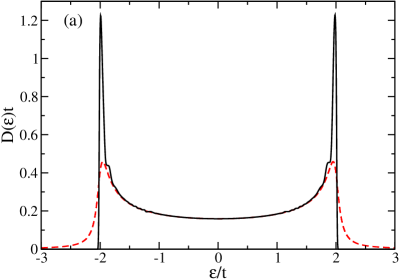
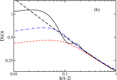
Figure 1: (Color online) DOS of a tight-binding chain: (a) DDMRG spectrum for a $128$-site chain with a Lorentzian broadening $\eta=0.08t$ (red dashed line) and result of our deconvolution method with a Gaussian broadening $\sigma=\eta/10$ (black line). (b) Enlarged view close to the singularity at $\epsilon=2t$ on a double logarithmic scale: Exact results (black long-dashed line), DDMRG data (red short-dashed line), and the deconvolved spectra $\{(\omega_{\mu},R_{\mu})\}$ for $\theta\approx 6\cdot 10^{-4}$ (black solid line) and $\theta\approx 8\cdot 10^{-3}$ (blue dash-dot line).

Figure 1(a) shows the DOS of a tight-binding chain calculated with DDMRG and the result of our deconvolution procedure. The DDMRG spectrum has been calculated in the middle of an open chain with $N=128$ sites using a broadening $\eta=0.08t$, which is just broad enough to hide its discreteness. We see that the square-root divergences at $\epsilon=\pm 2t$ have been smoothed into two broad peaks and that there is substantial spectral weight at energies $|\epsilon|>2t$. The deconvolved DOS has been determined from these same DDMRG data using a minimal extremum distance $d=2\eta=0.16t$ and a final Gaussian broadening with $\sigma=\eta/10=0.008t$. We see now that the singularities at $\epsilon=\pm 2t$ are clearly visible as sharp peaks and that there is not any spectral weight at $|\epsilon|>2t$. Overall the deconvolved DOS is in excellent agreement with the exact spectrum in the thermodynamic limit (23). In particular, we do not observe any unphysical artefact such as negative spectral weight.

However, in fig. 1(a) we observe two shoulders in the deconvolved DOS at energies $\epsilon\approx\pm 1.8t$, which are not present in the exact solution (23). An enlarged view close to the singularity at $\epsilon=+2t$ is shown in fig. 1(b) on a double logarithmic scale. We see that the DDMRG data agree with the exact result only at some distance from the singularity. In this figure we also show deconvolved spectra $\{(\omega_{\mu},R_{\mu})\}$ for two different values of the normalized cost function $\theta$. Clearly, they reproduce the square-root divergence at $\epsilon=+2t$ much better than the original DDMRG data. The overall divergent behavior is visible on a broader energy scale for the smaller value of $\theta$ but we see that the reduction of the cost function is also accompanied by stronger oscillations around the exact result. These oscillations correspond to the shoulder seen in fig. 1(a).

The occurrence of artificial shoulder-like structures is the main drawback of our deconvolution procedure. Any deconvolution method magnifies the noise (numerical errors) which is present in the original data. This the main issue that existing methods try to solve in different ways. wei09 ; geb03 ; nis04a ; nis04b ; raa04 ; raa05 ; jec07 ; sch10 ; ulb10 We have systematically tested our deconvolution procedure using exact results for non-interacting systems and purposely adding random numerical errors. We have found that by preventing the formation of local maxima in the deconvolved spectrum our procedure allows us to control the noise magnification only partially. Unfortunately, it cannot handle extrema ($\equiv$ oscillations) in the spectrum derivative. Thus the magnified noise shows up as shoulder-like structures (but not as local maxima, discontinuities, or sharp angles) on an energy scale $d$ and gives a rough appearance to some deconvoled spectra presented here. In principle, we should be able to correct this deficiency with a higher-order interpolation procedure in the smoothening step or with a smoothening of the derivative of $S(\epsilon)$ (i. e., the finite differences between the parameters $R_{\mu}$). However, we have not yet succeeded in developing a practical algorithm based on these ideas.

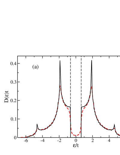
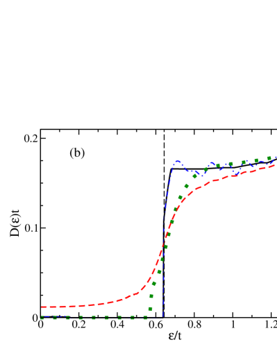
Figure 2: (Color online) (a) DOS of the one-dimensional half-filled Hubbard model at $U=4t$ calculated with DDMRG in a 128-site chain using a broadening $\eta=0.08t$ (red dashed line) and the result of our deconvolution procedure (black line) with a minimal extremum distance $d=2\eta$ and a Gaussian broadening $\sigma=\eta/100$. The vertical dashed lines show the exact position of the DOS threshold calculated from the Bethe Ansatz solution. (b) Enlarged view of the same data around the DOS threshold for $\epsilon>0$. Additionally, the result of our procedure with $d=\eta/2$ (blue dot-dash line) and of a deconvolution with linear regularization nr ; nis04a ; jec07 (green dots) are also shown.

Figure 2(a) shows the single-particle DOS of the half-filled one-dimensional Hubbard model at $U=4t$ calculated with DDMRG and the result of our deconvolution procedure. The DDMRG spectrum has been computed jec08b in the middle of an open chain with $N=128$ sites and a broadening $\eta=0.08t$. The deconvolved spectrum has been obtained from these DDMRG data using a minimal extremum distance $d=2\eta=0.16t$ and a final Gaussian broadening $\sigma=\eta/100=8\cdot 10^{-4}t$. The effects of the broadening are clearly visible in the DDMRG data. For instance, although one can recognize the opening of the Mott-Hubbard gap $2\Delta$, spectral weight is clearly visible inside the gap. A point-wise analysis jec08b of the scaling for $N\rightarrow\infty$ with $\eta N=10.24t$ is required to confirm that the spectral weight jumps from $0$ to a finite value at the onset $\epsilon=\Delta$ and that the gap width agrees with the exact results $E_{c}=2\Delta=1.286t$ calculated with the Bethe Ansatz. lie68 ; hubbard-book However, the behavior for $\epsilon\gtrsim\Delta$ remains uncertain because of the relatively large broadening used in the DDMRG calculation. On the contrary the deconvolved DOS clearly shows a gap with the step-like onset (26) predicted by field theory ess02 at the position $\epsilon=\Delta$ given by the Bethe Ansatz solution. We obtain similarly unambiguous results for $U$ up to $8t$ (see below). Therefore, our numerical investigation confirms the field-theoretical prediction ess02 for the onset of the DOS in one-dimensional Mott insulators.

The superiority of the deconvolved spectrum over the original DDMRG data is even more obvious in fig. 2(b) which shows an enlarged view of the DOS around $\epsilon=\Delta$. In this figure we also show the result of a deconvolution of the DDMRG data with a standard linear regularization method nr ; nis04a ; jec07 . (Note that this method yields negative spectral weights for some energies $\epsilon$ but we show the positive parts only.) We see that the result of the deconvolution procedure proposed in this work is much superior to that of the standard one, which is too blurred to allow us to determine the true form of the DOS at the onset $\epsilon=\Delta$. In addition, fig. 2(b) shows the result of our deconvolution procedure for a minimal extremum distance $d=\eta/2=0.04t$ which is deliberately too small. In that case, artificial oscillations on energy scales $\epsilon\lesssim\eta$ are clearly visible in the deconvolved spectrum.

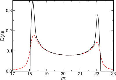
Figure 3: (Color online) Upper Hubbard band in the DOS of the one-dimensional half-filled Hubbard model at $U=40t$ calculated with DDMRG in a 64-site chain using a broadening $\eta=0.16t$ (red dashed line) and the result of our deconvolution procedure (black line) with a Gaussian broadening $\sigma=\eta/100$.

In the strong-coupling limit $U\gg t$ our results are less conclusive. For instance, we show the DDMRG and deconvolved upper Hubbard and for a very strong coupling $U=40t$ in fig. 3. The DDMRG spectrum has been calculated in the middle of an open chain with $N=64$ sites using a broadening $\eta=0.16t$. The deconvolved spectrum has been obtained from these DDMRG data using a minimal extremum distance $d=\eta$ and a final a Gaussian broadening $\sigma=\eta/100$. Two broad peaks are clearly visible at energies $\epsilon\approx\frac{U}{2}\pm 2t$ as predicted for the strong-coupling limit. However, the widths and heights of these peaks after deconvolution are not compatible with the square-root divergences (24) predicted by the low-order strong-coupling expansion. Actually, higher-order corrections indicate scpt1 ; penc that some spectral weight is present below the peak at $\epsilon\approx\frac{U}{2}-2t=18t$ on a scale set by the effective spin exchange coupling $J=4t^{2}/U=0.1t$. This width is compatible with our deconvolved spectra for $U\geq 16t$. Thus our numerical results agree at least qualitatively with strong-coupling perturbation theory and suggest that the square-root divergences in the DOS (24) is an artifact of a truncated strong-coupling expansion.

Nevertheless, for strong coupling such as $U=40t$ we are not able to determine the shape of the DOS at the onset $\epsilon=\Delta$. In particular, it is not clear if the field-theoretical prediction (26) is still valid. Indeed, if the distance $\sim J=4t^{2}/U$ between onset at $\epsilon=\Delta$ and peak at $\epsilon\approx\frac{U}{2}-2t$ becomes smaller than the minimal extremum distance $d$, we can no longer distinguish both structures in the deconvolved spectrum. In practice, the distance $d$ must be comparable to the broadening $\eta$ of the DDMRG data to obtain piecewise smooth spectra. Therefore, although we can reduce the broadening of isolated spectral structures by several orders of magnitude, we cannot resolve distinct spectral features on a scale lower than the original broadening of the DDMRG data. This is a limitation of our deconvolution method that one has to keep in mind.

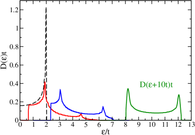
Figure 4: (Color online) Deconvolved DOS of the half-filled Hubbard model for energies $\epsilon>0$ for $U=0$ (dashed line), and from left to right $U/t=4$ (red line), $8$ (blue line) and $40$ (green line). The result for $U=40t$ is shifted to the left by $10t$.

Finally, fig. 4 recapitulates the evolution of the DOS as a function of the interaction strength $U/t$. As the spectrum is symmetric $D(-\epsilon)=D(\epsilon)$, we show only the deconvolved spectra for positive energies (i. e., the upper Hubbard band). At $U=0$ the spectrum consists in a single band with two clearly visible square-root singularities at the band edges $\epsilon=\pm 2t$. For weak coupling $U$ the band splits into two symmetric Hubbard bands separated by a gap $2\Delta$, which agrees perfectly with the charge gap calculated from the Bethe Ansatz solution. At the DOS onsets $\epsilon=\pm\Delta$ the spectrum exhibits the step-like behavior (26) predicted by field theory. ess02 There is an apparent plateau between the onset and a strong first peak, which evolves from the square-root singularities at $\epsilon=\pm 2t$ for $U=0$. Additionally, we observe substantial spectral weight and a small second peak at higher excitation energy. However, for weak enough $U$ most of the spectral weight lies between the spectrum onset and the first peak.

As $U$ increases (compare the spectra for $U=4t$ and $U=8t$ in fig. 4), the spectrum and all its features shift to higher excitation energy and the spectral weight becomes more concentrated between the visible peaks. In addition, we note that the separation between onset energy $\Delta$ and the strong first peak becomes systematically smaller until it is no longer resolvable with our method, the peak separation increases monotonically from about $2t$ for $U\ll t$ to approximately $4t$ for $U\gg t$, and the strength of both peaks become more equal.

Comparing the DOS with the momentum-resolved spectral function and the Bethe Ansatz dispersion (see figs. 4 and 5 in Ref. jec08b, ) we note that the strong first peak corresponds to the edge of the spinon branch at momentum $k=0$, the weak second peak corresponds to the edge of the holon branch at $k=\pm\frac{\pi}{2}$, and the upper edge of the DOS spectrum coincide with the edge of the single spinon-holon continuum. Finally, we do not observe any spectral weight outside the first lower and upper Hubbard bands and these two bands account for the full spectral weight (5). Thus we conclude that higher-energy Hubbard bands do not carry any spectral weight in the bulk single-particle DOS.

V Conclusion

We have presented a blind deconvolution procedure which allows us to obtain piecewise smooth spectral functions for infinite-size systems from the DDMRG spectra of finite systems. It involves a trade-off between the agreement of the deconvolved spectrum to the original DDMRG data and the piecewise smoothness and positivity of spectral functions. In practice, the method reduces to a least-square optimization under non-linear constraints which enforce the positivity and piecewise smoothness. We have tested this deconvolution method on many spectra which are known exactly in the thermodynamic limit, such as the single-particle density of states and the optical conductivity of correlated one-dimensional insulators. jec00 ; jec02 ; ess01 We have found that our method works well for several kinds of singularities (e. g. power-law band edges, steps, excitonic peaks) in piecewise smooth spectra. In particular, it allows us to reduce the broadening by orders of magnitude and even to substitute the Lorentzian broadening by a Gaussian one. Its main drawback is the frequent appearance of artificial shoulder-like structures on energy scales $\Delta\epsilon\gtrsim d$.

We have demonstrated the deconvolution procedure on the single-particle DOS in the one-dimensional Hubbard model at half filling. Our results show that the DOS has a step-like shape but no square-root singularity at the spectrum onset in agreement with a field-theoretical prediction for one-dimensional paramagnetic Mott insulators. ess02 In addition, the deconvolution procedure has allowed us to detail the evolution of the DOS from the non-interacting limit $U=0$ to the strong-coupling limit $U\gg t$.

- (1) E. Jeckelmann, F. Gebhard, and F.H.L. Essler, Phys. Rev. Lett. 85, 3910 (2000).
- (2) E. Jeckelmann, Phys. Rev. B 66, 045114 (2002).
- (3) T.D. Kühner and S.R. White, Phys. Rev. B 60, 335 (1999).
- (4) S.K. Pati, S. Ramasesha, Z. Shuai, and J.L. Brédas, Phys. Rev. B 59, 14827 (1999).
- (5) E. Jeckelmann, Prog. Theor. Phys. Suppl. 176, 143 (2008).
- (6) E. Jeckelmann and H. Benthien, in Computational Many Particle Physics (Lecture Notes in Physics 739), edited by H. Fehske, R. Schneider, and A. Weiße (Springer-Verlag, Berlin, Heidelberg, 2008), p. 621.
- (7) S.R. White and I. Affleck, Phys. Rev. B 77, 134437 (2008).
- (8) A. Weichselbaum, F. Verstraete, U. Schollwöck, J.I. Cirac, and J. von Delft, Phys. Rev. B 80, 165117 (2009).
- (9) A. Holzner, A. Weichselbaum, I.P. McCulloch, U. Schollwöck, and J. von Delft, Phys. Rev. B 83, 195115 (2011).
- (10) P.E. Dargel, A. Honecker, R. Peters, R.M. Noack, and T. Pruschke, Phys. Rev. B 83, 161104 (2011).
- (11) E. Jeckelmann, J. Phys.: Condens. Matter 25, 014002 (2013).
- (12) R. Peters, Phys. Rev. B 84, 075139 (2011).
- (13) W.H. Press, S.A. Teukolsky, W.T. Vetterling, and B.P. Flannery, Numerical Recipes in C++ – The Art of Scientific Computing, Second Edition (Cambridge University Press, Cambridge, 2002), chap. 18.
- (14) D. P. O’Leary, Scientific Computing with Case Studies (SIAM, Philadelphia, 2009), chap. 6 and 14.
- (15) F. Gebhard, E. Jeckelmann, S. Mahlert, S. Nishimoto, and R.M. Noack, Eur. Phys. J. B 36, 491 (2003).
- (16) S. Nishimoto and E. Jeckelmann, J. Phys.: Condens. Matter 16, 613 (2004).
- (17) S. Nishimoto, F. Gebhard, and E. Jeckelmann, J. Phys.: Condens. Matter 16, 7063 (2004).
- (18) C. Raas, G.S. Uhrig, and F.B. Anders, Phys. Rev. B 69, 041102(R) (2004).
- (19) C. Raas and G.S. Uhrig, Eur. Phys. J. B 45, 293 (2005).
- (20) E. Jeckelmann and H. Fehske, Rivista del Nuovo Cimento 30, 259 (2007).
- (21) P. Schmitteckert, Journal of Physics: Conferences Series 220, 012022 (2010).
- (22) T. Ulbricht and P. Schmitteckert, Euro. Phys. Lett. 89, 47001 (2010).
- (23) P. Campisi and K. Egiazarian, Blind Image Deconvolution – Theory and Applications (CRC Press, Boca Raton, 2007).
- (24) J. Hubbard, Proc. R. Soc. London A 276, 238 (1963).
- (25) F.H.L. Essler and A.M. Tsvelik, Phys. Rev. B 65, 115117 (2002).
- (26) N.F. Mott, Metal-Insulator Transitions (Taylor and Francis, London, 1990).
- (27) F. Gebhard, The Mott Metal-Insulator Transition (Springer, Berlin, 1997).
- (28) Y. Kurosaki, Y. Shimizu, K. Miyagawa, K. Kanoda, and G. Saito, Phys. Rev. Lett 95, 177001 (2005).
- (29) Y.-J. Kim, J.P. Hill, H. Benthien, F.H.L. Essler, E. Jeckelmann, H.S. Choi, T.W. Noh, N. Motoyama, K.M. Kojima, S. Uchida, D. Casa, and T. Gog, Phys. Rev. Lett. 92, 137402 (2004).
- (30) M. Azuma, Z. Hiroi, M. Takano, K. Ishida, and Y. Kitaoka, Phys. Rev. Lett. 73, 3463 (1994).
- (31) E. H. Lieb and F. Y. Wu, Phys. Rev. Lett. 20, 1445 (1968).
- (32) F.H.L. Essler, H. Frahm, F. Göhmann, A. Klümper, and V. Korepin, The One-Dimensional Hubbard Model (Cambridge University Press, Cambridge, 2005).
- (33) A. Parola and S. Sorella, Phys. Rev. B 45, 13 156 (1992).
- (34) K. Penc, K. Hallberg, F. Mila, and H. Shiba, Phys. Rev. B 55, 15 475 (1997).
- (35) K. Penc (private communication).
- (36) F.H.L. Essler, F. Gebhard, and E. Jeckelmann, Phys. Rev. B 64, 125119 (2001).