Multi-wavelength variability properties of Fermi blazar S5 0716+714

Abstract

S5 0716+714 is a typical BL Lacertae object. In this paper we present the analysis and results of long term simultaneous observations in the radio, near-infrared, optical, X-ray and $\gamma$-ray bands, together with our own photometric observations for this source. The light curves show that the variability amplitudes in $\gamma$-ray and optical bands are larger than those in the hard X-ray and radio bands and that the spectral energy distribution (SED) peaks move to shorter wavelengths when the source becomes brighter, which are similar to other blazars, i.e., more variable at wavelengths shorter than the SED peak frequencies. Analysis shows that the characteristic variability timescales in the 14.5 GHz, the optical, the X-ray, and the $\gamma$-ray bands are comparable to each other. The variations of the hard X-ray and 14.5 GHz emissions are correlated with zero-lag, so are the V band and $\gamma$-ray variations, which are consistent with the leptonic models. Coincidences of $\gamma$-ray and optical flares with a dramatic change of the optical polarization are detected. Hadronic models do not have the same nature explanation for these observations as the leptonic models. A strong optical flare correlating a $\gamma$-ray flare whose peak flux is lower than the average flux is detected. Leptonic model can explain this variability phenomenon through simultaneous SED modeling. Different leptonic models are distinguished by average SED modeling. The synchrotron plus synchrotron self-Compton (SSC) model is ruled out due to the extreme input parameters. Scattering of external seed photons, such as the hot dust or broad line region emission, and the SSC process are probably both needed to explain the $\gamma$-ray emission of S5 0716+714.

1 INTRODUCTION

Blazars, including Flat Spectrum Radio Quasars (FSRQs) and BL Lacertae objects (BL Lac objects), are radio-loud Active Galactic Nuclei (AGNs, Urry & Padovani 1995 and references therein). They are characterized by the luminous, rapidly variable and polarized non-thermal continuum emissions, extending from radio to $\gamma$-ray (GeV and TeV) energies, which are widely accepted to be produced in the relativistic jets oriented close to the line of sight (Blandford & Rees 1978; Ulrich et al. 1997). Their spectral energy distributions (SEDs) have a universal two-bump structure in log$\nu F_{\nu}$ - log$\nu$ representation, indicating two different origins. The first bump is almost certain to be caused by synchrotron emission of relativistic electrons as evidenced by its high polarization from radio through optical wavelengths, peaking at UV/X-rays in high-frequency peaked BL Lac objects (HBLs) (Padovani & Giommi 1995) and at IR/optical wavelengths in low-frequency peaked BL Lac objects (LBLs) and FSRQs. The second bump peaks at $\gamma$-rays whose origin is less well understood.

For the second bump, there are two types of emission models that both can well fit the observational SEDs. In leptonic scenarios, the $\gamma$-rays are interpreted as inverse Compton (IC) scattering of soft photons by relativistic electrons which produce the first bump through synchrotron process. The soft photons could be synchrotron photons [the Synchrotron Self-Compton (SSC) model (Maraschi, Ghisellini & Celotti 1992)] or photons outside the jet [the External Radiation Compton (ERC) models: the accretion disk radiation (Dermer & Schlickeiser 1993); UV emission from broad line region (BLR) (Sikora et al. 1994); infrared emission from a dust torus (Błażejowski et al. 2000)]. In hadronic scenarios, if relativistic protons in a strongly magnetized environment are sufficiently accelerated, the particle-photon interaction processes, the synchrotron radiation of protons and the proton-proton interaction processes must be taken into account (Mücke $\&$ Protheroe 2001; Aharonian 2000; Beall & Bednarek 1999).

Multiwavelength variability study provides a way to test these emission models which make different predictions for the relative flare amplitudes and the time lags (e.g. Sambruna 2007; Marscher et al. 2008). In the leptonic models, since the same population of electrons is responsible for emitting both spectral components, correlated variations of fluxes at the low and high energy peaks with no lags are expected. While in the hadronic models, no necessary correlations between the spectral components are expected. Correlated variations across SEDs observed in some blazars seem to be consistent with the leptonic models, but the so-called “orphan flares” observed in some TeV blazars prefer the hadronic scenarios (e.g. Bonning et al. 2012; Böttcher 2005). Long term optical variability monitoring program for blazars has been performed at Yunnan Observatories (e.g. Bai et al. 1998). After the successful launch of the Fermi $\gamma$-ray telescope, correlation between optical and $\gamma$-ray variations has been focused. Because it is a bright typical BL Lac object and sometimes peaks its synchrotron emission in the optical band, S5 0716+714 has been an important target in our monitoring list.

In this paper, we present our photometric observations of S5 0716+714, together with simultaneous multi-wavelength observations from radio to GeV $\gamma$-rays acquired from public data archives and literatures, to investigate its variability properties and distinguish different radiation models. The outline of this paper is as follows: in next section we give the review of the historical information on S5 0716+714; the observation and data reduction are shown in section 3; in section 4 we present the variability properties and their implications; in section 5 we report the SED modeling; in section 6 we present the discussions and conclusions are in section 7. Throughout this paper, we refer to a spectral index $\alpha$ as the energy index such that $F_{\nu}\propto\nu^{-\alpha}$, corresponding to a photon index $\Gamma_{ph}=\alpha+1$. We assume a $\Lambda$CDM cosmology with $\rm H_{0}$ = 70 km $\rm s^{-1}Mpc^{-1}$, $\Omega_{m}$ = 0.27, $\Omega_{\Lambda}$ = 0.73 (Komatsu et al. 2011).

2 HISTORICAL OBSERVATIONS OF S5 0716+714

S5 0716+714 is one of the brightest and most variable blazars. It was discovered in the Bonn-NRAO radio survey (Kühr et al 1981) and identified as a BL Lac object (Biermann et al.1981). The source was classified as a LBL (Padovani & Giommi 1995) or an intermediate synchrotron peaked (ISP; Abdo et al. 2010a) blazar. Nilsson et al. (2008) derived a redshift of z = 0.31 $\pm$ 0.08 (1$\sigma$ error) by the detection of its host galaxy. The redshift was confirmed by the direct constraint from intervening absorption lines, $0.23<z\lesssim 0.37$ (99.7% confidence) (Danforth et al.2013).

S5 0716+714 is a famous intraday variability (IDV) source (Wagner & Witzel 1995). The IDV in radio band is possibly source-intrinsic, rather than solely interpreted by interstellar scintillation (Wagner et al. 1996; Kraus et al. 2003). Fuhrmann et al. (2008) found that the flux densities from cm band to sub-mm band were correlated and the radio spectra were inverted at about 86 GHz. The atypically fast apparent speeds of jet components were from 4.5c to 16.1c ($z=0.3$), based on the last ten years Very Long Baseline Interferometry data of S5 0716+714 (Bach et al. 2005).

No emission lines were detected in the IR, optical and UV spectra of S5 0716+714 (Chen & Shan 2011; Shaw et al 2009; Danforth et al. 2013). The source is well known for almost uninterrupted variability at multiple timescales. Extreme optical variations with maximum variability rates of $\sim 0.4$ mag $\rm hr^{-1}$ were detected (Chandra et al. 2011; Danforth et al. 2013). Not only as a famous IDV source, but S5 0716+714 is a source possessing variations on timescale of years in the radio and optical bands, which may associate with changes in the structure and/or direction of the inner jet (e.g. Raiteri et al. 2003; Nesci et al. 2005). Strong optical polarized emissions, over 20%, were observed (Takalo et al. 1994; Ikejiri et al. 2011). Larionov et al. (2008) reported a coincidence of a huge optical outburst with a $360\arcdeg$ rotation of optical polarization angle (PA) in 2008 April.

Rapid X-ray flux variation with doubling timescale of $\sim$ 7000 s was observed (Cappi et al. 1994). On timescale of hours, large and rapid variations were only detected in the soft X-rays. Concave shape X-ray spectra of S5 0716+714 were observed, with break energies of $\sim$3 keV, exhibiting a steeper-when-brighter behavior. It is considered that the soft X-rays are contributed by the synchrotron emission from the high energy tail electrons while the hard X-rays are from the IC process by the low energy electrons (Giommi et al. 1999; Tagliaferri et al. 2003; Zhang 2010).

The source exhibits strong emission in $\gamma$-ray band. It was detected by the EGRET on the Compton $\gamma$-ray Observatory (CGRO) (Hartman et al. 1999; von Montigny et al. 1995). EGRET observation showed considerable $\gamma$-ray flux variability with the stable spectra index within the statistical uncertainty (Lin et al. 1995). In 2007 September, the $\gamma$-ray flux detected by AGILE (Tavani et al. 2008) exhibited an increase in flux by a factor of four in three days (Chen et al. 2008). Since the launch of Fermi, S5 0716+714 had been in the list of the LAT (Atwood et al. 2009) Bright AGN Sample (LBAS; Abdo et al. 2009), the First LAT AGN Catalog (Abdo et al. 2010d) and the Second LAT AGN Catalog (2LAC; Ackermann et al. 2011). In the investigation of the $\gamma$-ray energy spectra of LBAS sources, a single power-law gave an acceptance to S5 0716+714 (Abdo et al. 2010c). In 2LAC, a strongly caved spectrum was observed and modeled by LogParabola function (Ackermann et al. 2011). A Very High Energy (VHE) $\gamma$-ray excess of S5 0716+714 was detected by MAGIC (Albert et al. 2008) and a possible correlation between the VHE $\gamma$-ray and optical emissions was suggested (Anderhub et al. 2009).

S5 0716+714 is active at all electromagnetic bands and several papers have attempted to get insight on its property by the SED modeling (e.g. Ghisellini et al. 2010; Zhang et al. 2012). The inhomogeneous model could better explain the ultra-fast X-ray variation than the homogeneous model (Ghisellini et al. 1997). Tagliaferri et al. (2003) found that the single SSC model could not explain the flat EGRET $\gamma$-ray spectrum and scattering of the external soft photons probably needed to be considered (e.g. BLR; accretion flow). Strongly variable optical and soft X-ray fluxes with nearly constant $\gamma$-ray flux at 2007 October were detected by GASP-WEBT-AGILE observations. This multi-wavelength evolution was explained by the presence of two SSC components, one of which is constant with the highly variable second one over the entire observing period (Giommi et al. 2008).

After we submitted this paper, several papers aiming on the variability of S5 0716+714 were published (Rani et al 2013a,b; Larionov et al. 2013). Rani et al (2013a) also focuses on the multi-wavelength variability from radio to $\gamma$-rays. Rani et al (2013b) specially aims on the GeV $\gamma$-ray variability. Larionov et al. (2013) analyzes the multi-wavelength outburst at 2011 October through the $\gamma$-ray, optical photometric and polarimetric and Very Long Baseline Array (VLBA) observations.

3 OBSERVATION AND DATA REDUCTION

3.1 Photometric Observation and Data Reduction

The variability of S5 0716+714 was photometrically monitored in the optical bands at Yunnan Observatories, making use of the 2.4 m telescope and the 1.02 m telescope. The 2.4 m telescope, started to work in May 2008, is located at $Lijiang$ observatory of Yunnan Observatories, where the longitude is 100°01′51″E and the latitude is 26°42′32″N, with a altitude of 3193 m. There are two photometric terminals. PI VersArry 1300B CCD camera with 1340$\times$1300 pixels covers a field of view 4′48″$\times$4′40″at the Cassegrain focus. The readout noise and gain are 6.05 electrons and 1.1 electrons$/$ADU, respectively. The Yunnan Faint Object Spectrograph and Camera (YFOSC) has a field of view of about 10′$\times 10$′and 2k$\times$2k pixels for photometric observation. Each pixel corresponds to 0.283 arcsec of the sky. The readout noise and gain of YFOSC CCD are 7.5 electrons and 0.33 electrons$/$ADU, respectively. The 1.02 m telescope is within the headquarter of Yunnan Observatories, mainly used for photometry with standard Johnson $UBV$ and Cousins $RI$ filters. An Andor CCD camera with 2048$\times$2048 pixels had been installed at its Cassegrain focus since May 2008. The readout noise and gain are 7.8 electrons and 1.1 electrons$/$ADU, respectively.

Sky flat field at dusk and dawn in good weather conditions and bias frames were taken at every observing night. Because of the negligible dark-current dark frame was skipped. Different exposure times were applied for various seeing and weather conditions. All frames were processed using bias and flat-field corrections by the task CCDRED package of the IRAF software, while the photometry was performed by the APPHOT package. Magnitude of the source was calculated by differential photometry with calibration stars in the image frame (Villata et al. 1998; Ghisellini et al. 1997). Observing uncertainty of every night was the root-mean-square (RMS) error of differential magnitude between two calibration stars. At least one of them must be fainter than or as bright as the source (Bai et al. 1999).

$$\sigma=\sqrt{\frac{\sum{\delta_{i}^{2}}}{N-1}},i=1,2,\ldots N,$$ (1)

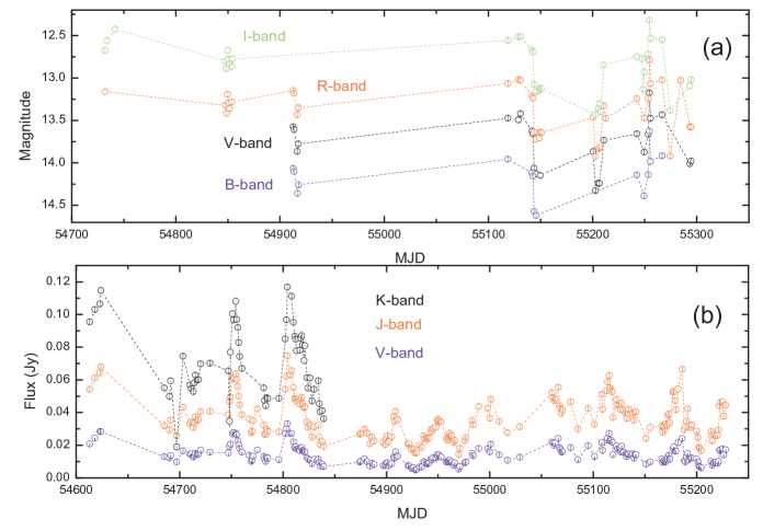
Figure 1: (a) Light curves at I, R, V, and B bands observed by Yunnan Observatories, (b) Light curves at K, J, and V bands of 0716+714 obtained from observations of Kanata telescope at Higashi-Hiroshima observatory (Ikejiri et al. 2011).

where $\delta=(m_{2}-m_{1})_{i}-\overline{m_{2}-m_{1}},~{}\overline{m_{2}-m_{1}}$ is the mean differential magnitude, $N$ is the number of data points in the night. The correction for the interstellar extinction and the color excess were adopted according to Schlegel et al. (1998). Optical photometric data were converted from magnitude system to flux in Jansky (Bessell 2005). The results are plotted in Figure 1a.

3.2 Complementary Optical and other observations from the literatures

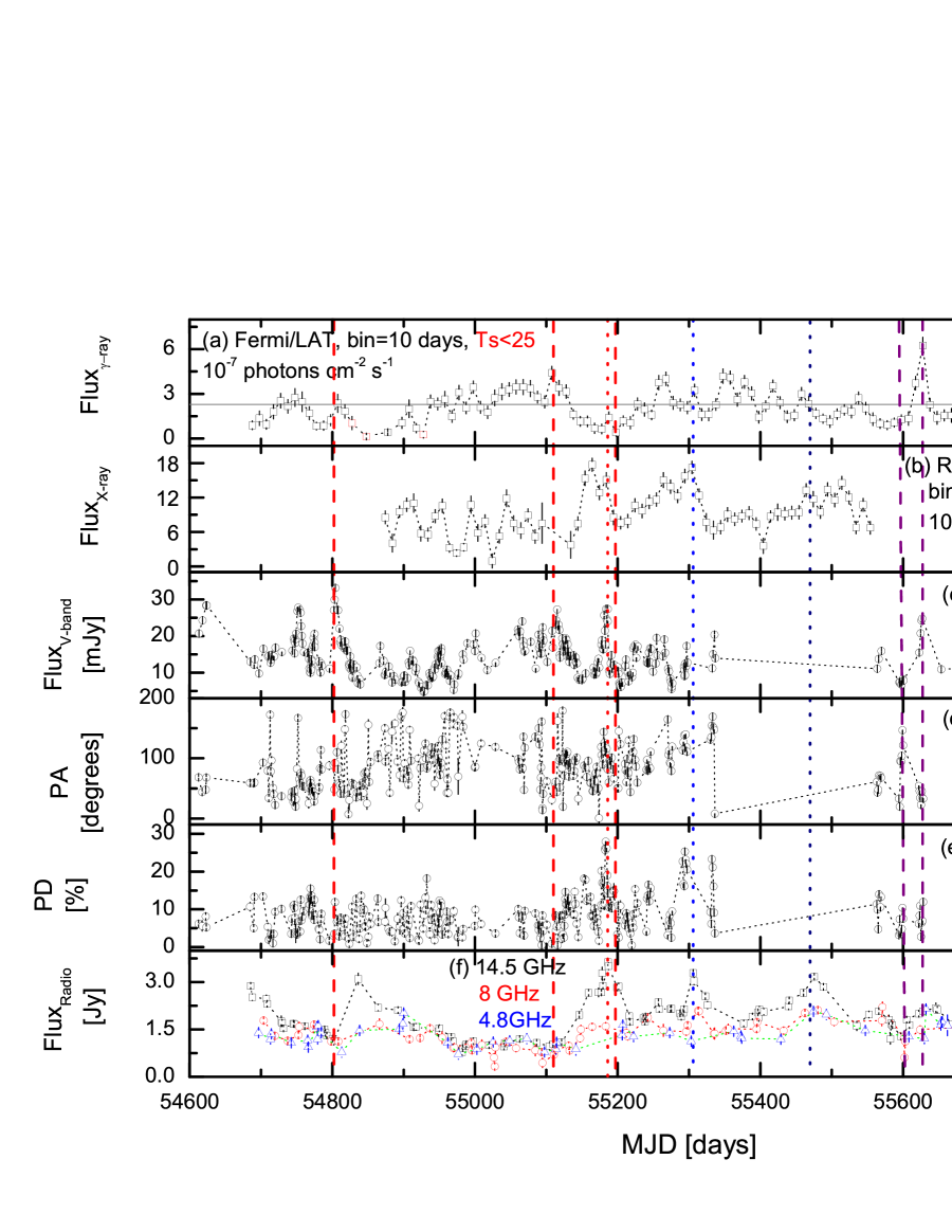
Figure 2: Light curves of radio (UMRAO), optical (detailed data origin can be seen at section 3), X-ray (RXTE/PCA), and $\gamma$-ray (Fermi/LAT) emissions. The horizontal line in plot (a) denotes the average of $\gamma$-ray flux. The four red vertical lines correspond to the four simultaneous SEDs in the text. The two dashed vertical violet lines at 55595 and 55625 MJD indicate the coincidence of a $\gamma$-ray flare with a dramatic change of optical polarization angle. This coincidence is zoomed in to Figure 5. The three dotted vertical lines indicate the peaks of the 14.5 GHz outbursts I, II, and III, which have three well correlated X-ray flares.

Due to the observing time allocation, our photometric data are sparse. In order to match the data-sampling of light curves at X-ray and $\gamma$-ray energies, we collected V band photometric data of S5 0716+714 observed at the 1.5 m Kanata telescope of Higashi-Hiroshima observatory in Japan (Ikejiri et al. 2011) and the 2.3 m Bok telescope and 1.54 m Kuiper telescope at Steward observatory of university of Arizona (Smith et al. 2009) which were also adopted in Rani et al. (2013a), and from two published papers (Poon et al. 2010; Chandra et al. 2011). The V band light curve (Figure 2c) thus contain 324 data points, extending from 54613.0 to 55822.0 MJD.

As mentioned in the Instruction Section, blazars are characterized by their polarized continuum emissions. High linear polarization from radio through optical wavelengths are common in blazars, and usually the fractional variations in polarized flux density are substantially larger than those in total flux density, suggesting that polarization observation is an effective tool for investigating emission process in blazar jets. Variability of polarization in S5 0716+714 was monitored using the Kanata 1.5-m telescope of Higashi-Hiroshima observatory from 2008 to 2009 (Ikejiri et al. 2009), and at the 2.3 m Bok telescope and 1.54 m Kuiper telescope of Steward Observatory of the University of Arizona since 2008 (Smith et al. 2009). The optical polarization, flux, and spectral data of Steward Observatory are publicly presented at their website, and those of Higashi-Hiroshima observatory have been published (Ikejiri et al. 2011). These polarization data were collected. The light curves of the V band PA and polarization degree (PD) data are presented in Figure 2d and 2e, respectively.

The synchrotron peak of S5 0716+714 shifts from time to time in the near-infrared (NIR) and optical bands during different luminosity states. The J and K bands photometric data of S5 0716+714 observed at Higashi-Hiroshima observatory (Ikejiri et al. 2011) were also included in this work. The K-band light curve is from 54613.0 to 54839.2 MJD, and J band light curve is from 54613.0 to 55228.0 MJD. The simultaneous light curves of the V, J, and K bands obtained by the Kanata telescope are presented in Figure 1b.

The radio data were taken from the observations of 26 m paraboloid of the University of Michigan Radio Astronomy Observatory (UMRAO) (Aller et al. 1985, 1999). The light curves at 4.8 GHz, 8 GHz, and 14.5 GHz are from 54685.6 to 55917.2 MJD (Figure 2f). These UMRAO multi-bands data from 54686 to 55600 MJD have been adopted in Rani et al. (2013a).

3.3 X-ray Data Deduction

X-ray data from Proportional Counter Array (PCA) in RXTE and X-ray Telescope (XRT) in Swift are accessible. The PCA observations are more continual than the XRT observations, especially for the time range from 2009 to 2010. X-ray light curve was extracted from the PCA data. S5 0716+714 is too faint to obtain a detailed X-ray spectrum from PCA data whose energy range is 2.6-50 keV which is beyond the spectral concave point of about 3 keV. X-ray spectra were extracted from XRT data with energy range of 0.3-10 keV. The X-ray data were reduced by the FTOOLS software package version 6.9.

3.3.1 RXTE/PCA

We analyzed RXTE observations taken between 2009 February 7 and 2010 December 28. We downloaded the Standard2 data from all layers of PCU2, that operated during all the observations. The data were filtered with the standard criteria: the Earth-limb elevation angle larger than $10\arcdeg$ and the spacecraft pointing offset less than $0.02\arcdeg$. The background files were created by using the program pcabackest and the latest faint source background model since the source intensity $<$ 40 counts/s/PCU (Weng & Zhang 2011). We applied the power law model to fit the RXTE/PCA spectra over the energy range of 2.6-50.0 keV. An interstellar absorption component with the neutral hydrogen column density fixed to the Galactic value ($3.05\times 10^{20}$ ${\rm cm^{-2}}$, Murphy et al. 1996) was also included. The unabsorbed flux and its error were also calculated in the 2.6-50.0 keV with the cflux in XSPEC. The ten days bin X-ray light curve is represented in Figure 2b.

3.3.2 Swift/XRT

The initial event cleaning was performed using the xrtpipeline script, with the standard quality cuts (Weng & Zhang 2011). The source spectra were extracted with xselect, from circles with radius of 20 pixels centered at the nominal position of S5 0716+714, while the background spectra were taken from a annulus regions with radius 30 and 60 pixels. If data were suffered from pileup, the annular regions were used to describe the source, and the excluded region radius depended on the current count rate . We also produced the ancillary response file with xrtmkarf to facilitate subsequent spectral analysis. The response files (v013) were taken from the CALDB database. Finally, the spectra were grouped to require at least 20 counts per bin to ensure valid result using $\chi^{2}$ statical analysis. The XRT spectra are exhibited in Table 1.

3.4 Fermi/LAT Data Reduction

The Pass 7 $\gamma$-ray data were downloaded from LAT data server, with time range from 4th August 2008 to 22th November 2011. The LAT event photons from 0.1 to 300 GeV were selected. The LAT data analysis was performed with instrument response functions of P7SOURCE_V6, using the updated standard ScienceTools software package version v9r23p1. For the LAT background files, we used gal$\_$2yearp7v6$\_$v0.fits as the galactic diffuse model and iso$\_$p7v6source.txt for the isotropic spectral template. For data preparation, evclass=2 was adopted for gtselect. The maximum zenith angle was set to $100\arcdeg$. We used unbinned likelihood algorithm (Mattox et al. 1996) implemented in the gtlike task to extract the flux and spectra. LogParabola function was used as the spectral model. All sources from the Second Fermi/LAT catalog (2FGL, Nolan et al. 2012) within $15\arcdeg$ of the source position were included. The flux and spectral parameters of sources within $10\arcdeg$ “region of interest” (ROI) were set free, while parameters of sources that fell outside the ROI were freezed at the 2FGL values.

For light curves, fit of each bin was scrutinized to make sure that the fit quality is satisfactory and there is no background source with negative TS value and exotic parameter. In a few low TS cases, when the LogParabola function was not applicable, single power-law model was used instead. There are only three fits with TS values lower than 25 in the $\gamma$-ray light curve analysis and the lowest TS value is 17 ($\geq 4\sigma$). We did not set them as upper limits. The ten days bin $\gamma$-ray light curve is shown in Figure 2a. The python script named SED$\_$scripts$\_$v13.1 from $Fermi$ User Contributions was used to obtain $\gamma$-ray spectra. In the spectral analysis, when the TS value was lower than 25, flux was replaced by 2$\sigma$ upper limit. All errors reported in the figures or quoted in the text for $\gamma$-ray are 1$\sigma$ statistical errors. The estimated relative systematic uncertainties on the flux and effective area, are set to $10\%$ at 100MeV, $5\%$ at 500MeV and $20\%$ at 10GeV (Abdo et al. 2010b).

4 THE VARIABILITY PROPERTIES

4.1 Spectral and Flux Variability around SED Peaks

4.1.1 Spectral Variability in the NIR-Optical Bands

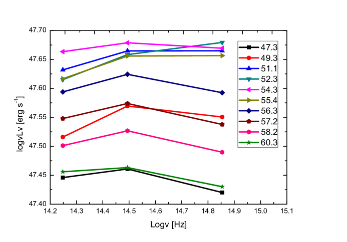
Figure 3: NIR-optical SEDs, constructed with simultaneous V, J, K data observed from Kanata telescope (Ikejiri et al. 2011). These data have been already corrected for the interstellar extinction and the color excess. The numbers represent the corresponding dates of the SEDs, MJD-54700.

The peak frequencies and their changes of blazar SED are important to obtain the parameters of emission model. The SEDs from NIR to optical of S5 0716+714 are obtained from simultaneous V, J, and K bands photometric data around the maximum flux at 54754.3 MJD when the flux variation is intense and the time covering of the observations is good (see Figure 3). The data observed at 54748.3 MJD are abandoned for the large error and peculiarly low flux in K band. The SEDs are characterized by the inversions around J band in relatively low condition, which suggests that the synchrotron peak is likely close to the J band at the observational frame. When the source flares, SEDs become flat between J and V bands. The SED is not inverted at 54752.3 MJD, which means the frequency of the synchrotron peak is higher than V band. Similar bluer-when-brighter behavior has been found by Villata et al. (2008) from contemporaneous GASP-WEBT to Swift/UVOT data for S5 0716+714.

4.1.2 Spectral Variability at $\gamma$-rays

The fit for 40 months LAT data is accomplished and the result gives

$$\frac{dN}{dE}=(1.27\pm 0.02)\times 10^{-10}(\frac{E}{\rm 428.66MeV})^{-((2.03\pm 0.02)+(0.03\pm 0.007)log(\frac{E}{\rm 428.66MeV}))},$$ (2)

with the average flux of (22.8 $\pm$ 0.4)$\times 10^{-8}$ ph $\rm cm^{-2}s^{-1}$ which is similar to the EGRET detection of (2.0 $\pm$ 0.4) $\times 10^{-7}$ ph $\rm cm^{-2}s^{-1}$ (Lin et al. 1995). The 40 months LAT data is fitted by 20 energy bins. The average spectrum departs from power law over 99% confidence tested by the spectral curvature index $\mathcal{C}$ (Abdo et al. 2010b). A broken power law also gives an acceptance to the spectrum, including a flat component between 0.1 and 1 GeV ($\Gamma=2.033\pm 0.004$) and a descent one up to higher energy ($\Gamma=2.282\pm 0.023$). The index of the decent part is in accordance with the non-simultaneous TeV deabsorbed photon index of 1.8$\pm$0.6 (Anderhub et al. 2009). The highest energy photon event with the probability of 0.9998 by gtsrcprob is 207.4 GeV. It is much higher than 70 GeV for BL Lacertae during the first 18-month period (Abdo et al. 2011).

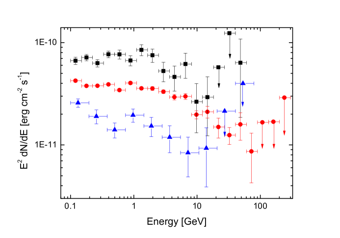
Figure 4: $\gamma$-ray spectra in different states. The black squares represent the spectrum corresponding to the strongest flare at 55857.7 MJD. The red circles represent the average spectrum. The blue triangles correspond to the low state spectrum.

Simultaneous $\gamma$-ray spectra are used to study the $\gamma$-ray spectral variability of the source. Spectra of five strongest $\gamma$-ray flares which peak at 54807.7, 55107.7, 55627.7, 55757.7 and 55857.7 MJD, correspond to the flaring state. Another spectrum is obtained using $\gamma$-ray data from 55147.7 to 55207.7 MJD when the flux is in the low state. In the energy range from 0.1 GeV to 1 GeV, the flaring state spectra are flat or even ascending, which are harder than the low state spectrum. Spectral variability around the second SED bump is similar with it around the first SED bump. The general trend that when flux raises the peaks of the SED bumps become bluer is the classical behavior of SED evolution of blazars (Ulrich et al. 1997). The low state spectrum and a flaring state spectrum corresponding to the strongest flare, together with the average spectrum, are shown in Figure 4.

4.1.3 The Shortest Variability Timescale at $\gamma$-rays

S5 0716+714 underwent three strong $\gamma$-ray flares in 2011. Their peak fluxes are almost three times as the average flux. The highest daily flux is $(1.69\pm 0.25)\times 10^{-6}$ ph $\rm cm^{-2}s^{-1}$ at 55854.2 MJD which is lower than the AGILE detection of $(2.03\pm 0.75)\times 10^{-6}$ ph $\rm cm^{-2}s^{-1}$ (Chen et al. 2008). The most intense variation appears when the flux increases from $(3.74\pm 1.67)\times 10^{-7}$ ph $\rm cm^{-2}s^{-1}$ at 55853.2 MJD to $(1.69\pm 0.25)\times 10^{-6}$ ph $\rm cm^{-2}s^{-1}$ at 55854.2 MJD. The $\gamma$-ray flux varies roughly 4.5 times at the interday timescale, which is more violent than a flux increase by a factor of four in three days (Chen et al. 2008). The doubling time less than one day in this flare agrees on the finding of Rani et al. (2013b). Such a rapid $\gamma$-ray variation allows us to make a constraint on Doppler factor avoiding the heavy absorption from $\gamma\gamma$ process (Begelman et al. 2008). The doubling time is about 21 hours and the highest energy bin in the average $\gamma$-ray spectrum with $\rm TS\geq 25$ centers at about 72 GeV. Using the equation in Dondi $\&$ Ghisellini (1995), $\delta\geq 7.5$. Rani et al. (2013b) uses the highest photon of 207.4 GeV as the absorbed photon and makes the constraint of $\delta\geq 9.1$.

4.2 Multi-wavelength Correlations

4.2.1 Correlations of Radio/X-ray and Optical/$\gamma$-ray Variations

The PCA X-ray and 14.5 GHz light curves seem to be well correlated. Three flares of 14.5 GHz band at 55186.2, 55305.9 and 55475.5 MJD respectively correspond to the X-ray flares at 55185.6, 55302.8 and 55464.5 MJD (see three dotted vertical lines in Figure 2). The low states between these flares in both energy bands are also corresponding. However, the outlines of 14.5 GHz flares are probably broader than those in the X-rays. No obvious correlation can be directly seen between other two radio bands and the PCA X-ray light curves. The flaring behaviors seem to be washed out at 4.8 and 8 GHz.

Searching the existence of the correlation between optical and $\gamma$-ray variations had been performed for S5 0716+714 since the CGRO era (Ghisellini et al. 1997). Although the optical data in our work is limited, most optical flares have the corresponding $\gamma$-ray ones. The optical flux raises quickly during the ascent phase of the strong $\gamma$-ray flare at 55627.7 MJD (see the violet vertical line in Figure 2). Even in the extreme low state of $\gamma$-ray, there probably exists a $\gamma$-ray flare corresponding to a strong optical flare. On the other side, three strongest optical flares with nearly constant optical peak fluxes, correspond to three $\gamma$-ray flares with their $\gamma$-ray peak fluxes changing three times. A $\gamma$-ray flare at 54807.7 MJD with the peak flux of $(2.36\pm 0.61)\times 10^{-7}$ ph $\rm cm^{-2}s^{-1}$ just above the average flux, corresponds to the strongest optical flare at 54804.3 MJD. One of the strongest $\gamma$-ray flare at 55107.7 MJD when the peak flux is $(4.41\pm 0.45)\times 10^{-7}$ ph $\rm cm^{-2}s^{-1}$, correlates a strong optical flare at 55115.3 MJD. In this case, the $\gamma$-ray peak flux is almost twice as the average flux. During the long low state of $\gamma$-ray from 55132.7 to 55222.7 MJD, another $\gamma$-ray flare at 55187.7 MJD with the peak flux of $(1.42\pm 0.38)\times 10^{-7}$ ph $\rm cm^{-2}s^{-1}$, corresponds to a strong optical flare at 55185.9 MJD. Peak flux of this $\gamma$-ray flare is nearly half of the average flux.

4.2.2 Coincidence of $\gamma$-ray Flux and Optical PA Variation

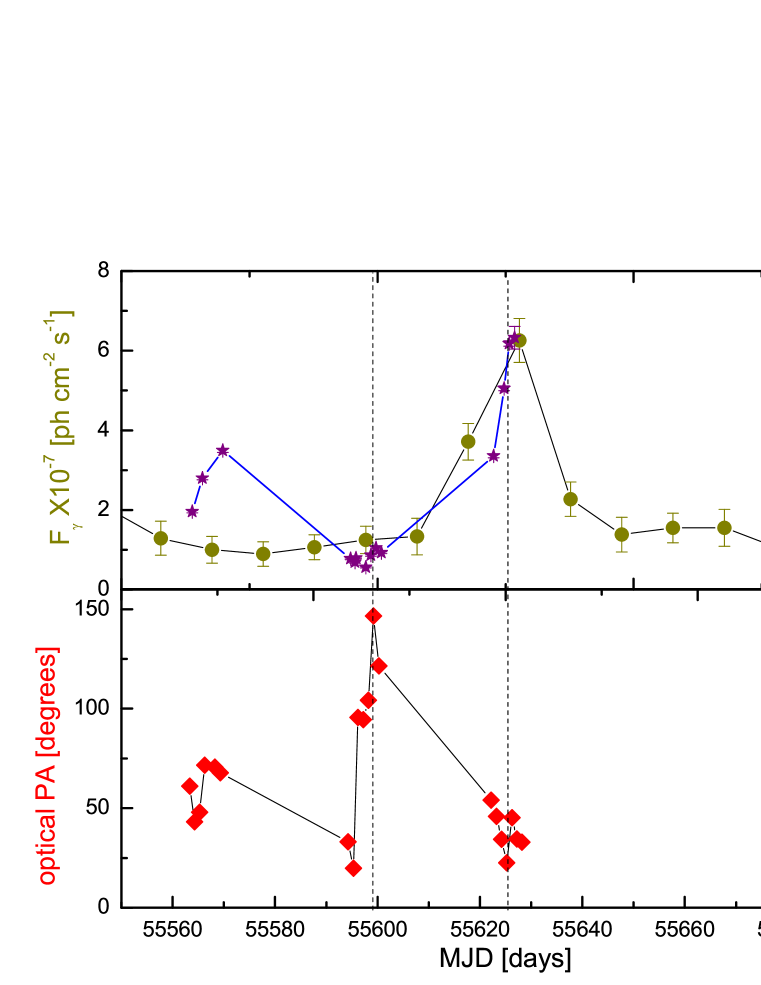
Figure 5: The coincidence of $\gamma$-ray and optical flares with a dramatic change of V band PA. The dark yellow filled circles represent the $\gamma$-ray fluxes, the purple stars are the optical fluxes and the red squares represent the V band PA. Between the two vertical dash lines, the fluxes of the $\gamma$-ray and the optical increase while the PA shows the overall downward trend.

We find the coincidence of a $\gamma$-ray flare with a dramatic change of optical PA at 2011 March (see Figure 5). Within $\sim$ 30 days, the $\gamma$-ray flux sharply increases from the low state at 55597.7 MJD to the flare peak at 55627.7 MJD. The optical PA sharply increases from $(19.9\pm 0.1)\arcdeg$ at 55595.3 MJD to $(146.6\pm 0.1)\arcdeg$ at 55599.2 MJD within 5 days and then decreases to $(22.6\pm 0.2)\arcdeg$ at 55625.2 MJD within 27 days (see two dashed vertical lines in Figure 5). Within the increasing phase of PA, the rotation rate of PA is $25\arcdeg$ per day. Within the decreasing phase of PA, the rotation rate of PA is $4.6\arcdeg$ per day. There is a flare in the V-band flux corresponding to this sharp $\gamma$-ray flare. At the increasing phase of this optical flare, the optical PA has a dramatic change as in the sharp $\gamma$-ray flare (see Figure 5). Larionov et al. (2013) finds that a $180\arcdeg$ rotation of the position angle of the optical linear polarization coincides with strong flares in $\gamma$-ray and optical bands in 2011 October. Actually, these similar observational phenomena have been found in two of the three strong $\gamma$-ray flares in 2011. Larionov et al. (2008) reports another coincidence of a huge optical outburst with a $360\arcdeg$ rotation of optical PA in 2008 April while simultaneous $\gamma$-ray observation is missing. This phenomenon seems to be a common occurrence for the source. A similar behavior has been found in 3C 279 by Abdo et al. (2010e). It is suggested that the sharp $\gamma$-ray flare is correlated with the dramatic change of optical polarization, likely due to a single, coherent event, rather than a superposition of multiple but causally unrelated, shorter duration events. Co-spatiality of optical and $\gamma$-ray emission regions, and a highly ordered jet magnetic field are indicated (Abdo et al. 2010e).

4.2.3 Strong Optical and X-ray Activities at the $\gamma$-ray Low State

An interesting variability phenomenon of S5 0716+714 is that intense variations appear in the X-rays, the optical flux and PD during the long low state of the $\gamma$-rays from 55132.7 to 55222.7 MJD. The highest flux in the X-rays is $(14.47\pm 2.21)\times 10^{-12}$ erg $\rm cm^{-2}s^{-1}$ at 55164.6 MJD, raising from $(5.27\pm 1.94)\times 10^{-12}$ erg $\rm cm^{-2}s^{-1}$ at 55143.2 MJD. There is a strong secondary X-ray flare whose peak flux is $(13.25\pm 1.98)\times 10^{-12}$ erg $\rm cm^{-2}s^{-1}$ at 55185.6 MJD. The flux of X-ray becomes low for $(5.00\pm 1.68)\times 10^{-12}$ erg $\rm cm^{-2}s^{-1}$ at 55213.0 MJD. The fluxes of the optical double peaks are both $27.4\pm 0.3$ mJy at 55183.8 and 55185.9 MJD, with the maximum optical PD of $(25.69\pm 0.80)$% at 55183.3 MJD. The optical flux rises from $8.0\pm 0.1$ mJy at 55149.9 MJD and drops to $6.2\pm 0.03$ mJy at 55204.3 MJD. The lowest optical PD in this epoch is $(1.69\pm 0.69)$% at 55173.7 MJD. There is a flare of 14.5 GHz peaks at 55186.2 MJD. However, the duration of this radio flare is longer than flares in other bands. A $\gamma$-ray flare with peak flux of $(1.41\pm 0.38)\times 10^{-7}$ ph $\rm cm^{-2}s^{-1}$ at 55187.7 MJD corresponds to the optical, optical PD and the secondary X-ray flares. The peak flux of this $\gamma$-ray flare is lower than the averaged flux while the corresponding peak fluxes in other bands maintain in high state. But it is nearly twice as the flux at 55177.7 MJD of (0.63$\pm 0.32)\times 10^{-7}$ ph $\rm cm^{-2}s^{-1}$ and roughly 3.6 times as the flux at 55197.7 MJD of (0.39$\pm 0.25)\times 10^{-7}$ ph $\rm cm^{-2}s^{-1}$. So the $\gamma$-ray variability amplitude is comparable with other bands. During this $\gamma$-ray low state epoch, the TS value for each bin is larger than 25, which makes the variability amplitude reliable. The fluxes of X-rays and $\gamma$-rays all vary nearly three times. The intrinsic variability amplitudes of these bands could be higher due to their ten days averaged fluxes. The flux of optical V band varies more than four times. The most violent behavior is shown as over ten times variation on the optical PD. The X-ray flare at 55143.2 MJD, which leads the optical and $\gamma$-ray flares, is probably orphan discussed in Rani et al. (2013a).

Similar work using data from Swift and AGILE satellites has been performed (Giommi et al. 2008). The multi-wavelength observational results are similar to ours. However, it is claimed that the highly variable optical and soft X-ray fluxes accompany with a constant $\gamma$-ray flux which is based on the AGILE observation with low counting statistics. Corresponding $\gamma$-ray flare may be missed.

4.3 Statistic Analysis on Multi-wavelength Light Curves

4.3.1 Time Lags

The discrete correlation function (DCF; Edelson & Krolik 1988) is a technique in time series analysis for finding time lags between different light curves utilizing a binning scheme to approximate the missing data. The z-transformed discrete correlation function (ZDCF; Alexander 1997) can estimate the cross-correlation function in the case of non-uniformly sampled light curves. The ZDCF is a binning type of method as an improvement of the DCF technique, with a notable feature that the data are binned by equal population rather than equal bin width $\Delta\tau$ as in the DCF. These light curves at the radio, infrared, optical, and X-ray bands are sampled sparsely and unequally for S5 0716+714. Thus, as in the previous researches on the unequally sampled light curves (Liu et al. 2008, 2011a, b), time lags will be analyzed by the ZDCF. From these ZDCF profile bumps closer to the zero-lag, the centroid time lags $\tau_{\rm{cent}}$ which are used as the estimation of time lag, are computed using all points with correlation coefficients $r\geq 0.8r_{\rm{max}}$.

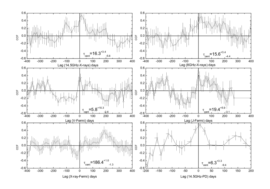
Figure 6: ZDCFs between $\gamma$-rays, X-rays, V band, J band, 14.5 GHz and 8 GHz emissions, together with V band PD. Considering the bin sizes of the PCA X-ray and LAT $\gamma$-ray light curves, radio/hard X-ray and the optical/$\gamma$-ray variations are suggested to be correlated with zero-lag

The calculated ZDCFs are presented in Figures 6 for the light curves in Figures 1 and 2. Considering the bin sizes of the X-ray and $\gamma$-ray light curves, 14.5GHz/X-ray and the optical V band/$\gamma$-ray variations appear to be zero-lag. The J-band light curve (Figure 1), which is well sampled with shorter time range than the V band light curve, also seems to zero-lag the $\gamma$-ray light curve. We also use the classic DCF method to check our correlation results. In general, the correlation results from ZDCF and DCF are in agreement. The 14.5GHz/X-ray, the V band/$\gamma$-ray and X-ray/$\gamma$-ray variations are all strongly correlated with over 99.9% confidence level. Rani et al (2013a) and Larionov et al. (2013) also suggest the optical V band/$\gamma$-ray variations are correlated with zero-lag. However, we find that the relationship between the 14.5 GHz and the $\gamma$-ray emissions is likely not tight. The correlation coefficient is relatively low and the lag is not stable for different bin sizes. Rani et al (2013a) finds that the confidence levels of the correlations of $\gamma$-ray/37 GHz and $\gamma$-ray/230 GHz are lower than 3$\sigma$.

4.3.2 Fractional Variability Amplitude

In order to estimate the total variability of each light curve, we use the RMS fractional variability amplitude $F_{\rm{var}}$ (e.g., Edelson et al. 2002; Vaughan et al. 2003). The fractional variability amplitude $F_{\rm{var}}$ is defined as

$$F_{\rm{var}}=\sqrt{\frac{S^{2}-<\sigma^{2}_{\rm{err}}>}{<F>^{2}}},$$ (3)

where $<F>$ is the mean flux for the N points in the light curve, $S^{2}$ denotes the total variance of the light curve, and $<\sigma^{2}_{\rm{err}}>$ denotes the measured mean square error of the data points:

$$S^{2}=\frac{1}{N-1}\sum^{\rm{N}}_{\rm{i=1}}(F_{\rm{i}}-<F>)^{2},$$ (4)

$$<\sigma^{2}_{\rm{err}}>=\frac{1}{N}\sum^{\rm{N}}_{\rm{i=1}}\sigma^{2}_{\rm{err,i}}.$$ (5)

The error on $F_{\rm{var}}$ is (Edelson et al. 2002)

$$\sigma_{F_{\rm{var}}}=\frac{1}{F_{\rm{var}}}\sqrt{\frac{1}{2N}}\frac{S^{2}}{<F>^{2}}.$$ (6)

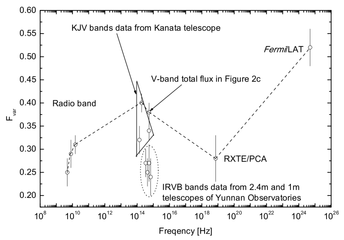
Figure 7: Fractional variability amplitude as function of frequency. The dashed line shows the data in Table 2.

For light curves in Figure 2 and the J band light curve in Figure 1, the calculated results of $F_{\rm{var}}$ are listed in Table 2. For all the light curves in Figures 1 and 2, the calculated $F_{\rm{var}}$ are presented in Figure 7. The fractional variability amplitude violently varies with the frequency. Firstly, $F_{\rm{var}}$ increases with increasing frequency within the radio band. This trend is same as that found in 3C 273 (e.g., Soldi et al. 2008). Secondly, $F_{\rm{var}}$ increases from the radio to J band, decreases to V band and X-rays, and then increases to $\gamma$-ray band (see Figure 7). Variability in the $\gamma$-ray band is the most violent. The sampling rates and time intervals of light curves significantly influence $F_{\rm{var}}$, and this is clearly shown in the light curves at the K, J, I, R, V, and B bands (see Figure 7).

4.3.3 Characteristic Variability Timescale

The zero-crossing time of the autocorrelation function (ACF) of a light curve was defined as a single characteristic variability timescale (Giveon et al. 1999). It is a well-defined quantity and used as a characteristic variability timescale (e.g., Alexander 1997; Giveon et al. 1999; Netzer et al. 1996). Comparison of widths of the ACF between different bands can shed light on the relation between the mechanism and location of emission in these wave bands (Chatterjee et al. 2012). Another function used in variability studies to estimate the variability timescale is the first-order structure function (SF; e.g., Trevese et al. 1994). There is a simple relation between the ACF and the SF (see eq. [8] in Giveon et al. 1999). Therefore, only an ACF analysis is performed on our light curves. The ACF is estimated by the ZDCF (Alexander 1997). Following Giveon et al. (1999), a fifth-order polynomial least-squares procedure is used to fit the ZDCF, and this fifth-order polynomial fit is used to evaluate the zero-crossing time.

Calculated ACFs are presented in Figure 8 for the light curves in Figure 2. These characteristic variability timescales of S5 0716+714 at the 14.5 GHz, V, X-ray, and $\gamma$-ray bands are comparable to each other, $\sim$ 60–90 days. We also check the effect of the binning on our results. Changing of bin size can not significantly influence our tendency. These comparable characteristic variability timescales indicate that these emission variations likely have the same origin. While the origin of 14.5 GHz emission could be complicated. Since the 14.5 GHz emission is well correlated with the hard X-rays and the light curve of 14.5 GHz seems to be less rapidly variable than other three bands, the 14.5 GHz emission is probably consisted of two different components. One component could be more relative with the high energy emissions and from the compact radiation region. The other component is from a extended region and less rapidly variable. The characteristic variability timescale of 14.5 GHz from our ACF analysis likely corresponds to the first component. Rani et al. (2013b) uses the SF analysis to obtain the $\gamma$-ray variability timescale of $\sim$75 days. Rani et al. (2013a) finds that the variability timescales of radio bands from 15 GHz to 230 GHz are in the range of $\sim$ 60–90 days by the SF analysis. The variability timescale of the V band light curve is suggested to be $\sim$60 days by Lomb-Scargle periodogram analysis (Rani et al. 2013a). Our ACF results agree on these similar variability timescale studies for S5 0716+714.

4.4 Implication of Multi-wavelength Variability

Concave X-ray spectra (Table 1) with the break energies of $\sim$3 keV based on our XRT data analysis agree with the results from literatures. The hard X-ray component is considered to be from the IC process by the low energy electrons in the leptonic models (Giommi et al. 1999; Tagliaferri et al. 2003; Zhang 2010). Our X-ray light curve is obtained from the PCA data with energy range of 2.6-50 keV. The radio emission of blazars is widely accepted from the synchrotron process by the low energy electrons. If the radio and the hard X-ray emissions both come from the low energy electrons, 14.5 GHz and the PCA X-ray light curves should be correlated. Such a prediction is confirmed by our correlation analysis, strongly supporting the leptonic models.

Correlation with a zero-lag between the optical V band and $\gamma$-ray variations is also found, which agrees on similar works (Rani et al 2013a; Larionov et al. 2013). 3C 66A, with the source type similar to S5 0716+714, shows a clear correlation between GeV $\gamma$-ray and optical R band with a time lag of $\lesssim$ 5 days (Reyes et al. 2011). Well correlations between optical/IR and $\gamma$-rays in six blazars have been found with zero-lags for FSRQs (Bonning et al. 2012). There are $\gamma$-ray and optical flares at about 55183 MJD when a flare of optical PD coincides. The coincidence of $\gamma$-ray and optical flares with a dramatic change of optical PA at 2011 March is found. Similar behavior happens at 2011 October (Larionov et al. 2013). All the above observations suggest a tight relationship between the optical and the $\gamma$-ray emissions. These multi-wavelength variation phenomena accord with the leptonic models.

In view of the global frequency range, the variability amplitudes and characteristic variability times of S5 0716+714 from radio to $\gamma$-rays can be naturally explained by the leptonic models. We find that the $F_{\rm{var}}$ is a function of frequency. The $F_{\rm{var}}$ increases from the radio band to optical band, decreases to hard X-rays, and then increases to $\gamma$-rays. In the leptonic models, the electrons which generate the optical and $\gamma$-ray emissions have higher energies than those for radio and hard X-ray emissions. The radiation cooling time of the high energy electrons is shorter than it of the low energy electrons. Through our ACF analysis, the characteristic variability times of 14.5 GHz, V band, X-ray and $\gamma$-ray are comparable to each other, which agrees on the variability timescales from SF analysis (Rani et al. 2013a,b). It is indicated that variations of these emissions likely have the same origin. These four bands emission are suggested to be from the same population of electrons in the leptonic models. Although the variation origin of blazars is extremely complicated, the variation of the properties of the electrons can be one of the most important reasons for variability of emissions of these four energies.

“orphan” $\gamma$-ray flare is not found by comparing the optical light curve. Considering the strong correlation with a zero lag between optical and $\gamma$-ray flux variations and coincidences of $\gamma$-ray and optical polarization variations, the hadronic models do not have the same nature explanation for these observations than the leptonic models.

5 SED MODELING

The SED modeling is a powerful tool to test different radiation models for blazars. In this paper, a homogeneous one zone synchrotron plus IC model is used to calculate the jet emission of S5 0716+714. The broadband electromagnetic emission comes from a compact homogeneous blob with relativistic speed having the radius of $R$ embedded in the magnetic field. A broken power law spectrum for particle distribution has been assumed,

$$N(\gamma)=\left\{\begin{array}[]{ll}K\gamma^{-p_{1}}&\mbox{ $\gamma_{\rm min}\leq\gamma\leq\gamma_{br}$}\\ K\gamma_{\rm br}^{p_{2}-p_{1}}\gamma^{-p_{2}}&\mbox{ $\gamma_{\rm br}<\gamma\leq\gamma_{\rm max}$.}\end{array}\right.$$ (7)

Such a broken power law distribution can be the result of the balance from the particle cooling and escape in the blob. The parameters of this model include, the radius $R$ of the blob, the magnetic field strength $B$, electron break energy $\gamma_{\rm br}$, the minimum and maximum energy $\gamma_{\rm min}$, $\gamma_{\rm max}$, of the electrons, the normalization of the particle number density $K$, and the indexes $p_{1,2}$ of the broken power law particle distribution. The frequency and luminosity can be transformed from the jet frame to observational frame as: $\nu=\delta\nu^{\prime}/(1+z)$ and $\nu L_{\nu}=\delta^{4}\nu^{\prime}L_{\nu^{\prime}}^{\prime}$, where the Doppler factor $\delta=1/\left[\Gamma\left(1-\beta\cos\theta\right)\right]$. The synchrotron self-absorption and the Klein-Nishina effect in the IC scattering are properly considered in our calculations. The detailed constraints of the SED modeling can be found in Tavecchio et al. (1998) and Sikora et al. (2009).

We use the $\chi^{2}$-minimization method to obtain the best fitting input parameters. We make special constraints on parameters of B and $\delta$. The values of these parameters are varied in wide ranges to calculate the corresponding values of $\chi^{2}$. Then, we obtain the probability of the fit by $p\propto e^{-\chi^{2}/2}$. We plot the contours of p in the B-$\delta$ plane and constrain the value of the B and $\delta$ at 1$\sigma$ level. Detailed SED modeling strategy can be found in Zhang et al. (2012).

5.1 Average SED modeling

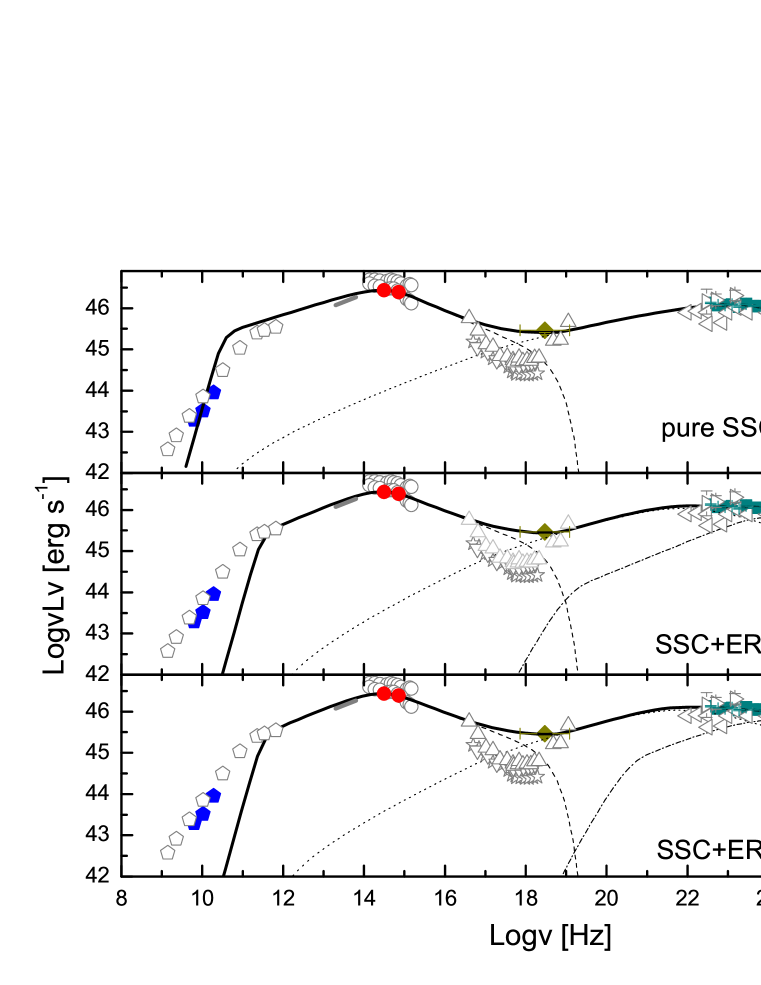
Figure 9: Modeling the average SED with different models. Filled symbols are from our work and hollow symbols are collected from the literatures (radio, Fuhrmann et al. 2008; IR/optical, Chen $\&$ Shan 2011, Villata et al 2008; X-ray, Tagliaferri et al. 2003; $\gamma$-ray, Tagliaferri et al. 2003, Giommi et al. 2008). Blue pentagons are the averaged fluxes of 4.8, 8, 14.5 GHz from UMRAO. Red filled circles are the J and V band optical average fluxes. Yellow diamond is the average X-ray flux for 3-50 keV from RXTE/PCA. Cyan squares represent the 40 months average $\gamma$-ray spectrum from Fermi/LAT. The dash line represents the calculated synchrotron emission, the dot line corresponds to the SSC component and the dash dot line is the ERC part.

Thanks to the long accumulative observation time, the average $\gamma$-ray spectrum from 0.1 GeV to almost 100 GeV with relatively small error brings much more information than observations before, the EGRET and AGILE observations (Lin et al. 1995; Chen et al. 2008). Modeling the average SED with different models are shown in Figure 9 and the input parameters are listed in Table 3.

S5 0716+714 possesses violent variations across its broadband electromagnetic radiation. It is a famous IDV source in the radio and optical bands, doubling time of 7000 s at X-ray, and $\gamma$-ray flux changing 4.5 times for two days, which are strict constraints on the emission region, $R\leq$ c$t_{var}\delta(1+z)^{-1}$ (Begelman et al. 2008). The Doppler factor can be constrained by rapid variations ($\gtrsim$ 5-15, Fuhrmann et al. 2008) and kinematic study ($\approx$ 20-30, Bach et al. 2005). The strength of the magnetic field can be constrained by the inverted radio spectra demonstrated as the result of synchrotron self-absorption ($\gtrsim$ 0.07-0.11 $\delta$G, Fuhrmann et al. 2008)

In Table 3, it can be seen that for pure SSC model which is usually successful for TeV blazars, the input model parameters are extreme. When the variability timescale is set to one day, the Doppler factor value becomes extraordinarily large which conflicts with the typical value from kinematic studies for blazars. The Doppler factor is reduced to $39.6_{-3.1}^{+3.8}$ when variability timescale is set to ten days. However, the variability timescale of ten days disagrees on the observations of fast variability from the radio to $\gamma$-rays. Meanwhile, the magnetic field B is $0.006_{-0.002}^{+0.001}$ Gause which is not harmonious with the typical value from similar SED fitting works before (eg. Tagliaferri et al. 2003; Giommi et al. 2008). The large frequency ratio of the SSC peak to synchrotron peak may bring out these abnormal parameters. The pure SSC model is also not favorable due to its failure for explaining the extreme fast optical variability (Danforth et al. 2013).

Although no thermal components have been detected from spectroscopic observations (Chen & Shan 2011; Shaw et al 2009; Danforth et al. 2013), scattering of weak external emissions could possibly contribute the $\gamma$-ray emission of the source. Because the synchrotron peak of S5 0716+714 locates at NIR/optical band at the observation frame, the hot dust emission can be heavily diluted by the strong nothermal continuum. A prominent infrared excess indicative of dust emission with 1200 K in 4C 21.35 has been detected, which proves the hot dust emission can be the main contribution to the external seed photons for IC process (Malmrose et al. 2011). Both the assumed hot dust and BLR emissions are individually considered in the average SED modeling. The hot dust and BLR emissions are approximated as black body emissions of the temperature of 1200 K and peaking at the frequency of the Ly$\alpha$ line, respectively. For each fitting process, the variability timescale is set to one day and the photon energy density is set free.

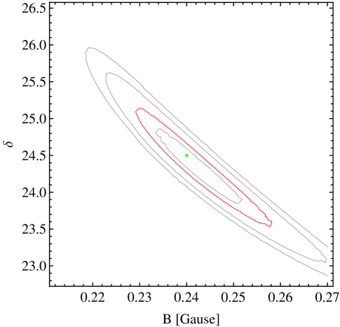
Figure 10: The contours of the p in the B-$\delta$ plane, while $p\propto e^{-\chi^{2}/2}$. Four contours correspond to the p of 0.05, 0.1, 0.2 and 0.26, respectively. And the contour of p=0.2 is drawn as red color, which corresponds to the 1$\sigma$ level of the Gaussian fit for the B-p and $\delta$-P distribution. The green spot demonstrates the location of the best fit.

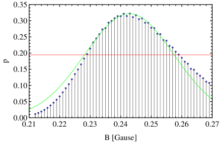
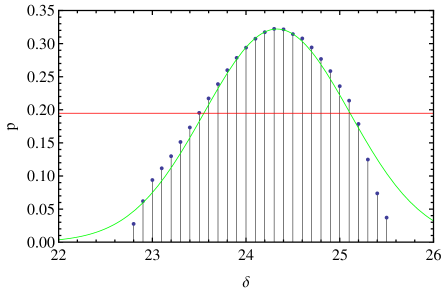
Figure 11: The distributions of p with different values of B and $\delta$. The green lines are the Gaussian fits. The red horizontal lines are obtained from the 1$\sigma$ level of the Gaussian fits with the p value of 0.195. The 1$\sigma$ uncertainties of the B and $\delta$ are obtained from the intersections between the B-p and $\delta$-p distributions and the red horizontal lines.

The contours of p for the case of SSC+ERC model with the hot dust photons are shown in Figure 10. The B and $\delta$ distributions of p can be seen in Figure 11. The values of $\delta$ are $24.5^{+0.6}_{-0.7}$ and $23.3^{+0.7}_{-0.9}$ corresponding to the hot dust and BLR emissions as the external seed photons, respectively. These values are more agreeable on the observations than the $\delta$ value from the pure SSC model with variability timescale as one day. The magnetic field intensity values are $0.24^{+0.02}_{-0.01}$ and $0.28^{+0.02}_{-0.02}$ corresponding to the hot dust and BLR emissions as the external seed photons, respectively. Although these values are still lower than the constraint from radio spectra (Fuhrmann et al. 2008), they are more reasonable than the magnetic field intensity from the pure SSC model. The SSC+ERC models are more favorable avoiding the extreme input parameters and better explaining the fast variability than the pure SSC model.

5.2 Simultaneous SED modeling

As mentioned in Section 4.2, three strong optical flares with nearly constant optical peak fluxes correspond three $\gamma$-ray flares with their $\gamma$-ray peak fluxes changing three times. At 55187.7 MJD, peak flux of the $\gamma$-ray flare is even lower than the average flux while peak fluxes of corresponding flares in optical and X-ray bands maintain in high state. This seems to be abnormal for the leptonic models.

Three simultaneous SEDs are obtained for optical and $\gamma$-ray flaring state, together with another simultaneous SED for multi-wavelength low state. For the first SED, the strongest optical flare at 54804.3 MJD corresponding to a $\gamma$-ray flare at 54807.7 MJD with peak flux just above the average flux is focused. No simultaneous X-ray observation is found. The second SED corresponds to one of the strongest $\gamma$-ray flare at 55107.7 MJD correlated with a strong optical flare at 55115.3 MJD. X-ray constraint is the interpolation of the edges of the PCA observation blank at 55091.0 and 55136.0 MJD. Violent X-ray and optical activities have been detected during the long low $\gamma$-ray period from 55132.7 to 55222.7 MJD. Two SEDs are corresponding to the low and high states for highly variable X-ray and optical fluxes. A individual $\gamma$-ray spectrum for the flare at 55187.7 MJD can not be obtained due to shortage of enough $\gamma$-ray photons. So both the high and low states SEDs share the entire low state $\gamma$-ray spectrum. The optical peak flux at 55185.9 MJD and X-ray spectrum from 55172.0 to 55187.0 MJD are used for the flaring state SED. While the low optical flux at 55204.3 MJD and X-ray spectrum from 55193.0 to 55249.0 MJD are adopted for the low state SED. The nearest UMRAO data are used as upper limits.

We only adopt the SSC+ERC model with external seed photons from hot dust emission. The typical variability timescale is set to one day. The temperature and the photon density of hot dust emission are fixed to be consistent with the input parameters of the average SED modeling.

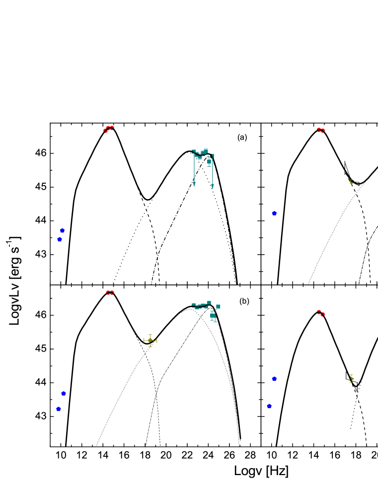
Figure 12: Modeling the four simultaneous SEDs. Blue pentagons are the radio observations from UMRAO. Red filled circles are the optical and NIR photometric data. The error bars for radio and optical fluxes are too small to be seen. Yellow diamond in (b) is the interpolation by nearby RXTE/PCA observations. The X-ray spectra with yellow triangles is from Swift/XRT. The cyan squares are the Fermi/LAT observations. The dash lines represent the calculated synchrotron emissions, the dot lines correspond to the SSC components and the dash dot lines are the ERC parts. (a) is the SED at 2008 Dec. with the strongest optical flare and a $\gamma$-ray flare with medium peak flux. (b) represents the SED at 2009 Oct. when both optical and $\gamma$-ray peak fluxes are in high state. (c) corresponds with a multi-wavelength flaring state at 2009 Dec. but the peak flux of $\gamma$-ray flare is extreme low. (d) is the SED that all bands are in low state at 2010 Jan.

The input parameters from modeling the simultaneous SEDs are shown in Table 3 and the fit results are shown in Figure 12. Four simultaneous SEDs are well described by the SSC+ERC model, which agrees with the result of similar simultaneous SED modeling work from Rani et al. (2013a). The variability phenomenon can be explained by the leptonic model. For S5 0716+714, its V band emission is likely around the synchrotron peak while the SSC emission peaks at about 10 MeV which is $\sim$1 order of magnitude lower than the energy range of Fermi/LAT, 0.1-300 GeV. When the frequencies of IC peaks become lower, the GeV $\gamma$-ray flux detected by LAT descends quickly. However, the V band emission can not be influenced seriously by a little change of synchrotron peak frequency because the SED slope is flat around synchrotron peak. Flares at 55107.7 and 55187.7 MJD are used to make a contrast. The input parameters at Table 3 are used. Since $\nu_{syn}\propto\gamma_{\rm br}^{2}B\delta$ and $\nu_{ssc}\simeq\gamma_{\rm br}^{2}\nu_{syn}$, the frequency of synchrotron peak in former flare is roughly 1.2 times as the latter, while for the frequencies of SSC peaks, it is about 2.8 times. It accords with the observations that the optical peak fluxes are almost same while the change of $\gamma$-ray peak fluxes is nearly three times.

The Doppler factors of three $\gamma$-ray flares trend to have higher values comparing to the low state. It corresponds with the VLBA observation that $\gamma$-ray flare always accompanys with apparent super-luminal knot ejection. The magnetic field intensities of these three $\gamma$-ray flares also trend to have higher values than the low state. The highest magnetic field intensity value is found in the flare at December 2009 when a extreme high PD of $(25.69\pm 0.80)$% is detected. For the three $\gamma$-ray flares, the $\gamma$-ray fluxes seem to be inversely proportional to magnetic field intensity values and proportional to the the Doppler factor values. However, the latter becomes marginal due to the fitting errors. These two tendencies are similar to the finding for 3C 454.3 (Bonnoli et al. 2011) and 3C 279 (Zhang et al. 2013).

6 DISCUSSIONS

Due to the absence of emission lines in the optical spectra of S5 0716+714, its redshift has not been exactly determined. In the above SED modeling, we took $z=0.31\pm 0.08$ ($1\sigma$ error) from Nilsson et al. (2008). Different radiation models are distinguished by the input model parameters which depend on the redshift. We attempt to discuss the possible influence caused by the uncertainty of the redshift. We take the SSC+ERC model with the hot dust emission as an example. 11 redshift points are chosen evenly in range of the uncertainty of reshift (0.23,0.39). We model the 11 SEDs with different redshifts independently. The B and $\delta$ distributions of the reshift are shown in Figure 13. The influence of $1\sigma$ uncertainty of reshift on B is comparable with the $1\sigma$ fit error. However, it is larger than the fit error on $\delta$. We also check the redshift influence on the pure SSC model and the SSC+ERC model using BLR emission. Including the influence of $1\sigma$ uncertainty of reshift, the tendency that input parameters from the pure SSC model are more extreme than the SSC+ERC models, is not changed.

To avoid the extreme input parameters from the pure SSC model, SSC+ERC models are used instead. On the other side, the assumption of the existence of the external emissions can not conflict with any observations of S5 0716+714. The luminosity of the presumed external emissions can not excess the nearby non-thermal jet emission. As few information of the accretion system is known, the characteristic radius scales of the dust torus $R_{dust}\sim 1$ pc and the BLR $R_{Ly\alpha}\sim 0.01$ pc are used, then

$$L_{dust,Ly\alpha}\simeq 4\pi R_{dust,Ly\alpha}^{2}cU_{dust,Ly\alpha},$$ (8)

where $U_{dust,Ly\alpha}$ is the energy density of the dust or Ly$\alpha$ line emission, and $c$ is the speed of light. The energy densities of the external field emissions are obtained from the average SED modeling, $U_{dust}\simeq 1.1\times 10^{-6}$ erg $\rm cm^{-3}$ and $U_{Ly\alpha}\simeq 8.6\times 10^{-6}$ erg $\rm cm^{-3}$, at observational frame. So the $L_{dust}$ and $L_{Ly\alpha}$ are calculated as $4.0\times 10^{42}$ and $3.1\times 10^{39}$ erg $\rm s^{-1}$, respectively. The non-thermal luminosity at the frequency of the maximum hot dust emission is about $1.7\times 10^{46}$ erg $\rm s^{-1}$ (Chen & Shan 2011). The constraint of the Ly$\alpha$ line luminosity has been recently obtained, L(Ly$\alpha)\lesssim 6.5\times 10^{41}$ erg $\rm s^{-1}$ (Danforth et al. 2013). So the luminosities of the external emissions are lower than the nearby non-thermal luminosities, which makes our assumption harmonious.

Strong $\gamma$-ray emissions from S5 0716+714 have been detected by MAGIC and Fermi. If the absorptions for $\gamma$-rays caused by the assumed external emissions are significant, the $\gamma$-ray photons can not escape, which conflicts with the $\gamma$-ray observations. The optical depth of photon-photon absorption between the $\gamma$-rays and the external emission can be simply calculated as (Dondi & Ghisellini 1995),

$$\tau_{\gamma\gamma}(x^{{}^{\prime}})=\frac{\sigma_{T}}{5}n^{{}^{\prime}}(x^{{}^{\prime}}_{t})x^{{}^{\prime}}_{t}R^{{}^{\prime}},$$ (9)

where $\sigma_{T}$ is the scattering Tomson cross-section, $n^{{}^{\prime}}(x^{{}^{\prime}}_{t})$ is the number density of target photon, $x^{{}^{\prime}}_{t}$ is the energy of target photon in dimensionless units and the $R^{{}^{\prime}}$ is the absorption length. The doubling time of 21 hours is used to constrain the emission region. The absorption length is considered the same as the distance between black hole and the emission blob (Celotti et al. 1998). $R^{{}^{\prime}}\simeq R_{\gamma}=ct_{var}\delta^{2}(1+z)^{-1}$. No matter the external seed photons are from the dust or Ly$\alpha$ line emission, the absorption opacity $\tau_{\gamma\gamma}\leq 10^{-6}\ll 1$. The absorptions are negligible. The assumptions of the external emission do not conflict with the $\gamma$-ray observations.

Synchrotron plus SSC+ERC models can well describe the broadband emission of S5 0716+714. Similar results are found in serval LBLs/IBLs. For BL Lacertae, the prototype of the BL Lac objects, shows that the SSC+ERC model using the BLR emission as seed photons is better than a two-zone SSC model and the pure SSC model is likely to be ruled out, acting like a FSRQ (Abdo et al. 2011). The SSC+ERC model with external IR seed photons can accord with the intraday variability for the 3C 66A (Reyes et al 2011), and get a more reasonable magnetic field parameter for W Comae (Acciari et al. 2009). Actually, any evidence of the thermal emission has not been found for S5 0716+714 and 3C 66A. However, the external seed photons are probably necessary to explain their $\gamma$-ray emissions. LBLs/IBLs, unlike the typical HBLs which can usually be simply well explained by single synchrotron plus SSC model (e.g. Bartoli et al. 2012), or the FSRQs whose the $\gamma$-ray emissions are often dominated by the ERC process (e.g. Bonnoli et al. 2011), are the kind of sources that both of the SSC and ERC processes may be indispensable for their $\gamma$-ray emissions.

7 CONCLUSIONS

We present the results of the radio to $\gamma$-ray observations of S5 0716+714, together with our photometric observations at Yunnan Observatories. The variations of the 14.5 GHz and hard X-ray emissions are correlated with zero-lag, which strongly supports the leptonic models. A coincidence of $\gamma$-ray and V band flares with a dramatic change of the optical PA at 2011 March is detected. $\gamma$-ray and V band flares at 2009 December correspond to a flare of optical PD. The V band and $\gamma$-ray flux variations are also correlated with zero-lag, consistent with the results of Rani et al. (2013a) and Larionov et al. (2013). A tight relationship between the optical and $\gamma$-ray emissions is suggested. The variability amplitudes in $\gamma$-ray and optical bands are higher than those in the hard X-ray and radio bands. The radiation cooling time of the high energy electrons which radiate the optical and $\gamma$-ray emissions is much shorter than it of the low energy electrons which produce the hard X-ray and radio emissions. The characteristic timescales of 14.5 GHz, optical, X-ray, and $\gamma$-ray bands from our ACF analysis are comparable to each other, which are consistent with results of the SF analysis of Rani et al. (2013a,b) that the characteristic timescales of radio, optical and $\gamma$-ray are $\sim$60-90 days. Variability of these bands are likely from the same origin which could be the change of properties of the radiating electrons. Hadronic models do not have the same nature explanation for these observations than the leptonic models. By comparing the optical light curve, “orphan” $\gamma$-ray flare which supports the hadronic models is not found. However, we find a peculiar phenomenon that a strong optical flare correlates a $\gamma$-ray flare whose peak flux is lower than the average flux. Leptonic model can explain this variability phenomenon through simultaneous SED modeling. Conclusively, the multi-wavelength emissions of S5 0716+714 are likely generated from the relativistic electrons.

Different leptonic models are distinguished by the average SED modeling. The pure SSC model is ruled out due to the extreme input parameters, according with result of Danforth et al. (2013) that the pure SSC model is different to explain the extreme fast optical variability. SSC+ERC model, whether the BLR or the hot dust emission is used as the external emission for the IC process, can well represent the SEDs and provide reasonable input parameters. It agrees with Rani et al. (2013a) which suggests that the SSC+EC model using BLR emission as the external photons provides a satisfactory description of the broadband SEDs. Including the influence of 1$\sigma$ uncertainty of the redshift of the source, the tendency that SSC+ERC models are more favorable than the pure SSC model has no change. The luminosities of the assumed external emissions do not excess the luminosities of nearby jet continuous emissions and the absorptions for $\gamma$-rays caused by the assumed external emissions are negligible, which makes our assumptions harmonious. Both SSC and ERC processes are probably needed to explain the $\gamma$-ray emission of S5 0716+714.

Figure 8: The ZDCFs (discrete points) and their fits (fifth-order polynomial least-squares fit, solid line).

Figure 13: The distributions of the B and $\delta$ with different values of redshift. 11 redshift points are chosen evenly in the 1$\sigma$ uncertainty of S5 0716+714 from Nilsson et al. (2008). The values of the B and $\delta$ are obtained by modeling 11 SEDs with different redshift independently using the SSC+ERC model with hot dust emission as the external photons.

Table 1: Results of Swift spectral fits during different state

					Flux
Model	$\Gamma_{1}$	$E_{\rm break}$(keV)	$\Gamma_{2}$	$\chi^{2}_{\nu}$/dof	(0.3–10 keV)
		2009-11-30 to 2009-12-02 (outburst)
Single power law	$2.30^{+0.14}_{-0.14}$	–	–	1.27/33	2.71
		2009-12-07 to 2009-12-22 (falling)
Single power law	$2.21^{+0.03}_{-0.03}$	–	–	1.36/102	1.60
Broken power law	$2.32^{+0.06}_{-0.06}$	$1.27^{+0.34}_{-0.23}$	$2.09^{+0.06}_{-0.07}$	1.26/100	1.66
Double power law	$2.32^{+0.71}_{-0.10}$	–	$0.92^{+2.11}_{-0.92}$	1.29/100	1.69
		2009-12-28 to 2010-02-22 (quiet)
Single power law	$2.33^{+0.24}_{-0.23}$	–	–	1.39/21	0.12
		2011-07-14 to 2011-07-16
Single power law	$2.09^{+0.15}_{-0.14}$	–	–	1.42/69	1.66
Broken power law	$2.49^{+0.51}_{-0.23}$	$3.26^{+0.52}_{-1.07}$	$1.17^{+0.56}_{-0.44}$	1.20/67	2.30
Double power law	$0.71^{+0.84}_{-1.79}$	–	$3.31^{+1.73}_{-0.84}$	1.18/67	3.76
		2011-10-25 to 2011-10-28
Single power law	$2.82^{+0.26}_{-0.23}$	–	–	1.96/46	1.33
Broken power law	$3.88^{+0.66}_{-0.55}$	$2.21^{+0.58}_{-0.35}$	$1.85^{+0.43}_{-0.58}$	1.51/44	4.04
Double power law	$1.40^{+0.71}_{-1.05}$	–	$5.06^{+1.84}_{-1.27}$	1.65/44	1.36

Table 2: The fractional variability amplitudes $F_{\rm{var}}$ for radio, infrared, optical, X-ray, and $\gamma$-ray light curves

4.8 GHz	8GHz	15 GHz	J-band	V-band	X-ray	Fermi
(1)	(2)	(3)	(4)	(5)	(6)	(7)
$0.25\pm 0.03$	$0.29\pm 0.03$	$0.31\pm 0.02$	$0.40\pm 0.02$	$0.38\pm 0.02$	$0.28\pm 0.05$	$0.52\pm 0.04$

Table 3: Input Parameters of the SED Model

Parameters	Pure SSC	SSC+ERC(BLR)	SSC+ERC(dust)	Dec.2008	Oct.2009	Dec. 2009	Jan. 2010
B(Gauss)	$6_{+1}^{-2}\times 10^{-3}$	$0.28_{+0.02}^{-0.02}$	$0.24_{+0.02}^{-0.01}$	$0.34_{+0.06}^{-0.05}$	$0.22_{+0.05}^{-0.03}$	$0.48_{+0.1}^{-0.07}$	$0.19_{+0.03}^{-0.03}$
$\delta$	$39.6_{+3.8}^{-3.1}$	$23.3_{+0.7}^{-0.9}$	$24.5_{+0.6}^{-0.7}$	$27.0_{+4.8}^{-3.1}$	$28.0_{+2.7}^{-3.0}$	$24.1_{+2.3}^{-1.7}$	$20.3_{+2.0}^{-1.4}$
$t_{var}$(day)	10	1	1	1	1	1	1
R(cm)	$7.8\times 10^{17}$	$4.6\times 10^{16}$	$4.8\times 10^{16}$	$5.3\times 10^{16}$	$5.5\times 10^{16}$	$4.8\times 10^{16}$	$4.0\times 10^{16}$
K	$1.2\times 10^{3}$	$1.1\times 10^{4}$	$1.0\times 10^{4}$	$0.1\times 10^{3}$	$1.4\times 10^{3}$	$1.3\times 10^{3}$	$0.9\times 10^{3}$
$\gamma_{br}$	$2.0\times 10^{4}$	$3.3\times 10^{3}$	$3.5\times 10^{3}$	$4.0\times 10^{3}$	$4.7\times 10^{3}$	$3.1\times 10^{3}$	$4.8\times 10^{3}$
$p_{1}$	2.4	2.2	2.2	1.7	2.0	2.0	1.8
$p_{2}$	3.9	3.8	3.8	4.6	4.2	4.2	4.5

Appendix A The multi-bands photometric data from Yunnan Observatories

Table 4: The multi-bands photometric data from Yunnan Observatories

MJD	Mag.	SigMag.	Band
54731.9	12.674	0.009	I
54733.9	12.563	0.016	I

References

- (1)
- (2) Abdo, A. A., Ackermann, M., Ajello, M., et al. 2009, ApJ, 700, 597
- (3)
- (4) Abdo, A. A., Ackermann, M., Agudo, I., et al. 2010a, ApJ, 716, 30
- (5)
- (6) Abdo, A. A., Ackermann, M., Ajello, M., et al. 2010b, ApJS, 188, 405
- (7)
- (8) Abdo, A. A., Ackermann, M., Ajello, M., et al. 2010c, ApJ, 710, 1271
- (9)
- (10) Abdo, A. A., Ackermann, M., Ajello, M., et al. 2010d, ApJ, 715, 429
- (11)
- (12) Abdo, A. A., Ackermann, M., Ajello, M., et al. 2010e, Nature, 463, 919
- (13)
- (14) Abdo, A. A., Ackermann, M., Ajello, M., et al. 2011, ApJ, 730, 101
- (15)
- (16) Acciari, V. A., Aliu, E., Aune, T., et al. 2009, ApJ, 707, 612
- (17)
- (18) Ackermann, M., Ajello, M., Allafort, A., et al. 2011, ApJ, 743, 171
- (19)
- (20) Aharonian, F, A., 2000, New Astron., 5, 377
- (21)
- (22) Albert, J., Aliu, E., Anderhub, H., et al. (The MAGIC Collaboration) 2008, ApJ, 674, 1037
- (23)
- (24) Aller, H. D., Aller, M. F., Latimer, G. E., & Hodge, P. E. 1985, ApJS, 59, 513
- (25)
- (26) Aller, M. F., Aller, H. D., Hughes, P. A., & Latimer, G. A. 1999, ApJ, 512, 601
- (27)
- (28) Alexander, T. 1997, in Astronomical Time Series, ed. D. Maoz, A. Sternberg, & E. M. Leibowitz (Dordrecht: Kluwer), 163
- (29)
- (30) Anderhub, H., Antonelli, L. A., Antoranz, P., et al. 2009, ApJ, 704, L129
- (31)
- (32) Atwood, W. B., Abdo, A. A., Ackermann, M., et al. 2009, ApJ, 697,1071
- (33)
- (34) Bach, U., Krichbaum, T. P., Ros, E., et al. 2005, A&A, 433, 815
- (35)
- (36) Bai, J. M., Xie, G. Z., Li, K. H., Zhang, X., & Liu, W. W. 1998, A&AS, 132, 83
- (37)
- (38) Bai, J. M., Xie, G. Z., Li, K. H., Zhang, X., & Liu, W. W. 1999, A&AS, 136,455
- (39)
- (40) Bartoli, B., Bernardini, P., Bi, X. J., et al., 2012, ApJ, 758, 2
- (41)
- (42) Beall, J. H., & Bednarek, W. 1999, ApJ, 510, 188
- (43)
- (44) Begelman, M. C., Fabian A. C.,& Rees, M. J., 2008, MNRAS, 384, L19
- (45)
- (46) Bessell, M. S., 2005, ARA&A, 43, 293
- (47)
- (48) Blandford RD, Rees MJ. 1978 In , ed.AM Wolfe, pp328-41. Pittsburgh: Univ. Pittsburgh Press
- (49)
- (50) Błażejowski, M., Sikora, M., Moderski, R., & Madejski, G. M. et al., 2000, ApJ, 545, 107
- (51)
- (52) Biermann, P., Duerbeck, H., Eckart, A., et al. 1981, ApJ, 247, L53
- (53)
- (54) Bonning, E., Urry, C. M., Bailyn, C., et al., 2012, ApJ, 756, 13
- (55)
- (56) Bonnoli, G., Ghisellini, G., Foschini, L., Tavecchio, F., & Ghirlanda, G. 2011, MNRAS, 410, 368
- (57)
- (58) Böttcher, M. 2005, ApJ, 621, 176
- (59)
- (60) Cappi, M., Comastri, A., Molendi, S., et al. 1994, MNRAS, 271,438
- (61)
- (62) Celotti, A., Fabian, A., & Rees, M., 1998, MNRAS, 293, 239
- (63)
- (64) Chandra, S., Baliyan, K. S., Ganesh, S., & Joshi, U. C. et al. 2011, ApJ, 731, 118
- (65)
- (66) Chatterjee, R., Bailyn, C. D., Bonning, E. W., et al. 2012, ApJ, 749, 191
- (67)
- (68) Chen, A. W., D’Ammando, F., Villata, M., et al. 2008, A&A, 489, L37
- (69)
- (70) Chen, P. S., & Shan, H. G., 2011, ApJ, 732, 22
- (71)
- (72) Danforth, C. W., Nalewajko, K., France, K., et al., 2013, ApJ, 764, 57
- (73)
- (74) Dermer, C, D., Schlickeiser, R., 1993, ApJ, 416, 458
- (75)
- (76) Dondi, L., Ghisellini, G., 1995, MNRAS, 273, 583
- (77)
- (78) Edelson, R. A., & Krolik, J. H. 1988, ApJ, 333, 646
- (79)
- (80) Edelson, R., Turner, T. J., Pounds, K., Vaughan, S., Markowitz, A., Marshall, H., Dobbie, P., Warwick, R., 2002, ApJ, 568, 610
- (81)
- (82) Fuhrmann, L., Krichbaum, T. P., Witzel, A., et al. 2008, A&A, 490, 1019
- (83)
- (84) Ghisellini, G., Villata, M., Raiteri, C. M., et al. 1997, A&A, 327, 61
- (85)
- (86) Ghisellini, G., Tavecchio, F., Foschini, L., et al. 2010, ApJ, 402, 497
- (87)
- (88) Giommi, P., Massaro, E., Chiappetti, L., et al. 1999, A&A, 351, 59
- (89)
- (90) Giommi, P., Colafrancesco, S., Cutini, S., et al. 2008, A&A, 487, L49
- (91)
- (92) Giveon, U., Maoz, D., Kaspi, S., Netzer, H., & Smith, P. S. 1999, MNRAS, 306, 637
- (93)
- (94) Hartman, R. C., Bertsch, D. L., Bloom, S. D., et al. 1999, ApJS, 123, 79
- (95)
- (96) Ikejiri, Y., et al. 2009, in Proc. 2009 Fermi Symp., arXiv:0912.3664
- (97)
- (98) Ikejiri, Y., Uemura, M., Sasada, M., et al. 2011, PASJ, 63, 639
- (99)
- (100) Kraus, A., Krichbaum, T. P., Wegner, R., et al. 2003, A&A, 401,161
- (101)
- (102) Komatsu, E., Smith, K. M., Dunkley, J., et al. 2011, ApJS, 192, 18
- (103)
- (104) Kühr, H., Witzel, A., Pauliny-Toth, I. I. K., & Nauber, U. 1981, A&AS, 45, 367
- (105)
- (106) Larionov, V., Konstantinova, T., Kopatskaya, E., et al. 2008, ATel, 1502
- (107)
- (108) Larionov, V. M., Jorstad, S. G., Marscher, A. P., et al. 2013, ApJ, 768, 40
- (109)
- (110) Lin, Y. C., Bertsch, D. L., Dingus B. L., et al. 1995, ApJ, 442, 96
- (111)
- (112) Liu, H. T., Bai, J. M., Zhao X. H., & Ma, L. 2008, ApJ, 677, 884
- (113)
- (114) Liu, H. T., Bai, J. M., Wang, J. M., 2011, MNRAS, 414, L155
- (115)
- (116) Liu, H. T., Bai, J. M., Wang, J. M., Li, S. K. 2011, MNRAS, 418, L90
- (117)
- (118) Malmrose, M. P., Marscher, A. P., Jorstad, S. G., Nikutta, R., & Elitzur, M. et al., 2011, ApJ, 732, 116
- (119)
- (120) Maraschi,L., Celotti, A., Ghisellini, G., 1992, ApJ, 298, 114
- (121)
- (122) Marscher, A. P., Jorstad, S. G., D’Arcangelo, F. D., et al. 2008, Nature, 452, 966
- (123)
- (124) Mattox, J. R., Bertsch, D. L., Chiang, J., et al., 1996, ApJ, 461, 396
- (125)
- (126) Mücke, A., & Protheroe, R, J., 2001, Astropart, Phys., 15, 121
- (127)
- (128) Murphy, E.M., Lockman, F.J., Laor, A., & Elvis, M. 1996, ApJS, 105, 369
- (129)
- (130) Netzer, H., Heller, A., Loinger, F., et al. 1996, MNRAS, 279, 429
- (131)
- (132) Nolan, P. L., Abdo, A. A., Ackermann, M., et al 2012, ApJS, 199, 31
- (133)
- (134) Nesci, R., Massaro, E., Rossi, C., et al. 2005, AJ, 130, 1466
- (135)
- (136) Nilsson, K., Pursimo, T., Sillanpää, A., Takalo, L. O., & Lindfors, E. et al. 2008, A&A, 487, L29
- (137)
- (138) Padovani, P., & Giommi, P. 1995, ApJ, 444, 567
- (139)
- (140) Poon, H., Fan, J. H., & Fu, J. N., 2009, ApJS, 185, 511
- (141)
- (142) Raiteri, C. M., Villata, M., Tosti, G., et al. 2003, A&A, 402, 151
- (143)
- (144) Rani, B., Krichbaum, T. P., Fuhrmann, L., et al. 2013a, A&A, 552, 11
- (145)
- (146) Rani, B., Krichbaum, T. P., Lott, B., Fuhrmann, L., & Zensus, J. A., 2013B, Advances in Space Research, 51, 2358
- (147)
- (148) Reyes L. C., Abdo, A. A., Ackermann, M., Ajello, M., et al. 2011, ApJ, 726, 43
- (149)
- (150) Schlegel, D. J., Finkbeiner, D. P., & Davis, M. 1998, ApJ, 500,525
- (151)
- (152) Shaw, M. S., Romani, R. W., Healey, S. E., et al., 2009, ApJ, 704, 477
- (153)
- (154) Sikora, M., Begelman, M., & Rees, M., 1994, ApJ, 421,153
- (155)
- (156) Sikora, M., Stawarz, Ł., Moderski, R., Nalewajko, K., & Madejski, G. M. 2009, ApJ, 704, 38
- (157)
- (158) Sambruna, R. M., 2007, ApS&S, 311, 241
- (159)
- (160) Smith, P.S., Montiel, E., Rightley, S., Turner, J., Schmidt, G.D., & Jannuzi, B.T. 2009, arXiv:0912.3621, 2009 Fermi Symposium, eConf Proceedings C091122.
- (161)
- (162) Soldi, S., Türler, M., Paltani, S., et al. 2008, A&A, 486, 411
- (163)
- (164) Tagliaferri, G., Ravasio, M., Ghisellini, G., et al., 2003, A&A, 400, 477
- (165)
- (166) Takalo, L. O., Sillanpaeae, A., & Nilsson, K. 1994, A&AS, 107, 497
- (167)
- (168) Tavani, M., Barbiellini, G., et al. 2008, NIMPA, 588, 52
- (169)
- (170) Tavecchio, F., Maraschi, L., & Ghisellini, G., 1998, ApJ, 509, 608
- (171)
- (172) Trevese, D., Kron, R. G., Majewski, S. R., Bershady, M. A., & Koo, D. C. 1994, ApJ, 433, 494
- (173)
- (174) Ulrich, M.-H., Maraschi, L., & Urry, C. M. 1997, ARA&A, 35, 445
- (175)
- (176) Urry, C. M.,& Padovani, P. 1995, PASP, 107, 803
- (177)
- (178) Vaughan, S., Edelson, R., Warwick, R. S., Uttley, P. 2003, MNRAS, 345, 1271
- (179)
- (180) Villata, M., Raiteri, C. M., Lanteri, L., Sobrito, G., & Cavallone, M. 1998, A&AS, 130, 305
- (181)
- (182) Villata, M., Raiteri, C. M., Larionov, V. M., et al. 2008, A&A, 481, L79
- (183)
- (184) von Montigny, C., Bertsch, D. L., Chiang, J., et al. 1995, ApJ, 440, 525
- (185)
- (186) Wagner, S. J., & Witzel, A., 1995, ARA&A, 33, 163
- (187)
- (188) Wagner, S. J., Witzel, A., Heidt, J., et al. 1996, AJ, 111, 2187
- (189)
- (190) Weng, S. S., & Zhang, S. N. 2011, ApJ, 739, 42
- (191)
- (192) Zhang, Y. H. 2010, ApJ, 713, 180
- (193)
- (194) Zhang, J., Liang, E.-W., Zhang, S.-N., & Bai, J. M. et al., 2012, ApJ, 752, 157
- (195)
- (196) Zhang, J., Zhang, S.-N., & Liang, E.-W. 2013, ApJ, 767, 8