The impact of the ghost-gluon vertex on the ghost Schwinger-Dyson equations

Abstract:

We derive an approximate dynamical equation for the form-factor of the ghost-gluon vertex that contributes to the Schwinger-Dyson equation of the ghost dressing function in the Landau gauge. In particular, we consider the “one-loop dressed” approximation of the corresponding equation governing the evolution of the ghost-gluon vertex, using fully dressed propagators and tree-level vertices in the relevant diagrams. Within this approximation, we then compute the aforementioned form factor for two special kinematic configurations, namely the soft gluon limit, in which the momentum carried by the gluon leg is zero , and the soft ghost limit, where the momentum of the anti-ghost leg vanishes. The results obtained display a considerable departure from the tree-level value, and are in rather good agreement with available lattice data. We next solve numerically the coupled system formed by the equation of the ghost dressing function and that of the the vertex form factor, in the soft ghost limit. Our results demonstrate clearly that the nonperturbative contribution from the ghost-gluon vertex accounts for the missing strength in the kernel of the ghost equation, and allows for an impressive coincidence with the lattice results, without the need to artificially enhance the coupling constant of the theory.

1 Introduction

A qualitative and quantitative understanding of fundamental Green’s function in the infrared (IR) sector constitutes a long-standing challenge in QCD. In the last few years, our knowledge of the QCD low energy regime has advanced considerably, due to a systematic efforts obtained through various non-perturbative methods, such as by lattice simulations [1, 2, 3, 4, 5, 6], Schwinger-Dyson equations (SDEs) [7, 8, 9, 10, 11], functional methods [12, 13, 14], and algebraic techniques [15, 16, 17]. On the level of the two-point Green’s functions, it is by now well-established that, in the Landau gauge, the gluon propagator and the ghost dressing function are finite in the IR [7, 9]. The finiteness of both quantities are associated to the phenomenon of dynamical gluon mass generation [18, 19, 20, 21, 22, 7].

Although, we have a qualitative understanding of the origin of the finiteness of the ghost dressing function, $F(p^{2})$, it has been more difficult to obtain from a self-consistent SDE analysis its entire shape and size provided by the lattice [7, 23, 24].

More specifically, when we substitute the gluon propagator furnished by the lattice into the ghost SDE, but keeping the ghost-gluon vertex at its tree-level value, the resulting $F(p^{2})$ is significantly suppressed compared to that of the lattice [7]; to reproduce the lattice result, one has to artificially increase the value of the gauge coupling from the correct value $\alpha_{s}=0.22$ to $\alpha_{s}=0.29$ [25] as illustrated in the Fig. 1.

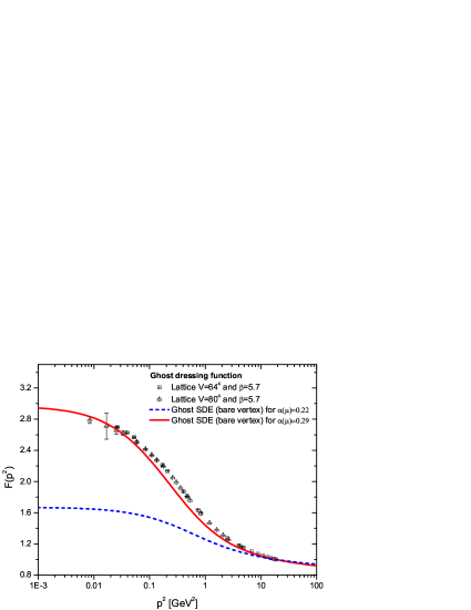
Figure 1: Comparison of the ghost dressing function, $F(p^{2})$, obtained as solution of the ghost SDE when the ghost-gluon vertex is approximate by its bare value, with the lattice data of Ref. [3]. The (red) continuous curve represents the case when $\alpha_{s}(4.3\,\rm GeV)=0.29$ whereas the (blue) dashed curve is obtained when $\alpha_{s}(4.3\,\rm GeV)=0.22$.

Given the simple structure of the ghost SDE, it is become clear that the origin of the observed discrepancy is due to the tree-level approximation we impose for the fully dressed ghost-gluon vertex, $\Gamma_{\nu}$ [26].

Even though preliminary lattice studies indicate that the deviations of $\Gamma_{\nu}$ from its tree-level value are relatively moderate [27, 28, 29, 30], it is natural to expect that, due to the nonlinear nature of SDE, that even a small deviation can generate significant effects on the kernel of the equation that describes the behavior of the ghost dressing function. Similar studies on the influence of the three-point functions on the propagators can be found in Refs. [23, 31, 32, 33].

The main purpose of this talk is present the “one-loop dressed” version of the SDE satisfied by one of the form factors appearing in the definition of ghost-gluon vertex, $\Gamma_{\nu}$, in the Landau gauge.

To be more specific, the tensorial decomposition of $\Gamma_{\nu}$ consists of two form factors; however, due to the transversality of the gluon propagator present in the ghost SDE, written in Landau gauge, only the form factor $A(-k,-p,r)$ of the ghost momentum $p_{\nu}$ survives.

Here we present our results for $A(-k,-p,r)$ in two particular kinematic configurations: (i) soft gluon ($k\to 0$) and (ii) soft ghost ($p\to 0$). For the first case, we compare our results with the lattice data of Ref. [28, 29]. The second configuration is the relevant one for the ghost SDE. Therefore, we solve numerically the coupled system of integral equations formed by $F(p^{2})$ and $A(-k,0,k)$. The numerical solution obtained gives rise to a ghost dressing function that is in excellent agreement with the lattice data [3] using the standard value of the gauge coupling constant $\alpha_{s}=0.22$ which corresponds to the momentum-subtraction (MOM) value for the point $\mu=4.3$ GeV [34], used to renormalize the gluon propagator obtained from the lattice [26].

2 The ghost SDE and the ghost-gluon vertex

We start by denoting the full ghost-gluon vertex, shown in Fig. 2, by

$$\Gamma_{\nu}^{nbc}(-k,-p,r)=gf^{nbc}\Gamma_{\nu}(-k,-p,r)\,,\quad r=k+p\,,$$ (1)

with $k$ representing the momentum of the gluon and $p$ of the anti-ghost.

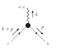
Figure 2: The fully dressed ghost-gluon vertex.

The most general Lorentz structure of this vertex is given by

$${\Gamma}_{\nu}(-k,-p,r)=A(-k,-p,r)\,p_{\nu}+B(-k,-p,r)\,k_{\nu}\,.$$ (2)

At tree-level, the two form factors assume the values $A^{[0]}(-k,-p,r)=1$ and $B^{[0]}(-k,-p,r)=0$, giving rise to the well know bare ghost-gluon vertex $\Gamma^{[0]}_{\nu}=p_{\nu}$.

It is convenient to define now the so-called “Taylor limit” of the ghost-gluon vertex, where the vertex has vanishing ghost momentum, $r=0$, $p=-k$. In this special kinematic configuration, the $\Gamma_{\nu}(-k,-p,r)$ of Eq. (2) becomes

$$\Gamma_{\nu}(-k,k,0)=-[A(-k,k,0)-B(-k,k,0)]k_{\nu}\,.$$ (3)

Intimately connected to this limit is the well-known Taylor theorem, which states that, to all orders in perturbation theory  [35]. ,

$$A(-k,k,0)-B(-k,k,0)=1;$$ (4)

as a result, the fully-dressed vertex assumes the tree-level value corresponding to this particular kinematic configuration, i.e., $\Gamma_{\nu}(-k,k,0)=-k_{\nu}$.

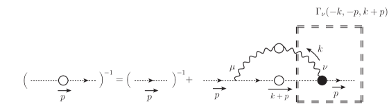
Figure 3: The SDE for the ghost propagator given by Eq. (2.5). The white blobs represent the fully dressed gluon and ghost propagators, while the black blob denotes the dressed ghost-gluon vertex.

Of extreme importance for this analysis is to understand how different behaviors for the ghost-gluon vertex affects the structure of the ghost SDE, diagrammatically represented in the Fig. 3, and written as

$$iD^{-1}(p^{2})=ip^{2}-g^{2}C_{\rm{A}}\int_{k}\Gamma_{\mu}^{[0]}(k,-k-p,p)\Delta^{\mu\nu}(k)\Gamma_{\nu}(-k,-p,k+p)D(k+p)\,,$$ (5)

where $C_{\rm A}$ denotes the Casimir eigenvalue of the adjoint representation ($N$ for $SU(N)$), $d=4-\epsilon$ is the space-time dimension, and we have introduced the integral measure

$$\int_{k}\equiv\frac{\mu^{\epsilon}}{(2\pi)^{d}}\!\int\!\mathrm{d}^{d}k,$$ (6)

with $\mu$ the ’t Hooft mass. In the Landau gauge, the gluon propagator $\Delta_{\mu\nu}(q)$ has the transverse form

$$\Delta_{\mu\nu}(q)=-iP_{\mu\nu}(q)\Delta(q^{2})\,\quad\mbox{with}\quad P_{\mu\nu}(q)=g_{\mu\nu}-\frac{q_{\mu}q_{\nu}}{q^{2}}\,.$$ (7)

Due to the full transversality of $\Delta_{\mu\nu}(k)$, any reference to the form factor $B$ disappears from the ghost SDE of Eq. (5). Specifically, substituting Eq. (2) into Eq. (5), and introducing the usual renormalization constants we obtain [26]

$$F^{-1}(p^{2})=Z_{c}+ig^{2}C_{\rm{A}}\int_{k}\,\left[1-\frac{(k\cdot p)^{2}}{k^{2}p^{2}}\right]A(-k,-p,k+p)\Delta(k)D(k+p)\,,$$ (8)

where we have introduced the ghost dressing function, $F(q^{2})$, defined as $F(q^{2})=q^{2}D(q^{2})$.

Notice that the closed expression of $Z_{c}$ is obtained from Eq. (8) itself, by imposing the MOM renormalization condition on $F(q^{2})$, i.e $F(q^{2}=\mu^{2})=1$, where $\mu$ is the renormalization point where the dressing function assumes its tree-level value.

Evidently, Eq. (8) couples the unknown functions $A(-k,-p,k+p)$, described by the corresponding vertex SDE, and $F(p^{2})$. Given that $A(-k,-p,k+p)$ is a function of three variables, $p^{2}$, $k^{2}$, and the angle between the two (appearing in the inner product $p\cdot k$), a full SDE treatment is rather cumbersome, and lies beyond our present technical powers. Instead, we will consider the behavior of $A(-k,-p,k+p)$ for vanishing $p$; to that end, we start out with the Taylor expansion of $A(-k,-p,k+p)$ around $p=0$, and we only keep the first term, $A(-k,0,k)$, thus converting $A$ into a function of a single variable. We emphasize that the limit $p\to 0$ is taken only inside the argument of the form factor $A$, but not in the rest of the terms appearing in the SDE of Eq. (8) [26].

Thus, the approximate version of the SDE in Eq. (8) reads

$$F^{-1}(p^{2})=Z_{c}+ig^{2}C_{\rm{A}}\int_{k}\,\left[1-\frac{(k\cdot p)^{2}}{k^{2}p^{2}}\right]A(-k,0,k)\Delta(k)D(k+p)\,.$$ (9)

3 The one-loop dressed approximation for the vertex

In this section, we will schematize the derivation of the nonperturbative expression for the form factor $A$, in two special kinematic configurations: (i) the soft gluon limit, in which the momentum carried by the gluon leg is zero ($k=0$), and (ii) the soft ghost limit, where the momentum of the anti-ghost leg vanishes ($p=0$).

To do that, we start by showing in Fig. 4 the diagrammatic representation of the SDE satisfied by the ghost-gluon vertex. Besides the full gluon and ghost propagators, we observe that the most relevant quantity, which controls the dynamics of this vertex, is the four-point ghost-gluon kernel represented by the gray blob.

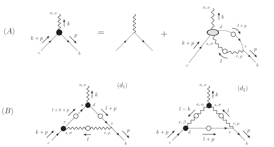
Figure 4: (A) The complete SDE of the ghost-gluon vertex. (B) The diagrams that contributes to the ghost-gluon vertex SDE after the “one-loop dressed” expansion of the ghost-gluon kernel.

In order to derive a SDE for the ghost-gluon vertex tractable, we will replace the ghost-gluon kernel by its “one-loop dressed” approximation [36]. In other words, the skeleton expansion of the four-point ghost-gluon kernel will only include the diagrams appearing in panel $(B)$ of Fig. 4.

Thus, the approximate version of the SDE that we employ may be cast in the form

$$\Gamma_{\nu}(-k,-p,k+p)=p_{\nu}-\frac{i}{2}g^{2}C_{\rm A}[(d_{1})_{\nu}-(d_{2})_{\nu}]\,,$$ (10)

where the diagrams $(d_{i})$ are given by

$$(d_{1})_{\nu} = \int_{l}\Gamma_{\rho}^{[0]}\Delta^{\rho\sigma}(l)\Gamma_{\sigma}D(l+k+p)\Gamma_{\nu}D(l+p)\,,$$

$$(d_{2})_{\nu} = \int_{l}\Gamma_{\rho}^{[0]}\Delta^{\rho\sigma}(l)\Gamma_{\nu\sigma\alpha}\Delta^{\alpha\beta}(l-k)\Gamma_{\beta}D(l+p)\,.$$ (11)

Moreover, in the two diagrams, $(d_{1})$ and $(d_{2})$, we will keep fully dressed propagators, but we will replace the fully dressed three-gluon vertex appearing in graph $(d_{2})$ by its tree-level expression, namely

$$\Gamma_{\alpha\mu\nu}(q,r,p)\rightarrow\Gamma_{\alpha\mu\nu}^{[0]}(q,r,p)=(r-p)_{\alpha}g_{\mu\nu}+(p-q)_{\mu}g_{\nu\alpha}+(q-r)_{\nu}g_{\alpha\mu}\,.$$ (12)

It is important to notice the presence of the fully dressed ghost-gluon vertices, in the diagrams, $(d_{1})$ and $(d_{2})$. In the sequence, we will mention the additional approximations will be imposed on those vertices, depending on the specific details of each kinematic case considered.

3.1 Soft gluon configuration

The first kinematic configuration we will analyse is the so-called soft gluon limit, where the gluon leg has a vanishing momentum, $k=0$. In this case the ghost-gluon vertex becomes a function of only one momentum, $p$, and it is entirely expressed in terms of a single form factor, namely,

$$\Gamma_{\nu}(0,-p,p)=A(p)p_{\nu};\quad A(p)\equiv A(0,-p,p)\,.$$ (13)

Setting $k=0$ in Eq. (10), one is able to isolate the form factor $A$ by means of the projection

$$A(p)=1-\frac{i}{2}g^{2}C_{A}[(d_{1})-(d_{2})];\quad(d_{i})\equiv\frac{p^{\nu}}{p^{2}}(d_{i})_{\nu}\,,\quad i=1,2\,,$$ (14)

where the diagrams $(d_{i})$ are obtained from those of Eq. (3) in the limit $k\rightarrow 0$.

Notice that in the limit $k=0$, the vertex $\Gamma_{\nu}$ entering in graph $(d_{1})$ becomes $\Gamma_{\nu}(0,-l-p,l+p)$, which allows one to derive a linear integral equation for the unknown quantity for $A(0,-p,p)$.

On the other hand, the same momenta configuration does not happen to the remaining ghost-gluon vertices, namely, $\Gamma_{\sigma}$ and $\Gamma_{\beta}$ in graphs $(d_{1})$ and $(d_{2})$, respectively; their arguments depend on all possible kinematic variables, and the inclusion of the full $A$ would give rise to a (non-linear) integral equation, too complicated to solve. We therefore approximate all remaining ghost-gluon vertices by their tree-level expressions.

Thus, using the notation introduced in Eq. (14), the diagram $(d_{1})$ reads

$$(d_{1})=\int_{l}\frac{(l\cdot p)}{(l+p)^{2}p^{2}}[(l\cdot p)^{2}-l^{2}p^{2}]D^{2}(l)\Delta(l+p)A(l)\,;$$ (15)

while $(d_{2})$ is given by

$$(d_{2})=2\int_{l}\frac{(l\cdot p)}{l^{2}p^{2}}[l^{2}p^{2}-(l\cdot p)^{2}]\Delta^{2}(l)D(l+p)\,.$$ (16)

Combining the above expressions, the final answer for $A(p)$, in Euclidean space, is given by [26]

$$A(x) = 1-\frac{\alpha_{s}C_{A}}{4\pi^{2}}\int_{0}^{\infty}\!\!\!dt\sqrt{xt}\,F^{2}(t)A(t)\int_{0}^{\pi}\!\!\!d\theta\sin^{4}\theta\cos\theta\left[\frac{\Delta(z)}{z}\right]$$ (17)

$$- \frac{\alpha_{s}C_{A}}{2\pi^{2}}\int_{0}^{\infty}\!\!\!dt\sqrt{xt}\,t\,\Delta^{2}(t)\int_{0}^{\pi}\!\!\!d\theta\sin^{4}\theta\cos\theta\left[\frac{F(z)}{z}\right]\,,$$

with $l^{2}=t$; $p^{2}=x$; $(l+p)^{2}=z$; $(l\cdot p)=\sqrt{xt}\cos\theta$. In addition, we have used $g^{2}=4\pi\alpha_{s}$, and re-express the ghost propagators in terms of their dressing functions.

It is interesting to notice that, when the momentum of the ghost leg is also zero, i.e. $x=0$, Eq. (17) reproduces the tree-level value of the form factor, i.e., $A(0)=1$.

3.2 Soft ghost configuration (Taylor kinematics)

Now, let us derive an approximate version for $A$ in the soft ghost configuration, to be denoted by

$$\lim_{p\rightarrow 0}A(-k,-p,k+p)=A(-k,0,k)\equiv A(k)\,.$$ (18)

As mentioned before, we will employ the soft ghost configuration into the ghost SDE and check the improvements, this configuration may make in the description of the IR behavior of the ghost dressing function.

It is important to emphasize here that the form factor $A(-k,0,k)$ obtained in the soft ghost configuration coincides with that of the Taylor kinematics $A(-k,k,0)$, appearing in the constraint imposed by Taylor’s theorem, given by Eq. (4). A detailed proof of the equivalence of $A(-k,0,k)=A(-k,k,0)$ can be found in Ref. [26].

Let us now derive the explicit expression for the form factor $A$ in the soft ghost limit. Again, your starting point are the diagrams shown in panel $(B)$ of Fig. 4, where we dress up all gluon and ghost propagators, and keep tree-level values for all the interaction vertices.

In this configuration, the expressions given in Eq. (3) reduce to

$$(d_{1})_{\nu} = p^{\rho}(k+p)^{\sigma}\int_{l}(l+p)_{\nu}D(l+p)D(l+k+p)\Delta(l)P_{\rho\sigma}(l)\,,$$

$$(d_{2})_{\nu} = p^{\rho}(k+p)^{\beta}\int_{l}D(l+p)\Delta(l)\Delta(l-k)P_{\rho}^{\sigma}(l)P^{\alpha}_{\beta}(l-k)\Gamma^{[0]}_{\nu\sigma\alpha}\,,$$ (19)

The general procedure for isolating the $A(-k,0,k)$ from the diagrams $(d_{1})$ and $(d_{2})$, must be done with care. Here, due to space limitations, we will only outline the basic steps that should be performed: (i) Set $p=0$ from the beginning inside the integrals of Eq. (3.2); (ii) Discard all the terms that give rise to structures of the type ${\cal O}(p)(k+p)_{\nu}$; (iii) Determine the contribution of the diagram that saturates the index of the momentum $p^{\rho}$ with the metric tensor $g_{\nu\rho}$. For more details see Ref. [26].

After performing the steps described above, we arrive at the final result (in Euclidean space)

$$A(y) = 1-\frac{\alpha_{s}C_{\rm A}}{12\pi^{2}}\int_{0}^{\infty}\!\!\!dt\,\sqrt{yt}\,F(t)\Delta(t)\int_{0}^{\pi}\!\!\!d\theta^{\prime}\sin^{4}\theta^{\prime}\cos\theta^{\prime}\left[\frac{F(u)}{u}\right]$$

$$+ \frac{\alpha_{s}C_{\rm A}}{6\pi^{2}}\int_{0}^{\infty}\!\!\!dt\,F(t)\Delta(t)\int_{0}^{\pi}\!\!\!d\theta^{\prime}\sin^{4}\theta^{\prime}\left[\frac{\Delta(u)}{u}\right][yt(1+\sin^{2}\theta^{\prime})-(y+t)\sqrt{yt}\cos\theta^{\prime}]\,.$$

where, in this case, $y=k^{2}$, $u=(l+k)^{2}$, and $\theta^{\prime}$ is the angle between $k$ and $l$.

4 Numerical result for the soft gluon configuration

Now we are in position to solve numerically the equations obtained in the previous sections. More specifically, in this section we determine $A(0,-p,p)$ by solving the integral equation (17) through an iterative process. To do that, we use as input the lattice data obtained from the $SU(3)$ quenched simulations of [3], renormalized at $\mu=4.3$ GeV, within the MOM scheme (see Fig. 5).

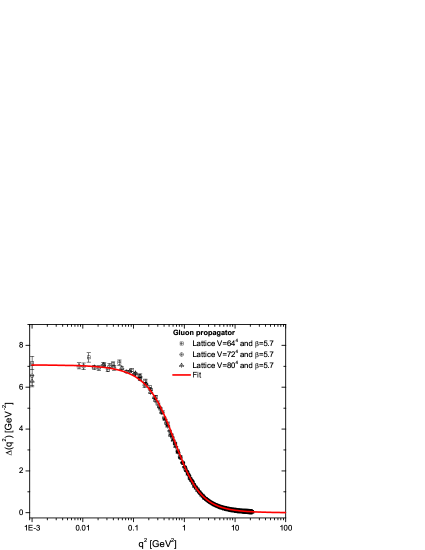
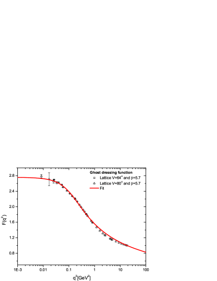
Figure 5: Lattice results for the gluon propagator, $\Delta(q)$, (left panel) and ghost dressing, $F(q)$, (right panel) obtained in Ref. [3] and renormalized at $\mu=4.3$ GeV.

In addition, we will employ $\alpha_{s}(\mu)=0.22$ that is the standard value for the gauge coupling obtained from the higher-order calculation presented in [34].

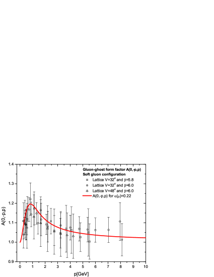
Figure 6: Comparison of our numerical result for $A(0,-p,p)$, obtained from Eq.(3.8) when $\alpha_{s}(\mu)=0.22$ (red line) and the lattice data of Ref. [28, 29].

Our result for the soft gluon configuration are presented in the Fig. 6, where the (red) curve represents the corresponding solution for $A(0,-p,p)$. Notice that $A(0,-p,p)$ develops a considerable peak around the momentum region of $830$ MeV. It is also interesting to notice that in both, IR and ultraviolet limits, the form factor $A$ gradually approaches its tree level value.

In the same Fig. 6, we compare our numerical results with the corresponding lattice data obtained in Ref. [28, 29] for this particular kinematic configuration.

Although, the error bars are rather pronounced, we clearly see that our solution follows the general structure of the data. In particular, notice that both peaks occur in the same intermediate region of momenta, where $A(0,-p,p)$ receives a significant non-perturbative correction, deviating considerably from its tree level value.

5 Numerical results for the coupled system

In this section, we solve numerically the coupled system formed by the integral equations of the ghost dressing function (9) and the one for the ghost-gluon vertex in the soft ghost configuration, given by (3.2). Here again, the unique external ingredient used when solving this system are the lattice data for the gluon propagator $\Delta(q)$ shown on the left panel of Fig.  5. In particular, we are interested in analysing how the inclusion of a non-trivial corrections for the corresponding ghost-gluon vertex induces modifications in the ghost dressing function.

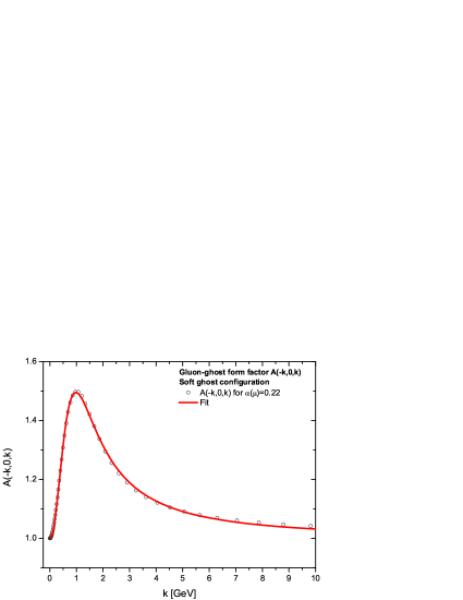
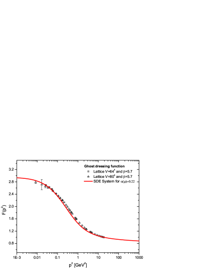
Figure 7: Left panel: The form factor $A(-k,0,k)$ (circles) and the fit given by Eq.(4.1) (red continuous line). Right panel: The numerical solution of $F(p)$ (red continuous line) compared with the lattice data of Ref. [3]. Note that the value of $\alpha_{s}$ used when solving the system is $\alpha_{s}(\mu)=0.22$.

The results for $F(p)$ and $A(-k,0,k)$ when $\alpha_{s}(\mu)=0.22$ are shown in Fig. 7. On the left panel, the circles represents our result for $A(-k,0,k)$. Here again, $A(-k,0,k)$ displays the same pattern found in the soft gluon configuration. More specifically, the peak reaches its maximum around $1$ GeV and the curve tends to its tree-level value in the IR and ultraviolet limits. Unfortunately, in this plot we do not compare our results with the lattice predictions, since there are no available lattice data for the ghost soft configuration.

The (red) continuous curve of Fig. 7, represents the fit for $A(-k,0,k)$, whose functional form is given by

$$A(-k,0,k)=1+\frac{ak^{2}}{[(k^{2}+b)^{2}+c]}\ln\big{(}d+k^{2}/k_{0}^{2}\big{)}\,,$$ (21)

where the adjustable parameters are $a=0.68\,\mbox{GeV}^{2}$, $b=0.72\,\mbox{GeV}^{2}$, $c=0.29\,\mbox{GeV}^{4}$, $d=9.62$ and $k_{0}^{2}=1\,\mbox{GeV}^{2}$.

The comparison of $F(p)$ (red continuous curve) obtained as solution from the system of Eqs. (9) and (3.2) with the lattice data of Ref. [3] are shown on the right panel of Fig. 7. As we can clearly see, we find a remarkable agreement between the curves, even keeping the standard value of the coupling constant, i.e. $\alpha_{s}(\mu)=0.22$.

From the results presented in Fig. 7, we can conclude that although $A(-k,0,k)$ is not very different from its value at tree level in the deep IR region, however, the presence of the peak, in its intermediate region, when integrated in the kernel of ghost SDE is sufficient for increasing the saturation point from $F(0)=1.67$ to $F(0)=2.95$ (see Figs. 1 and 7, respectively).

This observation suggests that the ghost SDE is particularly sensitive to the values of its ingredients at momenta around two to three times the QCD mass scale.

For the sake of completeness, we will repeat the same analysis for the $SU(2)$ gauge group. To do that, we set $C_{\rm A}=2$ in the system of Eqs. (9) and (3.2), and we solve the system using as input the $SU(2)$ data for $\Delta(q)$ of Ref. [1] renormalized at $\mu=2.2$ GeV, moreover we use the value $\alpha_{s}(\mu)=0.81$.

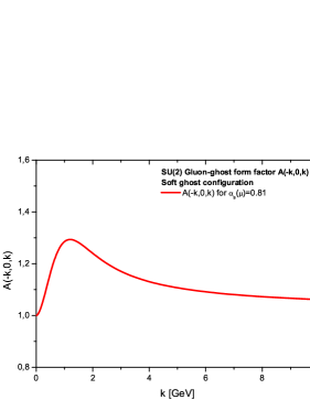
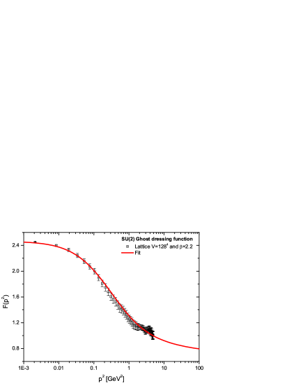
Figure 8: Left panel: The numerical result for $A(-k,0,k)$ obtained from the system of Eqs. (2.9) and (3.11) when $\alpha_{s}(\mu)=0.81$ (red continuous line). Right panel: Comparison of $F(p)$ (red continuous line) obtained from as solution from the coupled system with the $SU(2)$ lattice data of Ref. [1].

On the left panel of Fig. 8, we show our numerical results for $A(-k,0,k)$. Once again, we see that the solution displays the same qualitative behavior found in the $SU(3)$ analysis, shown in Fig. 7. However, for the $SU(2)$, the peak is slightly shifted towards to the ultraviolet, occurring at around $1.2$ GeV.

The result for $F(p)$ (red continuous curve) is presented on the right panel of Fig. 8. We clearly see, once more, the excellent agreement with the corresponding lattice data of [1].

Notice that also in the $SU(2)$ case, the introduction of the non-perturbative correction to the ghost-gluon vertex reduces considerably the value of the gauge coupling needed to reproduce the lattice data. Specifically, when we employ the bare vertex the lattice result is reproduced for $\alpha_{s}(\mu)=0.99$, whereas the value of the coupling used when solving the system of $F(p)$ and $A(-k,0,k)$ is $\alpha_{s}(\mu)=0.81$.

6 Conclusions

In this talk we have presented a study of the impact of the ghost-gluon vertex on the overall shape of dressing of the ghost propagator obtained as solution of the ghost SDE for different $SU(N)$ gauge groups ($N=2,3$).

To do that, we have focused on the dynamics of the ghost-gluon form factor, denoted by $A$, which survives in the SDE for ghost dressing function, in the Landau gauge. Using the “one-loop dressed” approximation of the SDE that governs the evolution of the ghost-gluon vertex, we have evaluated $A$ in two special kinematic configurations: (i) the soft gluon and (ii) the soft ghost limits.

In both limits, the result obtained for $A$ displays a reasonable peak around 1 GeV, corresponding to a 20$\%$ and 50$\%$ increase with respect to the tree-level value, respectively. For the case of the soft gluon configuration, we have also shown that our result compares rather well with the existing lattice data [28, 29].

In addition, we have demonstrated that when the soft ghost kinematic limit is coupled to the ghost SDE, the contribution of this particular form factor accounts for the missing strength of the associated kernel, allowing one to reproduce the lattice results for the ghost dressing function rather accurately, using the standard value of the gauge coupling constant. Therefore, we conclude that the ghost SDE is particularly sensitive to the values of its ingredients at momenta around 1 GeV.

- [1] A. Cucchieri and T. Mendes, PoS LAT2007, 297 (2007); Phys. Rev. Lett. 100, 241601 (2008).
- [2] A. Cucchieri, T. Mendes and A. R. Taurines, Phys. Rev. D 67, 091502 (2003).
- [3] I. L. Bogolubsky, E. M. Ilgenfritz, M. Muller-Preussker and A. Sternbeck, PoS LATTICE, 290 (2007): Phys. Lett. B 676, 69 (2009).
- [4] O. Oliveira, P. J. Silva, Phys. Rev. D79, 031501 (2009); PoS LAT2009, 226 (2009).
- [5] H. Suganuma, T. Iritani, A. Yamamoto and H. Iida, PoSQCD -TNT09, 044 (2009); PoSLATTICE 2010, 289 (2010).
- [6] P. O. Bowman et al., Phys. Rev. D 76, 094505 (2007).
- [7] A. C. Aguilar, D. Binosi and J. Papavassiliou, Phys. Rev. D 78, 025010 (2008); A. C. Aguilar, D. Binosi and J. Papavassiliou, Phys. Rev. D 81, 125025 (2010).
- [8] D. Binosi and J. Papavassiliou, Phys. Rept. 479, 1-152 (2009).
- [9] Ph. Boucaud, J. P. Leroy, A. L. Yaouanc, J. Micheli, O. Pene and J. Rodriguez-Quintero, JHEP 0806 (2008) 012.
- [10] A. C. Aguilar, D. Binosi, J. Papavassiliou and J. Rodriguez-Quintero, Phys. Rev. D 80, 085018 (2009).
- [11] A. C. Aguilar and J. Papavassiliou, Phys. Rev. D 83, 014013 (2011).
- [12] J. Braun, H. Gies and J. M. Pawlowski, Phys. Lett. B 684, 262 (2010).
- [13] A. P. Szczepaniak and H. H. Matevosyan, Phys. Rev. D 81, 094007 (2010).
- [14] M. Quandt, H. Reinhardt and J. Heffner, arXiv:1310.5950 [hep-th].
- [15] D. Zwanziger, Nucl. Phys. B 412, 657 (1994).
- [16] D. Dudal, J. A. Gracey, S. P. Sorella, N. Vandersickel and H. Verschelde, Phys. Rev. D 78, 065047 (2008).
- [17] K. -I. Kondo, Phys. Rev. D 84, 061702 (2011).
- [18] J. M. Cornwall, Phys. Rev. D 26, 1453 (1982).
- [19] A. C. Aguilar and A. A. Natale, JHEP 0408, 057 (2004).
- [20] A. C. Aguilar and J. Papavassiliou, JHEP 0612, 012 (2006).
- [21] D. Binosi and J. Papavassiliou, Phys. Rev. D 77(R), 061702 (2008).
- [22] A. C. Aguilar, D. Binosi and J. Papavassiliou, JHEP 1201, 050 (2012).
- [23] D. Dudal, O. Oliveira and J. Rodriguez-Quintero, Phys. Rev. D 86, 105005 (2012).
- [24] P. .Boucaud, D. Dudal, J. P. Leroy, O. Pene and J. Rodriguez-Quintero, JHEP 1112, 018 (2011).
- [25] A. C. Aguilar, D. Binosi and J. Papavassiliou, JHEP 1007, 002 (2010).
- [26] A. C. Aguilar, D. Ibáñez and J. Papavassiliou, Phys. Rev. D 87, 114020 (2013).
- [27] A. Cucchieri, T. Mendes and A. Mihara, JHEP 0412, 012 (2004).
- [28] E. -M. Ilgenfritz, M. Muller-Preussker, A. Sternbeck, A. Schiller and I. L. Bogolubsky, Braz. J. Phys. 37, 193 (2007).
- [29] A. Sternbeck, hep-lat/0609016.
- [30] A. Cucchieri, A. Maas and T. Mendes, Phys. Rev. D 77, 094510 (2008).
- [31] M. Q. Huber and L. von Smekal, JHEP 1304, 149 (2013); arXiv:1311.0702 [hep-lat].
- [32] A. Blum, M. Q. Huber, M. Mitter and L. von Smekal, arXiv:1401.0713 [hep-ph].
- [33] M. Q. Huber, A. L. Blum, M. Mitter and L. von Smekal, PoS QCD-TNT-III (2014) 018.
- [34] P. Boucaud, F. De Soto, J. P. Leroy, A. Le Yaouanc, J. Micheli, O. Pene and J. Rodriguez-Quintero, Phys. Rev. D 79, 014508 (2009).
- [35] J. C. Taylor, Nucl. Phys. B 33, 436 (1971).
- [36] W. Schleifenbaum, A. Maas, J. Wambach and R. Alkofer, Phys. Rev. D 72, 014017 (2005).