Detecting and quantifying stellar magnetic fields

Abstract

Context. In recent years, we have seen a rapidly growing number of stellar magnetic field detections for various types of stars. Many of these magnetic fields are estimated from spectropolarimetric observations (Stokes $V$) by using the so-called center-of-gravity (COG) method. Unfortunately, the accuracy of this method rapidly deteriorates with increasing noise and thus calls for a more robust procedure that combines signal detection and field estimation.

Aims. We introduce an estimation method that provides not only the effective or mean longitudinal magnetic field from an observed Stokes $V$ profile but also uses the net absolute polarization of the profile to obtain an estimate of the apparent (i.e., velocity resolved) absolute longitudinal magnetic field.

Methods. By combining the COG method with an orthogonal-matching-pursuit (OMP) approach, we were able to decompose observed Stokes profiles with an overcomplete dictionary of wavelet-basis functions to reliably reconstruct the observed Stokes profiles in the presence of noise. The elementary wave functions of the sparse reconstruction process were utilized to estimate the effective longitudinal magnetic field and the apparent absolute longitudinal magnetic field. A multiresolution analysis complements the OMP algorithm to provide a robust detection and estimation method.

Results. An extensive Monte-Carlo simulation confirms the reliability and accuracy of the magnetic OMP approach where a mean error of under 2% is found. Its full potential is obtained for heavily noise-corrupted Stokes profiles with signal-to-noise variance ratios down to unity. In this case a conventional COG method yields a mean error for the effective longitudinal magnetic field of up to 50%, whereas the OMP method gives a maximum error of 18%. It is, moreover, shown that even in the case of very small residual noise on a level between 10^-3 and 10^-5, a regime reached by current multiline reconstruction techniques, the conventional COG method incorrectly interprets a large portion of the residual noise as a magnetic field, with values of up to 100 G. The magnetic OMP method, on the other hand, remains largely unaffected by the noise, regardless of the noise level the maximum error is no greater than 0.7 G.

1 Introduction

There are various ways of obtaining information about the presence of magnetic fields in stellar atmospheres like Ca II H & K or X-ray measurements. But the most direct way is certainly provided via the Zeeman effect, i.e., the magnetically induced line splitting and the associated line polarization. This has opened the way for essentially two different approaches to measuring the magnetic fields of cool stars. Unpolarized Zeeman broadening measurements from Stokes $I$ profiles has led to a large amount of information about the magnetic fields of cool stars over the past decades (e.g., Robinson 1980; Saar 1988; Valenti et al. 1995; Johns-Krull & Valenti 1996; Johns-Krull 2007). Because the Zeeman splitting (and broadening) is directly proportional to the magnetic field strength, Zeeman broadening measurements provide good estimates of the underlying average surface field. In the stellar astrophysical literature, the term magnetic flux for the product of surface filling factor and magnetic field strength ($f\cdot B$) is often used, but we prefer to denote it more accurately as the mean or average magnetic field strength, since $f\cdot B$ is neither the (relative) magnetic flux through the stellar surface nor a measure of the magnetic flux density. Polarization or spectropolarimetric measurements, on the other hand, provide additional information about the orientation of the field vector and therefore allow, in principle, measurement of real flux densities.

There are at least two obstacles that may prevent the full applicability of spectropolarimetric measurements to cool stars. First, the magnetic fields are relatively small in size and magnitude, which leads to very weak circular polarization (Stokes $V$) and even lower linear polarization (Stokes Q and U) signals. Second, the contributions from different polarities tend to mutually cancel out the circular polarization signal. A circumstance that mitigates the situation to some extent is rapid rotation, which partly lifts the mutual cancellation of the Stokes $V$ spectra. This has led to the so-called Zeeman-Doppler imaging (ZDI) or Magnetic-Doppler imaging (MDI) methods (Semel 1989; Donati et al. 1997; Piskunov & Kochukhov 2002), which allows reconstructing, in an inversion approach, the entire surface distribution of the magnetic field vector from phase-resolved spectropolarimetric observations. This approach has contributed significantly to our understanding of cool stars magnetic fields and stellar activity in general in recent years (e.g., Donati et al. 2003; Kochukhov et al. 2004; Donati et al. 2006; Petit et al. 2008; Donati et al. 2008; Hussain et al. 2009; Morin et al. 2010; Carroll et al. 2012). However, what is good for the ZDI approach, namely rapid rotation, has an adverse effect on the Zeeman broadening approach and vice versa, such that both approaches are complementary to some degree; see also Reiners (2012) for a comprehensive overview of measuring stellar magnetic fields on cool stars.

The present paper focuses on spectropolarimetric observations that do not deliver a series of phase-resolved spectra but rather single snapshot-like observations from either rapidly or slowly rotating active stars. This is the typical situation for stars with long rotation periods and/or in situations where the amount of telescope time is limited. Such observations are responsible for a number of exciting magnetic field detection in recent times (e.g., Aurière et al. 2007, 2009; Lignières et al. 2009; Aurière et al. 2010; Grunhut et al. 2010; Konstantinova-Antova et al. 2010; Sennhauser & Berdyugina 2011; Petit et al. 2011; Fossati et al. 2013). Because many of the observed polarimetric line profiles are buried in noise, the investigations rely on a prior line profile reconstruction technique, such as the least-square-deconvolution (LSD) (Donati et al. 1997), principal-component-analysis (PCA) (Carroll & Kopf 2007), or singular-value-decomposition (SVD) (Carroll et al. 2012). However, even after these preprocessing steps, the extracted line profiles exhibit a fraction of noise that makes their interpretation not always straightforward in terms of a reliable detection and magnetic field estimation.

Inspired by the work of Asensio Ramos & Lopez Ariste (2010) who propose a compressive sensing framework for spectropolarimetry, we utilize the compressibility of polarimetric signals to approximate the observed Stokes $V$ profiles by a sparse decomposition with a wavelet frame. This sparse linear representation facilitates a simple and noise-robust magnetic detection and estimation method. For rapidly rotating stars, the sparse approximation of the observed signal with basis functions allows not only the effective mean longitudinal magnetic field to be measured but also the absolute value of the resolved (i.e. apparent) longitudinal magnetic field.

The paper is organized as follows. In Sect. 2 we describe the weak-field approximation and derive the center-of-gravity method for disk-integrated observations to define the effective longitudinal magnetic field. Furthermore, we also define the apparent longitudinal magnetic field that describes the disk-integrated absolute value of the longitudinal magnetic field component as measured from the net absolute circular polarization of the Stokes $V$ profile. In Sect. 3 we introduce the concept of a sparse Stokes profile approximation and magnetic field detection. We describe in some detail the orthogonal matching pursuit (OMP) algorithm and the signal dictionary, which provides the building blocks for the Stokes profile approximation. At the end of this section, we combine the approximation method with a detection algorithm to obtain reliable estimates for the magnetic quantities. Section 4 gives an illustration of the magnetic OMP method and highlights the benefit of the complementary definition of the effective and apparent longitudinal magnetic field. In Sect.5 we investigate the sparsity of Stokes profiles and demonstrate that with the described dictionary a sparse approximation of the Stokes profile is possible for a wide parameter range. An extensive numerical assessment and evaluation of the accuracy of the magnetic OMP method are also performed in Sect. 5, along with a comparison with the conventional center-of-gravity method. A summary is presented in Sect. 6.

2 Magnetic field estimation

Our starting point will be the so-called center-of-gravity (COG) method (Semel 1967; Rees & Semel 1979). Before we describe the COG method, we briefly introduce the concept of the weak-field approximation from which we later derive the effective and apparent longitudinal magnetic field.

2.1 Disk-Integrated weak-field approximation

The local weak-field-approximation (WFA) (e.g., Landi degl’Innocenti 1992; Stenflo 1994) makes the assumption that the atmosphere of a resolved region is permeated by a homogeneous, weak, and depth-independent magnetic field. Then, a proportionality exists between the observed local Stokes $V$ profile and the spectral derivative of the observed local Stokes $I$ profile, which can be derived from the polarized transfer equation using a first-order Taylor expansion of the line profile function (e.g., Jefferies et al. 1989). This proportionality or linear relation can be written as

$$V(\lambda)=-g\lambda_{B}\cos\gamma\frac{dI_{0}(\lambda)}{d\lambda}\>,$$ (1)

where $\gamma$ is the angle between magnetic field vector and the line-of-sight (LOS), $g$ the effective Landé factor, and $\lambda_{B}$ the Zeeman splitting expressed in wavelength units is given by

$$\lambda_{B}\>=\>4.67\times 10^{-13}g_{\rm eff}\>\lambda_{0}^{2}\>B\>.$$ (2)

For the sake of brevity, we denote by $\lambda$ the relative wavelength shift from the line center $\lambda_{0}$ hereafter and assume that the Stokes profiles are normalized by the local continuum intensity. We moreover introduce the variable $\mu=\cos\gamma$ and $\alpha=-4.67\times 10^{-13}g_{\rm eff}\lambda_{0}^{2}$ to write Eq. (1) as

$$V(\lambda)=\alpha B\mu\frac{dI_{0}(\lambda)}{d\lambda}\>=\>\alpha B_{l}\frac{dI_{0}(\lambda)}{d\lambda}\>,$$ (3)

where $B_{l}$ denotes the longitudinal component of the magnetic field vector. The proportionality between the observed local Stokes $V$ and the observed local Stokes $I$ profile depends on the wavelength. In the local case, i.e. resolved (solar) observations, this dependency is usually neglected since the same scaling factor, i.e. $\alpha B\mu$, applies for all wavelengths. This condition is not generally true for unresolved stellar observations.

Given that the assumptions for the weak-field approximation are applicable, it is readily seen that for the local and the resolved case, one can obtain an estimate for the longitudinal component $B_{l}$ of the magnetic field through

$$B_{l}=\frac{V(\lambda)}{\alpha\;dI_{0}(\lambda)/d\lambda}\;.$$ (4)

For each spectral line, a good estimate up to which magnetic field strength the WFA remains a valid approximation, can be deduced from the so-called Zeeman saturation (Stenflo 1994). This is the regime from which on the Stokes $V$ amplitudes no longer grow linearly but instead the individual sigma components begin to shift apart according to Eq. 2. The Zeeman saturation regime is reached for the majority of Zeeman sensitive spectral lines in the optical at around one kilo-Gauss.

In stellar spectropolarimetric observations, the only observables are the disk-integrated Stokes profiles. The obvious requirement for applying the weak-field approximation to stellar spectra is the existence of a wavelength independent linear scaling between the disk-integrated Stokes $V$ profile, denoted hereafter as $\tilde{V}$, and the spectral derivative of the disk-integrated Stokes $\tilde{I}$. For the following disk integration, we choose a Cartesian coordinate system where the z-axis points along the LOS, the y-axis is in the plane defined by the LOS and the rotation axis, and the x-axis is perpendicular to that plane. Using $\Delta\lambda_{Rot}=(\lambda_{0}\textrm{{v}}\sin i)/c$, the disk-integrated weak-field approximation for a rotating star can then be written in its general form as

$$\tilde{V}(\lambda)=\int\limits_{-1}^{+1}\int\limits_{-\sqrt{1-x^{2}}}^{+\sqrt{1-x^{2}}}V(B;\lambda-\Delta\lambda_{Rot}x;x,y)\>dx\>dy\>=\hskip 36.98866pt$$

$$=\int\limits_{-1}^{+1}\int\limits_{-\sqrt{1-x^{2}}}^{+\sqrt{1-x^{2}}}\alpha B_{l}(x,y)\>\frac{dI_{0}(\lambda-\Delta\lambda_{Rot}x;x,y)}{d\lambda}\>dx\>dy,$$ (5)

where we introduced the spatial-dependent longitudinal magnetic field strength $B_{l}(x,y)=B(x,y)\;\mu(x,y)$.

The observed Stokes $\tilde{V}$ vector depends on the magnetic field, whereas the local intensity has no explicit dependency on the magnetic field under the weak-field assumption. The intensity profile originates over the entire observable disk. This disconnection, in general, prevents applying the WFA to unresolved stellar observation because the disk-integrated profile shape of the spectral derivative of Stokes $\tilde{I}$ does not coincide with the observed Stokes $\tilde{V}$ profile. However, the assumption that the thermodynamic parameters in the atmosphere and across the observable disk do not change between magnetic and field-free regions, as well as the assumption that the longitudinal magnetic field on the stellar surface has no explicit spatial dependence, makes the WFA applicable also to disk-integrated spectra. In this case one can obtain a similar relation to the one in Eq. (4) by defining a mean longitudinal field strength $\langle B_{l}\rangle,$ which allows one to separate the magnetic field from the integral in Eq. (5). The disk-integrated WFA can then compactly written as

$$\tilde{V}(\lambda)\>=\>\alpha\>\langle B_{l}\rangle\>\frac{d\tilde{I}(\lambda)}{d\lambda}\>.$$ (6)

This linear scaling relation must hold for all wavelengths $\lambda$. If this is not the case, owing to a spatial dependence of the underlying magnetic field and rapid rotation, the WFA can no longer be applied. The applicability of the disk-integrated WFA is also limited to fields below the Zeeman saturation regime. Because the disk integration is a linear operation, the Zeeman saturation regime, in general, is determined not by the mean longitudinal field but by the local field strengths on the surface of the star.

2.2 The effective longitudinal magnetic field

The center-of-gravity method does in fact bypass the limitation that the observable Stokes $\tilde{V}$ profile must be proportional to the spectral derivative of the Stokes $\tilde{I}$ profile by using the first-order moment of the Stokes $\tilde{V}$ profile (Mathys 1989). This first-order moment of the Stokes $V$ signal can be obtained by using Eq. (5),

$$\int\limits_{\Lambda}\tilde{V}(\lambda)\>\lambda\>d\lambda\>=\hskip 170.71652pt$$

$$=\int\limits_{\Lambda}\int\limits_{-1}^{+1}\int\limits_{-\sqrt{1-x^{2}}}^{+\sqrt{1-x^{2}}}\alpha B_{l}(x,y)\>\frac{dI_{0}(\lambda-\Delta\lambda_{Rot}x;x,y)}{d\lambda}\>dx\>dy\>\lambda\>d\lambda\>,$$ (7)

where $\Lambda$ denotes the integration limits that cover the entire line profile. Instead of deriving the COG method from the weak-line limit we use the WFA as a starting point (Semel 1967). Under the WFA, the profile of a spectral line does not alter its shape, and we may introduce a line-dependent intensity distribution function $\eta$, which accounts for geometrically induced radiative transfer effects (e.g., limb darkening and other possible temperature effects). We then write, for the Stokes $I$ profile at position $x,y$ on the stellar disk,

$$I(\lambda;x,y)\;=\;\eta(x,y)\;I_{0}(\lambda;\mu=1)\;.$$ (8)

Substituting this into Eq. (7) gives

$$\int\limits_{\Lambda}\tilde{V}(\lambda)\>\lambda\>d\lambda\>=\hskip 170.71652pt$$

$$=\int\limits_{-1}^{+1}\int\limits_{-\sqrt{1-x^{2}}}^{+\sqrt{1-x^{2}}}\alpha\>B_{l}(x,y)\>\eta(x,y)\>\frac{dI_{0}(\lambda-\Delta\lambda_{Rot}x)}{d\lambda}\>dx\>dy\>\lambda\>d\lambda\>.$$ (9)

By taking advantage of the Cartesian coordinate system, where values along the x-axis experience different degrees of Doppler shifts $\Delta\lambda$, we can perform the following change of variables, $x=\Delta\lambda/\Delta\lambda_{Rot}$, to write

$$\int\limits_{\Lambda}\tilde{V}(\lambda)\>\lambda\>d\lambda\>=\>\hskip 170.71652pt$$

$$=\>\alpha\int\limits_{\Lambda}\int\limits_{-\Delta\lambda_{Rot}}^{+\Delta\lambda_{Rot}}\int\limits_{-\sqrt{1-(\Delta\lambda/\Delta\lambda_{Rot})^{2}}}^{+\sqrt{1-(\Delta\lambda/\Delta\lambda_{Rot})^{2}}}B_{l}(\Delta\lambda/\Delta\lambda_{Rot},y)\times\hskip 28.45274pt$$

$$\times\>\eta(\Delta\lambda/\Delta\lambda_{Rot},y)\frac{dI_{0}(\lambda-\Delta\lambda)}{d\lambda}\>dy\>d(\Delta\lambda)\>\lambda\>d\lambda\>.\hskip 28.45274pt$$ (10)

We define the total flux-weighted longitudinal magnetic field distribution $B_{l}^{\eta}$ along a small a strip $dx$ or $d(\Delta\lambda)$ of equal velocity as

$$B_{l}^{\eta}(\Delta\lambda)=\int\limits_{-\sqrt{1-(\Delta\lambda/\Delta\lambda_{Rot})^{2}}}^{+\sqrt{1-(\Delta\lambda/\Delta\lambda_{Rot})^{2}}}B_{l}(\Delta\lambda/\Delta\lambda_{Rot},y)\>\eta(\Delta\lambda/\Delta\lambda_{Rot},y)\>dy.$$ (11)

This allows us to write Eq. (10) as a convolution integral

$$\int\limits_{\Lambda}\tilde{V}(\lambda)\>\lambda\>d\lambda\>=\hskip 156.49014pt$$

$$=\alpha\int_{\Lambda}\int\limits_{-\Delta\lambda_{Rot}}^{+\Delta\lambda_{Rot}}B_{l}^{\eta}(\Delta\lambda)\>\frac{dI_{0}(\lambda-\Delta\lambda)}{d\lambda}\>d(\Delta\lambda)\>\lambda\>d\lambda\>,$$ (12)

or in a more compact way

$$\int\limits_{\Lambda}\tilde{V}(\lambda)\>\lambda\>d\lambda\>=\>\alpha\int\limits_{\Lambda}\frac{d}{d\lambda}\left(B_{l}^{\eta}\ast I_{0}\right)\>\lambda\>d\lambda\>.$$ (13)

The disk-integrated Stokes $\tilde{I}$ profile is also given by the convolution

$$\tilde{I}\>=\>\int\limits_{-\Delta\lambda_{Rot}}^{+\Delta\lambda_{Rot}}\eta(\Delta\lambda)\>I_{0}(\lambda-\Delta\lambda)\>d(\Delta\lambda)\>,$$ (14)

where $\eta(\Delta\lambda)$ is defined by

$$\eta(\Delta\lambda)=\int\limits_{-\sqrt{1-(\Delta\lambda/\Delta\lambda_{Rot})^{2}}}^{+\sqrt{1-(\Delta\lambda/\Delta\lambda_{Rot})^{2}}}\eta(\Delta\lambda/\Delta\lambda_{Rot},y)\>dy.$$ (15)

With this definition we may separate a mean longitudinal magnetic field from Eq. (11) that we call the effective longitudinal magnetic field $B_{\rm eff}$. Using Eqs. (14) and (15), we can rearrange Eq. (12) to obtain the following expression for the effective longitudinal magnetic field

$$B_{\rm eff}=\frac{\int_{\Lambda}\tilde{V}(\lambda)\>\lambda\>d\lambda}{\alpha\int_{\Lambda}\left(d\tilde{I}(\lambda)/d\lambda\right)\>\lambda\>d\lambda}\;.$$ (16)

Performing the integration by parts in the denominator and keeping in mind that we implicitly deal with normalized profiles, we obtain

$$B_{\rm eff}=\frac{\int_{\Lambda}\tilde{V}(\lambda)\>\lambda\>d\lambda}{\alpha W_{I}}\;,$$ (17)

where $W_{I}$ is the equivalent width of the disk-integrated Stokes $I$ profile. This is the COG method for disk-integrated observations introduced for solar observations by Semel (1967); Rees & Semel (1979).

Making a transformation of the relative wavelength according to $\lambda\rightarrow\textrm{{v}}\lambda_{0}/c$, we obtain the following equation for the velocity domain

$$B_{\rm eff}=\frac{\lambda_{0}\>\int_{V}\tilde{V}(\textrm{{v}})\>\textrm{{v}}\>d\textrm{{v}}}{c\>\alpha\>W_{I}}=-2.14\times 10^{12}\>\frac{\int_{V}\tilde{V}(\textrm{{v}})\>\textrm{{v}}\>d\textrm{{v}}}{c\lambda_{0}g\>W_{I}}\;,$$ (18)

where the central wavelength $\lambda_{0}$ is given in $\AA$. This form is extensively used in spectropolarimetric observations where the spectral line profiles are often preprocessed by transforming them into the velocity domain during a reconstruction process (see e.g., Donati et al. 1997; Wade et al. 2000).

2.3 The apparent longitudinal magnetic field

If we now consider the case where the projected rotational velocity of the star is sufficiently large and the effective longitudinal magnetic field is zero owing to a balance of positive and negative polarities, the disk-integrated Stokes $V$ signal of the star does not necessarily cancel out and vanishes. In fact, the net absolute circular polarization; i.e., the integral of the absolute value of the observed Stokes $V$ signal over wavelength is in general not zero. Even though we measure no effective field, the polarized profile is clearly detectable and apparently a magnetic field must be present. Of course, this is one of the effects that is utilized by ZDI to resolve surface magnetic fields on rapidly rotating stars. Having such a nonvanishing net absolute circular polarization means that the magnetic field exhibits a flux imbalance for each or some of the resolved surface areas on the stellar disk, even though the overall disk-averaged magnetic field is flux balanced.

To characterize this imbalance, we define the apparent longitudinal magnetic field. We start by defining the integrated Stokes $V^{*}$ along a small iso-radial velocity strip $d(\Delta\lambda)$ as

$$V^{*}(\Delta\lambda)\>=\>\int\limits_{-\sqrt{1-(\Delta\lambda/\Delta\lambda_{Rot})^{2}}}^{+\sqrt{1-(\Delta\lambda/\Delta\lambda_{Rot})^{2}}}V(\Delta\lambda/\Delta\lambda_{Rot},y)\>dy\>.$$ (19)

The disk-integrated first-order moment of the Stokes $V$ profile can then be written as

$$\int\limits_{\Lambda}\tilde{V}(\lambda)\>\lambda\>d\lambda\>=\>\int\limits_{\Lambda}\int\limits_{-\Delta\lambda_{Rot}}^{+\Delta\lambda_{Rot}}V^{*}(\Delta\lambda)\>d(\Delta\lambda)\>\lambda\>d\lambda\>.$$ (20)

The total amount of the effective longitudinal magnetic field can be expressed by

$$B^{tot}_{\rm eff}\>=\>\frac{1}{\alpha\>W_{I}}\>\int\limits_{-\Delta\lambda_{Rot}}^{+\Delta\lambda_{Rot}}\left|\int\limits_{\Lambda}V^{*}(\Delta\lambda)\>\lambda\>d\lambda\right|\>d(\Delta\lambda)\>.$$ (21)

This is, of course, not an observable, but assuming that we have a number of $n$ discrete and spectroscopically resolvable radial-velocity strips across the surface of the star that produce separated Stokes $V$ profiles, we may write

$$\frac{1}{\alpha\>W_{I}}\int\limits_{-\Delta\lambda_{Rot}}^{+\Delta\lambda_{Rot}}\left|\int\limits_{\Lambda}V^{*}(\Delta\lambda)\>\lambda\>d\lambda\right|\>d(\Delta\lambda)\>\>\geq\>\hskip 71.13188pt$$

$$\geq\>\frac{1}{\alpha\>W_{I}}\sum\limits_{i=0}^{n}\left|\int\limits_{\Lambda}\hat{V}^{*}_{i}(\lambda)\>\lambda\>d\lambda\right|\>,$$ (22)

where $\hat{V}^{*}_{i}$ is the Stokes $V$ profile originating in the $i$-th resolved radial-velocity strip. In this case the observed Stokes $V$ profile is the composition of $n$ individual contributions coming from different velocity-resolved regions. Using Eqs. (22) and (20), we can finally define the apparent longitudinal magnetic field as

$$B_{\rm app}=\frac{\sum\limits_{i=0}^{n}\left|\int\limits_{\Lambda}\hat{V}^{*}_{i}(\lambda)\>\lambda\>d\lambda\right|}{\alpha W_{I}}\;,$$ (23)

or in velocity coordinates

$$B_{\rm app}=\frac{\lambda_{0}\>\sum\limits_{i=0}^{n}\left|\int_{V}\tilde{V}_{i}(\textrm{{v}})\>\textrm{{v}}\>d\textrm{{v}}\right|}{c\>\alpha\>W_{I}}\>.$$ (24)

The apparent longitudinal magnetic field measures the maximum resolved field that can be obtained from the observation. In general, we have $B^{tot}_{\rm eff}\geq B_{\rm app}$, and the amount of the $B_{\rm app}$ depends on the intrinsic line width of the local Stokes $I$ profile. However, it can give an estimate for the distribution of the absolute effective field over the stellar disk. Although it is not clear in the first place how to obtain the apparent longitudinal field and the flux density distribution from the disk-integrated Stokes $V$ profile, we present an easy and fast way for estimating this quantity in the next section.

3 Sparse approximation of Stokes profiles and magnetic field detection

The basic idea of our proposed approach is to find an accurate approximation of the observed Stokes $V$ profile by decomposing the original signal with a set of well chosen elementary waveforms. The stagewise approximation by these elementary basis functions allows us to apply the equations for the effective and apparent longitudinal magnetic field to each of these elementary functions and eventually obtain the desired magnetic quantities. The decomposition we describe in the following is based on a prescribed overcomplete set of elementary functions, called signal or profile atoms. Overcomplete here means that the number of elements provided by the dictionary is redundant, i.e. larger than the actual dimension of the signal space. In contrast to many nonredundant (e.g., orthogonal) transformations, a linear expansion of a given signal profile with an overcomplete set of signal atoms often facilitates a more efficient and sparse approximation (Tropp 2004; Donoho et al. 2006). By using a suitable and redundant set of profile atoms, we show in the following that a sparse approximation of observed Stokes line profiles, allows a resolved analysis of the effective and apparent longitudinal magnetic flux density.

3.1 Orthogonal matching pursuit

The matching pursuit (MP) algorithm is an iterative algorithm for adaptive signal reconstruction and approximation. A given signal or line profile is decomposed into a linear expansion of dictionary elements. The actual realization of the dictionary is discussed in Sect. 3.2. For the moment it suffices to consider the dictionary as a collection of possibly linear-dependent elementary waveforms. We begin with a description of the original MP algorithm introduced by Mallat & Zhang (1993) and then of its improvement called OMP (Pati et al. 1993), which we use for our analysis.

Following Mallat & Zhang (1993) let us define a dictionary $D(\@vec{x})$ as a collection of a large number of elementary wave functions $[\@vec{x}_{1},\@vec{x}_{2},...,\@vec{x}_{n}]$ formally defined in Hilbert space $\mathcal{H}$ where each vector is of unit norm $\|\@vec{x}_{i}\|=1$. A given signal $f\in\mathcal{H}$ is approximated by MP in a first step by projecting $f$ onto a vector $x_{l}\in D$ such that

$$f\>=\>\langle f,x_{l}\rangle x_{l}\>+\>Rf\>,$$ (25)

where $Rf$ is the current residual of the approximation. Since the residual $Rf$ of the current estimate is orthogonal to $x_{l}$, we have the following energy conservation

$$\|f\|^{2}\>=\>|\langle f,x_{l}\rangle|^{2}\>+\>\|Rf\|^{2}\>.$$ (26)

To minimize $\|Rf\|^{2}$ the vector $x_{l}\in D$ is chosen such that the maximum projection (i.e., correlation) is found between the residual vector and all dictionary atoms,

$$x_{l}\>=\>\arg\max_{x_{k}\in D}|\langle Rf,x_{k}\rangle|\>.$$ (27)

The algorithm now iteratively decomposes the residual $Rf$ by repeated projections onto the dictionary atoms. The recursive algorithm can be written in a compact way if we set the initial values for the residual $R^{0}f=f$ and the initial approximation to $f_{0}=0$,

$$(I)\>\>\>x_{l_{n}}\>=\>\arg\max_{x_{k}\in D}|\langle R^{n}f,x_{k}\rangle|\>,\hskip 99.58464pt$$

$$(II)\>\>f_{n+1}\>=\>f_{n}\>+\>\langle R^{n}f,x_{l_{n}}\rangle x_{l_{n}}\>,\hskip 93.89418pt$$

$$(III)\>\>R^{n+1}f\>=\>R^{n}f-\>\langle R^{n}f,x_{l_{n}}\rangle x_{l_{n}}\>.\hskip 79.6678pt$$ (28)

An increasingly closer approximation to the signal is obtained by repeating steps (I) to (III). A proof of convergence for the MP algorithm can be found in Mallat & Zhang (1993).

The MP algorithm can be improved by realizing that the steps taken by the MP are not optimal in the sense that a newly chosen dictionary vector is not orthogonal to the previously selected vectors (Pati et al. 1993). This can be resolved by orthogonalizing the newly selected vector relative to the $n-1$ previously selected vectors. The orthogonalization, which is essentially a Gram-Schmidt procedure (Bronstein et al. 1997), uses an auxiliary vector $z$ that expresses the yet unexplained component of the newly selected vector $x_{l}$. For the $n$-th iteration we may write

$$z_{n}\>=\>x_{l_{n}}\>-\sum_{p=0}^{n-1}\frac{\langle x_{l_{n}},z_{p}\rangle z_{p}}{\|z_{p}\|^{2}}\>,$$ (29)

where the initial condition is set to $z_{0}=x_{l_{0}}$. The new residual $R^{n+1}f$ can then be expressed by the projection of the current residual $R^{n}f$ on $z_{n}$,

$$R^{n+1}f\>=\>R^{n}f-\>\frac{\langle R^{n}f,z_{n}\rangle z_{n}}{\|z_{n}\|^{2}}\>,$$ (30)

using the relation in Eq. (29). The latter can also be written as

$$R^{n+1}f\>=\>R^{n}f-\>\frac{\langle R^{n}f,x_{l_{n}}\rangle z_{n}}{\|z_{n}\|^{2}}\>.$$ (31)

Compared to the ordinary MP algorithm a component is now subtracted in a direction that is orthogonal to all previously selected vectors. Beginning with the initial conditions $R^{0}f=f$ and $f_{0}=0$ as well as $z_{0}=x_{l_{0}}$ the recursive algorithm for the OMP can then be expressed as

$$(Ia)\>\>x_{l_{n}}\>=\>\arg\max_{x_{k}\in D}|\langle R^{n}f,x_{k}\rangle|\>,\hskip 108.12054pt$$

$$(Ib)\>z_{n}\>=\>x_{l_{n}}\>-\sum_{p=0}^{n-1}\frac{\langle x_{l_{n}},z_{p}\rangle z_{p}}{\|z_{p}\|^{2}}\>,\hskip 105.2751pt$$

$$(II)\>\>f_{n+1}\>=\>f_{n}\>+\>\frac{\langle R^{n}f,x_{l_{n}}\rangle z_{n}}{\|z_{n}\|^{2}}\>,\hskip 105.2751pt$$

$$(III)\>\>R^{n+1}f\>=\>R^{n}f-\>\frac{\langle R^{n}f,x_{l_{n}}\rangle z_{n}}{\|z_{n}\|^{2}}\>.\hskip 91.04872pt$$ (32)

After $n$ iterations we obtain the following sparse approximation of our signal,

$$f\>\approx\>\sum_{n}\frac{\langle R^{n}f,x_{l_{n}}\rangle\>z_{n}}{\|z_{n}\|^{2}}\>.$$ (33)

A convergence analysis and more results for the OMP algorithm can be found in Davis et al. (1997). The set of selected signal atoms $\{x_{l_{0}},x_{l_{1}},...,x_{l_{n}}\}$, its corresponding projection weights, and auxiliary vectors give us the opportunity to analyze any given signal in terms of a small number of dictionary basis functions.

3.2 The wavelet dictionary for Stokes profile approximation

To facilitate a sparse and compact representation of a given Stokes profile, we need a set of basis functions that closely resemble the individual building blocks of a disk-integrated circular polarized profile. These building blocks are the local Stokes $V$ profiles originating in a small resolved surface area of the star. From the definition of a general spectral line profile (Gray 2005), we know that a Gaussian function can provide a reasonably good approximation of a spectral absorption profile in cases where damping is not too strong. Under the regime of the WFA, where the Stokes $V$ profile is proportional to the derivative of the intensity profile, it seems obvious that an appropriate and easy way to approximate a composite (i.e., disk-integrated) Stokes $V$ profile can be achieved by using a dictionary of the derivatives of Gaussian functions. In fact, we use a wavelet frame constructed from scaled and translated versions of first derivatives of a Gaussian (Torrence & Compo 1998). We define the dictionary $D$ as a set of elementary functions or atoms $\Psi_{j,k}$ of unit norm as

$$D\>=\>\{\Psi_{j,k},i,k\in Z\}\>.$$ (34)

The atoms are constructed by a set of scaled and translated versions of a mother wavelet $\Psi$. For the mother wavelet we choose, as mentioned above, the first derivative of a Gaussian function,

$$\Psi(x)\>=\>-\>\left(\frac{2}{\sqrt{\pi}}\right)^{1/2}\>x\>e^{x^{2}/2}\>.$$ (35)

The wavelet function obtained by a scaled and translated version of the mother wavelet can be expressed in the wavelength domain as

$$\Psi_{j,k}(\lambda)\>=\>s_{j}^{-\frac{1}{2}}\>\Psi\left(\frac{\lambda-\lambda_{k}}{s_{j}}\right)\>,$$ (36)

where $s_{j}$ and $\lambda_{k}$ denote the scaling and translation parameter. To obtain a discrete set of wavelet functions, we use the following discretization of the scale parameter

$$s_{j}\>=\>s_{0}2^{j\Delta_{r}}\>,\mbox{where}\>j=0,1,...,L\>,$$ (37)

where $s_{0}$ defines the smallest resolvable scale, which we set to $2\delta\lambda$, twice the wavelength step of the observations or synthetic calculations. The parameter $\Delta_{r}$ is a variable value that provides the resolution of the transform and which is set throughout this paper to $\Delta_{r}=0.125$. This provides a reasonable trade-off between resolution and computational cost (e.g., Torrence & Compo 1998). The largest scale $L$ is determined according to

$$L\>=\>\frac{log_{2}(N\>\delta\lambda/j_{0})}{\Delta_{r}}\>,$$ (38)

where $N$ is the number of wavelength points in the line profile. With the wavelet function Eq. (36), we can express the wavelet coefficients of an observed spectrum $V(\lambda)$ as the dot product between the Stokes $V$ profile and the wavelet function,

$$w_{j,k}\>=\>\int_{R}V(\lambda)\>\Psi_{j,k}(\lambda)\>d\lambda\>=\>\langle V,\Psi_{j,k}\rangle\>,$$ (39)

where the integration limits $R$ are large enough to cover the entire profile. The projections (i.e., dot products) of Eq. (33) used in the OMP algorithm can be computed easily by calculating the convolution between the current residual and the wavelet function for all scales $s_{j}$.

The decomposition by a restricted set of wavelets with different scales provides a multiscale representation of our original signal profile. We use this multiscale decomposition to apply an approach called multiresolution support (Starck & Murtagh 2006) to complement the OMP algorithm with an efficient detection procedure.

3.3 Magnetic field detection

We first start with the assumption that our observation vector (i.e., spectral line profile) $V$ contains the true signal vector $S$ and additive noise $N$ such that we may write, for the observed signal,

$$V(\lambda)\>=\>S(\lambda)\>+\>N(\lambda)\>.$$ (40)

Separating the signal from noise can be cast in the framework of nonparametric signal estimation. One very successful way of reconstructing an unknown signal from noisy observation is thresholding introduced and theoretically investigated, e.g., by Donoho (1995). For our detection analysis we take a similar thresholding approach that uses the multiscale decomposition of the signal to test the significance of every wavelet coefficient individually. The basic strategy of shrinkage or thresholding methods is to consider the observed signal in a transformed (e.g., wavelet) domain rather than in the original data domain. Similar to Fourier filtering, wavelet-based detections methods rest on the idea that the noise contribution exhibits a different statistical behavior in the transformed domain.

The OMP algorithm approximates the observed line profile in an iterative process by projecting the dictionary atoms onto the current residual of the observation while picking the most correlated signal atom in each iterative cycle. Using a wavelet dictionary, the projections can be efficiently calculated by a convolution, i.e., wavelet transform of the observed line profile. These projections between an individual wavelet function of scale $j$ at position $k$ and the current residual of the observation $V$ in the presence of noise can be written thanks to the linearity of the wavelet transform as

$$\langle V,\Psi_{j,k}\rangle\>=\>\langle S,\Psi_{j,k}\rangle\>+\>\langle N,\Psi_{j,k}\rangle\>,$$ (41)

which we may write according to Eq. (37) as the wavelet coefficient $w_{j,k}$

$$w_{j,k}^{V}\>=w_{j,k}^{S}\>+\>w_{j,k}^{N}\>.$$ (42)

When including the position index $k$ into a vector notation, this can be written in a compact way by using an operator or matrix notation

$$\@vec{W}_{V}(j)=\@vec{W}_{S}(j)+\@vec{W}_{N}(j)\>,$$ (43)

where $\@vec{W}_{V}$,$\@vec{W}_{S}$, and $\@vec{W}_{N}$ represent the convolution over the wavelength index $k$ on a specific scale $j$. The expectation value for the wavelet transform of the noise contribution is $E\{\@vec{W}_{N}\}=0,$ and the covariance is given by $\Sigma=\@vec{W}_{N}\@vec{W}_{N}^{T}$, where T denotes the transpose. Uncorrelated white noise reduces the covariance matrix $\Sigma$ to a diagonal matrix. Unless the matrix is orthogonal (i.e., by using an orthogonal set of basis functions), we obtain for each scale $j$ a different noise level $\sigma_{j}$.

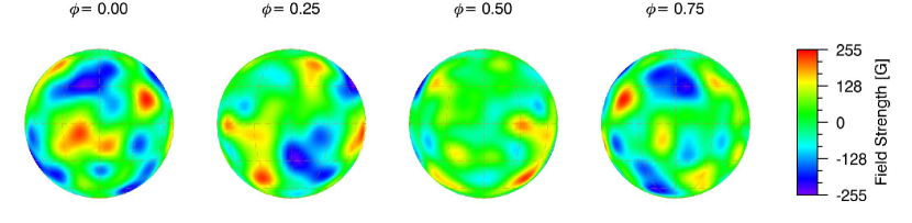
Figure 1: Orthographic maps of the random magnetic distribution of the test star at four different rotational phases $\phi$.

Before we address the problem of estimating the noise level on each resolution scale $j$, we take a closer look at the detection problem. The wavelet transform yields a level- or resolution-dependent representation of the observed spectral line profile in terms of the wavelet coefficients $w_{j,k}$. A decision about whether this wavelet coefficient is significant, i.e., whether it includes signal information or not, can be cast in a hypothesis-testing framework. For this, we can state the null hypothesis $H_{0}$ such that $w_{j,k}$ contains only noise and no signal information. Whether the null hypothesis will be rejected or not depends on probability $P_{n}$,

$$P_{n}\>=\>Prob(\|w_{j,k}\|<\tau|H_{0})\>,$$ (44)

where $\tau$ is a detection threshold. The null hypothesis will be rejected if $P_{n}$ is smaller than a given significance level $\epsilon$; i.e. $P_{n}(\tau)<\epsilon$ . For a Gaussian noise distribution with zero mean and standard deviation $\sigma$, we may write the probability density for $w_{j,k}$ as

$$p(w_{j,k})\>=\>\frac{1}{\sqrt{2\pi}\sigma}\>e^{\frac{-w_{j,k}^{2}}{2\sigma^{2}_{j}}}\>.$$ (45)

The probability $P_{n}$ of rejecting $H_{0}$ can then be calculated by integrating over all weights $w_{j,k}$ that are greater than a threshold $\tau$,

$$P_{n}^{+}\>=\>\frac{1}{\sqrt{2\pi}\sigma}\>\int_{\tau}^{+\infty}\>e^{\frac{-w_{j,k}^{2}}{2\sigma^{2}_{j}}}\>dw_{j,k}\>.$$ (46)

Since the wavelet transform of the Stokes profile can have both positive and negative values, we also need to integrate over all negative weights $w_{j,k}$ up to the threshold value $-\tau$

$$P_{n}^{-}\>=\>\frac{1}{\sqrt{2\pi}\sigma}\>\int^{-\tau}_{-\infty}\>e^{\frac{-w_{j,k}^{2}}{2\sigma^{2}_{j}}}\>dw_{j,k}\>.$$ (47)

When assuming stationary noise and choosing a specific significance level $\epsilon$, this reduces to the following decision or threshold detection rule (e.g., Starck & Murtagh 2006)

$$\|w_{j,k}\|\>\geq k\sigma_{j}\>\mbox{then $w_{j,k}$ is significant}\hskip 19.91684pt$$

$$\|w_{j,k}\|\>\leq k\sigma_{j}\>\mbox{then $w_{j,k}$ is not significant}\>,$$ (48)

where $k$ depends on the value of $\epsilon$. Choosing $\epsilon=0.0027$ results in $k=3,$ the well known $3\sigma$ detection threshold. This thresholding detection scheme can be introduced readily into the OMP algorithm of Sect. 3.1 by implementing the threshold detection rule of Eq. (48) as an additional step (Ib) after calculating the maximum projection (i.e. inner product) in step (I). If the currently selected wavelet coefficient is not significant, it will be deleted from the dictionary for this iteration cycle, and the algorithm restarts the current iteration cycle with step (I). The noise level $\sigma_{j}$ for each scale $j$ can be obtained by a wavelet transform of simulated noise. This process yields level-dependent thresholds and has the advantage that different types of noise (e.g., Gaussian or Poisson), as well as correlated noise, can be modeled.

4 Application to synthetic observations

We now use the OMP algorithm to estimate the effective and apparent longitudinal magnetic field. Before we begin with a statistical analysis of the accuracy of our proposed method, we give an illustrative example to highlight the functionality of the algorithm. The decomposition of an observed Stokes $V$ profile into the building blocks of the wavelet dictionary provides the opportunity for each selected signal or profile atom to be individually analyzed in terms of the effective and apparent longitudinal magnetic field. Thanks to the linearity of the algorithm, we can evaluate Eqs. (17) and Eq. (23) for each signal atom and iteratively approximate the desired magnetic quantities. Each contributing signal atom found by the OMP algorithm identifies a resolved structure in the wavelength (or velocity) domain. The overall number of iterations then also determines the summation index $n$ for the apparent longitudinal field in Eq. (23). The stopping criterion is given by the detection threshold as soon as the approximation enters the noise and no more significant signal atoms are detected.

In the following example we have built a stellar surface model with our iMap code (Carroll et al. 2012). We created a random distribution of a radial magnetic field; i.e., each surface segment has a Gaussian random distribution of its radial magnetic field strength with a mean value centered at zero Gauss and a standard deviation of 500 Gauss. The effective temperature of the test star is 5250 K, and it has solar abundance and a gravity of log$(g)=4.0$. The projected rotational velocity $v\sin i$ is $35$ km s^-1, and micro- and macroturbulence were set to 2 km s^-1. The inclination of the rotational axis is 90^∘. Because the original surface-grid resolution with a 5^∘ by 5^∘ segmentation creates a strong cancellation of the Stokes $V$ signal we decided, for this example case, to additionally smear out the distribution over the surface with a Gaussian filter that has an angular spread of 15^∘.

This smoothing leads to large random clusters of magnetic fields over the surface. The resulting magnetic field surface distribution is shown in Fig. 1. For the synthetic calculation, we used the magnetically sensitive iron line at 6173 $\AA$. Line parameters were taken from the VALD line database (Piskunov et al. 1995; Kupka et al. 1999). The resulting synthetic Stokes $V$ profile for phase 0.0 is shown in Fig. 2.

Figure 2: Stokes $V$ of the Zeeman sensitive iron line FeI 6173 for the random field distribution of the test star at phase 0.0.

To highlight the performance of the method, we used noise-free Stokes profiles in this first test. The stopping criterion for the noise-free case was substituted by a convergence criterion where the iteration was stopped as soon as there was no significant improvement in the root-mean-squared (RMS) error of the approximation. The approximations are illustrated in Fig. 3 where four snapshots at different stages in the approximation process are shown.

Figure 3: Magnetic OMP approximation at different iteration cycles. The true synthetic profile (solid line) and the approximation of the OMP method (dashed line).

The magnetic OMP algorithm gradually identifies the most coherent signal atoms on different scales and positions before it finally approximates the entire observed Stokes $V$ profile with a linear combination of all selected dictionary atoms. As can be seen in Fig. 3, the algorithm finds the one best-matching signal atom in the first iteration (upper left). In the approximations 5 (upper right), 10 (lower left), and 20 (lower right) one can follow the rapid improvement after adding more and more signal atoms to the residuals. Already at iteration cycle 10 (i.e., 10 dictionary atoms), the differences between the original synthetic observation and the approximation is hardly visible. In Fig. 4 the RMS error of the approximation is plotted over the iteration cycle, which also demonstrates the rapid convergence of the magnetic OMP algorithm. However, the approximation of the pure Stokes $V$ profile is not the main task of the magnetic OMP method here, because it is supposed to give accurate estimates of the effective and apparent magnetic field as well.

The effective and apparent longitudinal magnetic field is estimated during the approximation process from each contributing signal atom. To compare the estimated values with the true values, we need to extract the true effective longitudinal magnetic field from the model star. This is straightforward and only requires projecting the magnetic field vector of each surface segment onto the line-of-sight and eventually to sum the area-weighted contribution up from all visible surface segments. The extraction of the true apparent longitudinal magnetic field value from the model deserves some more explanation. In principle we could use the same process as for the effective longitudinal field and sum the absolute value up instead of the plain values from the stellar model, but this would not take the cancellation of the Stokes $V$ signals coming from within iso-radial velocity strips into account. We would therefore overestimate the apparent field; in fact, we would retrieve the total absolute effective longitudinal magnetic field. To obtain an adequate value for the apparent longitudinal magnetic field, we need to bring the surface distribution of the longitudinal magnetic-flux density into an appropriate iso-radial velocity binning before we can add up their absolute contributions.

Table 1: Parameter ranges used for the model atmosphere and synthetic line calculations.

Lower value	Parameter	Upper value
4500 K	$T_{\rm{eff}}$	6500 K
-2.0	$[M/H]$	+0.2
2.0	$\log g$	4.5
20 km/s	v$\sin$$i$	75 km/s

The resolution of this iso-radial velocity binning depends on the width of the used (local) spectral line; i.e., the broader the spectral line, the less surface flux can be deduced, and vice versa. Therefore we first translate the surface distribution of the longitudinal field of the model star onto a fine-binned rotational velocity coordinate axis. The resolution of this one-dimensional coordinate axis has the same resolution as our synthetic spectral line profile, i.e. 0.5 km s^-1. The distribution of the longitudinal magnetic flux density along the rotation velocity is then convolved with an area-normalized local Stokes $I$ profile to obtain the measurable longitudinal flux-density spectrogram over the rotational velocity which is depicted in Fig. 5.

We then sum over the absolute values of the longitudinal flux-density spectrogram to finally obtain the apparent longitudinal magnetic field that is compared to the estimates of the OMP method. In our test case (phase=0.0), the true effective longitudinal magnetic field inferred from the model is 4.67 Gauss and the apparent longitudinal magnetic field is 16.43 Gauss. From the magnetic OMP algorithm, we obtain a value of 4.53 Gauss for the effective longitudinal magnetic field and 16.78 for the apparent longitudinal magnetic field. An exhaustive statistical evaluation is given in the next section, but one can already see that besides the good approximation and the rapid convergence, the method also yields accurate values for both magnetic quantities.

Figure 4: The root mean square approximation error over the iteration cycle.

There is another interesting effect that highlights the complementary nature of the effective and apparent longitudinal magnetic field. At phase 0.25 of our test star, the polarities in the longitudinal magnetic field are almost perfectly balanced over the visible hemisphere. The resulting profile (again synthesized for the iron line FeI 6173) is shown in Fig. 6. The almost perfect balancing of polarities is not obvious from the line profile itself. However, if we estimate the longitudinal magnetic field by the COG method’s Eq. (16) and the magnetic OMP algorithm, we obtain 0.005 G or 0.007 G, respectively, for the effective longitudinal magnetic field.

We thus have an extremely small longitudinal magnetic field or none at all. This is not what one would expect from the mere visual inspection of the Stokes $V$ profile in Fig. 6, which apparently shows a clear net absolute polarization. In fact, the amplitude of the Stokes $V$ signal is even greater than the one of phase=0.0, shown in Fig. 2. This demonstrates the strength of the definition of the apparent longitudinal magnetic field; the magnetic OMP algorithm detects a clear apparent longitudinal field of 18.63 G (true value 17.98 G), which is slightly stronger even than in phase 0.0. The quantity of the apparent magnetic longitudinal field is therefore of particular interest in cases where balanced field distributions cause the first-order moment of the Stokes $V$ profile to vanish.

Figure 5: Distribution of the longitudinal magnetic flux density across the rotational velocity for phase 0.0 of the test star.

Figure 6: Stokes $V$ profile of the Zeeman sensitive iron line FeI 6173 for the random distribution at phase 0.25 of the test star.

Figure 7: The mean relative approximation error for the OMP dictionary and the PCA expansion. The relative error of the approximation is plotted over the number of signal atom (eigenprofiles for the PCA). The error declines steeply for both expansion methods; however, the OMP expansion shows a better performance, i.e., sparsity behavior compared to the PCA.

5 Numerical experiments and statistical evaluation

In this section we assess the accuracy of the OMP algorithm under a broad range of model conditions and for different spectral lines. For that reason we synthesized a large number of Stokes $I$ and Stokes $V$ profiles for different magnetic surface distributions and atmospheric conditions. The model parameters are the effective temperature, metallicity, surface gravity, projected rotational velocity, and the surface magnetic field and its distribution. For each set of the atmospheric parameters, we created a random surface distribution in the same way as for the previous example in Fig. 1. The atmospheric parameters were randomly chosen from within an interval given in Table 1. For the model atmospheres, we chose Kurucz/Atlas-9 models (Castelli & Kurucz 2004).

Figure 8: Error distribution of the longitudinal magnetic field calculated from 15,000 synthetic Stokes profiles by the magnetic OMP method (left) and the center-of-gravity (COG) method (right). Both methods show very good accuracy with a mean absolute percentage error of 1.87 % (magnetic OMP) and 1.79 % (COG).

Because the model atmospheres are provided on a fixed grid of step sizes of 250 K for the effective temperature, 0.5 for the logarithmic abundance and gravity, the atmospheres are interpolated for each randomly chosen set of atmospheric parameters. As Zeeman-sensitive spectral lines we chose three magnetically sensitive lines; the iron lines FeI 5497 ($g_{\rm eff}=2.22$), FeI 6173 ($g_{\rm eff}=2.50$), and FeI 8468 ($g_{eff}=2.50$). All line parameters were again taken from the VALD line database (Piskunov et al. 1995; Kupka et al. 1999). For each spectral line, we created a sample of 5,000 randomly chosen atmospheric parameters, rotational velocities, and magnetic surface distributions to eventually synthesize a set of corresponding Stokes $I$ and Stokes $V$ profiles with the forward module of our iMap code.

In total, we calculated a set of 15,000 Stokes $I$ and Stokes $V$ profile, which were then analyzed by our magnetic OMP algorithm. The true effective longitudinal magnetic field is directly extracted from the magnetic surface distribution of the synthetic model star. The true apparent longitudinal magnetic field is obtained from the convolved magnetic spectrograms as described above. Because the individual trials, sets of atmospheric parameters, and surface magnetic field values have different scales, we chose a relative performance metric to describe the accuracy.

The overall performance is judged by the mean absolute percentage error, while for illustrating the error distribution we use the relative percentage error. The relative percentage error is defined as

$$D_{i}\>=\>\frac{B^{T}_{i}-B^{OMP}_{i}}{B^{T}_{i}}\>*\>100\>,$$ (49)

where $B^{T}_{i}$ is the true magnetic field, and $B^{OMP}_{i}$ the calculated magnetic field of the $i$-th sample. Finally, the mean absolute percentage error (MAPE) is defined by

$$M_{B}\>=\>\frac{1}{n}\>\sum_{i=1}^{n}\>\left|D_{i}\right|\>.$$ (50)

5.1 Sparsity of Stokes profiles

Before we evaluate the performance of the OMP algorithm, we look more closely at the general sparsity of Stokes profiles. A sparse representation is often achieved by transforming a vector from the original data domain into a domain where the transformed coefficients (i.e., expansion coefficients) allow a more compact representation of the information (e.g., Fourier or wavelet transform). A vector is called sparse if there is a representation where most of the vector entries are zero or close to zero. A sparse approximation is performed by restricting the sparse transformation to the largest expansion coefficients such that there is no great loss of signal information.

Recently, Asensio Ramos & Lopez Ariste (2010) have shown that Stokes profiles are sparse and compressible under various transformations (e.g., wavelets and empirical basis functions). Compressible here means that the values of the sorted expansion coefficients exhibit an exponential decay that in turn results in a small approximation error (Candes & Wakin 2008). Although we saw from the numerical simulation of the last section that a sparse representation of a synthetic Stokes profile is possible with our dictionary elements, we also want to test empirically if this also holds for the entire set of our 15,000 Stokes profiles. To quantify the approximation error, we use the relative error, $\sum_{i}^{n}\frac{1}{n}\frac{\|\hat{\@vec{S}}_{i}-\@vec{S}^{*}_{i}\|}{\|\@vec{S}^{*}_{i}\|}$ where $\hat{\@vec{S}}$ is the approximation and $\@vec{S}^{*}$ the original Stokes vector.

To compare the performance of the OMP expansion relative to a known sparse decomposition, we also calculated a principal component analysis (PCA) of the entire synthetic data set. A PCA decomposes a set of observed Stokes profiles into an empirical set of orthogonal eigenprofiles (e.g., Carroll et al. 2008). As has been shown by Asensio Ramos & Lopez Ariste (2010) and Asensio Ramos & Allende Prieto (2010), a PCA expansion can result in a compact and sparse representation of Stokes profiles. Figure 7 shows how the dictionary used with the OMP algorithm performs against a PCA decomposition of our synthetic data set. Both curves (solid OMP, dashed PCA) show a rapid decline of the mean approximation error with increasing numbers of signal atoms or eigenvectors, respectively.

Figure 9: Error distribution of the apparent longitudinal magnetic field calculated by the magnetic OMP method. The mean absolute percentage error from the entire set of 15,000 synthetic test calculations is 4.67 %.

The performance of our dictionary of Gaussian derivatives is better than that of the empirical basis functions (i.e., eigenprofiles) obtained by the PCA. The reason for that is two-fold: First, the signal atoms of our dictionary are selected a priori to match the building blocks (i.e., elementary waveforms) of our problem and second the redundancy of our dictionary facilitates a more efficient expansion then that of the orthogonal eigenvectors of the PCA.

In contrast to the empirical basis formed by the PCA, the OMP dictionary is not required to be a set of orthogonal basis functions, and this generally provides better flexibility and adaptivity to approximate a given signal (Candes & Wakin 2008).

To reduce the relative approximation error with the OMP algorithm below 5%, it takes on average only nine signal atoms. Using 22 signal atoms the relative error is on average smaller than 1 %, which demonstrates that our dictionary allows a sparse representation of Stokes profiles for the parameter regime given in Table 1.

Figure 10: Mean absolute percentage error (MAPE) of the effective longitudinal magnetic field calculated over the relative noise level for the COG method (open circles) and the magnetic OMP method (solid circles).

Figure 11: Mean absolute percentage error (MAPE) of the apparent longitudinal magnetic field calculated versus the relative noise level.

Figure 12: A noiseless (noise level 0.0) example profile (solid line), and its OMP approximation (dashed line).

5.2 The noise-free case

To obtain an idea about the principal accuracy of the magnetic OMP algorithm and its performance relative to the conventional COG method, we began with a noise-free test case where the entire test sample of 15,000 Stokes $I,$ and Stokes $V$ profiles were used without any noise contribution.

In this simulation the overall error value for the effective longitudinal magnetic field obtained from the magnetic OMP algorithm yielded a MAPE of 1.87 %. For comparison the effective longitudinal magnetic field calculated by the COG method shows a similar MAPE of 1.79 %. The same error for the apparent longitudinal magnetic field is 4.67 %. The error for the three individual spectral lines show no apparent deviation from the overall error.

For the subset of synthetic Stokes $V$ profiles of the FeI 5497, we obtain a MAPE for the effective (apparent) longitudinal magnetic field of 1.80 % (4.57 %), for the FeI 6173 lines a MAPE of 1.93 % (4.69 %), and for the FeI 8468 lines a MAPE of 1.88 % (4.72 %). The error distribution for the relative percentage error of the effective longitudinal field calculated by the OMP and the COG method is shown in Fig. 8. Both the OMP method and the conventional COG method provide equally good results. The error distribution of the apparent longitudinal magnetic field is shown in Fig. 9. Given that the apparent field is even harder to determine due to possible cancellation effects of the Stokes $V$ signals, the error is still remarkably low, and the OMP method is able to recover the apparent field from the Stokes $V$ profiles with good accuracy.

5.3 The noise case

In the following we test the accuracy of the magnetic OMP method and the COG method for the more relevant case when the Stokes $V$ profiles are contaminated with noise. For that reason we have added an increasing amount of white noise to the 15,000 Stokes $V$ profiles. Since the Stokes $V$ profiles generated from the random surface distribution are of different magnitudes, we define a relative noise level $\eta$ that is given by the relative variance of the Stokes $V$ profile and that of the noise according to

$$\eta_{\rm rel}\>=\>\frac{\sigma(N)}{\sigma(S)}\>,$$ (51)

where $\sigma(S)$ and $\sigma(N)$ are the standard deviations of the Stokes $V$ profile and the noise contribution, respectively. Figure 10 shows how the relative error increases with higher noise levels. It is interesting how rapidly the accuracy of the COG method deteriorates (upper curve) compared to the relative robustness of the magnetic OMP method (lower curve). Already for a noise level of $\eta_{\rm rel}$ = 0.3, the accuracy of the COG method is significantly affected, whereas the OMP method still provides good accuracy with errors of less than 10 %. Even for a noise level of unity, the OMP method has an error of just 18 % where the COG method with an error of almost 50 % can no longer be considered a meaningful tool for quantifying the magnetic field. For the apparent longitudinal magnetic field, the OMP method shows a very robust performance as well. The error distribution over the relative noise level is illustrated in Fig. 11. The good performance and robustness of the magnetic OMP method compared to the COG method can be understood by considering the noise-free Stokes $V$ profile in Fig. 11. Because the OMP algorithm gradually approximates the noisy profile with a linear combination of dictionary profile atoms, it calculates the effective and apparent longitudinal magnetic field for each of the selected profile atoms separately. The detection mechanisms of Sect.3.3 prevent the algorithm from approximating insignificant profile features and thus largely avoids the quantification of the contributing noise.

Figure 13: Magnetic OMP approximations (dashed lines) to a noisy Stokes $V$ profile (solid lines) for different relative noise levels. Despite the increasing relative noise, the OMP approximation identifies the main characteristic and shape of the underlying noise-free profile.

Figure 12 shows one of the sample profiles generated for a random surface distribution of the magnetic field. The noiseless profile is approximated well by the OMP method, and the estimated effective and apparent longitudinal magnetic field is approximated with –41.04 G and 59.88 G, respectively, which is very close to the true values of –40.11 G and 61.65 G. The noiseless profile is approximated by the maximum number of 40 iterations, which means that 40 dictionary profile atoms are used to approximate the example profile. However, already the first three profile atoms are able to approximate the profile to such a degree that 95 % of the signal variance are described. In Fig. 13 the same profile can be seen with varying degrees of noise contributions overplotted again by the approximation from the OMP algorithm. Despite the increasing relative noise level, the OMP algorithm finds a good approximation to the original Stokes $V$ profile. The iteration for a noise level of $\eta_{\rm rel}$ = 0.25 stops already at seven iterations (i.e., 7 profile atoms). For $\eta_{\rm rel}$ = 0.5, 0.75, and 1.0, the iteration is stopped at cycles 6, 4, and 3, respectively. At a relative noise level of unity only three signal atoms are used to approximate the Stokes $V$ profile. However, as one can see from the noiseless case, these three signal atoms already capture the essential profile shape and amplitude of the original Stokes $V$ signal. Since the magnetic OMP algorithm interprets and analyzes each signal atom separately, the good approximation directly translates to a good estimates of the underlying effective and apparent longitudinal magnetic field. In this particular case, the estimations for the effective (apparent) longitudinal field from the magnetic OMP algorithm is –42.54 G (64.27 G) for a noise level of 0.25, –44.26 G (65.71 G) for a noise level 0.5, –36.04 G (68.85 G) for a noise level 0.75, and –34.77 G (72.54 G) for noise level of 1.0.

5.4 Absolute limits of the COG and OMP method

Until now we have analyzed the performance of the magnetic OMP and COG method by using relative noise levels. To shed more light on the absolute performance limits of the two methods, we take a closer look on the absolute values of the noise. Multiline reconstruction techniques like LSD (Donati et al. 1997) or SVD (Carroll et al. 2012) allow us to drastically lower the noise levels of spectropolarimetric observations. The thus increased signal-to-noise (S/N) levels allows detecting faint signal profiles that were otherwise deeply buried in the noise.

A natural question that arises in the context of magnetic field estimation is how much of the residual noise is falsely interpreted as magnetic field and up to which limits we can reliably estimate a true underlying magnetic field. To address this problem, we could simply perform a first-order perturbation to the COG method and apply standard error propagation to estimate the influence of the noise. However, for weak magnetic fields, the noise contribution relative to the true signal amplitude is in general not small anymore. We therefore simulate the process with a large and statistically significant number of synthetic profiles to determine the impact of typical absolute noise levels on the magnetic field estimation.

We assume additive Gaussian noise with zero mean. One might expect that this would lead to a vanishing value in the field estimation by the COG method. This is, however, not true for a finite spectral resolution. The random fluctuations and the unequal weighting in the velocity (or wavelength) domain can lead to relatively large spurious contributions to the first-order moment, hence to the field estimation as shown in the following simulation. Note that any form of correlated noise would even exacerbate the problem since it would introduce a systematic bias in the evaluation of the first-order moment.

With our assumption of white noise, a Stokes $\tilde{V}^{*}$ profile can be written as the sum of the true noiseless Stokes $\tilde{V}$ profile and a noise vector $N$,

$$\tilde{V}^{*}(\textrm{{v}})\>=\>\tilde{V}(\textrm{{v}})\>+\>N(\textrm{{v}})\>.$$ (52)

The effective or mean longitudinal field as measured by the COG method can then be written as

$$B_{\rm eff}=\frac{\lambda_{0}\>\int_{V}\left(\tilde{V}(\textrm{{v}})+N(\textrm{{v}})\right)\>\textrm{{v}}\>d\textrm{{v}}}{c\>\alpha\>W_{I}}\>.$$ (53)

We assume that the noise level is small enough that the estimation of the Stokes $I$ equivalent width remains largely unaffected.

The first-order moment of a noisy Stokes $\tilde{V}^{*}$ profile, as well as the magnetic field estimation, can then be split into a signal ($B^{S}_{\rm eff}$) and a noise ($B^{N}_{\rm eff}$) contributing part,

$$B_{\rm eff}\>=\>B^{S}_{\rm eff}\>+\>B^{N}_{\rm eff}\>=\>\frac{\lambda_{0}}{c\>\alpha\>W_{I}}\>\left(\int_{V}\tilde{V}(\textrm{{v}})\>\textrm{{v}}\>d\textrm{{v}}+\int_{V}N(\textrm{{v}})\>\textrm{{v}}\>d\textrm{{v}}\right)\>.$$ (54)

Written in this form we may ask to which noise level the following relation is valid, $B^{S}_{\rm eff}>B^{N}_{\rm eff}$, or at which point does a noise-induced magnetic field interfere with the magnetic field estimation from the true signal profile.

For the simulations we defined the absolute noise level $\eta_{abs}$ as the standard noise deviation $\sigma_{N}$ relative to the continuum of the normalized intensity profile, i.e., $\eta_{\rm abs}=\sigma_{N},$ which is also commonly used to describe the S/N level ($1/\sigma_{N}$) in stellar polarimetry (Donati et al. 1997). To mimic a multiline, reconstructed line profile (e.g., LSD profile), we created a fictitious iron line with a mean Landé factor of 1.2 at a rest wavelength of 5000 Å. The oscillator strength and van der Waals damping were adjusted to give an equivalent width for the Stokes $I$ profile of 100 mÅ. The Stokes $I$ and Stokes $V$ noise profiles were calculated with a resolution of $\lambda/\Delta\lambda=$100,000, which is common to current high-resolution observations. The spectral range covers a velocity of plus/minus 50 km s^-1 around the line center, and integration limits were set accordingly.

We chose noise levels from 10^-3 down to 10^-5 that correspond to a polarimetric sensitivity of 0.001 %, a level that is reached by current reconstruction methods (Donati & Landstreet 2009). We selected 20 noise levels between 10^-5 and 10^-3, equally spaced on a logarithmic scale. For each absolute noise level, we synthesized 10 000 noisy line profiles such that we have a total set of 200 000 simulated profiles.

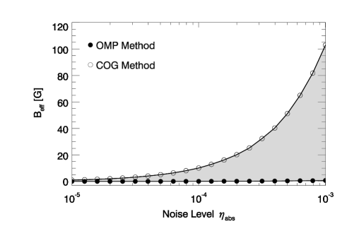
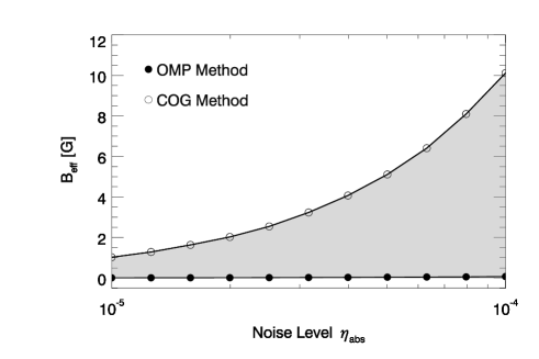
Figure 14: The effective magnetic field response over the absolute noise level (logarithmic scale) for the COG method (open circles) and the OMP method (solid circles). The response curve shows how much of the noise is erroneously attributed to a magnetic field. On the left side, the response is shown for a noise range between 10^-5 and 10^-3. The noise response of the COG method rapidly increases with the noise level from 2 to 100 G, whereas the OMP method remains largely unaffected by the noise with a flat response not larger than 0.7 G. On the right side, a close-up of the magnetic response curve for the region between 10^-5 to 10^-4 is shown. Even in such a low noise regime, the COG method falsely interprets a significant portion of the noise as magnetic field. The OMP method stays essentially flat at a level close to zero over the entire region. The gray shaded area marks the region of incorrect response for the COG method, i.e. $B^{S}_{\rm eff}<B^{N}_{\rm eff}$, and defines the lower limit for magnetic field detections

Owing to the linear superposition of the signal and noise contribution in Eq. (54), we do not depend on an underlying magnetic field and only need to simulate, besides the Stokes $I$ profile, the noise part of the profile. To quantify the magnetic response to the noise, we calculated the effective longitudinal magnetic field for each synthetic noise profile with the COG and the OMP methods. To obtain a statistical meaningful average response for each of 20 noise levels, we computed the mean of the absolute effective field from each of the corresponding 10 000 field values.

In Fig. 14, we plotted the magnetic response of the COG and of the OMP method over the various noise levels. From the response curve, we can immediately identify how much of the noise is falsely interpreted as a magnetic field. As the noise level increases, the COG method is increasingly affected by the noise, and more and more of the content of each noise profile is interpreted as an effective longitudinal magnetic field. For the COG method, a noise level of 10^-3 results, on average, in an effective longitudinal magnetic field of 101 G. On the right side of Fig. 14, we expand the region between 10^-5 to 10^-4. A few times 10^-5 is the region where many of the recently detected weak magnetic fields are reported (e.g., Aurière et al. 2009; Lignières et al. 2009; Aurière et al. 2010; Grunhut et al. 2010; Konstantinova-Antova et al. 2010; Petit et al. 2011; Fossati et al. 2013). Despite the low noise level, we see that the COG method interprets a non-negligible amount of the noise as a magnetic field (between 2 and 10 G).

The shaded areas in Fig. 14 mark the region of magnetic field values that can no longer be properly interpreted by the COG method, i.e., the region where $B^{S}_{\rm eff}<B^{N}_{\rm eff}$. In that sense the response curves set the lower limit or a noise threshold for the estimation of weak magnetic fields. However, even when the true field strength is above these threshold values, the relative contribution from the noise can severely compromise the field estimation of the COG method as was shown in Sect.5.3. For the magnetic OMP method, on the other hand, we see from Fig. 14 that the response is largely flat.

The magnetic field estimation from the OMP method is almost unaffected by the noise and shows only a small increase with the noise level. The incorrectly attributed field values are no higher than 0.7 G. This has its origin in the multiresolution thresholding scheme implemented in the OMP algorithm (see Sect.3.3).

Only those signal or noise features that reach a certain significance are interpreted and quantified. This again results in the good performance and robustness against the contributing noise. A dark gray area that shows the incorrect response region of the OMP method is not visible in Fig. 14 due to the low noise response of the OMP method. The specific values for the noise response of the COG method also depend of course on the line parameters, such as wavelength, equivalent width, and Landé factor. However, the deviations from our results are expected to be small because the spread in the derived average parameters for multiline reconstruction techniques that use line lists of many hundreds or thousands of lines are relatively small. The spectral resolution is also a contributing factor to the error of the COG method since the statistical fluctuations that enter into the evaluation of the first-order moment directly depend on the number of available wavelength points, such that lower spectral resolutions on average lead to larger errors (i.e., to a stronger noise response). However, a simulation and critical assessment of all these contributing factors in the COG estimation, are not subjects of the current paper.

6 Summary

This work presents a novel technique for detecting and quantifying stellar magnetic fields. By employing a sparse profile approximation in terms of an orthogonal matching pursuit algorithm, we were able to provide a robust method for detecting and estimating the effective longitudinal magnetic field.

By introducing the concept of the apparent longitudinal magnetic field, which describes the maximum of the resolvable absolute longitudinal surface field over the stellar disk, we provided a complementary measure to the effective or mean longitudinal magnetic field. For rapidly rotating stars, the definition of the apparent longitudinal magnetic field allows a quantification of the field even in situations where a small-scale and balanced surface field would otherwise result in a vanishing mean longitudinal magnetic field.

It was shown by an extensive numerical simulation with our iMap code (Carroll et al. 2012) that the accuracy of the OMP method is remarkably good with a mean absolute percentage error of only 1.87 % for the effective longitudinal magnetic field and 4.67 % for the apparent longitudinal magnetic field. However, the real strength of the new approach is its robustness against noise. Even for relative noise levels of unity, i.e., when the variance of the noise has the same magnitude as the actual Stokes $V$ signal, the OMP method has a mean error of only 18 %, whereas the conventional estimation by the COG method yields a mean error of almost 50 %.

In an effort to understand the limitations of the conventional COG method for estimating weak magnetic fields from faint and noisy Stokes $V$ signals, we simulated noise profiles in a low-noise regime from an absolute noise level of 10^-3 down to 10^-5. This is a regime that is currently reached by multiline reconstruction techniques such as LSD (Donati et al. 1997) or SVD (Carroll et al. 2012) and will be reached by the next generation of spectropolarimeters like PEPSI at the 2$\times$8.4m Large Binocular Telescope (LBT) (Strassmeier et al. 2008). In these low-noise regimes, however, a non-negligible fraction of the noise was incorrectly interpreted as a magnetic field by the COG method. Depending on the noise level, these falsely identified field values are between 2 and 100 G, making any attempt to estimate weak fields of a similar strength extremely difficult. The magnetic OMP method, on the other hand, again shows a remarkable robustness over the entire range of noise levels, where only 0.1 to 0.7 G are incorrectly attributed to a magnetic field. This makes the magnetic OMP method the method of choice for estimating weak magnetic fields from noisy Stokes profiles.

From a numerical perspective, the algorithm can be easily implemented and the iterative process is fast to evaluate. The magnetic OMP algorithm provides a viable tool for detecting and quantifying magnetic fields from spectropolarimetric observations. Although the focus in this work has been placed on disk-integrated Stokes profiles of stellar magnetic fields, this method is also directly applicable to resolved solar magnetic field observations.