Sensitivity of orbiting JEM-EUSO to large-scale cosmic-ray anisotropies

Abstract

The two main advantages of space-based observation of extreme-energy ($\gtrsim 10^{19}$ eV) cosmic-rays (EECRs) over ground-based observatories are the increased field of view, and the all-sky coverage with nearly uniform systematics of an orbiting observatory. The former guarantees increased statistics, whereas the latter enables a partitioning of the sky into spherical harmonics. We have begun an investigation, using the spherical harmonic technique, of the reach of JEM-EUSO into potential anisotropies in the extreme-energy cosmic-ray sky-map. The technique is explained here, and simulations are presented. The discovery of anisotropies would help to identify the long-sought origin of EECRs.

1 Introduction

The Extreme Universe Space Observatory (EUSO) is a consortium of 250 Ph.D. researchers from 27 institutions, spanning 14 countries. It is a down-looking telescope optimized for near-ultraviolet fluorescence produced by extended air showers in the atmosphere of the Earth. EUSO is proposed to occupy the Japanese Experiment Module (JEM) on the International Space Station (ISS), and collect up to 1000 cosmic ray (CR) events at and above 55 EeV ($1\,\rm{EeV}=10^{18}$ eV) over a $5$ year lifetime, far surpassing the reach of any ground-based project.

JEM-EUSO brings two new, major advantages to the search for the origins of EECRs. One advantage is the large field of view (FOV), attainable only with a space-based observatory. With a $60^{\circ}$ opening angle for the telescope, the down-pointing (“nadir”) FOV is

$$\pi(h_{\rm ISS}\tan(30^{\circ}))^{2}\approx h_{\rm ISS}^{2}\approx 150,000\,{\rm km}^{2}\,.$$ (1)

PAO has a FOV of 3,000 km². Thus the JEM-EUSO FOV, given in Eq. (1), is 50 times larger for instantaneous measurements (e.g., for observing transient sources). Multiplying the JEM-EUSO event rate by an expected 18% duty cycle, we arrive at a time-averaged nine-fold increase in acceptance for JEM-EUSO compared to PAO, at energies where the JEM-EUSO efficiency has peaked (at and above $\sim 100$ EeV). Tilting the telescope turns the circular FOV given in Eq. (1) into a larger elliptical FOV. The price paid for “tilt mode” is an increase in the threshold energy of the experiment.

The second advantage is the coverage of the full sky ($4\pi$ steradians) with nearly constant systematic errors on the energy and angle resolution, again attainable only with a space-based observatory. (Combined data from ground-based observatories in the Northern and Southern hemispheres may offer full-sky coverage, but not uniformity of systematics.) This talk pursues all-sky studies of possible spatial anisotropies. The reach benefits from the $4\pi$ sky coverage, but also from the increased statistics resulting from the greater FOV. A longer study will soon be completed and published [1].

In addition to the two advantages of space-based observation just listed, a third feature provided by a space-based mission may turn out to be significant. It is the increased acceptance for Earth-skimming neutrinos when the skimming chord transits ocean rather than land. On this latter topic, just one study has been published [2]. The study concludes that an order of magnitude larger acceptance results for Earth-skimming events transiting ocean compared to transiting land. Ground-based observatories will not realize this benefit, since they cannot view ocean chords.

2 All-sky coverage and anisotropy

As emphasized by Sommers over a dozen years ago [3], an all-sky survey offers a rigorous expansion in spherical harmonics, of the normalized spatial event distribution $I(\Omega)$, where $\Omega$ denotes the solid angle parameterized by the pair of latitude ($\theta$) and longitude ($\phi$) angles:

$$I(\Omega)\equiv\frac{N(\Omega)}{\int d\Omega\,N(\Omega)}=\sum_{\ell=0}^{\infty}\,\sum_{|m|\leq l}a_{\ell m}\,Y_{\ell m}(\Omega)\,,$$ (2)

i.e., the set $\{Y_{\ell m}\}$ is complete. Averaging the $a^{2}_{\ell m}$ over the $(2\ell+1)$ values of $m$ defines the rotationally-invariant “power spectrum” in the single variable $\ell$, $C(\ell)=\frac{1}{2\ell+1}\sum_{|m|\leq\ell}\,a^{2}_{\ell m}$. The set $\{Y_{\ell m}\}$ is also orthogonal, obeying

$$\int d\Omega\;Y_{{\ell_{1}}{m_{1}}}(\Omega)\,Y_{{\ell_{2}}{m_{2}}}(\Omega)=\delta_{{\ell_{1}}{\ell_{2}}}\,\delta_{{m_{1}}{m_{2}}}\,.$$ (3)

We are interested in the real valued $Y_{\ell m}$’s, defined as $P^{\ell}_{m}(x)(\sqrt{2}\cos(m\phi))$ for positive $m$, $P^{\ell}_{|m|}(x)(\sqrt{2}\sin(|m|\phi))$ for negative $m$, and $P_{\ell}(x)$ for $m=0$. Here, $P^{\ell}_{m}$ is the associated Legendre polynomial, $P_{\ell}=P^{\ell}_{m=0}$ is the regular Legendre polynomial, and $x\equiv\cos\theta$.

The lowest multipole is the $\ell=0$ monopole, equal to the average all-sky flux. The higher multipoles ($\ell\geq 1$) and their amplitudes $a_{\ell m}$ correspond to anisotropies. Guaranteed by the orthogonality of the $Y_{\ell m}$’s, the higher multipoles when integrated over the whole sky equate to zero.

A nonzero $m$ corresponds to $2\,|m|$ longitudinal “slices” ($|m|$ nodal meridians). There are $\ell+1-|m|$ latitudinal “zones” ($\ell-|m|$ nodal latitudes). In Figs. (1-3) we show the partitioning described by some low-multipole moments. The configurations with $(\ell,-|m|)$ are related to those with $(\ell,+|m|)$ by a longitudinal phase advance $\phi\rightarrow\phi+\frac{\pi}{2}$, or $\cos\phi\rightarrow\sin\phi$.

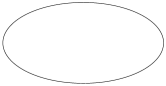
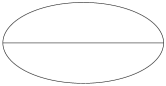
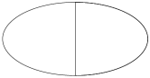
Figure 1: Nodal lines separating surplus and deficit regions of sky, for (left) $\ell=0,\ m=0$ monopole, and $\ell=1,\ m=0$ (middle) and $m=1$ (right) dipoles.

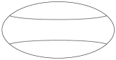
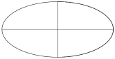
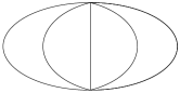
Figure 2: Nodal lines separating surplus/deficit regions of sky, for $\ell=2,\ m=0,\ 1,\ 2$ quadrupoles, respectively.

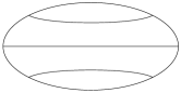
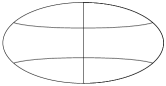
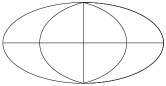
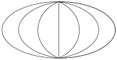
Figure 3: Nodal lines separating surplus/deficit regions of sky, for $\ell=3,\ m=0,\ 1,\ 2,\ 3$, respectively.

3 Previous anisotropy searches

The first full-sky large anisotropy search was based on the combined northern and southern hemisphere data from the SUGAR and AGASA experiments taken during a 10 yr period. Nearly uniform exposure to the entire sky resulted. No significant deviation from isotropy was seen, even at energies beyond $4\times 10^{19}$ eV [4]. More recently, the Pierre Auger Collaboration carried out various searches for large scale anisotropies in the distribution of arrival directions of cosmic rays above $10^{18}$ eV [5, 6].

The latest Auger study was performed as a function of both declination and right ascension in several energy ranges above $10^{18}$ eV, and reported in terms of dipole and quadrupole amplitudes. Again no significant deviation from isotropy was revealed. Assuming that any cosmic ray anisotropy is dominated by dipole and quadrupole moments in this energy range, the Pierre Auger Collaboration derived upper limits on their amplitudes. Such upper limits challenge an origin of cosmic rays above $10^{18}$ eV from non-transient galactic sources densely distributed in the galactic disk [7]. At the energies exceeding $6\times 10^{19}$ eV, however, hints for a dipole anisotropy may be emerging [8].

It must be emphasized that because previous data were so sparse at energies which will be accessible to JEM-EUSO, upper limits on anisotropy were necessarily restricted to energies below the threshold of JEM-EUSO. JEM-EUSO expects many more events at $\sim 10^{20}$ eV, allowing an enhanced anisotropy reach. In addition, JEM-EUSO events will have a higher rigidity ${\cal R}=E/Z$, and so will be less bent by magnetic fields; this may be helpful in identifying particular sources on the sky.

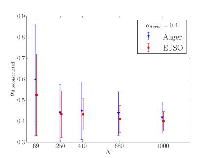
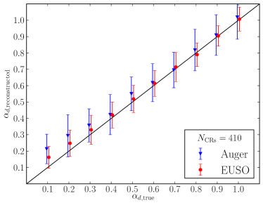
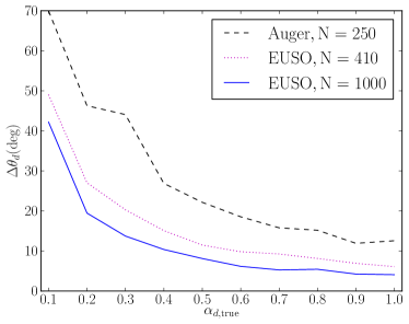
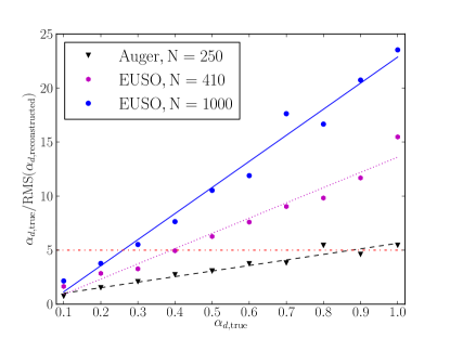
Figure 4: Reconstruction of the dipole amplitude (top panels) and angle (bottom-left panel), for PAO and JEM-EUSO. Discovery reach (bottom-right panel) of JEM-EUSO and PAO, with 5-$\sigma$ horizontal line.

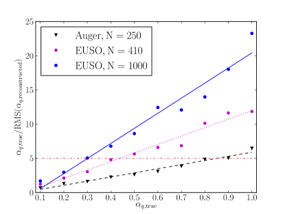
Figure 5: Discovery reach of JEM-EUSO and PAO with a 5-$\sigma$ horizontal line.

4 Comparison of all-sky JEM-EUSO to half-sky PAO

The ground-based Pierre Auger Observatory (PAO) is an excellent, ground-breaking experiment. However, in the natural progression of science, PAO will be superseded by space-based observatories. JEM-EUSO is designed to be first of its class, building on the successes of PAO.

The two main advantages of JEM-EUSO over PAO are the (i) greater FOV leading to a greater exposure at EE, and the (ii) all-sky nature of the orbiting, space-based observatory. We briefly explore the advantage of the enhanced exposure first. We consider data samples of 69, 250, 410, 680, and 1000 events. The 69 events sample is that presently published by PAO for events accumulated over three years at and above 55 EeV. The annual rate of such events at PAO is $\sim 69/3=23$. Thus, the 250 event sample is what PAO could attain in ten years of running.

Including the JEM-EUSO efficiency down to 55 EeV reduces the factor of 9 relative to PAO down to a factor $\sim$6 at and above 55 EeV. We arrive at the 410 event sample as the JEM-EUSO expectation at and above 55 EeV after three years running in nadir mode (or, as is under discussion, in tilt mode with an increased aperture but reduced PDM count). A 680 event sample is then expected for five years of JEM-EUSO in a combination of nadir and tilt mode. Finally, the event rate at an energy measured by High Resolution Fly’s Eye (HiRes) is known to exceed that of PAO by 50%. This leads to a five-year event rate at JEM-EUSO of about 1000 events.

Now we turn to the $4\pi$ advantage. Commonly, a major component of the anisotropy is defined via a max/min directional asymmetry, $\alpha\equiv\frac{I_{\max}-I_{\min}}{I_{\max}+I_{\min}}$. For a monopole plus dipole distribution $1+\alpha_{D}\cos\theta$, one readily finds that $\alpha=\alpha_{D}$. For a monopole plus quadrupole distribution $1-C\cos^{2}\theta$ (no dipole), one finds that $\alpha=\frac{C}{2-C}$, and $C=\frac{2\alpha}{1+\alpha}$.

In Fig. (4) we compare the capability of JEM-EUSO and PAO to reconstruct a dipole anisotropy. In this comparison, both advantages of JEM-EUSO, namely the increased FOV and the $4\pi$ sky coverage, are evident.

Dipole (plus monopole) plots are composed in the following way. First, we choose a dipole amplitude $\alpha_{\rm true}$ (relative to the monopole amplitude), and a dipole direction. The latter is randomly oriented, and defines the axis for the polar angle $\theta$. Then, a given number of events, 250, 410, or 1000, are randomly distributed within the weighting $1+\alpha_{\rm true}\cos\theta$. Next, the fitting algorithm determines, as best it can, reconstructed values for $\alpha$ and for the dipole direction. This process is repeated 100 times, each time with a different randomly oriented dipole direction. Results are averaged, and presented in the figures. This formulation results in our observation point, the Earth, being located at the center of the dipole distribution. A dipole distribution might be indicative of a single, dominant cosmic-ray source in the presence of a magnetic field.

In the top-left panel of Fig. (4) are shown the error bars that result from a reconstruction of the dipole amplitude (we have chosen $\alpha_{\rm true}=0.4$ for illustration), for the various $N$-event samples. The errors in $\Delta\alpha$ are seen to scale as $1/\sqrt{N}$ as one would expect for a Poisson distribution of events in $\cos\theta$. More significantly, the reconstruction errors in PAO for the dipole amplitude are almost twice those of JEM-EUSO, due to the limited sky-coverage of PAO (and even worse for the quadrupole, to be analyzed next) [9]. Moreover, if the dipole were aligned with the zenith angle of PAO, then PAO could easily confuse a quadrupole with a half-dipole. There is no such ambiguity with the $4\pi$ coverage of JEM-EUSO.

The top-right panel of Fig. (4) shows the error in reconstruction of the dipole amplitude, for a fixed event number $N=410$ events. Of course, PAO will not attain an event sample of 410, but the figure correctly displays the loss of quality when the acceptance is reduced from the all-sky $4\pi$ steradians to that of PAO, even for the same number of events as JEM-EUSO. The bottom-left panel of Fig. (4) shows the reconstruction errors on the dipole direction, versus the dipole amplitude, for three event samples, PAO with 250 events, and JEM-EUSO with 410 and 1000 events. Not surprisingly, the ability to reconstruct the dipole direction improves dramatically with an increase in the dipole amplitude. For $\alpha$ exceeding 0.2, the 410 event JEM-EUSO sample has less that half the error of the 250 event PAO sample, and the 1000 event sample has less than a third the error of the PAO sample.

The final panel in Fig. (4) gives the number of $\sigma$ for reconstruction of the dipole amplitude, as a function of the true dipole amplitude. The discriminatory power of $4\pi$ JEM-EUSO is obvious. A discovery claim (5-$\sigma$) is evident to PAO only for dipole amplitudes above 0.80. However, 410-event JEM-EUSO (3yrs) can claim discovery for an amplitude down to 0.40, and 1000-event JEM-EUSO can claim discovery all the way down to 0.28. The latter sample can reveal 3-$\sigma$ “evidence” for an nonzero dipole amplitude down to 0.20.

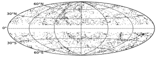
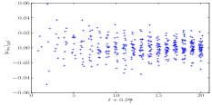
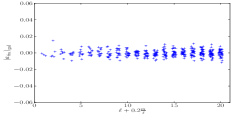
Figure 6: Sky-map of (left panel) the “5310 Galaxy-source” distribution, taken from the 2MRS catalog of galaxies [10] out to z=0.03 (115 Mpc), excluding the Galactic plane at $|b|\leq 10^{\circ}$; and the fitted $a_{\ell m}$ values (center panel). (right panel) $a_{\ell m}$’s from randomly distributed 5310-event “isotropic” data, excluding the same strip of Galactic plane. The $\ell/m$-dependency of the abscissa in the $a_{\ell m}$ plots is chosen [3] to increase the visibility of the $(2\ell+1)\ m$ values at fixed $\ell$. The $|b|\leq 10^{\circ}$ cut is accounted for analytically in each of the right two figures. Note the large $|a_{\ell=2}|$ values in the center figure.

In Fig. (5) we repeat the reconstruction comparison of JEM-EUSO and PAO, but this time for a quadrupole distribution. Our results are an average over 100 trials of a random but weighted distribution of a purely isotropic monopole and anisotropic quadrupole, the latter having a randomly chosen orientation, again with the Earth located at the center of the distribution. There is no dipole in the input data set. A quadrupole amplitude might be indicative of a dominant Galactic distribution of sources, or even of a distribution of dominant sources in the Supergalactic Plane. A general quadrupole ($\ell=2$) has five allowed $m$ values. Here we consider a pure $m=0$ distribution of events, i.e., a quadrupole with azimuthal symmetry about the quadrupole axis, as shown in the first sky-map of Fig. (2). We have again chosen $\alpha=0.4$ for illustration. The total distribution of events mimics an oblate spheroid with relative probability distribution $1-\frac{4}{7}\cos^{2}\theta$.

The same analysis as in Fig. (4) was done for the quadrupole case. A partial sky observatory fits a quadrupole much more poorly. Fig. (5) shows that JEM-EUSO can claim 5-$\sigma$ discovery of a quadrupole amplitude as low as 0.4 with 410 events, and as low as 0.3 with 1000 events. Also with 1000 events, JEM-EUSO is sensitive to a 3-$\sigma$ indication down to an amplitude of 0.2. On the other hand, PAO is incapable of claiming a quadrupole discovery unless the quadrupole amplitude is maximum, an unlikely value.

5 Future studies

In the near future, we will include several additional complicating, real world aspects of the spherical harmonic search for anisotropy. One relates to the energy resolution for individual events. With a spectrum falling steeply in energy, a spill-over of a lower-energy bin with isotropic events into a higher-energy bin with potentially anisotropic events will dilute the signal. While more study of this issue is warranted, this seems not to be a serious concern. PAO quotes an energy resolution $\Delta E/E$ of 22%, with 12% statistical, and about 20% systematic. Simulations in JEM-EUSO  to determine the energy resolution at extreme energies are ongoing, with the present upper limit $\sim 30\%$. Also, the data sample of JEM-EUSO used in anisotropy studies is not bound to the 55 EeV threshold that PAO chose due to its limited statistics. With more statistics expected, JEM-EUSO can choose a higher-energy threshold. Of course, any anisotropy will turn on gradually in energy, and simulations must include this fact.

Other probable non-concerns are the systematic error in the angular resolution of JEM-EUSO ($\lesssim 3^{\circ}$), and the bending of proton trajectories at extreme energies, given firstly by the random walk equation through extragalactic magnetic domains of strength $B_{\rm nG}$ in units of nanoGuass, and coherence size $\lambda$,

$$\delta\theta^{\circ}=0.8\,Z\,\left(\frac{B_{\rm nG}}{E_{20}}\right)\,\sqrt{\frac{D\,\lambda}{10\,{\rm Mpc}^{2}}}\,;$$ (4)

where Z and $E_{20}$ are the CR charge and energy in units of 100 EeV, respectively, and $D$ is the distance traveled by the CR. One sees that for a proton ($Z=1$) at 100 EeV, the natural unit of bending is a degree in the extragalactic magnetic field. On the other hand, heavy nuclei trajectories may be so severely bent as to eliminate even large-scale event anisotropies. So our hope hangs on protons being dominant at extreme energies. Complicating the issue is that the bending may be more or less if filamentary structure or voids are encountered en route. Subsequent to the transit of extragalactic space, the CR encounters the Galactic magnetic field, which is larger than than the extragalactic field, but is also known more precisely.

Our near-future studies will incorporate energy resolution effects, realistic estimates of Galactic and extragalactic magnetic fields, and “GZK” energy losses on cosmic radiation fields. To incorporate these effects, we will add energy and direction assignments for the individual simulated events in the context of two models, which we call the “Galaxy source model” and the “Single source model”, the latter being motivated by weak evidence for a UHECR excess in the direction of Centaurus A. For the Galaxy source model, the simulated source data is weighted to the 2MRS all-sky catalog of galaxies out to $z=0.03$ (about 115 Mpc) [10]. For the single source model, the simulated source data is fixed to a single source on the sky. For each data set, we will propagate the CRs to Earth and perform a multipole analysis of the resulting sky map.

The flavor of our work in progress can be gleaned from Fig. (6). The first panel in Fig. (6) presents the sky-map of the 5310 galaxies present in the 2MRS survey, which reaches out to z=0.03, corresponding to a distance $\sim z/H_{0}\sim 115$ Mpc. In the middle panel are shown the $a_{\ell m}$’s that result from the Galaxy-source model. As a control, the right panel displays the $a_{\ell m}$’s that result from an isotropic distribution of 5310 events with the same $y$ scale. In both analyses, the Galactic Plane at declination below $|b|\leq 10^{\circ}$ is omitted. An eyeball comparison of the two panels shows the power of the $a_{\ell m}$’s to reveal anisotropy. In particular we recover the predicted quadrupole structure in that the largest $|a_{\ell m}|$ are in the $\ell=2$ column.

6 Conclusions

The two main advantages of space-based observation of EECRs over ground-based observatories are increased FOV and $4\pi$ sky coverage with uniform systematics. The former guarantees increased statistics, whereas the latter enables a partitioning of the sky into spherical harmonics. We have begun an investigation, using the spherical harmonic technique, of the reach of JEM-EUSO  into potential anisotropies in the EECR sky-map. The discovery of anisotropies would help to identify the long-sought source(s) of EECRs.

This work is supported in part by a Vanderbilt Discovery Grant (TJW and PBD), NSF CAREER PHY-1053663 and NASA 11-APRA11-0058 Awards (LAA), Alfred P. Sloan Foundation (AAB), and NSF GAANN fellowship (MR).

References

References

- [1] Denton P B, Anchordoqui L A, Berlind A A, Richardson M and Weiler T J in progress
- [2] Palomares-Ruiz S, Irimia A and Weiler T J 2006 Phys.Rev. D73 083003 (Preprint astro-ph/0512231)
- [3] Sommers P 2001 Astropart.Phys. 14 271–286 (Preprint astro-ph/0004016)
- [4] Anchordoqui L A, Hojvat C, McCauley T P, Paul T C, Reucroft S et al. 2003 Phys.Rev. D68 083004 (Preprint astro-ph/0305158)
- [5] Abreu P et al. (Pierre Auger Collaboration) 2011 Astropart.Phys. 34 627–639 (Preprint 1103.2721)
- [6] Abreu P et al. (Pierre Auger Collaboration) 2012 Astrophys.J.Suppl. 203 34 (Preprint 1210.3736)
- [7] Abreu P et al. (Pierre Auger Collaboration) 2012 Astrophys.J. 762 L13 (Preprint 1212.3083)
- [8] Anchordoqui L A, Goldberg H and Weiler T J 2011 Phys.Rev. D84 067301 (Preprint 1103.0536)
- [9] There are some mathematical techniques that help PAO reconstruct, from partial sky coverage, any dipole anisotropy (see [11]). These techniques are ill-suited to quadrupole and higher multipoles.
- [10] Huchra J P, Macri L M, Masters K L, Jarrett T H, Berlind P et al. 2011 (Preprint 1108.0669)
- [11] Aublin J and Parizot E 2005 Astron.Astrophys. (Preprint astro-ph/0504575)