Spontaneous, collective coherence in driven, dissipative cavity arrays

Abstract

We study an array of dissipative tunnel-coupled cavities, each interacting with an incoherently pumped two-level emitter. For cavities in the lasing regime, we find correlations between the light fields of distant cavities, despite the dissipation and the incoherent nature of the pumping mechanism. These correlations decay exponentially with distance for arrays in any dimension but become increasingly long ranged with increasing photon tunneling between adjacent cavities. The interaction-dominated and the tunneling-dominated regimes show markedly different scaling of the correlation length which always remains finite due to the finite photon trapping time. We propose a series of observables to characterize the spontaneous build-up of collective coherence in the system.

Arrays of optical or microwave cavities, each interacting strongly with quantum emitters and mutually coupled via the exchange of photons, have been introduced as prototype setups for the study of quantum many-body physics of light Hartmann et al. (2006); Greentree et al. (2006); Angelakis et al. (2007). Even though ground or thermal equilibrium states of the corresponding quantum many-body systems are challenging to generate in experiments, much of the initial attention has focussed on this regime Hartmann et al. (2008); Tomadin and Fazio (2010); Houck et al. (2012); Carusotto and Ciuti (2013). In any realistic experiment with cavity arrays, however, photons are dissipated due to the imperfect confinement of the light, and emitter excitations have finite lifetimes. It is thus crucial and useful to explore the driven-dissipative regime of these structures, where photon losses are continuously compensated by pumping new photons into the cavities. A special role is here taken by the stationary states where photon pumping and losses balance each other in a dynamical equilibrium. This regime has thus received considerable attention in recent years, where coherent and strongly correlated phases have been discovered Carusotto et al. (2009); Hartmann (2010a); Nissen et al. (2012), but also analogies to quantum Hall physics Umucal ılar and Carusotto (2012) and topologically protected quantum states Bardyn and İmamoǧlu (2012) have been discussed.

In previous investigations of coupled cavity arrays in driven-dissipative regimes, the pump mechanism that injects photons into the array has been assumed to be a coherent drive at each cavity Carusotto et al. (2009); Hartmann (2010a); Nissen et al. (2012); Umucal ılar and Carusotto (2012); Bardyn and İmamoǧlu (2012). Therefore any phase-coherence between light fields in distant cavities that was seen in these studies can at least in part be attributed to the fixed phase relation between their coherent input drives. Here, in contrast, we show that such a coherence between distant cavities can build up spontaneously, triggered only by physical processes within the array. In this way we address the question of whether a non-equilibrium superfluid can develop in these structures. To this end, we consider a cavity array that is only driven by an incoherent pump which explicitly avoids any external source for a preferred phase relation between photons in different cavities.

In our model, each cavity strongly interacts with a two-level emitter. Whereas both, emitters and cavity photons, are subject to dissipation processes, the cavities are excited via the emitters only, which are population inverted by an incoherent pump. For a single cavity our model reduces to the previously considered and realized one-emitter laser Mu and Savage (1992); McKeever et al. (2003); Astafiev et al. (2007); Nomura et al. (2010); del Valle and Laussy (2011). Generalizations of this single cavity model have also been studied for two Yeoman and Meyer (1998) and multiple emitters Laussy et al. (2011); Auffèves et al. (2011); Poddubny et al. (2010) or emitters supporting multi-exciton states Gies et al. (2011).

We focus our analysis on the build-up of first-order coherence between the fields in distant cavities as this quantity is typically considered for investigating long range order and the emergence of superfluidity, e.g. in optical lattices Bloch et al. (2008). In cavity arrays these correlations can be measured by recording the interference pattern of the light fields emitted from the individual cavities. We find that collective correlations indeed build up in our set-up when the cavities are in the lasing regime. These correlations decay exponentially as the distance between the considered cavities tends to infinity for any dimension of the array. As intuitively expected, the associated correlation length increases with increasing photon tunneling between the cavities. For the interaction-dominated regime this increase is logarithmic, whereas it is a power law in the tunneling-dominated regime. Nonetheless, for any non-vanishing cavity decay rate, the correlation length always remains finite.

Related questions are of high relevance for ultra-cold atoms Diehl et al. (2008), ions Schindler et al. (2013) , superconducting circuits Marcos et al. (2012) or exciton-polariton condensates Carusotto and Ciuti (2013). For the latter, functional renormalization group approaches showed that, correlations at least decay exponentially in isotropic two-dimensional Altman et al. (2013) but can be long range in three-dimensional systems Sieberer et al. (2013).

Finally, we also find that the collective coherence build-up manifests strongly in the local cavity properties such as intensity and spectrum of emission. In particular, lasing and its typical photoluminescence (PL) lineshape, the Mollow triplet del Valle and Laussy (2010, 2011), can be observed far out of resonance between emitter and cavity as a result of the emergence of collective photonic modes.

Suitable experimental platforms for exploring our findings are superconducting circuit Houck et al. (2012), photonic crystal Majumdar et al. (2012); Rundquist et al. (2013), micro-pillar Abbarchi et al. (2013), or waveguide coupled cavities Lepert et al. (2011).

Model.—We consider an array of cavities, each of which interacts with a two level emitter, and is connected to adjacent cavities via photon tunneling. Our system, c.f. Fig. 1(a) and (b), is thus described by a Jaynes-Cummings-Hubbard Hamiltonian ($\hbar=1$),

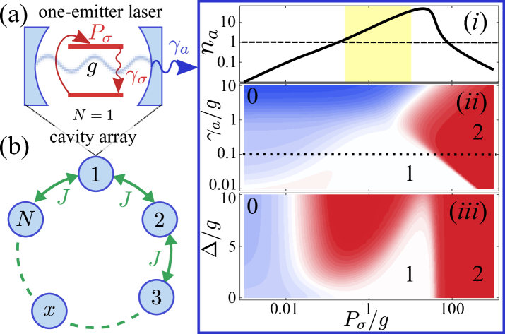
Figure 1: (Color online) (a) The building block of the array, the one-emitter laser and its main cavity emission properties: ($i$) cavity population $n_{a}$ as a function of $P_{\sigma}$ for $\gamma_{a}=0.1g$ and $\omega_{\sigma}=\omega_{a}$, with the lasing region highlighted in yellow. Below, contour plots of $g^{(2)}$ as a function of $P_{\sigma}$ and ($ii$) $\gamma_{a}$ at $\omega_{\sigma}=\omega_{a}$, or ($iii$) $\Delta=\omega_{\sigma}-\omega_{a}$ at $\gamma_{a}=0.1g$, with $g^{(2)}>1$ in red, $g^{(2)}=1$ in white and $g^{(2)}<1$ in blue. Also $\gamma_{\sigma}=0.01g$ and $J=0$. (b) Scheme of the total system in one dimension: a circular array of $N$ coupled cavities containing single emitters.

$$H=\sum_{j}H_{j}^{JC}+\sum_{<j,l>}J[{a_{j}^{\dagger}}a_{l}+{a_{l}^{\dagger}}a_{j}]$$ (1)

with $H_{j}^{JC}=\omega_{a}{a_{j}^{\dagger}}a_{j}+\omega_{\sigma}{\sigma_{j}^{\dagger}}\sigma_{j}+g({a_{j}^{\dagger}}\sigma_{j}+a_{j}{\sigma_{j}^{\dagger}})$, where $a_{j}$ is the photon annihilation operator and $\sigma_{j}=\left|\mathrm{g}\right\rangle_{j}\left\langle\mathrm{e}\right|_{j}$ the emitter de-excitation operator in cavity $j$. We assume periodic boundary conditions and a homogeneous array with photon tunneling rate $J$ so that all $H_{j}^{JC}$ feature the same photon frequency $\omega_{a}$, emitter transition frequency $\omega_{\sigma}$, and light-matter coupling $g$. We are interested in a driven-dissipative regime, where each emitter is excited by an incoherent pump at a rate $P_{\sigma}$ del Valle et al. (2009), and decays spontaneously at a rate $\gamma_{\sigma}$. The cavity photons in turn are lost at a rate $\gamma_{a}$ from each cavity. The dynamics of our system, including these incoherent processes, follows the master equation, $\partial_{t}\rho=-i[H,\rho]+\sum_{j}[\gamma_{a}\mathcal{L}_{a_{j}}+\gamma_{\sigma}\mathcal{L}_{\sigma_{j}}+P_{\sigma}\mathcal{L}_{\sigma_{j}^{\dagger}}](\rho)$, where $\rho$ is the density matrix of the total system and $\mathcal{L}_{c}(\rho)=\frac{1}{2}(2c\rho{c^{\dagger}}-{c^{\dagger}}c\rho-\rho{c^{\dagger}}c)$. We are interested in the steady state ($\partial_{t}\rho=0$) and neglect pure dephasing, since it does not modify the results apart from increasing the decoherence that $P_{\sigma}$ already induces.

It is useful to introduce Bloch modes for the photons Hartmann (2010b) to diagonalize the cavity part of Hamiltonian (1). For a rectangular lattice of cavities of dimension $m$ and edge length $N$, these modes read $p_{\vec{k}}=N^{-m/2}\sum_{\vec{r}}e^{i\vec{k}\cdot\vec{r}}a_{\vec{r}}$, where $\vec{r}$ is an $m$-dimensional lattice site index and the Hamiltonian (1) takes the form $H=\sum_{\vec{k}}\omega_{\vec{k}}{p_{\vec{k}}^{\dagger}}p_{\vec{k}}+\sum_{\vec{r}}\omega_{\sigma}{\sigma_{\vec{r}}^{\dagger}}\sigma_{\vec{r}}+\sum_{\vec{k},\vec{r}}(G_{\vec{k}\vec{r}}p_{\vec{k}}{\sigma_{\vec{r}}^{\dagger}}+\text{h.c.})$, with $\omega_{\vec{k}}=\omega_{a}+2J\sum_{\alpha=1}^{m}\cos k_{\alpha}$, $G_{\vec{k}\vec{r}}=gN^{-m/2}e^{-i\vec{k}\cdot\vec{r}}$, and $k_{\alpha}=\frac{2\pi}{N}[-N/2+l_{\alpha}]$ for $N$ even or $k_{\alpha}=\frac{2\pi}{N}[-(N+1)/2+l_{\alpha}]$ for $N$ odd ($l_{\alpha}=1,\ldots,N$). The Bloch modes form a band with their frequencies $\omega_{\vec{k}}$ distributed across the interval $[\omega_{a}-2mJ,\omega_{a}+2mJ]$. As easily seen, all modes $p_{\vec{k}}$ decay at the same rate $\gamma_{a}$. Hence, we have mapped our model to a set of independent harmonic modes that all couple to the same set of emitters with complex coupling constants $G_{\vec{k}\vec{r}}$. It is useful to define for each mode, the detuning $\Delta_{\vec{k}}=\omega_{\sigma}-\omega_{\vec{k}}$, the total decoherence rate $\Gamma=\gamma_{a}+P_{\sigma}+\gamma_{\sigma}$, the effective coupling $g_{\vec{k}}^{\mathrm{eff}}=g/\sqrt{1+(2\Delta_{\vec{k}}/\Gamma)^{2}}$, and the population transfer from the emitters to the mode (Purcell rate) $F_{\vec{k}}=4(g_{\vec{k}}^{\mathrm{eff}})^{2}/\Gamma$. Each Bloch mode can thus be driven by coherent excitation exchange with the $N$ emitters.

Before analyzing the entire array we briefly review the properties of a single site, the one-emitter laser, which provides a guideline for our approach. In Fig. 1(a) we show the population, $n_{a}=\langle a^{\dagger}a\rangle$, and second-order coherence function of a single cavity, $g^{(2)}=\langle a^{\dagger}a^{\dagger}aa\rangle/\langle a^{\dagger}a\rangle$ as a function of $P_{\sigma}$. In the strong coupling regime ($\gamma_{a}$, $\gamma_{\sigma}\ll g$) where we carry out our investigations, one distinguishes del Valle and Laussy (2011): the linear and quantum regimes at low pump ($g^{(2)}<1$) Averkiev et al. (2009); Laussy et al. (2011); Auffèves et al. (2011), the lasing regime ($g^{(2)}=1$), and the self-quenching and thermal regimes at high pump ($1<g^{(2)}\leq 2$). In this work, we focus on the lasing regime, where the emitter population is half-inverted, $n_{\sigma}=\langle\sigma^{\dagger}\sigma\rangle\approx n_{\sigma}^{\mathrm{L}}=1/2$, and the cavity accumulates a large number of photons, $n_{a}\approx n_{a}^{\mathrm{L}}=P_{\sigma}/2\gamma_{a}$ . Due to the stochastic nature of the pump, $\langle a\rangle=0$ Mølmer (1997), and our system can not be described by standard laser theory Hanken (1984). Instead, for the quantized light field, photon-assisted polarizations $\langle a^{\dagger}\sigma\rangle$ are driven Gies et al. (2007) and induce the build-up of coherence in the cavity field, for which $\langle a^{\dagger}a\sigma^{\dagger}\sigma\rangle\approx n_{a}n_{\sigma}$. These properties allow us to obtain simple rate equations for the populations and polarizations that provide accurate results above the quantum regime, i.e. for $P_{\sigma}>\gamma_{a}$, $\gamma_{\sigma}$ del Valle and Laussy (2011). The accuracy of this approach has also been confirmed for $N>1$ emitters in a single cavity Moelbjerg et al. (2013).

Rate Equations.—From the above master equation, we derive a hierarchy of coupled equations of motion for correlators sup starting with $n_{\sigma}=\langle\sigma_{\vec{r}}^{\dagger}\sigma_{\vec{r}}\rangle$ and $n_{\vec{k}}=\langle p_{\vec{k}}^{\dagger}p_{\vec{k}}\rangle$. We apply the cluster-expansion method up to order two Gies et al. (2007) to truncate the equations. For the lasing and thermal regimes, this approximation can be expected to be very accurate, thanks to the weak and indirect interactions between modes or emitters, and it further allows us to assume $\langle\sigma_{\vec{r}}^{\dagger}\sigma_{\vec{s}}\rangle\approx n_{\sigma}\delta_{\vec{r},\vec{s}}$ and $\langle p_{\vec{k}}^{\dagger}p_{\vec{q}}\sigma_{\vec{r}}^{\dagger}\sigma_{\vec{r}}\rangle\approx n_{\vec{k}}n_{\sigma}\delta_{\vec{k},\vec{q}}$ (indexes $\vec{r}$ and $\vec{s}$ label emitters and $\vec{k}$ and $\vec{q}$ label Bloch modes). We have numerically verified the validity of this approximation by including correlations between emitters in distant cavities. For the steady state we find

$$0 =-\gamma_{a}n_{\vec{k}}+F_{\vec{k}}n_{\vec{k}}(2n_{\sigma}-1)+F_{\vec{k}}n_{\sigma},$$ (2a)

$$0 =P_{\sigma}-(P_{\sigma}+\gamma_{\sigma}+F)n_{\sigma}-(2n_{\sigma}-1)\tilde{F},$$ (2b)

with $F=N^{-m}\sum_{\vec{k}}F_{\vec{k}}$ and $\tilde{F}=N^{-m}\sum_{\vec{k}}F_{\vec{k}}n_{\vec{k}}$. The polarizations are then given by $\langle p_{\vec{k}}^{\dagger}\sigma_{\vec{r}}\rangle=iG_{{\vec{k}}{\vec{r}}}(n_{\sigma}-n_{\vec{k}}+2n_{\vec{k}}n_{\sigma})/(\Gamma/2+i\Delta_{\vec{k}})$ and the local cavity populations by $n_{a}=N^{-m}\sum_{\vec{k}}n_{\vec{k}}$. Eq. (2a) can be solved for $n_{\vec{k}}$ to find

$$n_{\vec{k}}=\frac{\kappa_{\sigma}\Gamma}{4}\frac{n_{\sigma}}{(\delta/2)^{2}+\Delta_{\vec{k}}^{2}}$$ (3)

with $\delta^{2}=\kappa_{\sigma}\Gamma\left[\Gamma/\kappa_{\sigma}-(2n_{\sigma}-1)\right]$ and $\kappa_{\sigma}=4g^{2}/\gamma_{a}$, the Purcell enhanced decay of an emitter through its local cavity del Valle and Laussy (2011). The distribution of Bloch mode populations is thus a Lorentzian in $\Delta_{\vec{k}}$ with width $\delta$.

The central quantity of interest in our investigation are the normalized correlations between cavity fields in distant cavities sup ,

$$\mathcal{C}(\vec{r})=\frac{\langle a_{\vec{0}}^{\dagger}a_{\vec{0}+\vec{r}}\rangle}{\langle a_{\vec{0}}^{\dagger}a_{\vec{0}}\rangle}=\frac{1}{n_{a}\,N^{m}}\sum_{\vec{k}}e^{-i\vec{k}\cdot\vec{r}}n_{\vec{k}},$$ (4)

the Fourier transform of the Bloch mode populations $n_{\vec{k}}$.

Asymptotics of Correlations.—Inserting Eq. (3) into Eq. (4), we find as a central result that the correlations $\mathcal{C}(\vec{r})$ decay faster than $r^{-n}$ as $r\to\infty$, where $r=|\vec{r}|$, for any positive integer $n$ and lattice dimension $m$, provided $\delta\neq 0$. The proof of this statement is provided in sup , and proceeds by showing, via multiple applications of the divergence theorem, that $\sum_{\vec{r}}r^{2n}|\mathcal{C}(\vec{r})|^{2}$ is finite for any positive integer $n$. The only possibility for the system to become critical, in the sense that the correlation length of $|\mathcal{C}(\vec{r})|$ diverges, would be that $\delta$ vanishes, i.e. that $\Gamma/\kappa_{\sigma}=(2n_{\sigma}-1)$. It is however easily seen that the last term in Eq. (2b) diverges for $N\to\infty$ unless $(2n_{\sigma}-1)\to 0$, which, for $\delta=0$, would imply $\gamma_{a}=0$. We, therefore, conclude that any non-vanishing photon decay rate keeps the correlation length finite and thus prevents criticality.

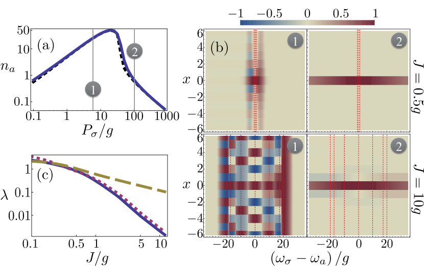
Figure 2: (a) Cavity population $n_{a}$ for $\omega_{\sigma}=\omega_{a}$ as a function of pump $P_{\sigma}$ for $J=0.5g$ (solid blue) and $J=10g$ (dashed black), with $N=12$, $\gamma_{a}=0.1g$, $\gamma_{\sigma}=0.01g$. (b) Corresponding first order correlations $\mathcal{C}(x)$ as a function of distance $x$ and emitter frequency $\omega_{\sigma}$ at pump rates (1) and (2) in plot (a). Bloch mode resonances are plotted as vertical dashed red lines. (c) Inverse correlation lengths, $\lambda$, as obtained from fits (see main text) for $N=108$, $P_{\sigma}=5g$, and $\Delta=0$ (solid), $\Delta=J$ (dotted) or $\Delta=2J$ (dashed).

Correlations in one dimension (1D).—We now examine correlations in a 1D chain, $\mathcal{C}(x)$ with $-N/2\leq x\leq N/2$, Eq. (4), considering $N$ to be a multiple of 4, so that the Bloch modes are distributed symmetrically around the cavity frequency. We first focus on $N=12$ with $J=0.5g$ or $10g$, for which we show $n_{a}$ as a function of the pump in Fig. 2(a). Both cases undergo very similar and characteristic transitions into and out of lasing (c.f. Fig. 1($i$)). We select two pumping rates representative of the lasing (1) and thermal (2) regimes and plot $\mathcal{C}(x)$ as a function of detuning $\Delta=\omega_{\sigma}-\omega_{a}$ and the separation $x$ between the cavities in Fig. 2(b). For $|\Delta|<2J$, $\mathcal{C}(x)$ oscillates as $\cos(\overline{k}x)$, where $\overline{k}$ and $-\overline{k}$ are the (degenerate) modes closest to resonance with the emitters, i.e. $|\Delta|\approx 2J\cos\overline{k}$. The correlation length is longer in the lasing regime (1), increases for larger $J$ and becomes maximal for $|\Delta|=2J$ in each case, i.e. when the emitters are in resonance with the edges of the Bloch band. For $J=10g$ it becomes larger than the finite size array of $N=12$ considered here since the frequency separation between Bloch modes is so large that the emitters only populate one mode efficiently. Note that any decay of correlations is entirely due to destructive interference between different Bloch-mode contributions.

Let us now explore $|\Delta|\leq 2J$, where the emitters are on resonance with the Bloch band and photonic modes are appreciably populated. For a long chain, $N\gg 1$, and large tunneling rates, $J\gg g$, analytical estimates can be found for the correlations $\mathcal{C}(x)$ sup . In agreement with Fig. 2, these show exponential decay modulated by an oscillation. We thus fit a function $f(x)=[c_{1}\cos(\nu x)+c_{2}\sin(\nu x)]\exp(-\lambda x)$ to $\mathcal{C}(x)$ in the entire range of tunneling rates $J$ and extract the inverse correlation length, $\lambda$, from the fit (see sup for examples). Fig. 2(c) shows $\lambda$ for three cases: $\Delta=0$ (solid), $\Delta=J$ (dotted) and $\Delta=2J$ (dashed) for a chain of $N=108$ cavities, which has Bloch modes in resonance with the emitters for all considered values of $\Delta$ so that finite-size effects are suppressed. As second main result of our work we observe a clear transition from the regime with $J<g$, where $\lambda\propto-\ln J$, to the regime $J>g$, where $\lambda\propto J^{-1}$ for $J\gg|\Delta|$ and $\lambda\propto J^{-1/2}$ for $2J=|\Delta|$ sup . These behaviors are also found from analytical estimates for $N\to\infty$ sup .

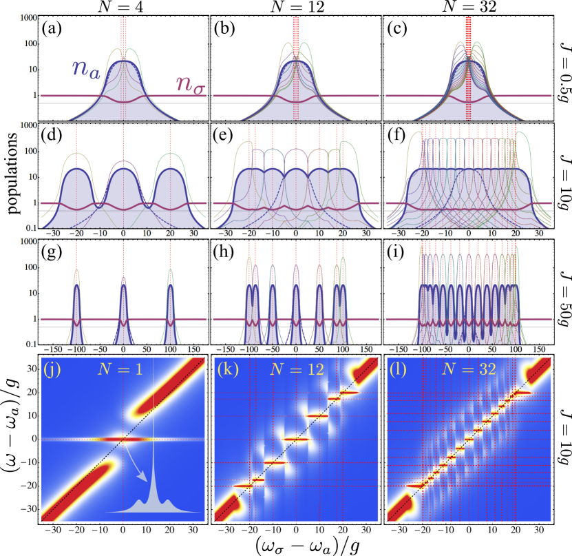
Figure 3: (a)–(i) Populations of the different modes involved, when sweeping the emitter frequency $\omega_{\sigma}$ through the system resonances (vertical red dashed lines): $n_{a}$ in solid and filled blue, $n_{\sigma}$ in solid pink, the Bloch modes $n_{k}$ with thin lines and $n_{a}$ for the case $N=1$ in dashed blue as a reference. (j) Emitter spectrum of emission for $N=1$ and varying $\omega_{\sigma}$, showing a Mollow triplet around resonance. In inset, the lineshape at resonance. In (k) and (l), the spectra for cases (e) and (f), respectively. We use a temperature color code which goes from blue (0) to red (maximum values). Parameters are $N=4$, 12, 32 and $J=0.5g$, $10g$, $50g$, varying as indicated. Also: $P_{\sigma}=5g$, $\gamma_{a}=0.1g$, $\gamma_{\sigma}=0.01g$.

Local properties in 1D chains.—Finally, we present some experimentally observable and distinctive local signatures of the collective lasing regime in the array, as a function of $\Delta$. In Fig. 3(a)–(i) we plot $n_{a}$ and $n_{\sigma}$, computed from Eqs. (2), for various arrays. Each underlying Bloch mode $n_{k}$ enters its own lasing regime at $\omega_{\sigma}=\omega_{k}$. This results in the enhancement of $n_{a}$ to a fixed value, given by the resonant one-emitter case $n_{a}^{\mathrm{L}}$, while the emitter population decreases to $n_{\sigma}^{\mathrm{L}}\approx 1/2$ from its saturation value of 1. Note that these traits are independent of $g$, $N$ and $J$ once the system is strongly enough coupled to reach the lasing regime Laussy et al. (2012). Interactions as small as $J\lesssim 0.5g$ (Fig. 3 upper row) are not enough to make a qualitative difference from the $N=1$ case in the local populations. The width in detuning of the apparent single broad resonance is given by $2\Delta_{\mathrm{max}}=\sqrt{P_{\sigma}(\kappa_{\sigma}-P_{\sigma})}$ . Increasing interactions, $J>g$ (other rows), splits the Bloch modes apart so that they can be selectively addressed by changing detuning. The excitation is distributed equally among the driven modes so, at resonance, $n_{k=0,\pi}=Nn_{a}^{\mathrm{L}}$ and $n_{\pm k}=Nn_{a}^{\mathrm{L}}/2$ for the other central modes. This results in a series of peaks for $n_{a}$ of equal height $n_{a}^{\mathrm{L}}$ and width $2\Delta_{\mathrm{max}}$. When the width is smaller than the average separation between Bloch modes, approximately given by $4J/N$ (or $4J/(N-1)$ for odd $N$), a plateau forms in the populations that extends for $|\Delta|\leq 2J$, c.f. Fig. 3(f). At this point, increasing $N$ does not affect the results qualitatively.

Another very distinctive feature of the collective lasing is provided by the PL spectrum. Despite the incoherent pump, a Mollow triplet forms Mollow (1969); del Valle and Laussy (2010, 2011, 2013) whenever $\omega_{\sigma}=\omega_{k}$ for some $k$, thanks to the effective multi-Bloch-mode coherent drive $\Omega(t)=\sum_{k}g\sqrt{n_{k}/N}e^{-i\omega_{k}t}$ sup . In Fig. 3(j)–(l), we compare $N=1$, 12 and 32, for varying $\Delta$. The Rayleigh peak, pinned at the laser frequency for a single mode excitation Mollow (1969), jumps from Bloch mode to Bloch mode, depending on which one dominates, in correspondence with the population plateaus of Fig. 3(e), (f). The sidebands are positioned at $\omega_{k}\pm 2\sqrt{2}g\sqrt{n_{a}^{\mathrm{L}}}$, around resonance with a degenerate Bloch mode $\omega_{k}$, and at $\omega_{k}\pm 2g\sqrt{n_{a}^{\mathrm{L}}}$, with the edge modes. Therefore, high $N$ and closely packed Bloch modes give rise to two Mollow continuous sidebands at $\omega_{\sigma}\pm 2\sqrt{2}g\sqrt{n_{a}^{\mathrm{L}}}$, extending over $|\Delta|\leq 2J$.

Acknowledgements.—JR-R acknowledges the hospitality of Technical University Munich, where part of this work was done. EdV acknowledges support from the Alexander von Humboldt-Foundation and the Spanish MINECO under contract MAT2011-22997 and MJH from the Emmy Noether grant HA 5593/1-1 and the CRC 631 (both DFG).

Supplemental Material

Appendix A I. Equations of motion for the correlators

In this section, we derive the system equations of motion in the case of a one-dimensional array. They can be trivially extended to higher dimensions.

The most general operator in the system reads $\langle O\rangle=\langle\Pi_{k}p_{k}^{\dagger m_{k}}p_{k}^{n_{k}}\Pi_{j}\sigma_{1}^{\dagger\mu_{j}}\sigma_{1}^{\nu_{j}}\rangle$. From the master equation in the main text, we obtain the equations of motion for the set of relevant operators by means of the general relation $\partial_{t}\langle O\rangle=\mathrm{Tr}(O\partial_{t}\rho)$ as

$$\partial_{t}\langle\Pi_{k}p_{k}^{\dagger m_{k}}p_{k}^{n_{k}}\Pi_{j}\sigma_{1}^{\dagger\mu_{j}}\sigma_{1}^{\nu_{j}}\rangle=\sum_{\bar{m}_{1},\bar{n}_{1},\ldots\bar{\mu}_{1},\bar{\nu}_{1}\dots}\\ R_{\tiny\begin{array}[]{c}m_{1},n_{1},\ldots\mu_{1},\nu_{1}\dots\\ \bar{m}_{1},\bar{n}_{1},\ldots\bar{\mu}_{1},\bar{\nu}_{1}\dots\end{array}}\langle\Pi_{k}p_{k}^{\dagger\bar{m}_{k}}p_{k}^{\bar{n}_{k}}\Pi_{j}\sigma_{1}^{\dagger\bar{\mu}_{j}}\sigma_{1}^{\bar{\nu}_{j}}\rangle\,.$$ (1)

The diagonal elements in $R$, involving all modes and emitters, are given by del Valle (2010):

$$R_{\tiny\begin{array}[]{c}m_{1},n_{1},\ldots\mu_{1},\nu_{1}\dots\\ m_{1},n_{1},\ldots\mu_{1},\nu_{1}\dots\end{array}}=$$

$$\sum_{k}[i\omega_{k}(m_{k}-n_{k})-\frac{\gamma_{a}}{2}(m_{k}+n_{k})]$$

$$+ \sum_{j}[i\omega_{\sigma}(\mu_{j}-\nu_{j})-\frac{\gamma_{\sigma}+P_{\sigma}}{2}(\mu_{j}+\nu_{j})-\frac{\gamma_{\phi}}{2}(\mu_{j}-\nu_{j})^{2}]\,.$$

We have included in these elements the effect of pure dephasing at a rate $\gamma_{\phi}$, added to the master equations through the Lindblad term $\gamma_{\phi}\mathcal{L}_{\sigma_{j}^{\dagger}\sigma_{j}}(\rho)$. This only results in the increase of the total decoherence rate into $\Gamma=\gamma_{a}+P_{\sigma}+\gamma_{\sigma}+\gamma_{\phi}$ Gonzalez-Tudela et al. (2010). Next, the incoherent pumping of emitter $j$ affects only elements concerning such emitter so that for all $j$:

$$R_{\tiny\begin{array}[]{c}\ldots\mu_{j},\nu_{j}\dots\\ \ldots\mu_{j},\nu_{j}\dots\end{array}}=P_{\sigma}\mu_{j}\nu_{j}\,.$$ (5)

Finally, the coupling between mode $k$ and emitter $j$, provides the elements:

$$R_{\tiny\begin{array}[]{c}m_{k},n_{k},\mu_{j},\nu_{j}\\ m_{k}-1,n_{k},1-\mu_{j},\nu_{j}\end{array}}=iG_{kj}m_{k}(1-\mu_{j})\,,$$ (6c)

$$R_{\tiny\begin{array}[]{c}m_{k},n_{k},\mu_{j},\nu_{j}\\ m_{k},n_{k}-1,\mu_{j},1-\nu_{j}\end{array}}=-iG_{kj}^{*}n_{k}(1-\nu_{j})\,,$$ (6f)

$$R_{\tiny\begin{array}[]{c}m_{k},n_{k},\mu_{j},\nu_{j}\\ m_{k}+1,n_{k},1-\mu_{j},\nu_{j}\end{array}}=iG_{kj}^{*}\mu_{j}\,,$$ (6i)

$$R_{\tiny\begin{array}[]{c}m_{k},n_{k},\mu_{j},\nu_{j}\\ m_{k},n_{k}+1,\mu_{j},1-\nu_{j}\end{array}}=-iG_{kj}\nu_{j}\,$$ (6l)

$$R_{\tiny\begin{array}[]{c}m_{k},n_{k},\mu_{j},\nu_{j}\\ m_{k}+1,n_{k},\mu_{j},1-\nu_{j}\end{array}}=-2iG_{kj}^{*}\mu_{j}(1-\nu_{j})\,,$$ (6o)

$$R_{\tiny\begin{array}[]{c}m_{k},n_{k},\mu_{j},\nu_{j}\\ m_{k},n_{k}+1,1-\mu_{j},\nu_{j}\end{array}}=2iG_{kj}\nu_{j}(1-\mu_{j})\,,$$ (6r)

and zero everywhere else.

With these general rules, we can write the equations for the main correlators of interest, starting with the populations of the modes, $n_{k}=\langle p^{\dagger}_{k}p_{k}\rangle$ and emitters $n_{j}=\langle\sigma_{j}^{\dagger}\sigma_{j}\rangle$:

$$\partial_{t}n_{j}=-(P_{\sigma}+\gamma_{\sigma})n_{j}+P_{\sigma}-2\sum_{k}\Im[G_{kj}^{*}\langle p_{k}^{\dagger}\sigma_{j}\rangle]\,,$$ (7a)

$$\partial_{t}n_{k}=-\gamma_{a}n_{k}+2\sum_{j}\Im[G_{kj}^{*}\langle p_{k}^{\dagger}\sigma_{j}\rangle]\,,$$ (7b)

$$\partial_{t}\langle p_{k}^{\dagger}\sigma_{j}\rangle=-[\frac{\Gamma}{2}+i(\omega_{\sigma}-\omega_{k})]\langle p_{k}^{\dagger}\sigma_{j}\rangle$$

$$+iG_{kj}[n_{j}-n_{k}+2\langle p_{k}^{\dagger}p_{k}\sigma_{j}^{\dagger}\sigma_{j}\rangle]$$

$$+\sum_{l\neq j}iG_{kl}\langle\sigma_{l}^{\dagger}\sigma_{j}\rangle+\sum_{q\neq k}(-iG_{ql})\langle p_{k}^{\dagger}p_{q}\rangle$$

$$+\sum_{q\neq k}2iG_{qj}\langle p_{k}^{\dagger}p_{q}\sigma_{j}^{\dagger}\sigma_{j}\rangle\,.$$ (7c)

The equations for the correlators that represent the indirect coupling between different emitters or Bloch modes are:

$$\partial_{t}\langle\sigma_{l}^{\dagger}\sigma_{j}\rangle=-(P_{\sigma}+\gamma_{\sigma})\langle\sigma_{l}^{\dagger}\sigma_{j}\rangle$$

$$+\sum_{k}i[G_{kl}^{*}\langle p_{k}^{\dagger}\sigma_{j}\rangle-G_{kj}\langle p_{k}\sigma_{l}^{\dagger}\rangle]$$

$$+\sum_{k}2i[G_{kj}\langle p_{k}\sigma_{l}^{\dagger}\sigma_{j}^{\dagger}\sigma_{j}\rangle-G_{kl}^{*}\langle p_{k}^{\dagger}\sigma_{l}^{\dagger}\sigma_{l}\sigma_{j}\rangle]\,,$$ (8a)

$$\partial_{t}\langle p_{k}^{\dagger}p_{q}\rangle=-[\gamma_{a}-i(\omega_{k}-\omega_{q})]\langle p_{k}^{\dagger}p_{q}\rangle$$

$$+\sum_{j}i[G_{kj}\langle p_{q}\sigma_{j}^{\dagger}\rangle-G^{*}_{qj}\langle p_{k}^{\dagger}\sigma_{j}\rangle]\,.$$ (8b)

Within the formal scheme of the Cluster-Expansion method, Eq. (8a) is of the same order as the Bloch-mode populations $n_{k}$. This is owed to the dominant Jaynes-Cummings interaction in the system, which can be used to establish a formal equivalence between an electronic transition and photon creation or absorption Gies et al. (2007). In the thermal and lasing regimes investigated in the main text, the influence of these correlations is small and, therefore, neglected in order to keep the formal solution of the equations as simple as possible.

Finally, the intensity-intensity correlations are given by:

$$\partial_{t}\langle p_{k}^{\dagger}p_{k}\sigma_{l}^{\dagger}\sigma_{l}\rangle=-(\gamma_{a}+P_{\sigma}+\gamma_{\sigma})\langle p_{k}^{\dagger}p_{k}\sigma_{l}^{\dagger}\sigma_{l}\rangle+P_{\sigma}n_{k}$$

$$+i(G_{kl}^{*}\langle p_{k}^{\dagger}p_{k}^{\dagger}p_{k}\sigma_{l}\rangle-G_{kl}\langle p_{k}^{\dagger}p_{k}p_{k}\sigma_{l}^{\dagger}\rangle)$$

$$+i\sum_{q\neq k}(G_{ql}^{*}\langle p_{q}^{\dagger}p_{k}^{\dagger}p_{k}\sigma_{l}\rangle-G_{ql}\langle p_{q}^{\dagger}p_{k}p_{k}\sigma_{l}^{\dagger}\rangle)$$

$$+i\sum_{j\neq l}(G_{kj}\langle p_{k}\sigma_{l}^{\dagger}\sigma_{l}\sigma_{j}^{\dagger}\rangle-G_{kj}^{*}\langle p_{k}^{\dagger}\sigma_{j}\sigma_{l}^{\dagger}\sigma_{l}\rangle)\,.$$ (9)

Thanks to the translational invariance in the array (which leads to linear momentum conservation), the Bloch mode correlations vanish, $\langle p_{\vec{k}}^{\dagger}p_{\vec{q}}\rangle=\delta_{\vec{k},\vec{q}}n_{\vec{k}}$, and the cavity correlations are simply the Fourier transform of the Bloch mode populations:

$$\langle a_{j}^{\dagger}a_{j+x}\rangle=\frac{1}{N}\sum_{k}e^{-ixk}n_{k}\,,$$ (10)

and Eq. (4) from the main text, more generally stated in any dimension.

Analytical solutions of the rate equations for $N=1$

In the case $N=1$, we have only a single emitter and photonic mode so $F_{k}\rightarrow F$ and the rate equations in the steayd state reduce to:

$$0=-\gamma_{a}n_{a}+Fn_{a}(2n_{\sigma}-1)+Fn_{\sigma}\,,$$

$$0=-(P_{\sigma}+\gamma_{\sigma}+F)n_{\sigma}+P_{\sigma}-(2n_{\sigma}-1)Fn_{a}\,.$$

The solution of these equations reads,

$$n_{a} = \frac{F(2P_{\sigma}-\zeta_{\sigma}-\gamma_{a})-\gamma_{a}\zeta_{\sigma}+\chi^{2}}{4F\gamma_{a}}\,,$$ (12)

$$n_{\sigma} = \frac{P_{\sigma}-\gamma_{a}n_{a}}{\zeta_{\sigma}}$$ (13)

with $\chi^{2}=\sqrt{[F(2P_{\sigma}+\zeta_{\sigma}+\gamma_{a})+\gamma_{a}\zeta_{\sigma}]^{2}-8FP_{\sigma}\zeta_{\sigma}(F+\gamma_{a})}$ and $\zeta_{\sigma}=P_{\sigma}+\gamma_{\sigma}$.

Appendix B II. Fast decay of correlations

Here we consider a rectangular $m$-dimensional lattice of cavities in the thermodynamic limit, i.e. where infinitely many cavities are arranged in each lattice direction. We thus have a continuum of momentum modes and $\frac{1}{N^{m}}\sum_{\vec{k}}$ turns into an integral over the Brillouin Zone (BZ) $V_{k}$ formed by the $m$-dimensional cube extending from $-\pi$ to $\pi$ in each direction.

The field correlations are given by

$$\mathcal{C}(\vec{r})=\frac{\langle a_{\vec{0}}^{\dagger}a_{\vec{0}+\vec{r}}\rangle}{\langle a_{\vec{0}}^{\dagger}a_{\vec{0}}\rangle}=\frac{1}{n_{a}\,(2\pi)^{m}}\int_{V_{k}}d^{m}ke^{-i\vec{k}\vec{r}}n(\vec{k}),$$ (14)

with $\vec{r}$ running on the lattice of $m$-dimensional vectors with integer coordinates.

For $\delta^{2}>0$, $n(\vec{k})$ is a continuous function of $k$ defined on a finite domain, and therefore it is integrable over $V_{k}$. In this case the Riemann-Lebesgue lemma  Rudin (1987) ensures that $\mathcal{C}(\vec{r})$ decays to zero for $\vec{r}\to\infty$. The result we want to show is that this decay is actually faster than any power of $r$. The proof relies essentially on the fact that $n(\vec{k})$ depends on $\vec{k}$ through cosine functions of the components of $\vec{k}$. As such, $n(\vec{k})$ and all its derivatives are continuous and periodic functions of $\vec{k}$. By periodicity here we mean invariant with respect to translations by reciprocal lattice vectors, i.e. $n(\vec{k})=n(\vec{k}+\vec{K})$, where the coordinates of $\vec{K}$ are integer multiples of $2\pi$. In particular, on the surface of the BZ one finds pairwise opposite points, differing by a reciprocal lattice vector. It follows that in such points $n(\vec{k})$ has equal values, and the same is true for all its derivatives.

For the proof we denote by $\alpha=\{\alpha_{1},\alpha_{2}\dots\alpha_{m}\}$ a multi-index of natural numbers and by $|\alpha|$ the sum of its components $\alpha_{1}+\dots\alpha_{m}$. We denote also by $r^{\alpha}$ the quantity $r_{1}^{\alpha_{1}}r_{2}^{\alpha_{2}}\dots r_{m}^{\alpha_{m}}$. The result we want to show is that for any $\alpha$ one has $r^{\alpha}\mathcal{C}(\vec{r})\to 0$ when $r\to\infty$.

Indeed, multiplying the integral in Eq. (14) with $r^{\alpha}$ amounts to applying the derivative operator $(i\partial)^{\alpha}=i^{|\alpha|}\partial_{1}^{\alpha_{1}}\dots\partial_{m}^{\alpha_{m}}$ to the plane-wave factor $e^{-i\vec{k}\vec{r}}$ under the integral. By $\partial_{i}$ we mean the derivative with respect to $k_{i}$. All these derivatives can be transferred upon $n(\vec{k})$ by repeatedly applying the divergence theorem. At each such step, BZ surface integrals are generated. But each of these integrals vanishes, because it involves pairwise equal values of the integrand at the opposite points of the BZ surface. The outer normals to the surface in such points have opposite orientation and this ensures the cancellation. Note that in this argument both the periodicity of the derivatives of $n(\vec{k})$ and that of $e^{-i\vec{k}\vec{r}}$ are required. The latter is ensured by $\vec{r}$ having integer coordinates.

After trasferring all the derivatives one is left with

$$r^{\alpha}\mathcal{C}(\vec{r})=\frac{(-i)^{|\alpha|}}{n_{a}\,(2\pi)^{m}}\int_{V_{k}}d^{m}ke^{-i\vec{k}\vec{r}}\partial^{\alpha}n(\vec{k})\,.$$ (15)

Since the integrand is again a continuous function, the Riemann-Lebesgue lemma can be invoked again, ensuring that, indeed, $r^{\alpha}\mathcal{C}(\vec{r})$ goes to zero for large values of the argument. This concludes the proof.

The only possibility that the correlation length could diverge is thus a case where $(2n_{\sigma}-1)=\Gamma/\kappa_{\sigma}$, for which $n_{\vec{k}}\propto\Delta_{\vec{k}}^{-2}$. For this case, however, the last term in Eq. (2b) in the main text, which reads $(2n_{\sigma}-1)\frac{1}{n_{a}\,(2\pi)^{m}}\int_{V_{k}}d^{m}kF_{\vec{k}}n_{\vec{k}}$, diverges as long as $(2n_{\sigma}-1)\neq 0$. The origin of this divergence is that $\Delta_{\vec{k}}^{-2}$ at least scales as $\Delta_{\vec{k}}^{-2}\propto(k_{\alpha}-\overline{k}_{\alpha})^{-2}$ in the vicinity of a manifold $\overline{k}$ where $\Delta_{\vec{k}}=0$ (if $\Delta_{\vec{k}}=0$ occurs at the boundary of the integration volume the divergence is even more severe). We thus conclude that non-exponential decay or a divergent correlation length can only appear for $\delta=0$ and $(2n_{\sigma}-1)=0$. Both conditions can only hold for $\gamma_{a}=0$, i.e. if the photon decay vanishes.

Estimates for field correlations in one dimension in the limit $N\to\infty$

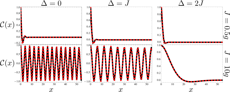
Figure 1: Examples for fits of functions $f(x)=[c_{1}\cos(\nu x)+c_{2}\sin(\nu x)]\exp(-\lambda x)$ to the normalized correlations $\mathcal{C}(x)$ for $N=108$ and the parameters $\Delta$ and $J$ given in the labels of the columns and rows. Other parameters are $\gamma_{a}=0.1g$, $\gamma_{\sigma}=0.01g$, $P_{\sigma}=5g$.

For one dimension, $m=1$, the momentum distribution in the stationary state reads, $n_{k}=\frac{\kappa_{\sigma}\Gamma}{4}\frac{n_{\sigma}}{(\delta/2)^{2}+\Delta_{k}^{2}}$, which is a Lorentzian in the detunings $\Delta_{k}=\Delta-2J\cos k$, and for $N\to\infty$ the field correlations read,

$$\mathcal{C}(x)=\frac{1}{n_{a}2\pi}\int_{-\pi}^{\pi}dke^{-ixk}n_{k}\,.$$ (16)

With $n_{k}$ a real and even function of $k$, it is obvious that $\mathcal{C}(x)$ is also real and even as a function of the distance $x$. Therefore in what follows we consider only the case $x\geqslant 0$. Up to the prefactor $\frac{\kappa_{\sigma}\Gamma n_{\sigma}}{4n_{a}J^{2}}$, and bearing in mind that $x$ takes only integer values, the correlations are obtained by calculating a Fourier transform of the form

$$C_{n}=\frac{1}{2\pi}\int_{-\pi}^{\pi}\,\frac{e^{ikn}}{(2\cos k-\widetilde{\Delta})^{2}+\widetilde{\delta}^{2}}\,dk,\quad n=0,1\dots$$ (17)

with the parameters $\widetilde{\Delta}$ and $\widetilde{\delta}$ easy to identify as $\widetilde{\Delta}=\Delta/J$ and $\widetilde{\delta}=\delta/(2J)$. One rearranges the expression under the intergal as

$$\frac{1}{(2\cos k-\widetilde{\Delta})^{2}+\widetilde{\delta}^{2}}=\frac{1}{2i\widetilde{\delta}}\,\frac{1}{2\cos k-\widetilde{\Delta}-i\widetilde{\delta}}+\text{c.c.}\,,$$ (18)

so that one has to compute

$$C_{n}=\frac{1}{4\pi i\widetilde{\delta}}\int_{-\pi}^{\pi}\,\frac{e^{ikn}}{2\cos k-u}\,dk+\text{c.c.}\,,$$ (19)

where $u$ denotes the complex quantity $u=\widetilde{\Delta}+i\widetilde{\delta}=J^{-1}(\Delta+i\delta/2)$. This integral is solved by introducing the new variable $z=e^{ik}$, which runs on the unit circle ${\cal C}_{1}$,

$$C_{n}=\frac{-1}{4\pi\delta}\int_{{\cal C}_{1}}\frac{z^{n}}{z^{2}-u\,z+1}\,dz+\text{c.c.}\,.$$ (20)

The poles of the integrand are the roots of the denominator $\zeta_{1,2}$, and satisfy $\zeta_{1}+\zeta_{2}=u$ and $\zeta_{1}\,\zeta_{2}=1$. There are two possibilities, either (i) $|\zeta_{1}|<1<|\zeta_{2}|$, or (ii) $|\zeta_{1}|=1=|\zeta_{2}|$. Representing the roots as $\zeta_{2}=e^{\lambda}e^{iq}$ and $\zeta_{1}=e^{-\lambda}e^{-iq}$, case (i) amounts to $\lambda>0$ and $\zeta_{1}$ lying inside the unit circle. The residue theorem then gives

$$C_{n}=\frac{i}{2\widetilde{\delta}}\,\frac{1}{\zeta_{2}-\zeta_{1}}\,\zeta_{1}^{n}+\text{c.c.}\,.$$ (21)

This shows that the correlations oscillate along the chain with a wave number $q$ and decay exponentially with the inverse decay length $\lambda$.

Case (ii) corresponds to $\lambda=0$, when both roots are found on ${\cal C}_{1}$. This takes place when $u=\zeta_{1}+\zeta_{2}=2\cos q$ i.e. $u$ is real and belongs to the interval $[-2,2]$. With poles on the integration path the integral is divergent. Still, it makes sense to consider this as a limit case, with $u$ approaching the segment $[-2,2]$ of the real axis. Then $\zeta_{1}$ approaches the unit circle from within, and the correlation length $1/\lambda$ goes to infinity. The system becomes critical. The requirements on the system parameters for achieving criticality are $\delta\to 0$ and $|\Delta|\leqslant 2J$. It also follows that $q$ is the momentum of the resonant Bloch mode.

It is straightforward to relate the quantities $\lambda$ and $q$, to the system parameters but the expressions are cumbersome. Some qualitative features are easily obtained though, and they describe different regimes of correlation behaviour.

A first situation is encountered when $u$ lies in the complex plane far away from the critical interval $[-2,2]$. For $\widetilde{\Delta}$ and $\widetilde{\delta}$ large, this corresponds to small $J$-values, since $\widetilde{\Delta}\propto J^{-1}$ and $\widetilde{\delta}\propto J^{-1}$ In this case $\lambda$ is large and in the relation $\zeta_{1}+\zeta_{2}=u$ the small root $\zeta_{1}$ becomes negligible. It follows that $\lambda=\ln|\zeta_{2}|\simeq\ln|u|\propto-\ln J$.

A completely different behavior is seen when $u$ is close to the segment $[-2,2]$. In this regime $J$ is large to make $\widetilde{\delta}$ small. Also, $\Delta$, $J$ are of the same magnitude and obey $|\Delta|\leqslant 2J$, to keep $\widetilde{\Delta}$ within the limit of the interval. In this case $\lambda\simeq 0$, both roots are close to the unit circle. Therefore both contribute to the sum, and one can write

$$\frac{1}{2}u=\frac{1}{2}(\widetilde{\Delta}+i\widetilde{\delta})=\cosh\lambda\cos q+i\sinh\lambda\sin q\,.$$ (22)

With $\lambda$ small, one has $\cosh\lambda\simeq 1$ and $\sinh\lambda\simeq\lambda$ and by identifying the real and imaginary parts, it follows that $\cos q=\widetilde{\Delta}/2=\Delta/(2J)$ and

$$\lambda =\frac{\widetilde{\delta}}{2\sin q}=\frac{\delta/2}{\sqrt{4J^{2}-\Delta^{2}}}$$

$$=\sqrt{\frac{g^{2}\Gamma}{\gamma_{a}(4J^{2}-\Delta^{2})}\left[\frac{\gamma_{a}\Gamma}{4g^{2}}-(2n_{\sigma}-1)\right]}\,.$$ (23)

With $\Delta$ of the same order as $J$, one obtains $\lambda\propto J^{-1}$.

The above result holds for $\widetilde{\Delta}$ not too close to the endpoints of the critical interval, where $\sin q$ becomes small and division by it gives rise to large values of $\lambda$. This is seen in the final expression for $\lambda$, in which $\Delta$ approaching $2J$ leads to a singularity. Therefore this case requires a separate, more careful consideration, since now $q$ becomes a small quantity, too. Expanding up to the second order in terms of the small arguments, Eq. (22) becomes

$$\frac{1}{2}(\widetilde{\Delta}+i\widetilde{\delta})\simeq 1+\frac{1}{2}\lambda^{2}-\frac{1}{2}q^{2}+i\lambda\,q\,.$$ (24)

To keep the discussion simple we discuss the case $\Delta=2J$, or $\widetilde{\Delta}=2$. Actually this illustrates the more general situation in which $1-\widetilde{\Delta}/2$ is a small quantity of a higher than second order. Then, from Eq. (24) we find $\lambda=q$ and $\lambda^{2}=\widetilde{\delta}/2=\delta/(4J)$. More precisely

$$\lambda=\left\{\frac{g^{2}\Gamma}{4\gamma_{a}J^{2}}\left[\frac{\gamma_{a}\Gamma}{4g^{2}}-(2n_{\sigma}-1)\right]\right\}^{1/4}\,.$$ (25)

Note that now $\lambda\propto J^{-1/2}$.

Examples for the fits

In this section we provide some examples for the fits of functions $f(x)=[c_{1}\cos(\nu x)+c_{2}\sin(\nu x)]\exp(-\lambda x)$ to the normalized correlations $\mathcal{C}(x)$. These examples are shown in Fig. 1 and illustrate the excellent quality of the fits. Only for $J\ll g$ the fitting procedure is more fragile as correlations decay very fast and are thus indistinguishable from zero for most values of $x$.

Appendix C III. Derivation of the emitter spectrum of emission

In this section we obtain the emitter photoluminescence spectrum $S(\Gamma_{d},\omega)$, in the lasing regime, where $\Gamma_{d}$ is the detector linewidth. We make the semiclassical approximation of substituting the cavity fields by a multimode laser that acts independently on each of the emitters. That is, we consider the approximated Hamiltonian $H_{\mathrm{ML}}=\sum_{\vec{r}}[\omega_{\sigma}{\sigma_{\vec{r}}^{\dagger}}\sigma_{\vec{r}}+\Omega(t){\sigma_{\vec{r}}^{\dagger}}+\Omega^{*}(t)\sigma_{\vec{r}}]$, where $\Omega(t)=\sum_{\vec{k}}g\sqrt{n_{\vec{k}}/N}e^{-i\omega_{\vec{k}}t}$ is the time-dependent multimode field. Additionally, the emitters are still being excited by the incoherent pump and decay that act on their dynamics through the usual Lindblad forms. There is no steady state for this approximated model (for $N>1$) but a quasi-steady state, that is, an ever oscillating solution for the density matrix elements around a mean point. Such mean point is given (approximately) by the exact solution of the full master equation or the rate equations, which do have a steady state. That is, $\sum_{\vec{k}}G_{\vec{k}\vec{r}}\langle p_{\vec{k}}\sigma_{\vec{r}}^{\dagger}\rangle e^{-i\omega_{\vec{k}}t}$ is well estimated by $\Omega(t)\langle\sigma_{\vec{r}}^{\dagger}\rangle_{\mathrm{ML}}$, where $\langle\cdot\rangle_{ML}$ is the mean value obtained with the approximated master equation and Hamiltonian $H_{ML}$ for the emitters only. The fact that the first term is $\vec{r}$-independent, compels $\Omega(t)$ to be $\vec{r}$-independent as well. We describe the resulting time-dependent dynamics in the following way: First, we solve the new master equation with $H_{\mathrm{ML}}$, and obtain its time-dependent spectrum of emission Eberly and Wódkiewicz (1977); Eberly et al. (1980), $S_{\mathrm{ML}}(\Gamma_{d},\omega,t)$, by coupling the emitter very weakly to another two-level system, which radiatively decays at a rate $\Gamma_{d}$, and plays the role of the detector. The population of this detector is exactly the time-dependent spectrum of our emitter del Valle et al. (2012). Then, we take its average over time, once the quasi-steady state is reached, starting at a point in time which we call $t_{0}$: $S(\Gamma_{d},\omega)\approx\int_{t_{0}}^{t_{0}+T}S_{\mathrm{ML}}(\Gamma_{d},\omega,t)dt/T$. This is a very good approximation in the case $N=1$ del Valle and Laussy (2010, 2011) for which there is a simple analytical formula del Valle and Laussy (2013). The Rayleigh peak, produced by the elastically scattered cavity laser field, is pinned at the cavity frequency, $\omega=\omega_{a}$, and has a small linewidth given by the detector only $\Gamma_{d}$ (as in this approximation the cavity has an infinitely long lifetime). We used $\Gamma_{d}=0.3g$ to plot the spectra in Fig. 3(j)–(l) of the main text.

References

Hartmann et al. (2006)M. J. Hartmann, F. G. S. L. Brandão, and M. B. Plenio, Nat.
Phys. 2, 849 (2006).
Greentree et al. (2006)A. D. Greentree, C. Tahan,
J. H. Cole, and L. C. L. Hollenberg, Nat. Phys. 2, 856 (2006).
Diehl et al. (2008)S. Diehl, A. Micheli,
A. Kantian, B. Kraus, H. P. Bucheler, and P. Zoller, Nat. Phys. 4, 878 (2008).
Schindler et al. (2013)P. Schindler, M. Müller,
D. Nigg, J. T. Barreiro, E. A. Martinez, M. Hennrich, T. Monz, S. Diehl, P. Zoller, and R. Blatt, Nat. Phys. 9, 361 (2013).
Marcos et al. (2012)D. Marcos, A. Tomadin,
S. Diehl, and P. Rabl, New J. Phys. 14, 055005 (2012).
Altman et al. (2013)E. Altman, L. M. Sieberer, L. Chen,
S. Diehl, and J. Toner, (2013), arxiv:1311.0876 .
del Valle and Laussy (2010)E. del
Valle and F. P. Laussy, Phys.
Rev. Lett. 105, 233601
(2010).
Majumdar et al. (2012)A. Majumdar, A. Rundquist,
M. Bajcsy, V. D. Dasika, S. R. Bank, and J. Vuckovic, Phys. Rev. B 86, 195312
(2012).
Rundquist et al. (2013)A. Rundquist, A. Majumdar,
M. Bajcsy, V. D. Dasika, S. Bank, and J. Vuckovic, in CLEO: 2013 (Optical Society of America, 2013) p. CM4F.7.
Abbarchi et al. (2013)M. Abbarchi, A. Amo,
V. G. Sala, D. D. Solnyshkov, H. Flayac, L. Ferrier, I. Sagnes, E. Galopin, A. Lemaître, G. Malpuech, and J. Bloch, Nat. Phys. 9, 275 (2013).
Lepert et al. (2011)G. Lepert, M. Trupke,
M. J. Hartmann, M. B. Plenio, and E. A. Hinds, New J. Phys. 13, 113002 (2011).
del Valle et al. (2009)E. del
Valle, F. P. Laussy, and C. Tejedor, Phys. Rev. B 79, 235326 (2009).
Hartmann (2010b)M. J. Hartmann, Phys. Rev. Lett. 104, 113601 (2010b).
Averkiev et al. (2009)N. Averkiev, M. Glazov, and A. Poddubny, Sov. Phys. JETP 135, 959 (2009).
Note (1)This is only below the maximum cavity population, reached at
del Valle and Laussy (2011). We choose , and as a paradigmatic
example of the lasing regime for any .
Laussy et al. (2012) F. Laussy, E. del Valle, and J. Finley, Proc. SPIE 8255, 82551G (2012).
Note (2)Estimation obtained by solving in the detuned one-emitter laser del Valle and Laussy (2011).
Mollow (1969)B. R. Mollow, Phys.
Rev. 188, 1969 (1969).
del Valle and Laussy (2013)E. del
Valle and F. P. Laussy, Wolfram Demonstrations Project (2013).
del Valle (2010)E. del
Valle, Microcavity Quantum
Electrodynamics (VDM Verlag, 2010).
Gonzalez-Tudela et al. (2010)A. Gonzalez-Tudela, E. del
Valle, E. Cancellieri,
C. Tejedor, D. Sanvitto, and F. P. Laussy, Opt. Express 18, 7002 (2010).
Rudin (1987)W. Rudin, Real and Complex
Analysis (McGraw-Hill, 1987).
Eberly and Wódkiewicz (1977)J. Eberly and K. Wódkiewicz, J. Opt. Soc. Am. 67, 1252 (1977).
Eberly et al. (1980)J. H. Eberly, C. V. Kunasz,
and K. Wódkiewicz, J. phys. B.: At.
Mol. Phys. 13, 217
(1980).
del Valle et al. (2012)E. del
Valle, A. Gonzalez-Tudela, F. P. Laussy, C. Tejedor, and M. J. Hartmann, Phys. Rev. Lett. 109, 183601 (2012).