Population III Hypernovae

Abstract

Population III supernovae have been of growing interest of late for their potential to directly probe the properties of the first stars, particularly the most energetic events that are visible near the edge of the observable universe. But until now, hypernovae, the unusually energetic Type Ib/c supernovae that are sometimes associated with gamma-ray bursts, have been overlooked as cosmic beacons at the highest redshifts. In this, the latest of a series of studies on Population III supernovae, we present numerical simulations of 25 - 50 ${M}_{\odot}$ hypernovae and their light curves done with the Los Alamos RAGE and SPECTRUM codes. We find that they will be visible at $z=$ 10 - 15 to the James Webb Space Telescope (JWST) and $z=$ 4 - 5 to the Wide-Field Infrared Survey Telescope (WFIRST), tracing star formation rates in the first galaxies and at the end of cosmological reionization. If, however, the hypernova crashes into a dense shell ejected by its progenitor it is expected that a superluminous event will occur that may be seen at $z\sim$ 20, in the first generation of stars.

1. Introduction

Population III (Pop III) stars ended the cosmic Dark Ages and began cosmological reionization (e.g., Whalen et al., 2004; O’Shea et al., 2005; Whalen et al., 2008a, 2010) and the chemical enrichment of the IGM (Mackey et al., 2003; Smith & Sigurdsson, 2007; Smith et al., 2009; Ritter et al., 2012; Safranek-Shrader et al., 2014). They also populated the first galaxies (Johnson et al., 2009; Greif et al., 2010; Jeon et al., 2012; Pawlik et al., 2011; Wise et al., 2012; Pawlik et al., 2013) and may be the origin of supermassive black holes (e.g., Milosavljević et al., 2009; Alvarez et al., 2009; Tanaka & Haiman, 2009; Park & Ricotti, 2011; Johnson et al., 2012; Agarwal et al., 2012; Johnson et al., 2013c; Latif et al., 2013a, b; Johnson et al., 2014). Although they are very luminous, individual Pop III stars will not be visible to the James Webb Space Telescope ( JWST, Gardner et al., 2006), the Wide-Field Infrared Survey Telescope (WFIRST), or the Thirty-Meter Telescope (TMT; but see Rydberg et al., 2013, about detecting the H II regions of the first stars).

The fossil abundance record (the ashes of early supernovae thought to be imprinted on ancient metal-poor stars, e.g., Beers & Christlieb, 2005; Frebel et al., 2005) suggests that some Pop III stars were 15 - 50 ${M}_{\odot}$ (Joggerst et al., 2010). Numerical simulations of primordial star formation (O’Shea & Norman, 2007; Turk et al., 2009; Stacy et al., 2010; Clark et al., 2011; Smith et al., 2011; Greif et al., 2011a; Hosokawa et al., 2011; Greif et al., 2012; Stacy et al., 2012; Susa, 2013; Hirano et al., 2014) suggest that Pop III stars were 20 - 500 ${M}_{\odot}$ (for recent reviews, see Whalen, 2013; Glover, 2013). Together, these studies suggest that both high mass and low mass Pop III stars existed in the primeval universe, but they do not otherwise constrain their properties.

Primordial SNe (e.g, Whalen et al., 2008c) will be the first direct probes of the Pop III initial mass function (IMF) because they can be seen at great distances and the masses of their progenitors can be inferred from their light curves. Recent studies have shown that Pop III pair-instability (PI) SNe (Heger & Woosley, 2002; Fryer et al., 2010; Joggerst & Whalen, 2011; Kasen et al., 2011; Pan et al., 2012a, b; Hummel et al., 2012; Chatzopoulos & Wheeler, 2012; Chatzopoulos et al., 2013; Chen et al., 2014a) will be visible at $z\gtrsim$ 30 to deep-field surveys by JWST and at $z\sim 15-20$ in all-sky near infrared (NIR) surveys by WFIRST and the Wide-Field Imaging Surveyor for High Redshift (WISH) (Whalen et al., 2013a, c, d, 2014a; de Souza et al., 2013, 2014; Chen et al., 2014c; Smidt et al., 2014) (see also Johnson et al., 2013b; Whalen et al., 2013g, f; Chen et al., 2014b). PI SN candidates have now been identified at low redshifts (Gal-Yam et al., 2009; Cooke et al., 2012) (see also Whalen et al., 2014b). Others have found that JWST will detect Pop III core-collapse (CC) SNe at $z\sim$ 10 - 20, depending on the type of explosion (Whalen et al., 2013b, e, h) (see also Tominaga et al., 2011; Moriya et al., 2013; Tanaka et al., 2012, 2013).

In the past decade, hypernovae (HNe), with energies that are intermediate to those of CC and PI SNe, have been proposed to explain the elemental patterns found in hyper metal-poor stars (e.g., Maeda & Nomoto, 2003; Iwamoto et al., 2005; Tominaga et al., 2007) and to account for some unusually bright explosions (e.g., Nomoto et al., 2001; Mazzali et al., 2008). Although HNe are not fully understood, those observed to date have generally been Type Ib/c SNe and have been associated with gamma-ray bursts (GRBs, Iwamoto et al., 1998; Nakamura et al., 2001). They may therefore be explosions of massive stars that have shed their H envelopes and are bare He cores. Since Pop III stars are not generally thought to undergo pulsations (Baraffe et al., 2001) or have strong winds (Vink et al., 2001), the H layer is likely ejected during a common envelope phase with a binary companion. The central engine may be a black hole accretion disk system that drives a strong wind or jet that deposits part of its energy into the surrounding layers of the star. The result is a powerful, highly asymmetric explosion that can synthesize large amounts of ${}^{56}\mathrm{Ni}$, both of which may account for its brightness. Because their energies typically range from 10 - 50 $\times$ 10⁵¹ erg, HNe may be visible at redshifts intermediate to those at which PI and CC SNe can be detected. As such, they may be complementary probes of stellar populations in the primordial universe.

We have now calculated light curves and spectra for 25 - 50 ${M}_{\odot}$ Pop III HNe with the Los Alamos RAGE and SPECTRUM codes. In Section 2 we describe our grid of RAGE models and how we post process them with SPECTRUM to obtain light curves and spectra. In Section 3 we examine blast profiles, and in Section 4 we show NIR light curves and detection thresholds in redshift for HNe. In Section 5 we estimate Pop III HN event rates as a function of redshift, and we conclude in Section 6.

2. Numerical Models

We calculate light curves and spectra for HNe in three steps. First, stellar collapse and explosion is modeled in a 1D Lagrangian hydrodynamics code and its output is post processed with an astrophysical nuclear reaction network to obtain nucleosynthetic yields. After explosive burning is complete the blast profiles are ported to the RAGE code and evolved out to one year. We then post process our RAGE profiles with the SPECTRUM code to construct light curves and spectra.

2.1. Collapse and Explosion

To model collapse and explosion, we use the one-dimensional (1D) Lagrangian code and techniques described in Young & Fryer (2007). This code includes three-flavor neutrino transport with flux-limited diffusion and a coupled set of equations of state (EOS) to model the wide range of densities in the collapse phase (for details, see Herant et al., 1994; Fryer et al., 1999a). It includes a 14-element nuclear network (Benz et al., 1989) to follow energy generation. After collapse, bounce and formation of a proto-neutron star, we halt the run and remove the neutron star. To trigger the explosion we inject thermal energy into the innermost 15 zones (roughly 0.035 ${M}_{\odot}$). Convection mixes this energy fairly uniformly over the convective zone. We use 15 zones because they enclose the inner 0.1 ${M}_{\odot}$, which is roughly the mass of the convection zone. We have verified that varying the number of convection zones and enclosed mass (0.05 - 0.2 ${M}_{\odot}$) yields similar results.

The duration and magnitude of the energy injection in these artificial explosions were adjusted to vary the explosion energies. During energy injection, the proto neutron star is modeled as a hard surface. We do not include neutrino flux from the proto neutron star, but the energy injected by this flux is minimal compared to our artificial energy injection. Shortly after the end of the energy injection we change the hard neutron star surface to an absorbing boundary layer to capture the accretion of infalling matter due to neutrino cooling onto the proto neutron star. In this manner we can model the explosion out to late times, even if there is considerable fallback.

For more accurate yields, we post process our explosions with the public version of the torch code (Timmes, 1999) using the standard 489 isotope network. We explode a 25 ${M}_{\odot}$ Pop III star with energies of 10, 22, and 52 foe (1 foe $=$ 10⁵¹ erg) and a 50 ${M}_{\odot}$ star with energies of 10, 22, 52 and 92 foe. Profiles for these stars are taken from Woosley et al. (2002), and the masses and energies we have chosen bracket those inferred for HNe from observations. We resolve the inner regions of 25 and 50 ${M}_{\odot}$ stars with 3085 - 3092 zones and 2093 - 2105 zones, respectively. Because HNe are thought to be powered by jets, or perhaps magnetars, our method for energy injection is approximate, and could affect nucleosynthetic yields, light curves and spectra for these explosions.

2.2. RAGE

We evolve the shock out through the surface of the star and into the surrounding medium with the Los Alamos RAGE code (Gittings et al., 2008). RAGE is an adaptive mesh refinement (AMR) radiation hydrodynamics code with a second-order conservative Godunov hydro scheme and grey or multigroup flux-limited diffusion for modeling radiating flows in one, two, or three dimensions (1D, 2D, or 3D). RAGE uses atomic opacities compiled from the OPLIB database(Magee et al., 1995) and can evolve multimaterial flows with several options of EOS. The physics in our RAGE models is described in Frey et al. (2013): 2-temperature (2T) grey flux-limited diffusion, multispecies advection, and energy deposition due to the radioactive decay of ${}^{56}\mathrm{Ni}$ (Fryer et al., 2009). We include both the self-gravity of the ejecta and the gravity due to the neutron star or black hole point mass that is formed in our 1D Lagrangian code.

The point mass is initialized with the mass of the remnant plus any additional material that fell back onto it before the model was ported to RAGE. It can continue to grow if there is fallback during the RAGE simulation. Radiative feedback from the central object during fallback would, to some degree, regulate infall rates and could contribute to the luminosity of the explosion after shock breakout, but we neglect it in our simulations. Self-gravity is calculated with a direct solution to Poisson’s equation on the 1D spherical AMR grid. It is key to obtaining the correct energy and luminosity of the shock because the potential energy of the ejecta while it is still inside the star is similar to its kinetic and radiation energies (Whalen et al., 2013a). After shock breakout it is far less important but included for completeness. We evolve mass fractions for H, He, C, N, O, Ne, Mg, Si, S, Ar, Ca, Ti, Cr, Fe and Ni.

2.2.1 Model Setup

Since HNe are associated with Type Ib/c supernovae, we assume that the hydrogen envelope has been stripped from the star prior to the explosion. We therefore port our explosion profiles to RAGE in three stages. First, we map the region from the center of the explosion to the shock in our 1D Lagrangian blast profile onto a uniform 1D spherical mesh in RAGE. We then map the original profile of the star from the radius of the shock to the surface of the He core to the grid. The H layer is discarded, and a wind profile is extended from the surface of the He core out to where its density falls to that of the H II region of the star, as described below. The sharp density drop at the surface of the He core is mitigated by an $r^{-20}$ bridge to the wind to avoid numerical instabilities at shock breakout.

The root grid has 100,000 uniform zones with a resolution that varies from 6 $\times$ 10⁵ cm to 8 $\times$ 10⁶ cm. Up to 2 levels of refinement are performed in the initial interpolation of the profiles onto the setup grid and then during the simulation. We adopt the error estimator of Löhner (1987) as our refinement criterion, which is basically the ratio of the second derivative of a chosen quantity to its first derivative at the mesh point at which the error is evaluated. How this criterion is implemented in various geometries is discussed in greater detail in Almgren et al. (2010). The result is a dimensionless, bounded estimator that allows refinement on any variable according to preset error indicators. We allocate 25% of this grid to the ejecta profile. The initial radius of the shock varies with explosion energy but is typically about half the radius of the He core.

We set outflow and reflecting boundary conditions on the fluid and radiation flows at the inner boundary of the mesh, respectively; the former allows us to tally fallback to the center of the grid and evolve the point mass. Outflow conditions are set on both flows at the outer boundary. When a run is launched, Courant times are initially short due to high temperatures, large velocities and small cell sizes. To speed up the simulation and accommodate the expansion of the flow we resize the grid by a factor of 2.5 either every 10⁶ time steps or when the radiation front has crossed 90% of the grid, whichever happens first. The initial time step on which the new series evolves scales roughly as the ratio of the outer radii of the new and old grids. We again apply up to 2 levels of refinement when mapping the explosion to a new grid and throughout the run thereafter. The properties of our HNe are listed in Table 1. Note that higher explosion energies yield larger ${}^{56}\mathrm{Ni}$ masses because the jet burns more of the core all the way to Ni. There is a chain of reactions that lead to ${}^{56}\mathrm{Ni}$ up from the lighter elements, not just O and Si burning like in PI SNe, for example.

Table 1Hypernova Models (masses are in ${M}_{\odot}$)

$M_{\star}$	$R$ ($10^{10}$ cm)	$E$ (1051 erg)	$M_{{{}^{56}\mathrm{Ni}}}$
25	5.3	10	0.035
25	5.3	22	0.080
25	5.3	55	0.166
50	53.7	10	0.498
50	53.7	22	1.405
50	53.7	55	1.75
50	53.7	92	2.12

2.2.2 Circumstellar Envelope

Pop III stars are not generally thought to lose much mass over their lifetimes because there are no line-driven winds in their metal-free atmospheres (Kudritzki, 2000; Ekström et al., 2008). However, they usually do fully ionize their halos and drive out most of the gas, later dying in uniform, low-density H II regions ($n\sim$ 0.1 - 1 cm^-1; e.g., Whalen et al., 2004) (see Whalen & Norman, 2008a, b, about the possibility of clumpy circumstellar media). But the processes that strip the H layer from Pop III HN progenitors, such as a common envelope phase with a binary companion, a He merger with a binary compact remnant companion, or instabilities in the star late in its life (e.g., Fryer & Woosley, 1998; Zhang & Fryer, 2001; Fryer et al., 2006), reset the density profile in the vicinity of the star. This is true if the star dies in a cosmological halo at $z\sim$ 20 or in a protogalaxy at $z\sim$ 10 - 15.

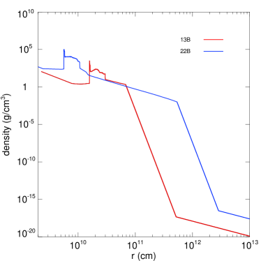
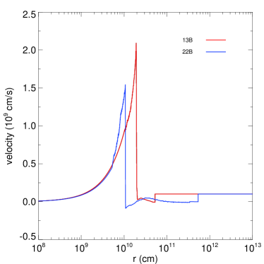
Figure 1.— Profiles for the shock, the star and its surrounding envelope as initialized in RAGE. Red: 13 foe HN, 25 ${M}_{\odot}$ progenitor. Blue: 22 foe HN, 50 ${M}_{\odot}$ progenitor. Left: densities. Right: velocities.

The expulsion of the envelope usually proceeds as an outburst that ejects a massive shell that is followed by a fast wind. If the shell is less than $\sim$ 0.01 pc from the star when it dies, ejecta from the HN will crash into it and make a superluminous Type IIn SN (e.g., Moriya et al., 2010, 2013; Whalen et al., 2013b). For simplicity, we assume that the shell has been driven beyond 1 pc so there is no collision and it is too diffuse to attenuate light from the explosion. We thus join a simple low-mass wind profile to the surface of the star:

$$\rho_{\mathrm{w}}(r)=\frac{\dot{m}}{4\pi r^{2}v_{\mathrm{w}}},\vspace{0.05in}$$ (1)

where $\dot{m}$ is the mass loss rate of the wind and $v_{\mathrm{w}}$ is its speed. We take $v_{\mathrm{w}}$ to be 1000 km s^-1 and the H and He mass fractions in the wind to be 76% and 24%, respectively. We choose $\dot{m}$ to yield $\rho_{\mathrm{w}}\sim$ 2 $\times$ 10^-18 g cm^-3 at the bottom of the density bridge from the surface of the star. This choice of wind ensures that it is optically thin at the bottom of the bridge but still dense enough to prevent numerical instabilities in the radiation solution there. The wind profile is continued along the grid until its density falls to $n=$ 0.1 cm^-3, that of the H II region of the star. The wind is then replaced by this uniform H II region. We show some initial density and velocity profiles for our RAGE models in Figure 1.

2.3. SPECTRUM

To calculate spectra from a RAGE blast profile we map its densities, temperatures, velocities and mass fractions onto a 2D grid in the Los Alamos SPECTRUM code. SPECTRUM then performs a direct sum of the luminosity of every fluid element in the discretized profile to compute the total flux escaping the ejecta along the line of sight at every wavelength. This procedure accounts for Doppler shifts and time dilation due to the relativistic expansion of the ejecta. SPECTRUM also calculates intensities of emission lines and the attenuation of flux along the line of sight, capturing both limb darkening and absorption lines imprinted on the flux by intervening material in the ejecta and wind. Each spectrum has 14899 wavelengths.

We first extract gas densities, velocities, mass fractions and radiation temperatures from the AMR hierarchy in RAGE and order them by radius. Because of constraints on machine memory and time, only a subset of these points are used in SPECTRUM. We determine the position of the radiation front, which is taken to be where $aT^{4}$ rises above 10^-4 erg/cm³. Next, we find the radius of the $\tau=$ 40 surface by integrating the optical depth due to Thomson scattering in from the outer boundary, taking $\kappa_{Th}$ to be 0.288 for H and He gas at the mass fractions in the wind (see Section 2.4 of Whalen et al., 2013e). This is the greatest depth from which most of the radiation can escape from the ejecta.

The extracted gas densities, velocities, temperatures and species mass fractions are then interpolated onto a 2D grid in $r$ and $\theta$ in SPECTRUM. The inner mesh boundary is the same as in RAGE and the outer boundary is 10¹⁸ cm. Eight hundred uniform zones in log $r$ are assigned from the center of the grid to the $\tau=$ 40 surface, and the region from the $\tau=$ 40 surface to the radiation front is partitioned into 6200 uniform zones in $r$. The wind between the front and the outer edge of the grid is divided into 500 uniform zones in log $r$, for a total of 7500 radial bins. The variables within each of these new radial bins are mass averaged so that the SPECTRUM profile reproduces very sharp features from the RAGE profile. The mesh is uniformly divided into 160 bins in $\mu=$ cos$\,\theta$ from -1 to 1.

Our grid fully resolves regions of the flow from which photons can escape the ejecta and only lightly samples those from which most cannot. We use a 2D grid in SPECTRUM even though our RAGE profiles are only 1D to approximate effects like limb darkening and P Cygni profiles. For example, photons approaching an observer from the leading edge of the fireball traverse different path lengths through the ejecta than those coming from the poles, and mapping to a 2D grid in SPECTRUM partially captures these effects on the overall luminosity reaching a distant point.

3. Blast Profiles

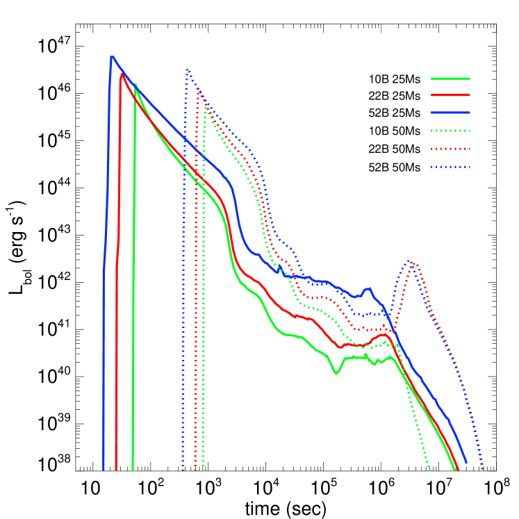
Figure 2.— Bolometric light curves for all six HNe.

Figure 3.— Hydrodynamic evolution of the 52 foe 50 ${M}_{\odot}$ Hn. Top: velocities; center: temperatures; bottom: densities. Left: shock breakout. From left to right the times are 342 s, 373 s, and 392 s. Center: intermediate evolution. From left to right, the times are 508 seconds, 800 seconds and 2508 seconds. Right: later evolution. From left to right, the times are 3.61 $\times$ 10⁴ seconds, 3.44 $\times$ 10⁵ seconds and 3.22 $\times$ 10⁶ seconds.

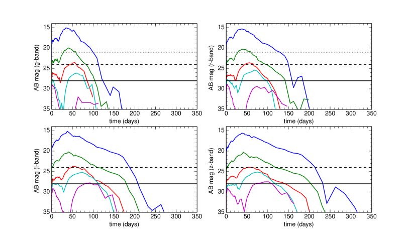
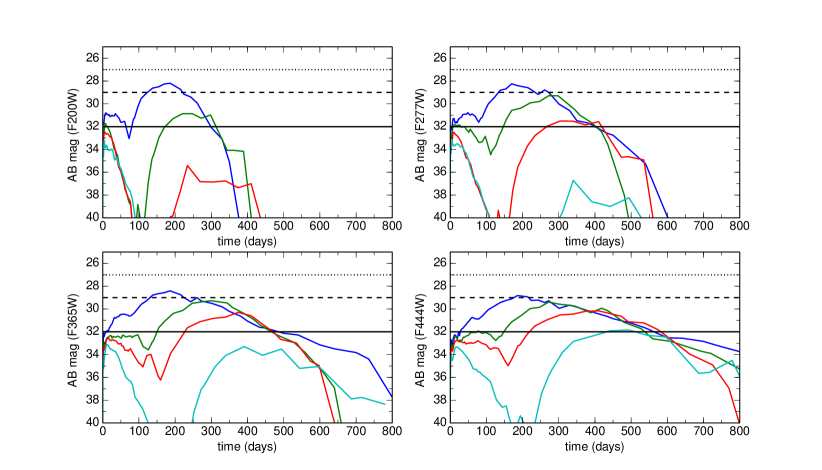
Figure 4.— Light curves for the 52 foe 50 ${M}_{\odot}$ HN at low redshifts (upper panels) and high redshifts (upper panels). In the upper panels, $z=$ 0.01 (dark blue), 0.1 (green), 0.5 (red), 1 (light blue), and 2 (purple). The horizontal dotted, dashed and solid lines are detection limits for PTF, Pan-STARRS and LSST, respectively. In the lower panels, $z=$ 4 (dark blue), 7 (green), 10 (red), 15 (light blue) and 20 (purple). The horizontal dotted, dashed and solid lines are detection limits for WFIRST, WFIRST with spectrum stacking and JWST, respectively. The wavelength of each filter can be read from its name; for example, the F277W filter is centered at 2.77 $\mu$m, and so forth.

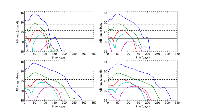
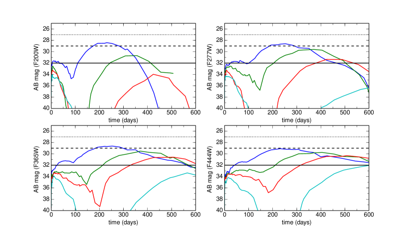
Figure 5.— Light curves for the 22 foe 50 ${M}_{\odot}$ HN at low redshifts (upper panels) and high redshifts (upper panels). In the upper panels, $z=$ 0.01 (dark blue), 0.1 (green), 0.5 (red), 1 (light blue), and 2 (purple). The horizontal dotted, dashed and solid lines are detection limits for PTF, Pan-STARRS and LSST, respectively. In the lower panels, $z=$ 4 (dark blue), 7 (green), 10 (red), 15 (light blue) and 20 (purple). The horizontal dotted, dashed and solid lines are detection limits for WFIRST, WFIRST with spectrum stacking and JWST, respectively. The wavelength of each filter can be read from its name; for example, the F277W filter is centered at 2.77 $\mu$m, and so forth.

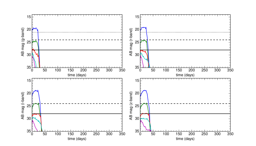
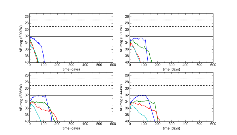
Figure 6.— Light curves for the 10 foe 50 ${M}_{\odot}$ HN at low redshifts (upper panels) and high redshifts (upper panels). In the upper panels, $z=$ 0.01 (dark blue), 0.1 (green), 0.5 (red), 1 (light blue), and 2 (purple). The horizontal dotted, dashed and solid lines are detection limits for PTF, Pan-STARRS and LSST, respectively. In the lower panels, $z=$ 4 (dark blue), 7 (green), 10 (red), 15 (light blue) and 20 (purple). The horizontal dotted, dashed and solid lines are detection limits for WFIRST, WFIRST with spectrum stacking and JWST, respectively. The wavelength of each filter can be read from its name; for example, the F277W filter is centered at 2.77 $\mu$m, and so forth.

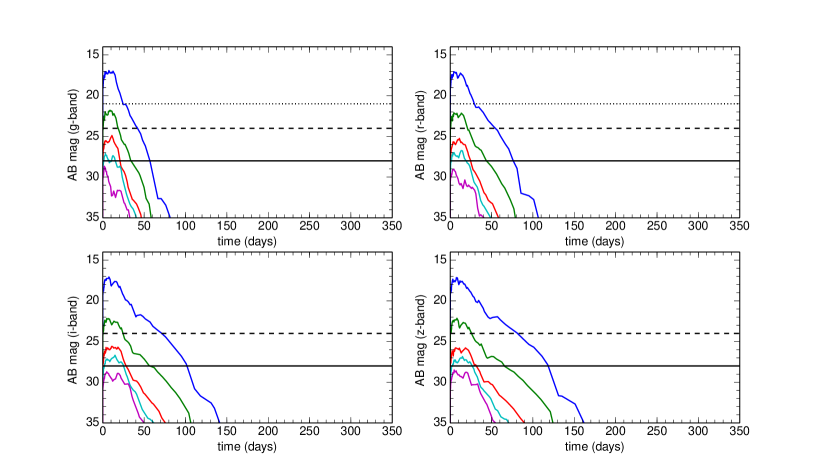
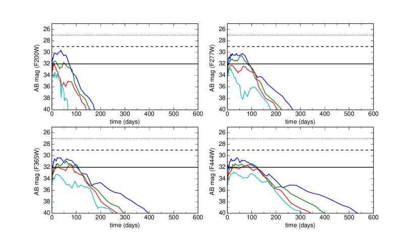
Figure 7.— Light curves for the 52 foe 25 ${M}_{\odot}$ HN at low redshifts (upper panels) and high redshifts (upper panels). In the upper panels, $z=$ 0.01 (dark blue), 0.1 (green), 0.5 (red), 1 (light blue), and 2 (purple). The horizontal dotted, dashed and solid lines are detection limits for PTF, Pan-STARRS and LSST, respectively. In the lower panels, $z=$ 4 (dark blue), 7 (green), 10 (red), 15 (light blue) and 20 (purple). The horizontal dotted, dashed and solid lines are detection limits for WFIRST, WFIRST with spectrum stacking and JWST, respectively. The wavelength of each filter can be read from its name; for example, the F277W filter is centered at 2.77 $\mu$m, and so forth.

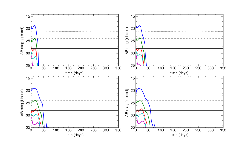
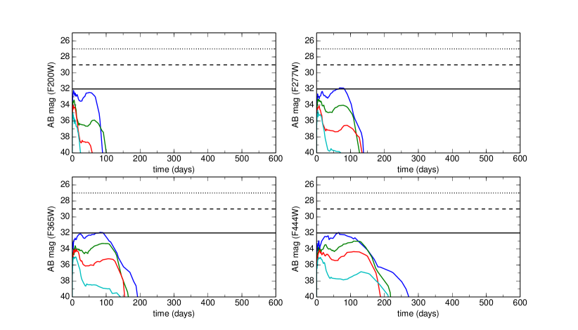
Figure 8.— Light curves for the 22 foe 25 ${M}_{\odot}$ HN at low redshifts (upper panels) and high redshifts (upper panels). In the upper panels, $z=$ 0.01 (dark blue), 0.1 (green), 0.5 (red), 1 (light blue), and 2 (purple). The horizontal dotted, dashed and solid lines are detection limits for PTF, Pan-STARRS and LSST, respectively. In the lower panels, $z=$ 4 (dark blue), 7 (green), 10 (red), 15 (light blue) and 20 (purple). The horizontal dotted, dashed and solid lines are detection limits for WFIRST, WFIRST with spectrum stacking and JWST, respectively. The wavelength of each filter can be read from its name; for example, the F277W filter is centered at 2.77 $\mu$m, and so forth.

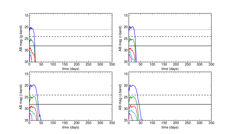
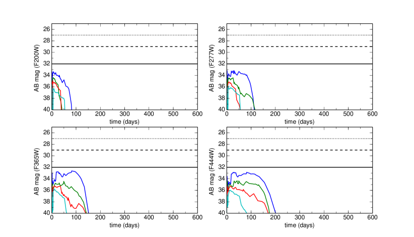
Figure 9.— Light curves for the 10 foe 25 ${M}_{\odot}$ HN at low redshifts (upper panels) and high redshifts (upper panels). In the upper panels, $z=$ 0.01 (dark blue), 0.1 (green), 0.5 (red), 1 (light blue), and 2 (purple). The horizontal dotted, dashed and solid lines are detection limits for PTF, Pan-STARRS and LSST, respectively. In the lower panels, $z=$ 4 (dark blue), 7 (green), 10 (red), 15 (light blue) and 20 (purple). The horizontal dotted, dashed and solid lines are detection limits for WFIRST, WFIRST with spectrum stacking and JWST, respectively. The wavelength of each filter can be read from its name; for example, the F277W filter is centered at 2.77 $\mu$m, and so forth.

We show bolometric luminosities for all six HNe in Figure 2 and hydro profiles for the 52 foe 50 ${M}_{\odot}$ HN in Figure 3. We first examine shock breakout from the star, as shown in the left column of Figure 3. After breakout, the radiation pulse from the shock blows the outer layers of the star outward at $\sim$ 2.4 $\times$ 10¹⁰ cm s^-1 as it descends the density bridge. This radiative precursor stops accelerating as it reaches the bottom of the bridge. Radiation breakout coincides with shock breakout. The radiation front (the temperature plateau at 373 and 392 seconds) initially heats the gas to $\sim$ 200 eV. As the fireball expands, it cools by emitting photons and performing $PdV$ work on the envelope. As it cools, its spectrum softens, and the temperature to which the radiation front heats the surrounding gas also falls.

Naively, one might expect the duration of the breakout transient to be roughly the light crossing time of the star. It is actually longer in part because photons remain partially coupled to the wispy outer layers of the star that are blown off by the breakout pulse. As they diffuse out through this radiative precursor, they broaden the transient. Also, the opacities are frequency dependent, and photons break free of the flow at different times at different wavelengths. This effect also broadens the pulse in time (Bayless et al., 2014). A few seconds after the precursor is blown off from the shock, at $\sim$ 390 seconds, photons escape from its outer layers and become visible to an external observer. As shown in Figure 2, the bolometric luminosity of the breakout transient varies from $\sim$ 10⁴⁶ to 10⁴⁷ erg s^-1 and increases with explosion energy for a given stellar mass. The transient is dimmer in more massive SNe at a given energy because of the greater inertia of the ejecta.

Shock breakout happens earlier in the less massive star at a given energy because of its smaller radius. It happens earlier at higher energies because the shock reaches the surface sooner. The breakout transient is composed mostly of X-rays and hard UV. At $z\sim 20$ the transient would would last up to 1 - 2 days today, in principle making it much easier to detect at this redshift than in the local universe. But while it is the most luminous phase of the SN, shock breakout is least visible at high redshifts due to absorption by the neutral IGM. Whatever X-rays that are not absorbed would redshifted into the far UV and stopped by the outer layers of our Galaxy.

Radiation from the shock sustains the radiative precursor until $\sim$ 2500 seconds, as shown in the center column of Figure 3. The precursor is visible as the slightly noisy ramp in density between the shock and the surrounding wind at 3 $\times$ 10¹² cm at 508 seconds. It is also visible in the break in the velocity peak at the same position and time. The shock soon overtakes the precursor and merges with it because it dims as it expands and cools, so its radiative flux can no longer maintain it.

The rebrightening in the 22 and 52 foe explosions at $\sim$ 5 $\times 10^{5}$ s to $10^{7}$ s is due to the decay of ${}^{56}\mathrm{Ni}$ in the ejecta. It is brighter with greater explosion energy at a given progenitor mass because more ${}^{56}\mathrm{Ni}$ is synthesized, and it is absent in the least energetic 25 ${M}_{\odot}$ and 50 ${M}_{\odot}$ HNe because they make very little ${}^{56}\mathrm{Ni}$. Rebrightening happens sooner with the 25 ${M}_{\odot}$ progenitor because of the shorter radiation diffusion timescales in the ejecta. We note that the expansion of the flow is nearly homologous after 10⁴ seconds except for internal expansion of the ${}^{56}\mathrm{Ni}$ bubble relative to the surrounding ejecta due to decay heating. All six HNe evolve through similar stages.

4. NIR Light Curves / Detection Limits

NIR observations are required to detect SNe before the end of reionization ($z\sim$ 6) because flux blueward of the Lyman limit at higher redshifts is absorbed by the neutral IGM. This also limits detections of such events in the optical to $z<$ 6. All-sky surveys are probably the best prospects for detecting large numbers of high $z$ SNe because their large survey areas can compensate for low star formation rates (SFRs) at early epochs (e.g., Fig. 3 of Whalen et al., 2013h). But even 30-m class telescopes with narrow fields of view such as JWST, the Giant Magellan Telescope (GMT), the Thirty-Meter Telescope (TMT), and the European Extremely Large Telescope (E-ELT) are still expected to find appreciable numbers of Pop III SNe (Hummel et al., 2012). We now consider detection limits in redshift for our HNe in the NIR for explosions at $z>$ 6 and in the optical for events below this redshift.

In Figures 4-9, we show visible and NIR light curves for all six HNe along with detection limits for current and proposed instruments for $z=$ 0.01 - 20. They were obtained from the spectra by summing their luminosities over the appropriate bands and then cosmologically redshifting and dimming them. Since the NIR light curves are all redward of the Lyman limit in the frame of the explosion, we take the transmission coefficient of the neutral IGM at $z\gtrsim$ 6 to be 1 (see Figure 3 of de Souza et al., 2013). The detection limits for the Palomar Transient Factory (PTF), the Panoramic Survey Telescope & Rapid Response System (Pan-STARRS) and the Large Synoptic Survey Telescope (LSST) are AB mag 21, 24 and 28, respectively. Photometry limits for JWST and WFIRST are AB mag 32 and 27, respectively, which could be extended to 29 for WFIRST with spectrum stacking. Note that wavelengths can be extracted from the JWST filter names by dividing their numbers by 100, i.e., the F277W is for 2.77 $\mu$m.

The NIR light curves of the most energetic 50 ${M}_{\odot}$ HNe exhibit a initial, short-lived peak corresponding to the post-breakout expansion and cooling of the fireball followed by a second brighter and much longer peak due to ${}^{56}\mathrm{Ni}$ rebrightening. JWST detections of the dimmest 50 ${M}_{\odot}$ HNe will be restricted to $z\lesssim$ 4, but the more energetic ones will be visible out to $z=$ 10 - 15. The most energetic 25 ${M}_{\odot}$ Hn will only be visible to JWST out to $z\sim$ 4 - 7. WFIRST will only observe the brightest HNe out to $z\sim$ 4 - 5. While JWST could therefore detect Pop III HNe in primordial galaxies if it happened across one, WFIRST in principle could see many more of these events, but only out to the end of cosmological reionization. The fact that these SNe rise above photometry limits in multiple filters at a given redshift makes it easier to identify them as transients.

The 22 and 52 foe 50 ${M}_{\odot}$ explosions will be visible to PTF out to $z\sim$ 0.01 - 0.1, to Pan-STARRS out to $z\sim$ 0.1 - 0.5, and to LSST out to $z\sim$ 1 - 2. The 10 foe HN will be visible to PTF out to $z\sim$ 0.01, to Pan-STARRS out to $z\sim$ 0.01 - 0.1, and to LSST out to $z\sim$ 0.1 - 0.5. The 25 ${M}_{\odot}$ HNe as a rule are significantly dimmer and less long-lived than the 50 ${M}_{\odot}$ HNe. The 25 ${M}_{\odot}$ explosions will be visible to PTF out to $z\sim$ 0.01. Pan-STARRS will detect these events out to $z\sim$ 0.01 - 0.1. LSST will observe these HNe out to $z\sim$ 0.5 - 1, with most events being limited to $z\lesssim$ 0.5.

5. Pop III HN Rates

Pop III HN rates are uncertain because the primordial IMF and star formation rates are unknown. But there is reason to believe that Pop III stars end their lives as HNe at high enough rates to be detected in future surveys. Today, the observed HN rate is within a factor of a few of the GRB rate, which is not surprising given that both are associated with Type Ib/c SNe whose progenitors are probably rapidly-rotating stars with masses $\gtrsim$ 30 ${M}_{\odot}$ (Podsiadlowski et al., 2004; Guetta & Della Valle, 2007). Most Pop III stars are at least this massive, and many of them may be born with high rotation rates (Stacy et al., 2011, 2013; Maeder & Meynet, 2012) and die as GRBs or HNe more often than do stars of similar mass today (e.g., Yoon & Langer, 2005; Hirschi et al., 2005; Woosley & Heger, 2006; Nagakura et al., 2012; Yoon et al., 2012)). There is also evidence that rapidly-rotating Pop III stars (Chiappini et al., 2011) and perhaps HNe (Nomoto et al., 2010) may have synthesized the heavy elements detected in metal-poor stars, which also suggests that HNe may have been common among early stars.

If Pop III HN rates also trace the GRB rate, several recent estimates of the Pop III GRB rate can be used to derive the Pop III HN rate. Bromm & Loeb (2006) predict a total rate of observed Pop III GRBs of $\sim$ 0.1 yr^-1 at $z\gtrsim$ 15, which would correspond to $\gtrsim$ 10 HNe yr^-1 if they can be seen at any viewing angle (i.e., if the beaming factor used to calculate the GRB rate is divided out). Distinguishing between Pop III stars that are formed with and without radiative feedback during early galaxy formation, de Souza et al. (2011) predict that GRBs from the former are orders of magnitude more common than those from the latter. They predict an intrinsic GRB rate of $\gtrsim$ 100 yr^-1 out to $z$ $\sim$ 15. Campisi et al. (2011) use cosmological simulations of metal enrichment and Pop III and II star formation to place an upper limit of $\sim$ 1 yr^-1 on the observed Pop III GRB rate at $z$ $>$ 6, or about 100 HNe yr^-1.

Even if no connection is assumed for Pop III GRBs and HNe, an upper limit to the HN rate can be gleaned from cosmological simulations of Pop III star formation that include chemical and radiative feedback (Johnson et al., 2013a) by assuming that all 25 - 140 ${M}_{\odot}$ Pop III stars can produce black holes and HNe (e.g., Fryer, 1999; Heger et al., 2003). Assuming a Salpeter-like IMF for primordial stars and a lower mass limit of 21 ${M}_{\odot}$, Johnson et al. (2013a) find a total HN rate of $\sim$ 10⁴ yr^-1, with most occurring at $z$ $\lesssim$ 10. This rate is broadly consistent with the estimates above if the actual ratio of Pop III black hole-producing SNe to Pop III HNe is similar to the observed ratio today ($\sim$ 100; Podsiadlowski et al., 2004). We conclude that HNe could occur at rates of $\gtrsim$ 10 yr^-1, and perhaps up to $\gtrsim$ 100 yr^-1, at $z$ $\lesssim$ 15.

6. Conclusion

Pop III HNe will be visible in the NIR out to $z\sim$ 10 - 15 by JWST and out to $z\sim$ 4 - 5 to WFIRST and WISH. These redshifts would go up dramatically if the HN crashes into a massive shell ejected by the progenitor. Such collisions can produce superluminous supernovae (SLSNe) like SN 2006gy (Smith et al., 2007; Moriya et al., 2010; Chevalier & Irwin, 2011; Moriya et al., 2013) that would be brighter than the HN itself. The high luminosities of SLSNe are due to the large radius of the shell upon impact. Much less energetic Pop III Type IIn SNe (2 foe) can be detected by JWST at $z\sim$ 15 - 20 and WFIRST at $z\sim$ 7 (Whalen et al., 2013b), so HNe that collide with dense shells may be visible to all-sky NIR missions like WFIRST out to $z\sim$ 10 - 15. This would greatly enhance their prospects for detection, since the large survey areas of these missions could compensate for low HN rates. We are now modeling these events with RAGE.

The ejection of the H layer prior to the HN could create a dense wind rather than a shell, and this envelope could also affect the luminosity of the explosion (Bayless et al., 2014). When the shock crashes into this wind it could become even hotter, and thus more luminous. But more of this luminosity may also be absorbed by the envelope downwind of the shock. Additional simulations are required to determine the overall effect of dense envelopes on the luminosity of the HN. We considered only HNe in very diffuse winds, in which all vestiges of the H layer are driven beyond the immediate reach of the ejecta, as a simplest case.

Many of the HNe detected by JWST at $z\sim$ 10 - 15 could be zero-metallicity events, especially in cases where supersonic baryonic streaming motion delays first star formation to $z\sim$ 15 - 17 (Tseliakhovich & Hirata, 2010; Greif et al., 2011b). But HNe found by WFIRST at $z\sim$ 4 - 5 would probably not be Pop III explosions, even though Trenti et al. (2009) have found that Pop III star formation could extend down to $z\sim$ 6, and large pockets of metal-free gas have now been discovered at $z\sim$ 2 (Fumagalli et al., 2011). How might HNe at $Z\sim$ 0.1 $Z_{\odot}$ differ from Pop III events? It has been found that the central engines of core-collapse explosions do not vary strongly with metallicity because the cores of $Z=$ 0 and $Z_{\odot}$ stars have similar entropy profiles (Chieffi & Limongi, 2004; Woosley & Heger, 2007) (see also Figure 1 of Whalen & Fryer, 2012). It is therefore likely that HNe at the end of reionization would have similar energies to those in the primordial universe.

Although we have modeled Pop III HNe with 1D simulations, they are inherently multidimensional events because of their highly asymmetric central engines. Real HNe may therefore exhibit azimuthally-dependent luminosities that could affect not only their detection limits in the NIR at high redshift but how many of these events would actually be seen for a given opening angle for the engine. Future 2D radiation hydrodynamical simulations could address these issues. But for now, as with other studies (Moriya et al., 2013), we must rely on 1D models to estimate the NIR signatures of these events. Because our simulations are 1D, they also neglect mixing during the explosion. Mixing could have some impact on the luminosity if it dredges up ${}^{56}\mathrm{Ni}$ from greater depths during the explosion. Mixing can also affect the order in which lines appear in the spectra over time.

If most Pop III HNe are associated with GRBs, and most GRBs are due to binary mergers with companion stars (e.g., Fryer & Woosley, 1998; Fryer et al., 1999b; Zhang & Fryer, 2001; Fryer et al., 2007), then there is additional reason to believe HNe may have been common in the primordial universe because Pop III stars have now been found to form in binaries and small multiples in simulations (Turk et al., 2009; Stacy et al., 2010). The GRBs themselves might be detected by other means. Gamma rays from these events could trigger Swift or its successors, such as the Joint Astrophysics Nascent Universe Satellite (JANUS, Mészáros & Rees, 2010; Roming, 2008; Burrows et al., 2010), and their afterglows (Whalen et al., 2008b) might be found in all-sky radio surveys by the Extended Very Large Array (eVLA), eMERLIN and the Square Kilometer Array (SKA) (de Souza et al., 2011) (see also Suwa & Ioka, 2011; Nagakura et al., 2012). It is now known that Pop III GRB afterglows will be bright enough in the NIR to be seen JWST, WFIRST, and the TMT (Mesler et al., 2012, 2014) (and that they would completely outshine the HN).

Could later stages of HNe be detected in other ways? Whalen et al. (2008c) found that most of the kinetic energy of 40 ${M}_{\odot}$ Pop III HNe is eventually radiated away as H and He lines in primordial halos as the remnant sweeps up and shocks gas. This emission is too diffuse, redshifted and extended over time to be detected by any upcoming instruments. Also, unlike Pop III PI SNe, HNe do not inject enough energy into the cosmic microwave background (CMB) to impose excess power on the CMB at small scales (Oh et al., 2003; Whalen et al., 2008c) or be directly imaged by the Atacama Cosmology Telescope or the South Pole Telescope via the Sunyaev-Zeldovich effect. But new calculations reveal that enough synchrotron emission from their remnants would redshifted into the radio above $z\sim$ 10 to be directly detected by current facilities such as eVLA and eMERLIN and by SKA (Meiksin & Whalen, 2013). Whether in the NIR, radio, or in the fossil abundance record, these ancient explosions could soon open another window on the $z\sim$ 10 - 15 universe.

References

- Agarwal et al. (2012) Agarwal, B., Khochfar, S., Johnson, J. L., Neistein, E., Dalla Vecchia, C., & Livio, M. 2012, MNRAS, 425, 2854
- Almgren et al. (2010) Almgren, A. S., Beckner, V. E., Bell, J. B., Day, M. S., Howell, L. H., Joggerst, C. C., Lijewski, M. J., Nonaka, A., Singer, M., & Zingale, M. 2010, ApJ, 715, 1221
- Alvarez et al. (2009) Alvarez, M. A., Wise, J. H., & Abel, T. 2009, ApJ, 701, L133
- Baraffe et al. (2001) Baraffe, I., Heger, A., & Woosley, S. E. 2001, ApJ, 550, 890
- Bayless et al. (2014) Bayless, A. J., Even, W., Frey, L. H., Fryer, C. L., Roming, P. W. A., & Young, P. A. 2014, arXiv:1401.4449
- Beers & Christlieb (2005) Beers, T. C. & Christlieb, N. 2005, ARA&A, 43, 531
- Benz et al. (1989) Benz, W., Thielemann, F.-K., & Hills, J. G. 1989, ApJ, 342, 986
- Bromm & Loeb (2006) Bromm, V. & Loeb, A. 2006, ApJ, 642, 382
- Burrows et al. (2010) Burrows, D. N., Roming, P. W. A., Fox, D. B., Herter, T. L., Falcone, A., Bilén, S., Nousek, J. A., & Kennea, J. A. 2010, in Presented at the Society of Photo-Optical Instrumentation Engineers (SPIE) Conference, Vol. 7732, Society of Photo-Optical Instrumentation Engineers (SPIE) Conference Series
- Campisi et al. (2011) Campisi, M. A., Maio, U., Salvaterra, R., & Ciardi, B. 2011, MNRAS, 416, 2760
- Chatzopoulos & Wheeler (2012) Chatzopoulos, E. & Wheeler, J. C. 2012, ApJ, 748, 42
- Chatzopoulos et al. (2013) Chatzopoulos, E., Wheeler, J. C., & Couch, S. M. 2013, ApJ, 776, 129
- Chen et al. (2014a) Chen, K.-J., Heger, A., Woosley, S., Almgren, A., & Whalen, D. J. 2014a, ApJ, 792, 44
- Chen et al. (2014b) Chen, K.-J., Heger, A., Woosley, S., Almgren, A., Whalen, D. J., & Johnson, J. L. 2014b, ApJ, 790, 162
- Chen et al. (2014c) Chen, K.-J., Woosley, S., Heger, A., Almgren, A., & Whalen, D. J. 2014c, ApJ, 792, 28
- Chevalier & Irwin (2011) Chevalier, R. A. & Irwin, C. M. 2011, ApJ, 729, L6+
- Chiappini et al. (2011) Chiappini, C., Frischknecht, U., Meynet, G., Hirschi, R., Barbuy, B., Pignatari, M., Decressin, T., & Maeder, A. 2011, Nature, 474, 666
- Chieffi & Limongi (2004) Chieffi, A. & Limongi, M. 2004, ApJ, 608, 405
- Clark et al. (2011) Clark, P. C., Glover, S. C. O., Smith, R. J., Greif, T. H., Klessen, R. S., & Bromm, V. 2011, Science, 331, 1040
- Cooke et al. (2012) Cooke, J., Sullivan, M., Gal-Yam, A., Barton, E. J., Carlberg, R. G., Ryan-Weber, E. V., Horst, C., Omori, Y., & Díaz, C. G. 2012, Nature, 491, 228
- de Souza et al. (2013) de Souza, R. S., Ishida, E. E. O., Johnson, J. L., Whalen, D. J., & Mesinger, A. 2013, MNRAS, 436, 1555
- de Souza et al. (2014) de Souza, R. S., Ishida, E. E. O., Whalen, D. J., Johnson, J. L., & Ferrara, A. 2014, MNRAS, 442, 1640
- de Souza et al. (2011) de Souza, R. S., Yoshida, N., & Ioka, K. 2011, A&A, 533, A32
- Ekström et al. (2008) Ekström, S., Meynet, G., Chiappini, C., Hirschi, R., & Maeder, A. 2008, A&A, 489, 685
- Frebel et al. (2005) Frebel, A., Aoki, W., Christlieb, N., Ando, H., Asplund, M., Barklem, P. S., Beers, T. C., Eriksson, K., Fechner, C., Fujimoto, M. Y., Honda, S., Kajino, T., Minezaki, T., Nomoto, K., Norris, J. E., Ryan, S. G., Takada-Hidai, M., Tsangarides, S., & Yoshii, Y. 2005, Nature, 434, 871
- Frey et al. (2013) Frey, L. H., Even, W., Whalen, D. J., Fryer, C. L., Hungerford, A. L., Fontes, C. J., & Colgan, J. 2013, ApJS, 204, 16
- Fryer et al. (1999a) Fryer, C., Benz, W., Herant, M., & Colgate, S. A. 1999a, ApJ, 516, 892
- Fryer (1999) Fryer, C. L. 1999, ApJ, 522, 413
- Fryer et al. (2009) Fryer, C. L., Brown, P. J., Bufano, F., Dahl, J. A., Fontes, C. J., Frey, L. H., Holland, S. T., Hungerford, A. L., Immler, S., Mazzali, P., Milne, P. A., Scannapieco, E., Weinberg, N., & Young, P. A. 2009, ApJ, 707, 193
- Fryer et al. (2007) Fryer, C. L., Mazzali, P. A., Prochaska, J., Cappellaro, E., Panaitescu, A., Berger, E., van Putten, M., van den Heuvel, E. P. J., Young, P., Hungerford, A., Rockefeller, G., Yoon, S.-C., Podsiadlowski, P., Nomoto, K., Chevalier, R., Schmidt, B., & Kulkarni, S. 2007, PASP, 119, 1211
- Fryer et al. (2006) Fryer, C. L., Rockefeller, G., & Young, P. A. 2006, ApJ, 647, 1269
- Fryer et al. (2010) Fryer, C. L., Whalen, D. J., & Frey, L. 2010, in American Institute of Physics Conference Series, Vol. 1294, American Institute of Physics Conference Series, ed. D. J. Whalen, V. Bromm, & N. Yoshida, 70–75
- Fryer & Woosley (1998) Fryer, C. L. & Woosley, S. E. 1998, ApJ, 502, L9
- Fryer et al. (1999b) Fryer, C. L., Woosley, S. E., & Hartmann, D. H. 1999b, ApJ, 526, 152
- Fumagalli et al. (2011) Fumagalli, M., O’Meara, J. M., & Prochaska, J. X. 2011, Science, 334, 1245
- Gal-Yam et al. (2009) Gal-Yam, A., Mazzali, P., Ofek, E. O., Nugent, P. E., Kulkarni, S. R., Kasliwal, M. M., Quimby, R. M., Filippenko, A. V., Cenko, S. B., Chornock, R., Waldman, R., Kasen, D., Sullivan, M., Beshore, E. C., Drake, A. J., Thomas, R. C., Bloom, J. S., Poznanski, D., Miller, A. A., Foley, R. J., Silverman, J. M., Arcavi, I., Ellis, R. S., & Deng, J. 2009, Nature, 462, 624
- Gardner et al. (2006) Gardner, J. P., Mather, J. C., Clampin, M., Doyon, R., Greenhouse, M. A., Hammel, H. B., Hutchings, J. B., Jakobsen, P., Lilly, S. J., Long, K. S., Lunine, J. I., McCaughrean, M. J., Mountain, M., Nella, J., Rieke, G. H., Rieke, M. J., Rix, H.-W., Smith, E. P., Sonneborn, G., Stiavelli, M., Stockman, H. S., Windhorst, R. A., & Wright, G. S. 2006, Space Sci. Rev., 123, 485
- Gittings et al. (2008) Gittings, M., Weaver, R., Clover, M., Betlach, T., Byrne, N., Coker, R., Dendy, E., Hueckstaedt, R., New, K., Oakes, W. R., Ranta, D., & Stefan, R. 2008, Computational Science and Discovery, 1, 015005
- Glover (2013) Glover, S. 2013, in Astrophysics and Space Science Library, Vol. 396, Astrophysics and Space Science Library, ed. T. Wiklind, B. Mobasher, & V. Bromm, 103
- Greif et al. (2012) Greif, T. H., Bromm, V., Clark, P. C., Glover, S. C. O., Smith, R. J., Klessen, R. S., Yoshida, N., & Springel, V. 2012, MNRAS, 424, 399
- Greif et al. (2010) Greif, T. H., Glover, S. C. O., Bromm, V., & Klessen, R. S. 2010, ApJ, 716, 510
- Greif et al. (2011a) Greif, T. H., Springel, V., White, S. D. M., Glover, S. C. O., Clark, P. C., Smith, R. J., Klessen, R. S., & Bromm, V. 2011a, ApJ, 737, 75
- Greif et al. (2011b) Greif, T. H., White, S. D. M., Klessen, R. S., & Springel, V. 2011b, ApJ, 736, 147
- Guetta & Della Valle (2007) Guetta, D. & Della Valle, M. 2007, ApJ, 657, L73
- Heger et al. (2003) Heger, A., Fryer, C. L., Woosley, S. E., Langer, N., & Hartmann, D. H. 2003, ApJ, 591, 288
- Heger & Woosley (2002) Heger, A. & Woosley, S. E. 2002, ApJ, 567, 532
- Herant et al. (1994) Herant, M., Benz, W., Hix, W. R., Fryer, C. L., & Colgate, S. A. 1994, ApJ, 435, 339
- Hirano et al. (2014) Hirano, S., Hosokawa, T., Yoshida, N., Umeda, H., Omukai, K., Chiaki, G., & Yorke, H. W. 2014, ApJ, 781, 60
- Hirschi et al. (2005) Hirschi, R., Meynet, G., & Maeder, A. 2005, A&A, 443, 581
- Hosokawa et al. (2011) Hosokawa, T., Omukai, K., Yoshida, N., & Yorke, H. W. 2011, Science, 334, 1250
- Hummel et al. (2012) Hummel, J. A., Pawlik, A. H., Milosavljević, M., & Bromm, V. 2012, ApJ, 755, 72
- Iwamoto et al. (1998) Iwamoto, K., Mazzali, P. A., Nomoto, K., Umeda, H., Nakamura, T., Patat, F., Danziger, I. J., Young, T. R., Suzuki, T., Shigeyama, T., Augusteijn, T., Doublier, V., Gonzalez, J.-F., Boehnhardt, H., Brewer, J., Hainaut, O. R., Lidman, C., Leibundgut, B., Cappellaro, E., Turatto, M., Galama, T. J., Vreeswijk, P. M., Kouveliotou, C., van Paradijs, J., Pian, E., Palazzi, E., & Frontera, F. 1998, Nature, 395, 672
- Iwamoto et al. (2005) Iwamoto, N., Umeda, H., Tominaga, N., Nomoto, K., & Maeda, K. 2005, Science, 309, 451
- Jeon et al. (2012) Jeon, M., Pawlik, A. H., Greif, T. H., Glover, S. C. O., Bromm, V., Milosavljević, M., & Klessen, R. S. 2012, ApJ, 754, 34
- Joggerst et al. (2010) Joggerst, C. C., Almgren, A., Bell, J., Heger, A., Whalen, D., & Woosley, S. E. 2010, ApJ, 709, 11
- Joggerst & Whalen (2011) Joggerst, C. C. & Whalen, D. J. 2011, ApJ, 728, 129
- Johnson et al. (2013a) Johnson, J. L., Dalla, V. C., & Khochfar, S. 2013a, MNRAS, 428, 1857
- Johnson et al. (2009) Johnson, J. L., Greif, T. H., Bromm, V., Klessen, R. S., & Ippolito, J. 2009, MNRAS, 399, 37
- Johnson et al. (2014) Johnson, J. L., Whalen, D. J., Agarwal, B., Paardekooper, J.-P., & Khochfar, S. 2014, arXiv:1405.2081
- Johnson et al. (2013b) Johnson, J. L., Whalen, D. J., Even, W., Fryer, C. L., Heger, A., Smidt, J., & Chen, K.-J. 2013b, ApJ, 775, 107
- Johnson et al. (2012) Johnson, J. L., Whalen, D. J., Fryer, C. L., & Li, H. 2012, ApJ, 750, 66
- Johnson et al. (2013c) Johnson, J. L., Whalen, D. J., Li, H., & Holz, D. E. 2013c, ApJ, 771, 116
- Kasen et al. (2011) Kasen, D., Woosley, S. E., & Heger, A. 2011, ApJ, 734, 102
- Kudritzki (2000) Kudritzki, R. 2000, in The First Stars, ed. A. Weiss, T. G. Abel, & V. Hill, 127–+
- Latif et al. (2013a) Latif, M. A., Schleicher, D. R. G., Schmidt, W., & Niemeyer, J. 2013a, MNRAS, 433, 1607
- Latif et al. (2013b) —. 2013b, MNRAS, 430, 588
- Löhner (1987) Löhner, R. 1987, Comput. Methods Appl. Mech. Eng., 61, 323
- Mackey et al. (2003) Mackey, J., Bromm, V., & Hernquist, L. 2003, ApJ, 586, 1
- Maeda & Nomoto (2003) Maeda, K. & Nomoto, K. 2003, ApJ, 598, 1163
- Maeder & Meynet (2012) Maeder, A. & Meynet, G. 2012, Reviews of Modern Physics, 84, 25
- Magee et al. (1995) Magee, N. H., Abdallah, Jr., J., Clark, R. E. H., Cohen, J. S., Collins, L. A., Csanak, G., Fontes, C. J., Gauger, A., Keady, J. J., Kilcrease, D. P., & Merts, A. L. 1995, in Astronomical Society of the Pacific Conference Series, Vol. 78, Astrophysical Applications of Powerful New Databases, ed. S. J. Adelman & W. L. Wiese, 51
- Mazzali et al. (2008) Mazzali, P. A., Valenti, S., Della Valle, M., Chincarini, G., Sauer, D. N., Benetti, S., Pian, E., Piran, T., D’Elia, V., Elias-Rosa, N., Margutti, R., Pasotti, F., Antonelli, L. A., Bufano, F., Campana, S., Cappellaro, E., Covino, S., D’Avanzo, P., Fiore, F., Fugazza, D., Gilmozzi, R., Hunter, D., Maguire, K., Maiorano, E., Marziani, P., Masetti, N., Mirabel, F., Navasardyan, H., Nomoto, K., Palazzi, E., Pastorello, A., Panagia, N., Pellizza, L. J., Sari, R., Smartt, S., Tagliaferri, G., Tanaka, M., Taubenberger, S., Tominaga, N., Trundle, C., & Turatto, M. 2008, Science, 321, 1185
- Meiksin & Whalen (2013) Meiksin, A. & Whalen, D. J. 2013, MNRAS, 430, 2854
- Mesler et al. (2012) Mesler, R. A., Whalen, D. J., Lloyd-Ronning, N. M., Fryer, C. L., & Pihlström, Y. M. 2012, ApJ, 757, 117
- Mesler et al. (2014) Mesler, R. A., Whalen, D. J., Smidt, J., Fryer, C. L., Lloyd-Ronning, N. M., & Pihlström, Y. M. 2014, ApJ, 787, 91
- Mészáros & Rees (2010) Mészáros, P. & Rees, M. J. 2010, ApJ, 715, 967
- Milosavljević et al. (2009) Milosavljević, M., Bromm, V., Couch, S. M., & Oh, S. P. 2009, ApJ, 698, 766
- Moriya et al. (2010) Moriya, T., Yoshida, N., Tominaga, N., Blinnikov, S. I., Maeda, K., Tanaka, M., & Nomoto, K. 2010, in American Institute of Physics Conference Series, Vol. 1294, American Institute of Physics Conference Series, ed. D. J. Whalen, V. Bromm, & N. Yoshida, 268–269
- Moriya et al. (2013) Moriya, T. J., Blinnikov, S. I., Tominaga, N., Yoshida, N., Tanaka, M., Maeda, K., & Nomoto, K. 2013, MNRAS, 428, 1020
- Nagakura et al. (2012) Nagakura, H., Suwa, Y., & Ioka, K. 2012, ApJ, 754, 85
- Nakamura et al. (2001) Nakamura, T., Mazzali, P. A., Nomoto, K., & Iwamoto, K. 2001, ApJ, 550, 991
- Nomoto et al. (2001) Nomoto, K., Mazzali, P. A., Nakamura, T., Iwamoto, K., Danziger, I. J., & Patat, F. 2001, in Supernovae and Gamma-Ray Bursts: the Greatest Explosions since the Big Bang, ed. M. Livio, N. Panagia, & K. Sahu, 144–170
- Nomoto et al. (2010) Nomoto, K., Tanaka, M., Tominaga, N., & Maeda, K. 2010, New Astronomy Reviews, 54, 191
- Oh et al. (2003) Oh, S. P., Cooray, A., & Kamionkowski, M. 2003, MNRAS, 342, L20
- O’Shea et al. (2005) O’Shea, B. W., Abel, T., Whalen, D., & Norman, M. L. 2005, ApJ, 628, L5
- O’Shea & Norman (2007) O’Shea, B. W. & Norman, M. L. 2007, ApJ, 654, 66
- Pan et al. (2012a) Pan, T., Kasen, D., & Loeb, A. 2012a, MNRAS, 422, 2701
- Pan et al. (2012b) Pan, T., Loeb, A., & Kasen, D. 2012b, MNRAS, 423, 2203
- Park & Ricotti (2011) Park, K. & Ricotti, M. 2011, ApJ, 739, 2
- Pawlik et al. (2011) Pawlik, A. H., Milosavljević, M., & Bromm, V. 2011, ApJ, 731, 54
- Pawlik et al. (2013) —. 2013, ApJ, 767, 59
- Podsiadlowski et al. (2004) Podsiadlowski, P., Mazzali, P. A., Nomoto, K., Lazzati, D., & Cappellaro, E. 2004, ApJ, 607, L17
- Ritter et al. (2012) Ritter, J. S., Safranek-Shrader, C., Gnat, O., Milosavljević, M., & Bromm, V. 2012, ApJ, 761, 56
- Roming (2008) Roming, P. 2008, in COSPAR, Plenary Meeting, Vol. 37, 37th COSPAR Scientific Assembly, 2645–+
- Rydberg et al. (2013) Rydberg, C.-E., Zackrisson, E., Lundqvist, P., & Scott, P. 2013, MNRAS, 429, 3658
- Safranek-Shrader et al. (2014) Safranek-Shrader, C., Milosavljević, M., & Bromm, V. 2014, MNRAS, 438, 1669
- Smidt et al. (2014) Smidt, J., Whalen, D. J., Chatzopoulos, E., Wiggins, B. K., Chen, K.-J., Kozyreva, A., & Even, W. 2014, arXiv:1411.5377
- Smith & Sigurdsson (2007) Smith, B. D. & Sigurdsson, S. 2007, ApJ, 661, L5
- Smith et al. (2009) Smith, B. D., Turk, M. J., Sigurdsson, S., O’Shea, B. W., & Norman, M. L. 2009, ApJ, 691, 441
- Smith et al. (2007) Smith, N., Li, W., Foley, R. J., Wheeler, J. C., Pooley, D., Chornock, R., Filippenko, A. V., Silverman, J. M., Quimby, R., Bloom, J. S., & Hansen, C. 2007, ApJ, 666, 1116
- Smith et al. (2011) Smith, R. J., Glover, S. C. O., Clark, P. C., Greif, T., & Klessen, R. S. 2011, MNRAS, 414, 3633
- Stacy et al. (2011) Stacy, A., Bromm, V., & Loeb, A. 2011, MNRAS, 413, 543
- Stacy et al. (2010) Stacy, A., Greif, T. H., & Bromm, V. 2010, MNRAS, 403, 45
- Stacy et al. (2012) —. 2012, MNRAS, 422, 290
- Stacy et al. (2013) Stacy, A., Greif, T. H., Klessen, R. S., Bromm, V., & Loeb, A. 2013, MNRAS, 431, 1470
- Susa (2013) Susa, H. 2013, ApJ, 773, 185
- Suwa & Ioka (2011) Suwa, Y. & Ioka, K. 2011, ApJ, 726, 107
- Tanaka et al. (2013) Tanaka, M., Moriya, T. J., & Yoshida, N. 2013, MNRAS, 435, 2483
- Tanaka et al. (2012) Tanaka, M., Moriya, T. J., Yoshida, N., & Nomoto, K. 2012, MNRAS, 422, 2675
- Tanaka & Haiman (2009) Tanaka, T. & Haiman, Z. 2009, ApJ, 696, 1798
- Timmes (1999) Timmes, F. X. 1999, ApJS, 124, 241
- Tominaga et al. (2011) Tominaga, N., Morokuma, T., Blinnikov, S. I., Baklanov, P., Sorokina, E. I., & Nomoto, K. 2011, ApJS, 193, 20
- Tominaga et al. (2007) Tominaga, N., Umeda, H., & Nomoto, K. 2007, ApJ, 660, 516
- Trenti et al. (2009) Trenti, M., Stiavelli, M., & Michael Shull, J. 2009, ApJ, 700, 1672
- Tseliakhovich & Hirata (2010) Tseliakhovich, D. & Hirata, C. 2010, Phys. Rev. D, 82, 083520
- Turk et al. (2009) Turk, M. J., Abel, T., & O’Shea, B. 2009, Science, 325, 601
- Vink et al. (2001) Vink, J. S., de Koter, A., & Lamers, H. J. G. L. M. 2001, A&A, 369, 574
- Whalen et al. (2004) Whalen, D., Abel, T., & Norman, M. L. 2004, ApJ, 610, 14
- Whalen et al. (2010) Whalen, D., Hueckstaedt, R. M., & McConkie, T. O. 2010, ApJ, 712, 101
- Whalen & Norman (2008a) Whalen, D. & Norman, M. L. 2008a, ApJ, 673, 664
- Whalen et al. (2008a) Whalen, D., O’Shea, B. W., Smidt, J., & Norman, M. L. 2008a, ApJ, 679, 925
- Whalen et al. (2008b) Whalen, D., Prochaska, J. X., Heger, A., & Tumlinson, J. 2008b, ApJ, 682, 1114
- Whalen et al. (2008c) Whalen, D., van Veelen, B., O’Shea, B. W., & Norman, M. L. 2008c, ApJ, 682, 49
- Whalen (2013) Whalen, D. J. 2013, Acta Polytechnica, 53, 573
- Whalen et al. (2013a) Whalen, D. J., Even, W., Frey, L. H., Smidt, J., Johnson, J. L., Lovekin, C. C., Fryer, C. L., Stiavelli, M., Holz, D. E., Heger, A., Woosley, S. E., & Hungerford, A. L. 2013a, ApJ, 777, 110
- Whalen et al. (2013b) Whalen, D. J., Even, W., Lovekin, C. C., Fryer, C. L., Stiavelli, M., Roming, P. W. A., Cooke, J., Pritchard, T. A., Holz, D. E., & Knight, C. 2013b, ApJ, 768, 195
- Whalen et al. (2013c) Whalen, D. J., Even, W., Smidt, J., Heger, A., Chen, K.-J., Fryer, C. L., Stiavelli, M., Xu, H., & Joggerst, C. C. 2013c, ApJ, 778, 17
- Whalen & Fryer (2012) Whalen, D. J. & Fryer, C. L. 2012, ApJ, 756, L19
- Whalen et al. (2013d) Whalen, D. J., Fryer, C. L., Holz, D. E., Heger, A., Woosley, S. E., Stiavelli, M., Even, W., & Frey, L. H. 2013d, ApJ, 762, L6
- Whalen et al. (2013e) Whalen, D. J., Joggerst, C. C., Fryer, C. L., Stiavelli, M., Heger, A., & Holz, D. E. 2013e, ApJ, 768, 95
- Whalen et al. (2013f) Whalen, D. J., Johnson, J. L., Smidt, J., Heger, A., Even, W., & Fryer, C. L. 2013f, ApJ, 777, 99
- Whalen et al. (2013g) Whalen, D. J., Johnson, J. L., Smidt, J., Meiksin, A., Heger, A., Even, W., & Fryer, C. L. 2013g, ApJ, 774, 64
- Whalen & Norman (2008b) Whalen, D. J. & Norman, M. L. 2008b, ApJ, 672, 287
- Whalen et al. (2014a) Whalen, D. J., Smidt, J., Even, W., Woosley, S. E., Heger, A., Stiavelli, M., & Fryer, C. L. 2014a, ApJ, 781, 106
- Whalen et al. (2014b) Whalen, D. J., Smidt, J., Heger, A., Hirschi, R., Yusof, N., Even, W., Fryer, C. L., Stiavelli, M., Chen, K.-J., & Joggerst, C. C. 2014b, ApJ, 797, 9
- Whalen et al. (2013h) Whalen, D. J., Smidt, J., Johnson, J. L., Holz, D. E., Stiavelli, M., & Fryer, C. L. 2013h, arXiv:1312.6330
- Wise et al. (2012) Wise, J. H., Turk, M. J., Norman, M. L., & Abel, T. 2012, ApJ, 745, 50
- Woosley & Heger (2006) Woosley, S. E. & Heger, A. 2006, ApJ, 637, 914
- Woosley & Heger (2007) —. 2007, Phys. Rep., 442, 269
- Woosley et al. (2002) Woosley, S. E., Heger, A., & Weaver, T. A. 2002, Reviews of Modern Physics, 74, 1015
- Yoon et al. (2012) Yoon, S.-C., Dierks, A., & Langer, N. 2012, A&A, 542, A113
- Yoon & Langer (2005) Yoon, S.-C. & Langer, N. 2005, A&A, 443, 643
- Young & Fryer (2007) Young, P. A. & Fryer, C. L. 2007, ApJ, 664, 1033
- Zhang & Fryer (2001) Zhang, W. & Fryer, C. L. 2001, ApJ, 550, 357