Strong swirl approximation
and
intensive vortices in the atmosphere

Abstract

This work investigates intensive vortices, which are characterised by the existence of a converging radial flow that significantly intensifies the flow rotation. Evolution and amplification of the vorticity present in the flow play important roles in the formation of the vortex. When rotation in the flow becomes sufficiently strong — and this implies validity of the strong swirl approximation developed by Einstein and Li (1951), Lewellen (1962), Turner (1966) and Lundgren (1985) — the analysis of Klimenko (2001a-c) and of the present work determine that further amplification of vorticity is moderated by interactions of vorticity and velocity. This imposes physical constraints on the flow resulting in the so-called compensating regime, where the radial distribution of the axial vorticity is characterised by the 4/3 and 3/2 power laws. This asymptotic treatment of a strong swirl is based on vorticity equations and involves higher order terms. This treatment incorporates multiscale analysis indicating downstream relaxation of the flow to the compensating regime. The present work also investigates and takes into account viscous and transient effects. One of the main points of this work is the applicability of the power laws of the compensating regime to intermediate regions in large atmospheric vortices, such as tropical cyclones and tornadoes.

1 Introduction

Vortices with intense rotation occur in nature at very different scales, with the bathtub vortex representing one of the smallest and atmospheric vortices – tornadoes, mesocyclones and cyclones – representing vortices of much greater scales. Fujita (1981), in his classical work on vortices in planetary atmospheres, introduced a unified treatment of the vortical motion of different scales starting from a lab vortex (that is referred to here as a bathtub vortex) and finishing with the largest known vortex of that time – the Jovian Great Red Spot, whose size exceeds the Earth diameter. (While the Great Red Spot is not one of the intensive cyclonic vortices, which are of interest in the present work, the polar vortices on Saturn, which have been recently filmed by the Cassini spacecraft and are also comparable to the size of our planet, do bear some resemblance to terrestrial hurricanes — see Dyudina et al., 2008). The vortices were classified according to their scales, and vortical motions of this kind are viewed by Fujita as a truly universal feature of nature. The similarity between vortices of different scales is determined by the conservation of angular momentum principle, that is rotation must intensify as fluid moves towards the centre of the flow. In the present work, the vortices of this kind are referred to as intensive. In spite of this similarity, intensive vortices of different scales are, generally, different phenomena characterised not only by different scales but also by different levels of buoyancy, turbulence and axial symmetry present in the flow. There are obvious geometrical differences between these vortices: tornadoes are tall, column-like vortices while tropical cyclones are flat disks covering large areas. Thus, although it is unlikely that any common approach can fully characterise the whole structure of the vortices, this does not eliminate the possibility of finding common explanations for certain features of the vortices even if they represent different phenomena. Similarities and differences of lab vortices and atmospheric vortices have been repeatedly discussed in other publications (Turner and Lilly, 1963; Church and Snow, 1993; van Heijst and Clercx, 2009).

Observations of intensive vortices in a bathtub indicate that a) the vortices seem to be axisymmeric, b) the Reynolds number in the flow is, typically, very high (although the main part of the flow tends to remain laminar), c) the evolution of the flow is quite slow compared to its intense rotation and d) density practically remains constant over a large range of radii. After a short initial period of unsteadiness the vortex becomes quasi-steady. Although any results obtained on the basis of these assumptions can not be expected to reproduce all characteristics of complex atmospheric vortices, one can hope that some similarities can be found in a selected region of the flows. In the region of interest, which is intermediate between the inner (core) and outer scales of the vortex, the axial vorticity is greatly intensified as fluid flows towards the centre. This region is called here the intensification region. In application to atmospheric vortices, using these assumptions within selected regions was repeatedly considered in the literature (Gray, 1973; Lewellen, 1993).

The present analysis of vortical flows in a bathtub follows the strong swirl approximation introduced by Einstein and Li (1951), Lewellen (1962), Turner (1966) and Lundgren (1985). Another family of self-similar vortical solutions has been obtained by Long (1961) and generalised by Fernandez-Feria et al. (1995). Although these solutions are undoubtedly interesting, they, as remarked by Turner (1966), are different from the vortices considered here.

Intense swirls have been investigated theoretically and experimentally for confined vortices by Escudier et al. (1982) and for helical vortices by Alekseenko et al. (1999). Escudier et al. (1982) emphasise importance of axial vorticity in the flow surrounding the core of the vortex, while the helical approximation of Alekseenko et al. (1999) has essentially non-zero tangential components of the vorticity. These features of the vortical flows are congenial with the present analysis. There is, however, an essential difference: the vortical approximations of Escudier et al. (1982) and Alekseenko et al. (1999) were developed primarily for confined vortical flows, while the analysis of this work is directed towards flows with asymptotically large ratios of the outer and inner scales, such as unconfined flows occurring in large atmospheric vortices.

1.1 Vortices in the atmosphere

Tropical cyclones (hurricanes and typhoons) have been analysed in a large number of publications. Only some reviews of this topic — Gray (1973), Lighthill (1998), Emanuel (2003) and Chan (2005) — are mentioned here. Tropical cyclones are formed over warm oceans and act like a heat engine converting internal energy into kinetic energy of the hurricane winds. Compared to tornadoes, the flow pattern in tropical cyclones is more regular and cyclones can persist for many days. The outer diameter of a strong cyclone can reach 500 — 1000km (Chan, 2005) which, according to Holland (1995), is associated with the tropical Rossby length or with characteristic synoptic scales. The influence of cyclone winds can be detected at distances reaching 1000km from its centre (Emanuel, 2003).

The structure of tornadoes has been repeatedly reviewed in publications (Fujita, 1981; Lewellen, 1993; Vanyo, 1993; Davies-Jones et al., 2001). In some publications (see Lewellen, 1993), tornadoes are discussed in terms of axisymmetric flows with viscous effects being enhanced by the presence of atmospheric turbulence. This approach is most applicable to the core region of tornadic flows which is associated with significant influence of the turbulent viscosity. An alternative treatment of tornadoes (see Davies-Jones et al., 2001) is based on inviscid analysis that takes into account non-axisymmetric effects and seems to be most relevant to the processes originated at larger scales. The largest scales of a supercell tornado correspond to the core of the parent mesocyclone and are associated with buoyancy and latent energy of atmospheric storms (Klemp, 1987). These two major theoretical approaches are not necessarily contradictory as they can be applicable to different regions of the tornadic motion. Asymptotic treatment of this interpretation implies the existence of an overlap region, which is termed here the intensification region and is of interest in the present work.

Firewhirls are vortices driven by buoyant forces induced by the heat released in large fires (Williams, 1982). Rotation in firewhirls is intense and this tends to further stimulate the fires that become very difficult to extinguish. In some firewhirls, the vortex is so strong that even the buoyant forces start to play a secondary role: inclined firewhirls have been repeatedly observed in nature and in experiments (Chuah et al., 2011).

1.2 Outline of the present work

Section 2 introduces the major equations and dimensionless groups governing intensive vortical flows qualitatively similar to bathtub vortex. The main feature of the present approach is its emphasis on the evolution of vorticity, resulting in a bias towards using vorticity (Helmholtz) rather than velocity (Navier-Stokes) equations. If rotation in the vortical flow remains relatively weak, then its complete description is easy: the flow on the planes passing through the axis must be potential (or close to potential). This case is referred to as a vortex with a potential axial-radial flow image and should be distinguished from the conventional two-dimensional flow called potential vortex. The Burgers (1940) vortex is a good example of a vortex with a potential axial-radial image. We, of course, are interested in the case of relatively fast rotation in the flow, which is much more complicated and relevant to the realistic vortices observed in a bathtub and in the atmosphere. Analysis of axisymmetric flows with strong vorticity is performed in Section 3, where generic bathtub-like vortices are considered and special attention is paid to the intensification region. Similar to Lundgren (1985), the vortices are treated here as axisymmetric and incompressible flows with intense rotation and low viscosity (viscous effects nevertheless still can play a significant role in some regions), although the present analysis involves higher-order expansions characterising strong velocity/vorticity interactions.

Among atmospheric vortices, tropical cyclones (hurricanes and typhoons) and strong tornadoes are characterised by their most distinct signatures. The ability of the suggested theory to adequately represent certain features of cyclones, tornadoes and other vortices is investigated in Section 4. In this section, several examples of the radial distribution of axial vorticity reported in the literature for atmospheric vortices are shown demonstrating a reasonably good agreement with the theory. The results recently obtained by Klimenko and Williams (2013) for firewhirls are discussed in the context of the presented approach. The Appendix presents mathematical details of the asymptotic analysis of viscous effects in the core of the vortex and of the unsteady vorticity evolution.

The present theory generalises the previous analysis of Klimenko (2001a-c, 2007). This work introduces viscous terms into the analysis and demonstrates that the singularity of the inviscid solution disappears within the viscous core; performs the multi-scale analysis of and gives a physical interpretation for the vortical relaxation mechanism that balances the values of the exponents; and finally investigates evolution of the strong vortices and examines applicability of the developed theory to intensive vortices in the atmosphere. Most impotently, the present theory is shown to be in excellent agreement with the most comprehensive investigation of vorticity distribution in tropical storms by Mallen et al. (2005).

2 Axisymmetric vortical flows

The present consideration begins with a generic vortical flow which, as discussed in the Introduction, is assumed to be axisymmetric and incompressible. The flow is characterised by intense rotation resembling that of a bathtub vortex, although fluid flows downwards in bathtub vortices and upwards in atmospheric vortices. A conventional cylindrical system of coordinates $r$, $z$, $\theta$ is used here with the positive direction of the $z$-axis selected along the direction of the axial flow. Since axial vorticity is deemed to be present in the flow surrounding the vortex, the centripetal motion amplifies the axial vorticity by axial stretch and intensifies rotation due to conservation of angular momentum. The vortex intensifies and evolves in time. Since this work is not interested in prompt or sudden changes, the unsteady effects are considered only when they are intrinsic to the flow. The vortex is thus seen as quasi-steady and preserving its symmetry.

2.1 Governing equations

The following form of the incompressible Navier-Stokes equation

$$\frac{\partial\mathbf{v}}{\partial t}+\mathbf{\nabla}B=\mathbf{v}\times\mathbf{\omega}+\nu\nabla^{2}\mathbf{v,\ \mathbf{\nabla}\cdot v}=0,\ \mathbf{\ }B\equiv\frac{v^{2}}{2}+\frac{p}{\rho}+gz,\ \mathbf{\ \omega}\equiv\mathbf{\mathbf{\nabla}\times v}$$ (1)

is most convenient for the analysis. Here, $\mathbf{v}$ is velocity, $\mathbf{\omega}$ is vorticity, $B$ is the Bernoulli integral and the sign of $g$ takes into account direction of the gravity with respect to the direction of the vertical axis $z$. In a laminar flow $\nu$ denotes molecular viscosity but, if turbulence is present in the flow, $\nu$ should be treated as the effective turbulent viscosity. The axisymmetric ($\partial/\partial\theta=0$) form of these equations is given by Batchelor (1967):

$$v_{r}\omega_{\theta}-v_{\theta}\omega_{r}=\frac{\partial v_{z}}{\partial t}+\frac{\partial B}{\partial z}-\nu\left(\frac{1}{r}\frac{\partial}{\partial r}\left(r\frac{\partial v_{z}}{\partial r}\right)+\frac{\partial^{2}v_{z}}{\partial z^{2}}\right),$$ (2)

$$v_{\theta}\omega_{z}-v_{z}\omega_{\theta}=\frac{\partial v_{r}}{\partial t}+\frac{\partial B}{\partial r}-\nu\left(\frac{\partial}{\partial r}\left(\frac{1}{r}\frac{\partial v_{r}r}{\partial r}\right)+\frac{\partial^{2}v_{r}}{\partial z^{2}}\right),$$ (3)

$$v_{z}\omega_{r}-v_{z}\omega_{z}=\frac{\partial v_{\theta}}{\partial t}-\nu\left(\frac{\partial}{\partial r}\left(\frac{1}{r}\frac{\partial v_{\theta}r}{\partial r}\right)+\frac{\partial^{2}v_{\theta}}{\partial z^{2}}\right),$$ (4)

$$\frac{\partial v_{r}r}{\partial r}+\frac{\partial v_{z}r}{\partial z}=0,\ \ \omega_{\theta}=\frac{\partial v_{r}}{\partial z}-\frac{\partial v_{z}}{\partial r},\quad\omega_{r}=-\frac{\partial v_{\theta}}{\partial z},\quad\omega_{z}=\frac{1}{r}\frac{\partial v_{\theta}r}{\partial r},$$ (5)

where $r$, $z$ and $\theta$ are the conventional cylindrical coordinates and, as subscript indices, denote the corresponding components of the vectors. With the use of substantial derivative $\mathrm{d}/\mathrm{d}t,$ the stream function $\psi$ and the circulation $2\pi\gamma$

$$\frac{\mathrm{d}}{\mathrm{d}t}\equiv\frac{\partial}{\partial t}+v_{z}\frac{\partial}{\partial z}+v_{r}\frac{\partial}{\partial r},\;v_{z}=\frac{1}{r}\frac{\partial\psi}{\partial r},\;v_{r}=-\frac{1}{r}\frac{\partial\psi}{\partial z},\ \ \gamma\equiv v_{\theta}r,$$ (6)

the system of governing equations can be written in the form

$$\frac{\partial^{2}\psi}{\partial z^{2}}+r\frac{\partial}{\partial r}\left(\frac{1}{r}\frac{\partial\psi}{\partial r}\right)=-r\omega_{\theta},$$ (7)

$$\frac{\mathrm{d}\omega_{\theta}/r}{\mathrm{d}t}-\nu\left(\frac{1}{r}\frac{\partial}{\partial r}\left(\frac{1}{r}\frac{\partial\omega_{\theta}r}{\partial r}\right)+\frac{\partial^{2}\omega_{\theta}/r}{\partial z^{2}}\right)=-2\frac{\gamma\omega_{r}}{r^{3}},$$ (8)

$$\frac{\mathrm{d}\gamma}{\mathrm{d}t}=\nu\left(r\frac{\partial}{\partial r}\left(\frac{1}{r}\frac{\partial\gamma}{\partial r}\right)+\frac{\partial^{2}\gamma}{\partial z^{2}}\right)\;.$$ (9)

In the rest of the paper, the value $\gamma=v_{\theta}r,$ which is different from the conventional definition of this quantity by the factor of $2\pi$, is referred to as circulation. Here, the equation for $\omega_{\theta}$ is obtained by differentiating (2) with respect to $r,$ differentiating (3) with respect to $z$ and subtracting the results while taking into account the following equations

$$\ \mathbf{\omega}\cdot\mathbf{\nabla}\gamma=\omega_{z}\frac{\partial\gamma}{\partial z}+\omega_{r}\frac{\partial\gamma}{\partial r}=0,\ \ \mathbf{\omega}\cdot\mathbf{\nabla(}\gamma r^{-2})=\gamma\mathbf{\omega}\cdot\mathbf{\nabla}r^{-2}=-2\frac{\gamma\omega_{r}}{r^{3}}=\frac{1}{r^{4}}\frac{\partial\gamma^{2}}{\partial z},$$

$$\omega_{r}=-\frac{1}{r}\frac{\partial\gamma}{\partial z};\quad\omega_{z}=\frac{1}{r}\frac{\partial\gamma}{\partial r},\;\ \ \frac{\partial\omega_{r}r}{\partial r}+\frac{\partial\omega_{z}r}{\partial z}=0\;.$$ (10)

The equations for the vorticity components $\omega_{z}$ and $\omega_{r}$ can be easily obtained by applying the operators $\partial/\partial r$ and $\partial/\partial z$ to equation (9)

$$\frac{\partial\omega_{z}r}{\partial t}+\frac{\partial\left(v_{r}\omega_{z}-v_{z}\omega_{r}\right)r}{\partial r} =$$

$$r\frac{\mathrm{d}\omega_{z}}{\mathrm{d}t}-r\omega_{r}\frac{\partial v_{z}}{\partial r}-r\omega_{z}\frac{\partial v_{z}}{\partial z} = \nu\left(\frac{\partial}{\partial r}\left(r\frac{\partial\omega_{z}}{\partial r}\right)+\frac{\partial^{2}\omega_{z}r}{\partial z^{2}}\right),$$ (11)

$$\frac{\partial\omega_{r}r}{\partial t}+\frac{\partial\left(v_{z}\omega_{r}-v_{r}\omega_{z}\right)r}{\partial z} =$$

$$r\frac{\mathrm{d}\omega_{r}}{\mathrm{d}t}-r\omega_{r}\frac{\partial v_{r}}{\partial r}-r\omega_{z}\frac{\partial v_{r}}{\partial z} = \nu\left(r\frac{\partial}{\partial r}\left(\frac{1}{r}\frac{\partial\omega_{r}r}{\partial r}\right)+\frac{\partial^{2}\omega_{r}r}{\partial z^{2}}\right).$$ (12)

2.2 Major dimensionless parameters and their role

The dimensionless form of equations (7)-(9) is given by

$$L^{2}\frac{\partial^{2}\Psi}{\partial Z^{2}}+R\frac{\partial}{\partial R}\left(\frac{1}{R}\frac{\partial\Psi}{\partial R}\right)=-R\Omega_{\theta},$$ (13)

$$\frac{D\Omega_{\theta}/R}{DT}=-2K^{2}\frac{\Gamma\Omega_{r}}{R^{3}}+\frac{1}{\mathop{\mathrm{R}e}}\left(\frac{1}{R}\frac{\partial}{\partial R}\left(\frac{1}{R}\frac{\partial\Omega_{\theta}R}{\partial R}\right)+L^{2}\frac{\partial^{2}\Omega_{\theta}/R}{\partial Z^{2}}\right),$$ (14)

$$\frac{D\Gamma}{DT}=\frac{1}{\mathop{\mathrm{R}e}}\left(R\frac{\partial}{\partial R}\left(\frac{1}{R}\frac{\partial\Gamma}{\partial R}\right)+L^{2}\frac{\partial^{2}\Gamma}{\partial Z^{2}}\right),$$ (15)

where

$$\frac{D}{DT}\equiv\mathop{\mathrm{S}t}\frac{\partial}{\partial T}+V_{z}\frac{\partial}{\partial Z}+V_{r}\frac{\partial}{\partial R},\;\;V_{z}=\frac{1}{R}\frac{\partial\Psi}{\partial R},\;\;V_{r}=-\frac{1}{R}\frac{\partial\Psi}{\partial Z},$$ (16)

$$\Omega_{\theta}=L^{2}\frac{\partial V_{r}}{\partial Z}-\frac{\partial V_{z}}{\partial R},\quad\Omega_{r}=-\frac{1}{\mathop{\mathrm{S}t}}\frac{1}{R}\frac{\partial\Gamma}{\partial Z},\quad\Omega_{z}=\frac{1}{\mathop{\mathrm{S}t}}\frac{1}{R}\frac{\partial\Gamma}{\partial R}.$$ (17)

The dimensionless parameters are introduced as

$$\mathop{\mathrm{R}e}\equiv L\frac{v_{\ast}r_{\ast}}{\nu},\;\;\mathop{\mathrm{S}t}\equiv\frac{r_{\ast}^{2}\omega_{\ast}}{\gamma_{\ast}}=\frac{r_{\ast}}{t_{\ast}v_{\ast}L},\;\ K=\frac{(\gamma_{\ast}\omega_{\ast})^{1/2}}{v_{\ast}},\ \;L\equiv\frac{r_{\ast}}{z_{\ast}}$$ (18)

and the variables are normalised according to

$$R=\frac{r}{r_{\ast}},\;Z=\frac{z}{z_{\ast}}\;\;\Psi=\frac{\psi}{\psi_{\ast}},\;V_{r}=\frac{v_{r}}{v_{\ast}L},\;V_{z}=\frac{v_{z}}{v_{\ast}},\;\Omega_{\theta}=\omega_{\theta}\frac{r_{\ast}}{v_{\ast}},$$

$$\Gamma=\frac{\gamma}{\gamma_{\ast}},\;\Omega_{z}=\frac{\omega_{z}}{\omega_{\ast}},\;\Omega_{r}=\frac{\omega_{r}}{\omega_{\ast}L},\;T=\frac{t}{t_{\ast}}\;.$$ (19)

The subscript ”$\ast$” indicates constant characteristic values in the region under consideration: $v_{\ast},$ $v_{\ast}L$ and $\gamma_{\ast}/r_{\ast}$ represent the characteristic values of the axial, radial and tangential velocity components, $\omega_{\ast}$ is the characteristic axial vorticity and the parameter $L=r_{\ast}/z_{\ast},$ which is generally considered to be of the order of unity here, specifies the geometry of the region under consideration. The Reynolds number $\mathop{\mathrm{R}e}$ determining the significance of viscous effects is typically very high in vortical flows, while the Strouhal number $\mathop{\mathrm{S}t}$ characterises presence of unsteady effects (Lundgren, 1985). The parameter $K$, which is called here the vortical swirl ratio, is discussed in the following paragraphs.

Note that not all of the characteristic values are independent: the characteristic value of the stream function $\psi_{\ast}$ and the characteristic time $t_{\ast}$ are determined by

$$\psi_{\ast}=v_{\ast}r_{\ast}^{2},\;\;t_{\ast}=\frac{\gamma_{\ast}}{\omega_{\ast}v_{\ast}r_{\ast}L},$$ (20)

while the parameters $r_{\ast},$ $z_{\ast},$ $v_{\ast}$, $\gamma_{\ast}$, $\omega_{\ast}$ and $\nu$ can be chosen freely. The expression for the characteristic time, $t_{\ast}$, is obtained from the convective terms of equation (9): $\partial\gamma/\partial t\sim v_{r}\omega_{z}r$. The scale $\omega_{\ast}$ characterises axial vorticity $\omega_{z}$ at $r=r_{\ast}$ which, generally, is located outside the viscous core of the vortex. The problem under consideration is inherently unsteady if axial vorticity $\omega_{z}$ is present in the surrounding flow. Indeed, equation (10) indicates that $\partial\gamma/\partial r=\omega_{z}r>0$ when $\omega_{z}>0$ and, if viscous terms are neglected, equation (9) indicates that Lagrangian values of $\gamma$ are preserved. Hence, as fluid flows towards the axis, the Eulerian value of $\gamma$ at a given location must increase in time and the characteristic time of this process $t_{\ast}$ is then controlled by (10). This time characterises the rate of circulation increase due to axial vorticity present in the flow. The small positive values of the Strouhal number $\mathop{\mathrm{S}t}$ indicate that the flow is close to its quasi-steady state, although the flow is not exactly steady. As it shown by Lundgren (1985), initially in a solid-body rotation $\mathop{\mathrm{S}t}\sim 1$ but as fluid particles with high value of $\gamma$ move towards the axis, $\mathop{\mathrm{S}t}$ becomes small (with exception of a rapidly shrinking region at the axis).

The parameter $K$ indicates the relative significance of axial vorticity present in the flow and controls the relative magnitude of generation of the tangential vorticity as specified by equation (14). Note that presence of tangential vorticity in an axisymmetric flow implies a helical structure of the vortex (investigated by Alekseenko et al., 1999).  A detailed discussion of the role of this parameter is given below. Other conventional dimensionless parameters — the Rossby number $\mathop{\mathrm{R}o}$ and the swirl ratio $S$ — can be expressed in terms of the parameters introduced in (18)

$$\mathop{\mathrm{R}o}\equiv\frac{v_{\ast}}{r_{\ast}\omega_{\ast}}=\frac{1}{K\mathop{\mathrm{S}t}^{1/2}},\ \ S\equiv\frac{\gamma_{\ast}/r_{\ast}}{v_{\ast}}=\frac{K}{\mathop{\mathrm{S}t}^{1/2}}\;.$$ (21)

Note that this Rossby number is based on axial vorticity and not on the Coriolis frequency (the former is typically much larger than the latter in intensive vortices). The parameter $K=(S/\mathop{\mathrm{R}o})^{1/2}$ represents the geometric mean of the conventional swirl ratio and the inverse Rossby number. If rotation is close to a solid body rotation (i.e. $\gamma\approx\omega_{z}r^{2}/2$) then there is little difference between these parameters $K=S=1/\mathop{\mathrm{R}o}$. However, in other cases — such as a potential vortex ($\gamma\neq 0$,  $\omega_{z}=0,$ $S\neq 0,$ $1/\mathop{\mathrm{R}o}=0$) — the values of these parameters can be very different. The parameter $K$ takes a non-zero value only when both vorticity $\omega_{z}\neq 0$ and circulation $\gamma\neq 0$ are present in the flow. It is the vortical swirl ratio $K$ that determines the rate of generation of the tangential vorticity $\Omega_{\theta}$ by equation (14).

If the parameter $K$ is small, the magnitude of the axial vorticity is insufficient to generate any significant level of the tangential vorticity $\Omega_{\theta}$ by equation (14). This means that, in the regions where the influence of boundary layers and buoyancy can be neglected, the $z$-$r$-image of the flow remains potential

$$L^{2}\frac{\partial^{2}\Psi}{\partial Z^{2}}+R\frac{\partial}{\partial R}\left(\frac{1}{R}\frac{\partial\Psi}{\partial R}\right)=-R\Omega_{\theta}\approx 0\;.$$ (22)

Complete description of this case is not difficult since vorticity is passively transported by the flow.

The opposite case of very large values of $K$ ensures that the generated tangential vorticity $\Omega_{\theta}$ is strong enough to significantly affect the stream function $\Psi$ and the flow field. Which of the these two limiting cases can better describe intensive vortical flows? In a developed vortex, vorticity does affect the velocity components while the assumption of weak vorticity and small $K$ results in a rather trivial potential behaviour for the $r$-$z$ image of the flow and is not likely to be an acceptable model for the flow when the vortex is formed and a noticeable level of axial vorticity is present in surrounding flow. The case of strong vorticity and large $K$ seems much more relevant and is considered in the following section.

3 Strong vorticity in the intensification region

This section considers a generic vortical flow with large values of the vortical swirl ratio $K$. This ensures the presence of nonlinear interactions between velocity and vorticity that play a significant role in shaping the vortex. The vortex is generally presumed to be axisymmetric and quasi-steady (with exception of Section 3.5 and Appendix B where unsteady effects are considered). A bathtub-like vortex is characterised by fluid flowing towards the axis where the flow has a substantial axial component. As fluid particles approach the axis, their rotation speed is amplified and the region under consideration is called here the intensification region, while vortices of this kind are called intense vortices. This region is subject to axial stretch (which, as shown in Appendix B, amplifies vorticity $\omega_{z}$) and is of prime interest for our analysis. The intensification region is located away from the layers with dominant influence of viscosity and the viscous terms are neglected in Sections 3.2 and 3.3 (the details of the asymptotic treatment of the viscous core is presented in Appendix A). This region is intermediate between the viscous core (or aircore of a bathtub vortex) and the outer flow, which can be represented by a sink-type flow but, generally, is influenced by the surrounding conditions and becomes non-axisymmetric and non-universal. Consequently, the intensification region does not have its own characteristic scale but is limited by the characteristic scales of the viscous core and the outer flow. From the inner perspective, the intensification region corresponds to the flow just outside the vortex core. From the outer perspective, the intensification region is located in the inner converging section of the outer flow where, in absence of a strong swirl, the stream function would be approximated by the axisymmetric converging flow $\psi\sim r^{2}z$. The process of convective evolution of vorticity dynamically coupled with the velocity field is of prime importance to the intensification region. This section shows that, once a sufficiently high value of $K$ is achieved, the velocity/vorticity interactions trigger a compensating mechanism that limits variations of local value of the vortical swirl ratio $K$ and play a certain stabilising role in the vortical flow. While asymptotic expansions are based on large values of $K,$ increases of the vortical swirl ratio trigger a compensating mechanism that moderates or prevents further growth of this parameter, as discussed further in this section.

3.1 Strong swirl approximation

Different aspects of the strong swirl solution for axisymmetric flows were introduced by Einstein and Li (1951), Lewellen (1962), Turner (1966), Lundgren (1985) and Klimenko (2001 a-c). This approximation is characterised by strong vorticity in the flow so that $1$/$K^{2}$ can be assumed to be small. The dimensionless variables are represented in the form of the following expansions

$$\Psi=\Psi_{0}+K^{-2}\Psi_{1}+...,\;V_{r}=V_{r0}+K^{-2}V_{r1}+...,\;\ V_{z}=V_{z0}+K^{-2}V_{z1}...,$$

$$\Omega_{\theta}=\Omega_{\theta 0}+K^{-2}\Omega_{\theta 1}+...,,\;\;\Gamma=\Gamma_{0}+K^{-2}\Gamma_{1}+...,$$

$$\Omega_{r}=\Omega_{r0}+K^{-2}\Omega_{r1}+...,\;\;\Omega_{z}=\Omega_{z0}+K^{-2}\Omega_{z1}+...$$ (23)

involving the higher-order terms as these are responsible for vorticity/velocity interactions. Substitution of these expansions into equations (13)-(17) results in

$$V_{zi}=\frac{1}{R}\frac{\partial\Psi_{i}}{\partial R},\;\;V_{ri}=-\frac{1}{R}\frac{\partial\Psi_{i}}{\partial Z}\quad\Omega_{ri}=-\frac{1}{\mathop{\mathrm{S}t}}\frac{1}{R}\frac{\partial\Gamma_{i}}{\partial Z};\quad\Omega_{zi}=\frac{1}{\mathop{\mathrm{S}t}}\frac{1}{R}\frac{\partial\Gamma_{i}}{\partial R}$$ (24)

$$R\Omega_{\theta i}=-R\frac{\partial}{\partial R}\left(\frac{1}{R}\frac{\partial\Psi_{i}}{\partial R}\right)-L^{2}\frac{\partial^{2}\Psi_{i}}{\partial Z^{2}},\ \ \frac{D_{0}}{DT}\equiv\mathop{\mathrm{S}t}\frac{\partial}{\partial T}+V_{z0}\frac{\partial}{\partial Z}+V_{r0}\frac{\partial}{\partial R},\;$$ (25)

$$\Omega_{r0}=0,\ \ \Gamma_{0}=\Gamma_{0}(R,T),\ V_{r0}=0,\ \ \ \Psi_{0}=F_{0}\left(R,T\right)+F_{1}(R,T)\,Z,$$ (26)

$$\mathop{\mathrm{S}t}\frac{\partial\Gamma_{0}}{\partial T}+V_{r0}\frac{\partial\Gamma_{0}}{\partial R}=\frac{1}{\mathop{\mathrm{R}e}}\left(R\frac{\partial}{\partial R}\left(\frac{1}{R}\frac{\partial\Gamma_{0}}{\partial R}\right)\right),$$ (27)

$$2\frac{\Gamma_{0}}{R^{3}}\Omega_{r1}=-\frac{D_{0}\Omega_{\theta 0}/R}{DT}+\frac{1}{\mathop{\mathrm{R}e}}\left(\frac{1}{R}\frac{\partial}{\partial R}\left(\frac{1}{R}\frac{\partial\Omega_{\theta 0}R}{\partial R}\right)\right),$$ (28)

$$V_{r1}\frac{\partial\Gamma_{0}}{\partial R}=-\frac{D_{0}\Gamma_{1}}{DT}+\frac{1}{\mathop{\mathrm{R}e}}\left(R\frac{\partial}{\partial R}\left(\frac{1}{R}\frac{\partial\Gamma_{1}}{\partial R}\right)+L^{2}\frac{\partial^{2}\Gamma_{1}}{\partial Z^{2}}\right),$$ (29)

where $i=0,1$ and $F_{0}$ and $F_{1}$ are arbitrary functions determined by the boundary conditions. It is easy to see that the leading-order expressions in (26) correspond to the conventional strong swirl approximation. Note that $V_{r}$ is only independent of $R$ at the leading order. The terms of higher order indicate deviations from the leading-order streamfunction (26) induced by the strong vorticity/velocity interactions.

The relatively slow rate of evolution that is common for intensive vortical flows can be mathematically expressed by the condition $\mathop{\mathrm{S}t}\ll 1$. The quasi-steady version of the strong swirl approximation is obtained with the use of expansions

$$\Psi_{i}=\Psi_{i0}+\mathop{\mathrm{S}t}\Psi_{i1}+...,\;V_{ri}=V_{ri0}+\mathop{\mathrm{S}t}V_{ri1}+...,\;\ V_{zi}=V_{zi0}+\mathop{\mathrm{S}t}V_{zi1}...,$$

$$\Omega_{\theta i}=\Omega_{\theta i0}+\mathop{\mathrm{S}t}\Omega_{\theta i1}+...,\;\;\Gamma_{i}=\Gamma_{i0}+\mathop{\mathrm{S}t}\Gamma_{i1}+...,$$

$$\Omega_{ri}=\frac{1}{\mathop{\mathrm{S}t}}\Omega_{ri0}+\Omega_{ri1}+...,\;\;\Omega_{zi}=\frac{1}{\mathop{\mathrm{S}t}}\Omega_{zi0}+\Omega_{zi1}+...,\ \ i=0,1\;.$$ (30)

Several terms in these expansions (specifically $\Psi_{01}$,$\ \Gamma_{10}$ and the corresponding dependent terms $V_{z01}$,$\ \Omega_{z10}$, etc.) are not induced by the leading-order terms and can be set to zero. The leading and following-order equations are given by

$$V_{zij}=\frac{1}{R}\frac{\partial\Psi_{ij}}{\partial R},\;\;V_{rij}=-\frac{1}{R}\frac{\partial\Psi_{ij}}{\partial Z}\quad\Omega_{rij}=-\frac{1}{R}\frac{\partial\Gamma_{ij}}{\partial Z},\quad\Omega_{zij}=\frac{1}{R}\frac{\partial\Gamma_{ij}}{\partial R},$$ (31)

$$R\Omega_{\theta ij}=-R\frac{\partial}{\partial R}\left(\frac{1}{R}\frac{\partial\Psi_{ij}}{\partial R}\right)-L^{2}\frac{\partial^{2}\Psi_{ij}}{\partial Z^{2}},\ \ \frac{D_{00}}{DT}\equiv V_{z00}\frac{\partial}{\partial Z}+V_{r00}\frac{\partial}{\partial R},\;$$ (32)

$$\Gamma_{0i}=\Gamma_{0i}(R,T),\ \Omega_{r0i}=0,\ \ \Psi_{0i}=F_{0i}\left(R,T\right)+F_{1i}(R,T)\,Z,$$ (33)

$$\Psi_{01}=0,\ \ \Gamma_{10}=0,\ V_{r10}\frac{\partial\Gamma_{00}}{\partial R}=0,$$ (34)

$$V_{r00}\frac{\partial\Gamma_{00}}{\partial R}=\frac{1}{\mathop{\mathrm{R}e}}\left(R\frac{\partial}{\partial R}\left(\frac{1}{R}\frac{\partial\Gamma_{00}}{\partial R}\right)\right),\ \ \frac{\partial\Gamma_{00}}{\partial T}+V_{r00}\frac{\partial\Gamma_{01}}{\partial R}=\frac{1}{\mathop{\mathrm{R}e}}\left(R\frac{\partial}{\partial R}\left(\frac{1}{R}\frac{\partial\Gamma_{01}}{\partial R}\right)\right),$$ (35)

$$\ 2\frac{\Gamma_{00}}{R^{3}}\Omega_{r11}=-\frac{D_{00}\Omega_{\theta 00}/R}{DT}+\frac{1}{\mathop{\mathrm{R}e}}\left(\frac{1}{R}\frac{\partial}{\partial R}\left(\frac{1}{R}\frac{\partial\Omega_{\theta 00}R}{\partial R}\right)\right),$$ (36)

$$V_{r11}\frac{\partial\Gamma_{00}}{\partial R}+V_{r10}\frac{\partial\Gamma_{01}}{\partial R}=-\frac{D_{00}\Gamma_{11}}{DT}+\frac{1}{\mathop{\mathrm{R}e}}\left(R\frac{\partial}{\partial R}\left(\frac{1}{R}\frac{\partial\Gamma_{11}}{\partial R}\right)+L^{2}\frac{\partial^{2}\Gamma_{11}}{\partial Z^{2}}\right),$$ (37)

where $i,j=0,1$.

3.2 Inviscid solution in the intensification region

As discussed previously, the convective evolution of vorticity is presumed to be of prime importance for the intensification region. The inviscid approximation of the quasi-steady strong vortex is now considered to obtain a solution for the flow in the intensification region. One can put $\mathop{\mathrm{R}e}^{-1}=0$ and simplify equations (31)-(37)

$$\Gamma_{00}=\Gamma_{00}(T),\ \Gamma_{01}=\Gamma_{01}(R,T),\ \Omega_{z00}=\Omega_{r00}=\Omega_{r01}=0,\ \Gamma_{10}=0,\$$ (38)

$$\Psi_{00}=F_{00}\left(R,T\right)+F_{10}(R,T)\,Z,\ \ \Psi_{01}=0,$$ (39)

$$\frac{\partial\Gamma_{00}}{\partial T}=-V_{r00}\frac{\partial\Gamma_{01}}{\partial R}=-V_{r00}\Omega_{z01}R,$$ (40)

$$2\frac{\Gamma_{00}\Omega_{r11}}{R^{3}}=-\frac{D_{00}\Omega_{\theta 00}/R}{DT},$$ (41)

$$\ V_{r10}\frac{\partial\Gamma_{01}}{\partial R}=V_{r10}\Omega_{z01}R=-\frac{D_{00}\Gamma_{11}}{DT}\;.$$ (42)

In an intensive vortical flow $F_{00}=0$ since $Z=0$ is a streamline. The behaviour of the vortical flows of this kind (for example, the Burgers vortex) is conventionally examined in terms of radial power laws. If the stream is represented by a power law $F_{10}\sim R^{\alpha}$ with the exponent $\alpha$ unknown a priori, the following consistent expressions, which are analogous to the expressions obtained by Klimenko (2001b), are recovered:

$$\Psi_{00}=C_{0}R^{\alpha}Z,\;\;V_{r00}=-C_{0}R^{\alpha-1},\;V_{z00}=\alpha C_{0}R^{\alpha-2}Z,$$ (43)

$$\Omega_{\theta 00}=-\alpha(\alpha-2)C_{0}R^{\alpha-3}Z,\;\;\Omega_{z01}=\frac{1}{R}\frac{\partial\Gamma_{01}}{\partial R}=-\frac{\Gamma_{00}^{\prime}}{RV_{r0}}=\frac{\Gamma_{00}^{\prime}}{C_{0}R^{\alpha}},$$ (44)

$$\Gamma_{01}=-\frac{\Gamma_{00}^{\prime}}{(\alpha-2)C_{0}R^{\alpha-2}},\;\;\Gamma_{00}^{\prime}\equiv\frac{\partial\Gamma_{00}}{\partial T},$$ (45)

$$\Omega_{r11}=2\alpha(\alpha-2)\frac{C_{0}R^{2\alpha-3}Z}{\Gamma_{00}},\;\;\Gamma_{11}=-\alpha(\alpha-2)\frac{C_{0}^{2}R^{2\alpha-2}Z^{2}}{\Gamma_{00}},$$ (46)

$$V_{r10}=2\alpha(\alpha-2)\frac{C_{0}^{4}R^{4\alpha-5}Z^{2}}{\Gamma_{00}\Gamma_{00}^{\prime}},\;\;\Psi_{10}=\frac{2}{3}\alpha(\alpha-2)\frac{C_{0}^{4}R^{4\alpha-4}Z^{3}}{\Gamma_{00}\Gamma_{00}^{\prime}}.$$ (47)

The asymptotic correctness of the strong swirl approximation is determined by the following parameter

$$\varsigma\equiv\left|\frac{\Psi_{10}}{\Psi_{00}}\right|=\frac{2}{3}\alpha(\alpha-2)\frac{C_{0}^{3}Z^{2}}{\Gamma_{00}\Gamma_{00}^{\prime}}R^{3\alpha-4}\;.$$ (48)

Large values of $\varsigma$ indicate that the asymptotic expansion corresponding to the strong swirl approximation is no longer valid. If $\alpha<4/3$ and $\alpha\neq 0$ then $\varsigma\rightarrow\infty$ as $R\rightarrow 0.$ Hence, a strong swirl would not form and cannot be sustained, if $\alpha$ is noticeably less than 4/3 over a wide range of radii. The physical explanation for this fact is given in the next subsections, where the implications of the power-law solutions are analysed and the value of $\alpha$ is determined.

Note that $\alpha=0$ and $\alpha=2$ represent special cases (vortical sink and Burgers-type vortex) where the flow image on $r$-$z$-plane is potential and the correcting terms are nullified $\Omega_{r11}=\Gamma_{11}=V_{r10}=\Psi_{10}=0.$ A large $K$ is not needed to sustain the flow in this case. Equations (38)-(47) are formally valid for $\alpha=0$ but the case of $\alpha=2$, which is more interesting for the present study, requires special treatment:

$$\Psi_{00}=C_{0}R^{2}Z,\;V_{r00}=-C_{0}R,\;V_{z00}=2C_{0}Z,\;\Omega_{z01}=\frac{\Gamma_{00}^{\prime}}{C_{0}R^{2}},\;\Gamma_{01}=\frac{\Gamma_{00}^{\prime}}{C_{0}}\ln(R)\;.$$ (49)

3.3 Downstream relaxation to the power law

The power law approximations (43)—(47) obtained in the previous subsection are now used to analyse the flow in the intensification region. The dimensional form of the leading-order equations is given by

$$\psi=f(r)\left(z+bz^{3}+...\right),\ v_{r}=v_{r0}+v_{r1}+...\;\ ,$$ (50)

$$v_{r0}=-\frac{f(r)}{r},\;\ v_{r1}=-3bz^{2}\frac{f(r)}{r},\;\$$ (51)

$$v_{z}=\frac{f^{\prime}(r)}{r}z+...,\;\;\omega_{\theta}=-\left(\frac{f^{\prime}(r)}{r}\right)^{\prime}z+...,\ \$$ (52)

$$\ \ \ \omega_{z}=\frac{1}{r}\frac{\partial\gamma_{1}}{\partial r}=\frac{-\gamma_{0}^{\prime}}{rv_{r}}+...=\frac{\gamma_{0}^{\prime}}{f(r)}+...,\;\;$$ (53)

$$\gamma=\gamma_{0}(t)+\gamma_{1}(t,r)+\gamma_{2}(t,r)+...,\;$$ (54)

$$\frac{\mathrm{d}_{0}(\omega_{\theta}/r)}{\mathrm{d}t}=-2\frac{\gamma_{0}\omega_{r}}{r^{3}}+...,\;\;\;\;\omega_{r}=-2\frac{\gamma_{2}}{rz}+...,$$ (55)

$$\frac{\mathrm{d}_{0}\gamma_{2}}{\mathrm{d}t}=-v_{r1}\omega_{z}r+...,\;\;\;\frac{\mathrm{d}_{0}}{\mathrm{d}t}\equiv v_{z}\frac{\partial}{\partial z}+v_{r0}\frac{\partial}{\partial r}\;.$$ (56)

Here, $\gamma_{0}^{\prime}=\mathrm{d}\gamma_{0}/\mathrm{d}t$ is introduced and the higher-order terms that are needed to form a consistent link between velocity and vorticity are retained. Note that substituting the streamfunction in the power-law form

$$\psi=c_{0}r^{\alpha}z+...,\;\;f(r)=c_{0}r^{\alpha}$$ (57)

into equations (50)-(56) results in

$$\alpha=\alpha^{\ast}=\frac{4}{3},\;\;c_{0}^{3}=\frac{27}{16}b\gamma_{0}\gamma_{0}^{\prime}\$$ (58)

and in the previously obtained asymptotic equations (43)-(47). The value $\alpha^{\ast}=4/3$ is called the compensating value of the exponent $\alpha$. For the power law, the horizontal flow convergence $\lambda$ (which is the same as the axial stretch)  and tangential velocity $v_{\theta}$ are determined by the equations

$$\lambda=-\frac{1}{r}\frac{\partial v_{r}r}{\partial r}=\frac{\partial v_{z}}{\partial z}=c_{0}\alpha r^{\alpha-2}+...,$$ (59)

$$\omega_{z}=\frac{\gamma_{0}^{\prime}}{c_{0}r^{\alpha}}\Longrightarrow v_{\theta}=\frac{\gamma}{r}=\frac{\gamma_{0}}{r}+\frac{\gamma_{1}}{r}+...,\;\;\frac{\gamma_{1}}{r}=\frac{\gamma_{0}^{\prime}}{c_{0}(2-\alpha)r^{\alpha-1}}\;.$$ (60)

The behaviour of the vortex under conditions, in which the structure of the flow is preserved but $f(r)$ deviates from the power law, is now investigated. Asymptotic solutions obtained by Klimenko (2001c) indicate that vortical flows behave differently depending on whether disturbances, which are introduced into the flow, are gradual or sudden. Gradual disturbances preserve the structure of the strong swirl approximation while sudden disturbances tend to violate this approximation and produce propagating waves. Here, we are interested only in gradual changes and, according to the method of multi-scale expansions, seek a solution in the form $f=c(\xi)\tilde{r}^{\alpha},\;$where $\xi=\ln(r)$ is treated as the slow variable and $\tilde{r}=r$ is treated as the fast variable. The derivatives are now expressed by

$$\frac{\mathrm{d}}{\mathrm{d}r}=\frac{\mathrm{d}}{\mathrm{d}\tilde{r}}+\frac{1}{\tilde{r}}\frac{\mathrm{d}}{\mathrm{d}\xi}\;.$$

In the following equations, all derivatives with respect to $\tilde{r}$ are retained in the equations, but only $c(\xi)$ and its first derivative with respect to $\xi$ (i.e. the leading- and the next-order terms) are considered. At the leading order, equations (58) are obtained. The governing equations at the next order take the form

$$\omega_{\theta}=\frac{z}{r^{3-\alpha}}\left(\alpha(2-\alpha)c-2(\alpha-1)\frac{\mathrm{d}c}{\mathrm{d}\xi}+...\right),$$ (61)

$$\gamma_{2}=\frac{z^{2}r^{2\alpha-2}}{\gamma_{0}}\left(\alpha(2-\alpha)c^{2}-2(\alpha-1)c\frac{\mathrm{d}c}{\mathrm{d}\xi}+...\right),$$ (62)

$$\frac{r^{3\alpha-4}}{\gamma_{0}}\left(2\alpha(2-\alpha)c^{3}-4(\alpha-1)c^{2}\frac{\mathrm{d}c}{\mathrm{d}\xi}+...\right)=3b\gamma_{0}^{\prime}\;.$$ (63)

Here, $\omega_{\theta}$ is determined from equation (52), $\gamma_{2}$ is expressed in terms of $\omega_{r}$, which in turn is determined by $\omega_{\theta}$ according to (55), while the last equation is obtained from (56)  with $\gamma_{2}$ given by (62).  Finally, equation (63) can be written in the form of downstream relaxation

$$\frac{\mathrm{d}c}{\mathrm{d}(-\xi)}=\frac{4}{3}\left(\frac{c_{0}^{3}}{c^{2}}-c\right)\;.$$ (64)

This equation indicates that, as $\xi$ decreases, $c(\xi)$ relaxes downstream to its constant equilibrium value $c_{0}$ given by (58) . The solution of this equation $c^{3}=c_{0}^{3}+k\exp\left(4\xi\right),$ where $k$ is constant, yields

$$f(r)=c_{0}r^{\alpha^{\ast}}\left(1+\frac{k}{3c_{0}^{3}}r^{4}+...\right)\;.$$ (65)

It is easy to see that after a deviation of the function $f$ from the radial power-law, $f$ tends to return downstream back to the compensating power law as $c(r)$ relaxes to $c_{0}$.  Note that, as specified by (58), $\alpha^{\ast}=4/3$ in equation (65) and that the relaxation mechanism is valid only for centripetal but not for centrifugal direction of the flow. The following subsection offers a qualitative explanation of this effect and shows that in realistic vortical flows the compensating exponent needs to be extended from the single value of $\alpha^{\ast}=4/3$ to the narrow range of $4/3\leq\alpha^{\ast}\leq 3/2$.

3.4 The compensating mechanism in the vortical flow

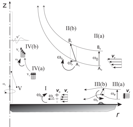
Figure 1: Schematic of vorticity evolution in intensive vortical flows.

While interactions between velocity and vorticity are commonly a destabilising factor in fluid flows, the axisymmetric vortical flows considered here have a certain stabilising mechanism linked to evolution of vorticity. If a disturbance is introduced into these flows, the generated tangential vorticity $\omega_{\theta}$ tends to compensate for this disturbance and preserve the overall structure of the flow. This effect is illustrated in figure 1 where case III shows the flow over an axisymmetric small disturbance and vorticity $\omega_{\theta}$ is generated to compensate for the disturbance and preserve the independence of $\gamma$ from $z$ at the leading order. More detailed explanations of the stabilising evolution of vorticity and a full asymptotic solution for this problem are given in Klimenko (2001c). A similar mechanism, which acts to compensate for deviations from the power-law (58), is analysed in this subsection.

Figure 1 also illustrates the direction of vorticity $\omega_{\theta}$ which tends to be generated in the vortical flows of this geometry. There are several effects, both inviscid and viscous, that are responsible for the presence of negative $\omega_{r}$ generating $\omega_{\theta}$ according to equation (8). The first effect is, essentially, the Ekman effect. If  $v_{\theta}=0$ at the lower boundary this corresponds to negative vorticity $\omega_{r}$ that generates vorticity $\omega_{\theta}$ in the direction shown in figure 1 (case I). Another effect appears due to the existence of vertical shear in a typical profile of $v_{r}$ (case II in figure 1). This shear may appear due to no-slip conditions at the lower boundary or due to inviscid effects in a bathtub flow (see Klimenko, 2001a for details). Consistency between the strong vortex and the boundary layer induced by the no-slip conditions acts as a factor constraining the flow (Turner, 1966).

Assuming that the vorticity vector is frozen into the flow (as illustrated by the joint evolution of the vorticity and material vectors transforming $\overrightarrow{\text{A}_{0}\text{B}_{0}}$ into $\overrightarrow{\text{A}_{1}\text{B}_{1}}$), this shear causes the presence of negative $\omega_{r}$ at location IIb in figure 1. Faster rotation at smaller radii turns the vorticity vector away from the reader, resulting in the appearance of $\omega_{\theta}$ in the direction shown. Although the exact convective mechanisms of generating tangential vorticity $\omega_{\theta}$ may be somewhat different for different vortices, generation of $\omega_{\theta}$ acting in the direction of lowering the values of exponent $\alpha$ below $2$ and stimulating updraft (as illustrated by case IV in figure 1) is common for the intensive vortices.

Many vortical flows have a sufficiently wide range of radii to create conditions for substantial amplification of axial vorticity. Since different characteristic radii can be characterised by different characteristic values of $K$, the localised version of the vortical swirl ratio is introduced and defined in terms of local parameters by

$$K_{r}^{2}=\frac{\gamma\omega_{z}}{v_{z}^{2}}\sim\frac{\gamma}{c^{3}r^{3\alpha-4}}\sim\frac{\gamma_{0}+\gamma_{1}}{c^{3}r^{3\alpha-4}}\;.$$ (66)

Here and in the rest of this subsection, equations (50)-(56) with power-law approximation of the streamfunction $f(r)=cr^{\alpha}$ are used. The subscript ”$r$” indicates that $K_{r}$ is radius-dependent: in principle, the local vortical swirl ratio $K_{r}$ may exhibit a strong dependence on $r.$ If, for example, $\alpha=2,$ then $K_{r}\rightarrow\infty$ as $r\rightarrow 0$. According to equation (44), $\alpha=2$ corresponds to a flow with $\omega_{\theta}=0$ (i.e. with potential image on the $r$-$z$-plane), while smaller values of $\alpha<2$ imply higher values of vorticity $\omega_{\theta}$ and more rapid increase of $\omega_{\theta}$ towards the axis as $r\rightarrow 0$. The relative magnitude of vorticity $\omega_{\theta}$ generated in the vortical flow is determined by the local vortical swirl ratio $K_{r}$. The parameter $K_{r}$ cannot unrestrictedly decrease towards the axis ($r\rightarrow 0$) since small values of $K_{r}$ correspond to negligible $\omega_{\theta}$ and, consequently, to $\alpha\rightarrow 2,$ which results in $K_{r}$ increasing towards the axis according to (66). At the same time $K_{r}$ cannot unrestrictedly increase towards the axis as this would produce large quantities of $\omega_{\theta}$ that decrease the effective value of $\alpha$ up until $K_{r}$ is forced by (66) to decrease towards the axis. This mechanism compensating for changes of $\alpha$ is reflected in equation (64).

While excessively low values of $K_{r}$ render the strong swirl approximation inapplicable, excessively large values of $K_{r}$ can cause bifurcations or destabilise the flow. Theory for vortex breakdown in steady-state axisymmetric inviscid flows governed by the Long-Squire equation was introduced by Benjamin (1962) and applied to confined vortices by Escudier et al. (1982). Klimenko (2001b) found that Benjamin’s theory can be used near the axis of intensive vortical flows, where the axial component of velocity is dominant (case IV in figure 1). The Benjamin equation (which represents a perturbed version of the Long-Squire equation) has a useful analytical solution for the power-law dependence of $K_{r}$ on $r$ (see Klimenko, 2001b). This solution indicates that, if $K_{r}\rightarrow\infty$ as $r\rightarrow 0,$ then vortex breakdown is expected according to this solution.

It follows that, although $K_{r}$ can depend on $r$ according to the definition of this parameter, this dependence should be weak when the swirl is strong. Indeed, the condition $K_{r}\sim\mathop{\mathrm{c}onst}$ ensures that the tangential vorticity is neither overproduced to destabilise the flow nor underproduced to result in the contradictions mentioned above. The regime that corresponds to these conditions and compensates for possible increases or decreases of $K_{r}$ is called here the compensating regime. The mechanism of vorticity/velocity interactions associated with this regime co-balances $v_{z}^{2}$ with $\gamma\omega_{z}$ and counter-balances $\omega_{z}$ with $\gamma$ to keep $K_{r}\sim\mathop{\mathrm{c}onst}$.

The compensating regime is linked to the compensating value of the exponent $\alpha$. Consider the two circulation terms retained in (66): $r$-independent $\gamma_{0}$ and $r$-dependent $\gamma_{1},$ which is linked to $\omega_{z}$ by (53) so that $\gamma_{1}\sim r^{2-\alpha}.$ The relative magnitudes of the terms $\gamma_{0}$ and $\gamma_{1}$ in (66) combined with the condition $K_{r}\sim\mathop{\mathrm{c}onst}$  determine different expressions for the compensating value $\alpha^{\ast}$ of the exponent $\alpha$

$$\ \begin{array}[]{cc}\alpha^{\ast}=4/3,&\gamma_{0}\gg\gamma_{1}\\ \alpha^{\ast}=3/2,&\gamma_{0}\ll\gamma_{1}\end{array}$$ (67)

Practically, this means the exponent $\alpha=\alpha^{\ast}$ of the compensating regime is not a fixed value but is represented by the range of $4/3\leq\alpha^{\ast}\leq 3/2.$ If $\alpha<4/3$ over a wide range of radii, the strong swirl cannot form at the axis. If $\alpha>3/2$ persists, large $K_{r}$ near the axis would cause vortex breakdown followed by weakening of the swirl. Unsteady effects are discussed in the next subsection and in Appendix B.

The asymptotic analysis of the previous subsections requires that $\gamma_{1}/\gamma_{0}\sim\mathop{\mathrm{S}t}\ll 1$ in expansion (30) or, otherwise, expansions (30) would formally lose asymptotic precision. The condition $\gamma_{1}/\gamma_{0}\ll 1$ corresponds to $\alpha^{\ast}=4/3$ obtained in equation (58), which neglects losses of $\gamma_{0}$ and thus considers this term as dominant. Note that $\gamma_{0}\gg\gamma_{1}$ is not necessarily the case in realistic vortices due to vortex breakdowns and loss of angular momentum into the ground (which are not taken into account in the idealised considerations). Since $\gamma_{1}$ increases with increasing $r$, the outer sections of the intensification region are more likely to have a larger value of $\alpha^{\ast}$ (within the compensating range) than the inner sections.

The compensating exponent is thus extended from the value $\alpha^{\ast}=4/3$ to the range of $4/3\leq\alpha^{\ast}\leq 3/2$. The mechanism of evolution of vorticity in converging flows, which is reflected by equation (64) and explained above, acts to compensate for changes of $K_{r}$. The downstream relaxation of $c(r)$ to its constant value $c_{0}$ governed by (64) implies that $K_{r}$, which is defined by (66) and linked to the inverse third power of $c$, undergoes a similar relaxation to its radius-independent value.

3.5 Evolution of the vortex

This subsection considers some of more complex transient effects in the formation and breakdown of intensive vortices. Typically, the formation of intensive vortices starts when a converging fluid motion occurs in the presence of some background axial vorticity. One can assume that the vorticity is initially distributed as in solid body rotation, $\omega_{z}=\omega_{0}=\mathop{\mathrm{c}onst}$. The initial value of the vortical swirl ratio $K_{r}$ is small and rotation in the flow is not intense. The focus of the present consideration is a near-axis region $r\leq r_{2}$ where the stream function can be represented by $\psi=c_{0}r^{\alpha}z$. Since, initially, $K_{r}$ is uniformly small in this region, the flow image on the $z$-$r$-plane is potential and $\alpha=2$. In this case $v_{z}=v_{0}=\mathop{\mathrm{c}onst}$ at a given height $z=z_{0}$. This region is primarily responsible for formation of the vortex. The other limiting case of $\alpha=0$ corresponds to two-dimensional flow called a vortical sink. This flow may be relevant to more peripheral regions of the vortex where the value of $K_{r}$ does not change significantly even without the presence of the compensating mechanism. The inviscid solutions for evolution of vorticity and circulation are presented in Appendix B.

In the case of $\alpha=2,$ the value of $K_{r}$ is specified by the following expression

$$K_{r}^{2}=\frac{\gamma\omega_{z}}{v_{z}^{2}}=\exp(4\tau)\frac{\omega_{0}^{2}}{2v_{0}^{2}}r^{2},$$ (68)

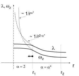
Figure 2: Schematic of development of the axial vorticity and horizontal convergence during formation of an intensive vortex; current (——) and quasi-steady (– – –) distributions are shown.

where $\tau$ is a time-like variable defined in Appendix B. The parameter $K_{r}$ rapidly increases with time and one can note that the quasi-steady distribution of axial vorticity $\omega_{z}\sim 1/r^{\alpha}$ is never achieved as long as $\alpha$ remains 2. The growth of $K_{r}$ can not continue indefinitely and at a certain moment $K_{r}\sim 1$ is achieved at the outer rim of the region under consideration where, say, $r=r_{1}=r_{2}$. The value $r_{2}$ representing the radius of the domain is kept constant, while the radius $r_{1}(t)$ where $K_{r}\sim 1$ continues to decrease according to equation (68). The nature of the flow in the ring $r_{1}<r<r_{2}$ changes so $\alpha$ decreases and becomes close to $\alpha^{\ast}$ since large values of $K_{r}$ are attained there. Since $\alpha<2$ within the ring, the convergence of the flow increases towards the axis. The equations presented in Appendix B show that the axial vorticity does approach the quasi-steady distribution $\omega_{z}\sim 1/r^{\alpha}$ when $\alpha<2$. In the region $r<r_{1}(t)$ the value of $K_{r}$ is small and insufficient to change the nature of the flow, hence $\alpha=2$ remains there. Figure 2 gives a schematic illustration of the formation of an intensive vortex. Both the stretch $\lambda$ and axial vorticity $\omega_{z}$ evolve from initial constant values to quasi-steady exponents of the compensating regime (see also Appendix B). Formation of the vortex is completed when $r_{1}$ approaches the axis and becomes small. This formation is characterised by $\alpha$ falling from 2 to $\alpha^{\ast}$ in $\psi\sim r^{\alpha}z$, while the axial vorticity, which is initially constant, increases its radial slope to converge to $\omega_{z}\sim 1/r^{\alpha},$ where $\alpha$ reaching $4/3$ is needed for a strong swirl to appear near the axis.

During formation of the vortex, the flow undergoes a significant change. Initially, when $K_{r}\ll 1$, the vorticity is present in the flow as a passive quantity that is transported by the flow but does not significantly affect the velocity field. At this stage the flow image on the $r$-$z$ plane can be treated as potential since the vorticity level is low. A potential flow immediately (with the speed of sound) reacts to any disturbance at the boundaries of the domain under consideration and specifying the velocity field at some imaginary boundaries of the flow uniquely determines the flow within the region. The convergence point (which is selected as the origin of coordinates $r=0$ in the axisymmetric model) is also fully determined by the conditions on the imaginary boundary somewhere in the peripheral region of the flow. In practice, this means that the convergence point would move promptly and randomly if random disturbances are present at the periphery of the flow, or the flow may even have several convergence points at a given moment.

When the vortical swirl ratio $K_{r}$ becomes sufficiently large, a noticeable amount of tangential vorticity $\omega_{\theta}$ is generated. The structure of the flow changes, producing higher convergence near the axis and compensating further increases in vorticity to keep $K_{r}$ constant. In this case, as discussed previously, vorticity exhibits some stabilising effect on the flow. When the vortex is formed, the stabilising effect of vorticity propagates towards the axis as $r_{1}$ decreases. The tangential vorticity $\omega_{\theta}$ stimulates updraft near the flow axis and vorticity evolves in time but does not respond immediately to fluctuations at the boundaries of the region under consideration. This makes the position of the centre of convergence, which is also the centre of the vortical motion in our model, more stable. In this vortex, rotation is intense and the vortex is now fully perceived as an intensive vortex.

Qualitative evolution of vorticity during the formation of a strong vortex is shown in figure 2. Initially, the value of $\gamma_{0}$ defined in (53) can be negative but, as the vortex forms, both $\omega_{z}$ and $\gamma_{0}$ increase. Without losses, the value of $\gamma_{0}$ continues to grow slowly but unrestrictedly; although, practically, any substantially positive value of $\gamma_{0}$ would induce high velocities near the axis $v_{\theta}\sim r^{-1},$ amplifying the losses of angular momentum in the vicinity of the vortex core. A typical intensive vortex remains stable and seems to be nearly stationary. The state of the vortex flow, however, is determined by two major effects that control the relative magnitude of $\gamma_{0}$ in (53): the increase of angular momentum due to inflow from peripheral regions and the loss of angular momentum into the physical boundaries of the flow. If the influx of momentum exceeds its losses, $\gamma_{0}$ continues to grow. While changes in the balance of influx and losses may also disturb the vorticity profile, the equilibrium state for this profile is specified by the exponents of the compensating regime. As previously discussed, relatively large values of $\gamma_{0}$ are sustainable when $\alpha^{\ast}=4/3$.

A persistent growth in $\gamma_{0}$ can increase $K_{r}$ to the level when the flow bifurcates (as discussed in the previous subsection). The analysis of the viscous core in Appendix A indicates that the singularity of $\alpha=\alpha^{\ast}$ in $\psi\sim r^{\alpha}z$ disappears near the axis and the value of $K_{r}$ is higher in the core than in the surrounding inviscid flow; hence the bifurcations are likely to appear first in or near the core (schematically shown as region V in figure 1). This effect, which causes reversal of the flow at the axis (i.e. from updraft to downdraft), is known as vortex breakdown (see, for example, Escudier et al., 1982; Lewellen, 1993; Church and Snow, 1993; Lee and Wurman, 2005). Axial downdrafts are common during late stages of development of very intensive vortices (Church and Snow, 1993; Emanuel, 2003). Vortex breakdowns affect the structures of the cores of tornadoes and the eyes of hurricanes by terminating the centripetal flow near the axis and thus reducing the relative value of $\gamma_{0}$. The balanced value of $\alpha^{\ast}$ that corresponds to negligible $\gamma_{0}$ is $3/2.$

The vorticity equations allow for an alternative scheme of vortex formation. Let us assume that the initial $K_{r}$ is small and that $\omega_{z}$ is initially distributed in a quasi-steady manner $\omega_{z}\sim 1/r^{\alpha}$. Since $K_{r}$ is small, $\alpha=2.$ Under quasi-steady conditions, the vortical swirl ratio is given by equation (66) $K_{r}\sim\gamma/r^{2}$. As $\gamma$ increases due to additional angular momentum brought from peripheral regions, $K_{r}$ becomes large first near the axis and the radius $r_{1}(t)$ of $K_{r}\sim 1$ then moves sideways. The compensating regime appears first near the axis $\alpha=\alpha^{\ast}$ at $r<r_{1}$ and propagates sideways (where $\alpha=2$ at $r>r_{1}$). This scheme was visualised by Klimenko (2001a) as a series of quasi-steady pictures of calculated streamlines. This scheme, although possible, raises a question: why is the quasi-steady solution reached in the first place under conditions when $\alpha=2$ while, according Appendix B, $\omega_{z}$ approaches the quasi-steady solution only when $\alpha<2$? Note that $\psi\sim r^{\alpha}z$ is only the leading term in representation of the stream function and the solution $\omega_{z}=\omega_{0}\exp(2\tau)$ may, in principle, be altered by the other terms.

The formed intensive vortex is quite stable but does not persist forever. If vorticity with a dominant direction is initially present in the tub, the bathtub vortex is likely to persist until the tub is emptied, but intensive vortices in the atmosphere can weaken and disappear for various reasons. The influx of axial vorticity can become exhausted at a certain moment (due to weakening of the recirculating motion or insufficient axial vorticity level in the peripheral regions) but this does not mean that the vortex disappears immediately. A significant amount of axial vorticity can be concentrated in the viscous core (see Appendix A) and will maintain visible rotation even if $\omega_{z}=0$ in the surrounding flow. This case corresponds to $\alpha=2$ in $\psi\sim r^{\alpha}z$ since $K_{r}=0$ outside the core. At this stage, the vortex can be characterised by the conventional stationary axisymmetric solution of Lewellen (1962). Practically, the vortex would continue to lose angular momentum to the physical boundaries of the flow until it fully disappears.

4 Atmospheric vortices

Examples of intensive vortices of different scales are considered in this section. The smallest vortex can be observed in a bathtub flow while the largest are represented by atmospheric vortices – dustdevils, firewhirls, tornadoes, mesocyclones and cyclones. For bathtub flows, the compensating exponents have been observed in computations (Klimenko, 2001a; Rojas, 2002) and experiments (Klimenko, 2007; see also Shiraishi and Sato, 1994). The atmospheric vortices are quite different from the bathtub vortex and from each other. These differences stem from differences in scales and the physical mechanisms that are responsible for the formation of these vortices. There are, however, features that are common: the vortices can usually be characterised by certain inner (core) scales and are embedded into outer flows. As discussed in the previous sections, the present work does not seek a complete description of these vortices; rather it neglects less significant details (for example, rain bands of a hurricane) and focuses on the main features of the average flow in the intensification region, which, from the asymptotic perspective, is an intermediate region between the inner and outer scales of the vortex. This region is characterised by the presence of the axial vorticity and its continuing amplification. Due to the reduced number of parameters needed to characterise the intensification region, vortices of different scales may exhibit a greater degree of similarity within this region. Among atmospheric vortices, cyclones, tornadoes and, on some occasions, firewhirls are characterised by an extended range of scales, greater stability and resistance to atmospheric fluctuations (due to the enormous scales of tropical cyclones, the high wind speeds achieved in tornadic flows, and the extreme energies released by fires). This, of course does, not mean that these vortices are completely regular – the flow patterns in cyclones and especially in tornadoes reflect irregularities of surrounding atmospheric motions and display significant variation of flow parameters.

Tangential winds, which possess a significant inertia and are the strongest in atmospheric vortices, are commonly reported and discussed in publications. Tangential winds tend to be least affected by the surface boundary layer and outer disturbances always present in the atmosphere. Equations (60) indicate that the tangential velocity and axial vorticity of intensive vortices can be approximated by the following power laws

$$v_{\theta}=\frac{\gamma}{r}=\frac{\gamma_{0}}{r}+\frac{c_{1}}{(2-\alpha)r^{\beta}}+...,\;\;\omega_{z}=\frac{1}{r}\frac{\partial\gamma}{\partial r}=\frac{c_{1}}{r^{\alpha}}+...,\;\;\beta=\alpha-1$$ (69)

and checked against experimental measurements. Equations (69) have a two-term expression for $v_{\theta},$ while the corresponding approximation for $\omega_{z}$ involves only one term. In many realistic vortices, $\gamma_{0}$ is small compared to the second term and either can be neglected or can not be reliably determined from data available for a limited range of radii. When $\gamma_{0}$  is substantially positive, attempting to fit the tangential velocity data by a single term $v_{\theta}\sim 1/r^{\beta}$ would result in overestimating $\beta$. Hence, comparison of the theory and measurements based on vorticity is more direct but, if significant noise is present in the data, numerical differentiation of velocity profile can produce high levels of scattering.

4.1 Firewhirls

Firewhirls are fires that are characterised by the presence of a strong rotation in the flow resulting in elongated and more intense flames (Williams, 1982). Once firewhirls appear in a fire, they greatly intensify burning and are very difficult to extinguish. The scales of firewhirls are generally comparable to those of tornadoes, which are discussed in the following subsection. In firewhirls, however, the centripetal flow is stimulated by a large heat release and buoyant uplifting, which should prevent the vortex breakdowns and axial downdrafts typical in other intensive atmospheric vortices. Firewhirls observed on inclined surfaces are most interesting as they can deviate from the vertical direction and become perpendicular to the inclined ground surface. As discussed by Chuah et al. (2011), this indicates dominance of vortical effects over buoyant uplifting and links firewhirls with other intensive vortical flows, although the presence of density variations and buoyancy remains essential in firewhirls.

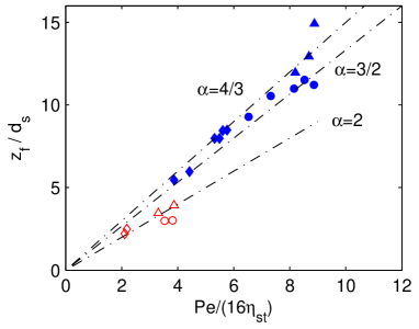
Figure 3: Firewhirl length $z_{f}$ versus Pe number. Experiments by Chuah et al. (2011): open symbols – no rotation; solid symbols – with rotation. Dash-dotted lines – theory by Klimenko and Williams (2013) corresponding to $\alpha=4/3$, 3/2 and 2; $d_{s}$ is the diameter of the fuel source; $\eta_{st}$ is the stoichiometric value of the mixture fraction.

Klimenko and Williams (2013) have recently extended the analysis of Kuwana et al. (2011) and introduced a theory, that uses velocity approximations based on the compensating regimes and determines the normalised flame length in terms of the Peclet number and the effective value of the exponent $\alpha$. While Klimenko and Williams (2013) take into account the presence of the viscous/diffusive core, figure 3 presents a simplified treatment linked to the power laws with characteristic values of $\alpha$ used in the rest of the present work: 2, 3/2 and 4/3. The value $\alpha=2$ is associated with flows that have a potential image on the $z$-$r$-plane, while the compensating range of $4/3\leq\alpha\leq 3/2$ is applicable to the case when rotation in the flow is strong. While buoyancy prevents vortex breakdowns and thus favours the exponent of $4/3$ over $3/2,$ the presence of diffusivity acts in the direction of increasing the effective value of the exponent $\alpha$. The experimental points of Chuah et al. (2011) shown in figure 3 are in a good agreement with the theoretical predictions.

4.2 Supercell tornadoes

Tornadoes are more affected by atmospheric disturbances than tropical cyclones and, typically, demonstrate noticeable fluctuations of the axial vorticity at different elevation levels, while in a strong swirl the vorticity $\omega_{z}$ is independent of $z$ to the leading order of approximation. In tornadoes, the region of interest has a characteristic AGL (above ground level) of several hundred meters. For the purpose of comparison, the largest and most stable tornadoes need to be selected as they are least affected by atmospheric fluctuations, have an axisymmetric (or near-axisymmetric) structure with uniform distribution of vorticity at different altitudes and the largest possible range of radii of the intensification region. As discussed previously, the stages when the axial vorticity is exhausted in surrounding flow are best described by conventional Burgers vortices and are different from the intensification stage considered in the present work. According to Fujita (1981), the strongest tornadoes reaching F4 grades on the Fujita scale represent less than 3% percent of all occurrences of tornadoes while F5 tornadoes are rare. The strongest and most stable tornadoes with intense rotation are usually embedded into the core region of a mesocyclone as a part of supercell thunderstorms.

The exponent $\beta=\alpha-1$ in $v_{\theta}\sim 1/r^{\beta}$ has been occasionally reported for large tornadoes. Wurman and Gill (2000) presented high resolution measurements of F4 tornado formed in a supercell storm near Dimmitt, Texas in 1995 and reported a tangential velocity profile approximated within the range of $100\mathop{\mathrm{m}}<r<1$km by a power law with $\beta=0.6\pm 0.1.$ Lee and Wurman (2005) presented measurements for a large F4 tornado that hit a small town of Mulhall in Oklahoma in 1999. The tornado was unusual: it had a very large core with the radius of maximal winds $r_{m}$ (RMW) nearly reaching 1km scale and multiple vortices orbiting the common core (Wurman, 2002). The overall slope of axisymmetric profiles of tangential velocity within the range of 1km to 3km is reported as having $0.6\leq\beta\leq 0.7,$ although $\beta$ has significant variations within this range of radii. The slope of the profiles within the range of $1<r/r_{m}<1.5$ is around $\beta=0.5$ or lower, although increases in $\beta$ outside the radius of $1.5r_{m}$ (or $2r_{m}$ for some of the profiles) indicate that axial vorticity was small or negative in this region – this corresponds to $\beta\approx 1$. Wurman (2002) later reported $0.5\leq\beta\leq 0.6$ for this tornado.

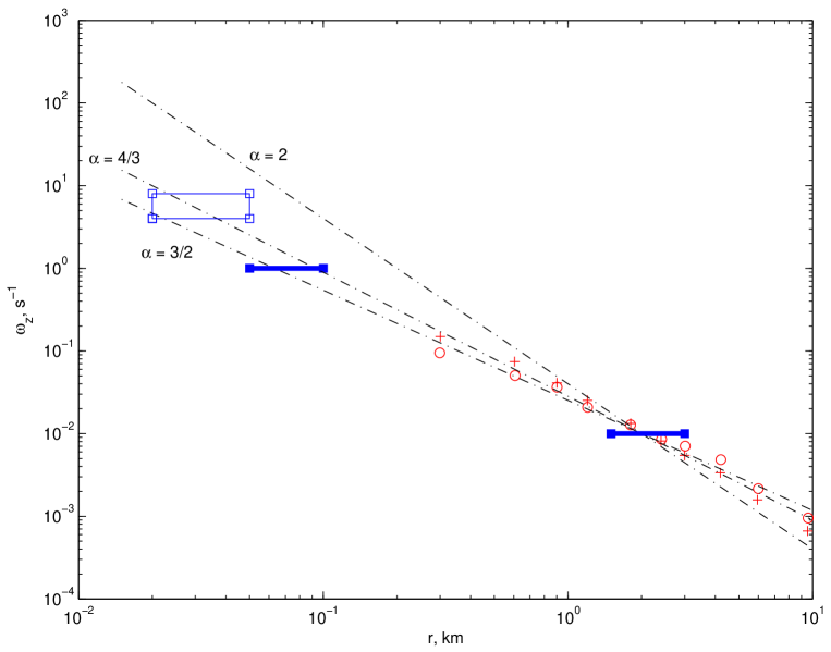
Figure 4: The range of radii characterising the inner and outer scales of a typical mesocyclone tornado and the corresponding typical levels of axial vorticity at these scales. The values of typical parameters are taken from Brooks et al. (1993), Dowell and Bluestein (2002), Bluestein and Golden (1993) and other publications ($\blacksquare$—$\blacksquare$). Maximal vorticity ever measured in tornadic flows as reported by Wurman (2002) ($\Box$—$\Box$). Symbols: the scaling of maximal mesocyclonic vorticity versus grid spacing as reported by Cai (2005) for storms at Garden City ($+$) and Hays (o). The dash-dotted lines demonstrate the slope of $\omega_{z}\sim 1/r^{\alpha}$ for $\alpha=2,$ $3/2,$ $4/3$.

As mentioned previously, the vorticity-based comparison of theory and measurements is more direct. The consistency of the power laws of the compensating regime is now examined in comparison with the conventional estimations of vorticity levels in tornadic flows. According to reviews of atmospheric measurements by Brooks et al. (1993), Bluestein and Golden (1993), and Dowell and Bluestein (2002), a typical supercell tornado amplifies its axial vorticity from $\sim 0.01$s^-1 in the outer region with a span of $3$-$7$km to a level of $\sim 1$s^-1 in the core of the tornado with a scale of $\sim 100$m. Figure 4 illustrates the comparison of these parameters with the power laws $\omega_{z}\sim 1/r^{\alpha}.$ The thick lines show the radius of $1.5$-$3.5$km corresponding to the scale  $3$-$7$km for the surrounding vorticity of $\omega_{z}=0.01$s^-1 and the radius of $50$-$100$m corresponding to the scale of $100$-$200$m for the vorticity of $\omega_{z}=1$s^-1 in the tornadic core.  The box indicates Wurman’s (2002) estimate for the highest vorticity ever measured in tornadoes, which has been detected in multiple vortices of the Mulhall tornado. This vorticity reached 4–8s^-1 and within scales of 40–100m. The compensating exponents $\alpha=4/3$ and $\alpha=3/2$ are reasonably consistent with the commonly accepted characteristics of supercell tornadoes.

Cai (2005) reported fractal scaling of vortical characteristics of a mesocyclone, which are expressed as maximal vorticity $\left(\omega_{z}\right)_{\text{max}}$ measured on a given grid versus grid spacing $r_{g}$. The characteristic axial vorticity $\omega_{z}$ at the distance $r_{g}$ from the flow convergence centre can serve as an estimate for $\left(\omega_{z}\right)_{\text{max}}$. Several mesocyclones have been analysed and it was found that, as expected for fractals, the scaling can be accurately approximated by the power law $\left(\omega_{z}\right)_{\text{max}}\sim 1/r_{g}^{\alpha}$. Cai (2005) found that during intensification of the Garden City tornadic mesocyclone $\alpha$ increased from 1.31 to 1.59, while for the non-tornadic Hays mesocyclone the value $\alpha$ ranged only from 1.23 to 1.32 not reaching 4/3 — the lower boundary of the compensating exponent predicted by the presented theory. The scaling profiles for the highest $\alpha$ reported by Cai (2005) are shown in figure 4. It seems that Cai’s fractal method can recover regular exponents for radii reaching 10km, where the mesocyclonic flow becomes quite irregular.

Several tornadoes that appeared in the 1995 McLean (Texas) storm were measured by a Doppler radar (Dowell and Bluestein, 2002) and were also surveyed and photographed from the ground (Wakimoto et al. 2003). Among these tornadoes, tornado 4 was the strongest, largest and most stable tornado, reaching a rating of F4-F5 on the Fujita scale. Unlike the other tornadoes in this storm, the axial vorticity in tornado 4 was fairly uniform up to AGL of more than 4 km, it had a regular, nearly axisymmetric shape, and it persisted for more than an hour.  The ground damage survey by Wakimoto et al. (2003) indicates that the radius of maximal winds and the corresponding damage (F3 at 23:38 UTC, Coordinated Universal Time) did not exceed $150$m. The axial vorticity has been determined a) from the contour plot by calculating the average radius of each vorticity contour line and b) from the reported circulation $\gamma(r)$ under assumptions of an axisymmetric flow. The results are shown in figure 5 for the tornadic range of radii ($r\leq 4$km) and are reasonably consistent. The error bars show the standard deviations in evaluating average radii — large deviations are indicative of a non-axisymmetric flow. The increasing difference between the curves at $r>1$km is explained by the difficulty of evaluating $\omega_{z}(r)$ from $\gamma(r)$ due to an increasingly non-axisymmetric structure of the flow at mesocylonic scales. Note that the exponents of the compensating regime $4/3\leq\alpha\leq 3/2$ produce a reasonable match to the measured vorticity levels.

Dowell and Bluestein (2002) also reported the convergence rates during formation of tornado 4. According to the analysis of the vortex evolution in Section 3.5, a constant convergence rate $\lambda$ that corresponds to initially weak swirl with $\alpha=2$ in (59) is gradually replaced by the convergence rate increasing towards the axis according to $\lambda\sim r^{\alpha-2}$ and the value $\alpha$ belonging to the compensating range. As illustrated in figure 2, this replacement occurs through extension of the compensating regime towards the axis. The convergence profiles reported by Dowell and Bluestein (2002) are consistent with the scheme illustrated in figure 2.

4.3 Tropical cyclones

Tropical cyclones are the largest and most stable vortices observed in the Earth’s atmosphere. The core region of the cyclone consists of the eye surrounded by the eye wall and, in most cases, has a characteristic radius of around 20—40km. This region has a noticeably higher temperature and is strongly affected by buoyancy, while the temperature increments in the surrounding flow are much smaller. The maximal wind speeds are achieved within the outer rim of the core. The intensification region, which is located just outside the core region and above the surface boundary layer, also involves reasonably strong tangential winds. This region is characterised by the presence of some updraft flow of air (which is, of course, weaker than the updraft in the eye wall). The radial winds (and, to lesser extent, the tangential winds) are affected by the Ekman effect near the ground or sea surface; hence measurements outside the immediate surface boundary layer should be preferred in the context of our analysis. The intensification region is limited by its outer radius, which can stretch beyond 100km. The region located outside the intensification region is also subject to strong influence from the cyclone. The radius of this region, which is called here ”peripheral”, can extend to 500 km and, possibly, beyond. The peripheral region can be can be seen as a two-dimensional vortical sink without any significant updraft. The more remote sections of this region are affected by fluctuations of synoptic weather patterns.

Approximating the tangential velocity profile in the form of the power law $v_{\theta}\sim 1/r^{\beta}$ is conventional in cyclone-related literature. This power law implicitly assumes that $\gamma_{0}\approx 0$ in (69) and this may be adequate for many tropical cyclones. Although $\beta$ may experience some variations, the estimates $\beta=-1$ for the core region, $\beta=0.5$ for the intensification region and $\beta=1$ for the peripheral region are common in the literature (Gray, 1973; Emanuel, 2003). Although $\beta=0.5$ is considered to be the best average approximation in the intensification region (Gray, 1973; Emanuel, 2003), some estimates of $\beta$ can deviate from this value. For example, one of the early works by Hughes (1952) nominated $\beta=0.62$ as the best fit to data obtained from a number of reconnaissance flights into cyclones (these flights began in 1943 and represent the most important source of information about hurricanes) and he noted that this exponent is reasonably close to the more conventional value of $\beta=0.5$. Riehl (1963) observed evolution of unusual tangential wind profiles in hurricanes Carrie (1957) and Cleo (1958) relaxing towards profiles with $\beta\approx 0.5$.

Explaining the value of $\beta=0.5$ in the intensification region is not trivial. Riehl (1963) demonstrated that $\beta=0.5$ produces a good fit for $v_{\theta}\sim 1/r^{\beta}$ in six different hurricanes. He noted that assuming both the moment of the tangential component of the surface stress $r\sigma_{\theta}$ and the drag coefficient $C_{D}$ to be independent of $r$ is sufficient (but not necessary) for $\beta$ to be $0.5.$ Although Pearce (1993) put forward arguments supporting this assumption, the independence of $C_{D}$ from $r$ is generally not supported by the measurements. The data reported by Hawkins and Rubsam (1968) and by Palmen and Riehl (1957) indicate, however, that $C_{D}\sim 1/r^{\zeta}$ with $\zeta$ ranging between 0.4 and 0.7 while Palmen and Riehl (1957) determined that, on average, $r\sigma_{\theta}\sim 1/r^{0.6}$. The approach of the present work indicates that, while losses of angular momentum are important in intensive vortices, the flow adjusts itself to compensate for disturbances and relax towards the exponents of the compensating regime. In his thermodynamic theory of steady tropical cyclones, Emanuel (1986) demonstrated that $\beta\approx 0.5$ just outside RMW is consistent with typical temperatures on the sea surface and in tropopause. Here, one can note that $\alpha=\beta+1=1.5$ is the same as the value $\alpha^{\ast}=3/2$ suggested in Section 3 for the compensating regime.

Hawkins & Rubsam (1968) and Hawkins & Imbembo (1973) reported axial vorticity distributions and other characteristics for two hurricanes, Hilda (1964) and Inez (1966). These distributions do not show any significant dependence on $z$ at lower altitudes, although the axial vorticity profile of Hilda had an irregularity at the altitudes above two kilometers, while $\omega_{z}$ in Inez remained regular up to the altitudes of four kilometers. Vorticity distributions in these and other hurricanes tend to be reasonably consistent with the strong swirl approximation and the exponents of the compensating regime.

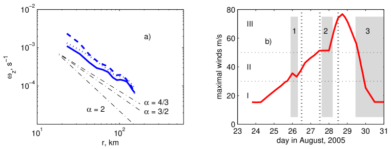
Figure 6: Hurricane Katrina, 2005. a) Axial vorticity $\omega_{z}$ versus radius $r$ measured at 12:00 26 August UTC (——); at 12:00 27 August UTC (……); at 12:00 28 August UTC (– – – –). The thin dash-dotted lines show the slope of $\omega_{z}\sim 1/r^{\alpha}$ for $\alpha=2,$ $3/2,$ $4/3$. b) Maximal winds versus versus UTC dates. The ranges for I – prehurricanes, II – minimal hurricanes and III – major hurricanes are shown (see table 1 for the definitions). The vertical dashed lines correspond to the three time moments listed above. The gray areas indicate events disturbing the state of the hurricane: 1 – the first landfall over southern Florida, 2 – eye replacement cycle, 3 – the second landfall. The data and information are taken from Knabb et al. (2005) and Powell et al. (2010). The axial vorticity is evaluated from the data set provided by Hurricane Research Division of the US National Oceanic and Atmospheric Administration (HRD-AOML-NOAA).

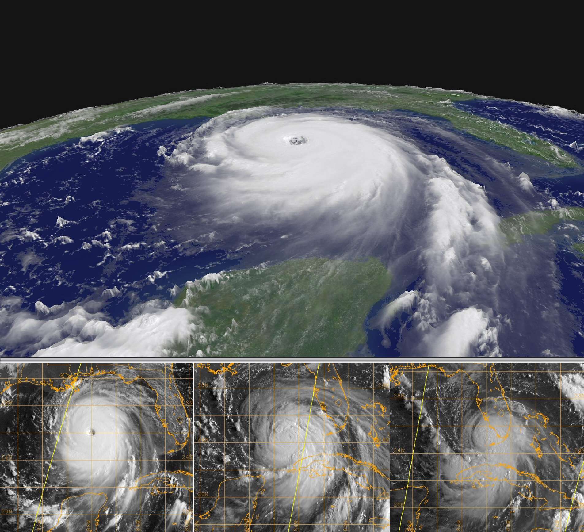
Figure 7: Satellite photographs of hurricane Katrina. Top: taken at 15:45 UTC on 28 August, 2005, when the hurricane was about to reach its maximal strength (courtesy of the NASA Goddard Space Flight Center). Bottom, from right to left: images taken on 26, 27 and 28 August at approximately the same times (i.e. 12:00 UTC) as for the data presented in figure 6a (courtesy of the US Naval Research Laboratory)

Katrina (2005) is one of the strongest hurricanes on record to hit the American continent. After passing over the southern tip of Florida (zone 1 in figure 6b), hurricane Katrina quickly regained its strength. On 27 August, Katrina reached the warm waters of the Loop Current of Mexican Gulf (Powell et al., 2010) and became a major hurricane (see table 1) but its further strengthening, was delayed due to adjustments that are likely to have been caused by the eyewall replacement cycle (Knabb et al., 2005, Houze et al., 2007). After completion of the cycle (shown as zone 2 in figure 6b), Katrina intensified at an extremely high rate, reaching category 5 on 28 August. The inclined satellite photo in figure 7 (top), taken when the hurricane was approaching its maximal strength, shows the large scale of the hurricane and a very distinct eye that forms a depression reaching a diameter exceeding 50km. This clearly visible eye is indicative of axial downdrafts and is typical of major hurricanes, although it seems that the formation of a prominent eye in Katrina was delayed by the eyewall replacement cycle until the early morning of 28 August (although the eye can be detected in infrared satellite images taken on 27 August — see Knabb et al., 2005). Katrina started to reduce its strength towards the end of 28 August, and on 29 August it made its second landfall on the Louisiana coast causing flood and devastation (shown as zone 3 in figure 6b). In the following days, Katrina quickly lost its might but, as a tropical depression, reached as far as the states near the Great Lakes and caused rains in Canada. The axial vorticity profiles are evaluated from the hurricane wind speeds and shown at 12:00 UTC on 26, 27 and 28 August, when Katrina was only a minimal hurricane, just reached the status of a major hurricane and was a major category 5 hurricane close to its peak state. The three bottom images in figure 7 illustrate the state of the hurricane at the time of the measurements. Only last of the curves (i.e. measured on 28 August) presented in figure 6a corresponds to the vortex with a large visible eye present. The profiles are generally consistent with the compensating exponents. The slope of the vorticity curves tends to increase when the hurricane becomes stronger.

Mallen et al. (2005) presented a comprehensive analysis of axisymmetric tangential velocity and axial vorticity distribution in tropical storms involving 251 different cases. The results are summarised in table 1. The scaling exponents were determined in the region between $1\leq r/r_{m}\leq$ $3$ where $r_{m}$ denotes RMW. The exponents reported for different storms indicate a significant scattering with $\alpha$ ranging from 1.05 to 1.7. The best approximation for the exponent ($\alpha=1.37$) was determined as the average over all storms. Mallen et al. (2005) also found that the value of the exponent correlates with the strength of the storms and divided all storms into three classes: prehurricanes, minimal hurricanes and major hurricanes. The average value of $\alpha$ for each of the classes were determined to be 1.31, 1.35 and 1.48. The higher values of $\alpha$ correspond to stronger storms. These profiles also have differences at $r=r_{m}$ where the slope of these profiles is much steeper than that predicted by $\omega_{z}\sim 1/r^{\alpha}$ due to the dominance of vorticity $\gamma_{0}$ accumulated within the core. As expected from the present analysis, the average vorticity profiles reported by Mallen et al. (2005) for pre-hurricanes and minimal hurricanes are flatter at $r>r_{m}$ but are nevertheless steeper at $r=r_{m}$ indicating a stronger influence of $\gamma_{0}$ on the flow just outside RMW. The major hurricanes, which belong to category three and above, usually have a clearly visible eye with a cloud clearance created by downdrafts. As discussed in Section 3.5, this corresponds to reduced influence of the core and to a compensating exponent of 3/2. Note that the range of $\alpha=$ 1.31, 1.35 and 1.48 is very close to the range of $4/3\leq\alpha\leq 3/2$ predicted by the present analysis of the compensating regime.

Table 1: Comparison of average values of the exponent $\alpha$ determined by Mallen et. al. (2005) for different hurricane classes with theoretical predictions; $n$ is the number of cases analysed; $\Delta\alpha=\alpha-\left<\alpha\right>$ is deviation of $\alpha$ from its average; $v_{m}=v_{\theta}\left(r_{m}\right)$ is the speed of maximal winds; the averages in the last line are weighted by $n$. (Note that the hurricanes of category 1 on the Saffir- Simpson scale have the maximal winds of at least 33m/s, which is very close to the 30m/s threshold for the minimal hurricanes.)

	$v_{m}$	category	$n$	measurements		theory
				$\left<\Delta\alpha^{2}\right>^{\frac{1}{2}}$	$\left<\alpha\right>$	$\alpha^{*}$
pre-hurricane	$<$30m/s	tropical storm	73	0.12	1.31	$4/3\approx 1.33$
		or depression
minimal hurricane	30-50m/s	1, 2	106	0.14	1.35	$4/3\approx 1.33$
major hurrricane	$>$50m/s	3, 4, 5	72	0.11	1.48	$3/2=1.50$
average	all	all	251	0.14	1.37	1.38

5 Conclusions

The present work develops a theory of intensive vortices that are distinguished by a fluid flow from peripheral to central regions and a significant amplification of rotational motion near the centre of the flow. The theory is generic and based on the strong swirl asymptotic appoximation, considered from the perspective of vorticity equations. Hurricanes, tornadoes and firewhirls, which are also examined in the present work, are well-known examples of intensive vortices. Conventional axisymmetric vortical schemes that imply a potential flow image on the axial-radial plane (such as the Burgers vortex) do not represent a good model for an intensive vortex with significant ambient vorticity and strong swirl. In terms of the power law $\psi\sim r^{\alpha}z$, flows with a potential $r$-$z$-image correspond to $\alpha=2,$ while the present theory of intensive vortices suggests that the exponent $\alpha$ should reach its compensating values $\alpha^{\ast}$ lying in the range of $4/3\leq\alpha^{\ast}\leq 3/2$. This exponent is expected to be valid outside the core extending outward to the intensification region, where updrafts amplifying the axial vorticity are significant. The compensating values of the exponent are determined by consistency of velocity/vorticity interactions that, in axisymmetric conditions considered here are, controlled by the vortical swirl ratio $K$. This parameter $K=(S/\mathop{\mathrm{R}o})^{1/2}$ represents the geometric mean of two conventional parameters — the swirl ratio and the inverse Rossby number.

While intensive vortices tend to evolve slowly, they are still inherently non-stationary and evolutionary aspects of these vortices need to be considered. Formation of the vortex involves appearance of strong swirl condition at a distance from the centre followed by centripetal propagation of these conditions. In the regions where the swirl becomes strong, the exponent $\alpha$ relaxes to its compensating range. This scheme is different from the centrifugal propagation of these conditions considered by Klimenko (2001a). Two aspects of the influence of viscosity on the core of the vortex are of interest. First, the value of $K$ in the viscous core is higher than in the surrounding flow, which creates conditions for the vortex breakdown in the core. Second, viscosity is shown to remove the singularity of the compensating exponents near the axis.

Interactions of velocity and vorticity are generally known to have a destabilising effect in most of the fluid flows. In intensive vortices, however, these interactions enact a stabilising mechanism that compensates for possible variations of the vortical swirl ratio and, as the fluid flows towards the axis, relaxes the exponents to their compensating range $4/3\leq\alpha^{\ast}\leq 3/2$. Existence of this stabilising mechanism explains the persistent character of the intensive vortices. The compensating exponents can be seen as equilibrium values — the actual exponents measured in the specific vortices may deviate from but tend to relax to these equilibrium values. In the atmosphere, intensive vortices are continuously disturbed by changes in surrounding atmospheric and surface boundary conditions. The measurements presented here indicate a reasonable but not absolute agreement with the theory when specific cases are analysed. However, when the averages are evaluated over a large set of experiments (251 hurricanes analysed by Mallen et al. 2005) and the disturbances and variations of conditions are effectively removed, the match between theoretical predictions and experiments becomes very accurate.

Appendix A Viscous core in the strong swirl approximation

This section proves that the singularity of the compensating regime is removed by viscosity near the axis, and finds the corresponding consistent asymptotic at $r\rightarrow 0.$ In the viscous core, the influence of viscosity is significant and the characteristic radius $r_{\ast}=\nu/(Lv_{\ast})$ is determined by $\mathop{\mathrm{R}e}=1$.  Since $\mathop{\mathrm{R}e}_{z}\equiv z_{\ast}v_{\ast}/\nu=\mathop{\mathrm{R}e}/L\gg 1$, it is assumed here that $L\sim 1/\mathop{\mathrm{R}e}_{z}\ll 1.$ Only the leading terms with respect to $L$ need to be considered here. Equations (31)-(37) can be simplified

$$\Gamma_{00}=\Gamma_{00}(R,T),\ \Gamma_{01}=\Gamma_{01}(R,T),\;\;\Omega_{r00}=\Omega_{r01}=0,\ \ \Gamma_{10}=0,$$ (70)

$$\Psi_{00}=F_{0}\left(R,T\right)+F_{1}(R,T)Z,\ V_{r10}=V_{r01}=0,\ \Psi_{10}=\Psi_{01}=0,$$ (71)

$$V_{r00}\frac{\partial\Gamma_{00}}{\partial R}=R\frac{\partial}{\partial R}\left(\frac{1}{R}\frac{\partial\Gamma_{00}}{\partial R}\right),\ \ \frac{\partial\Gamma_{00}}{\partial T}+V_{r00}\frac{\partial\Gamma_{01}}{\partial R}=R\frac{\partial}{\partial R}\left(\frac{1}{R}\frac{\partial\Gamma_{01}}{\partial R}\right),$$ (72)

$$2\frac{\Gamma_{00}}{R^{3}}\Omega_{r11}=-\frac{D_{00}\Omega_{\theta 00}/R}{DT}+\frac{1}{R}\frac{\partial}{\partial R}\left(\frac{1}{R}\frac{\partial\Omega_{\theta 00}R}{\partial R}\right),$$ (73)

$$V_{r11}\frac{\partial\Gamma_{00}}{\partial R}=-\frac{D_{00}\Gamma_{11}}{DT}+R\frac{\partial}{\partial R}\left(\frac{1}{R}\frac{\partial\Gamma_{11}}{\partial R}\right),$$ (74)

These equations can be integrated, resulting in

$$V_{r00}\Omega_{z00}=\frac{\partial\Omega_{z00}}{\partial R},\ \;\Omega_{z00}=\Omega_{z}^{\circ}\exp\left(\int_{0}^{R}V_{r00}\mathrm{d}R\right),\ \ \Gamma_{0i}=\int_{0}^{R}\Omega_{z0i}R\mathrm{d}R,\$$

$$\frac{1}{R}\frac{\partial\Gamma_{00}}{\partial T}+V_{r00}\Omega_{z01}=\frac{\partial\Omega_{z01}}{\partial R},\text{ \ }\Omega_{z01}=\Omega_{z00}\int_{0}^{R}\frac{\partial\Gamma_{00}}{\partial T}\frac{\mathrm{d}R}{\Omega_{z00}R},$$ (75)

where $\ i=0,1$. Note that in the viscous case the value of the vortical swirl ratio in the core denoted here by $\tilde{K}$ increases

$$\tilde{K}^{2}=K_{r}^{2}(r_{\ast})=\left(\frac{\gamma\omega_{z}}{v_{z}^{2}}\right)_{r=r_{\ast}}\sim\frac{K^{2}}{\mathop{\mathrm{S}t}},$$ (76)

since $\Omega_{z00}\neq 0$ there (unlike in the inviscid case where $\Gamma_{00}=\Gamma_{00}(T)$ and $\Omega_{z00}=0)$. Here, $K$ and $\mathop{\mathrm{S}t}$ refer to the corresponding values of parameters introduced for the inviscid flow.

The complete solution $\Psi(R,Z)$ within the core depends on specific boundary conditions imposed on the flow at large $Z$ and, generally, cannot be determined without specifying these conditions (Turner, 1966). At the same time, the near-axis behaviour of the stream function is constrained by a number of consistency conditions and, as demonstrated below, can be determined by a generic asymptotic analysis involving higher-order terms. Since $Z=0$ represents a streamline in bathtub-type flows, it is concluded that $F_{0}=0$ in (71). The exponent $\alpha_{0}$ in the asymptote $F_{1}\rightarrow C_{0}R^{\alpha_{0}}$ as $R\rightarrow 0$ remains unknown a priori. The stream function, velocities and circumferential vorticity are then given by

$$\Psi_{00}\rightarrow C_{0}R^{\alpha_{0}}Z,\;\ \ V_{r00}\rightarrow-C_{0}R^{\alpha_{0}-1},$$

$$V_{z00}\rightarrow\alpha_{0}C_{0}R^{\alpha_{0}-2}Z,\;\ \ \Omega_{\theta 00}\rightarrow-\alpha_{0}(\alpha_{0}-2)C_{0}R^{\alpha_{0}-3}Z\;.$$ (77)

The value of $\Omega_{r11}$ is determined from (73) and then integrated over $Z$ and multiplied by $R$ to obtain $\Gamma_{11}$ according to (31)

$$\Gamma_{11}\rightarrow-\frac{C_{0}Z^{2}}{2\Omega_{z}^{\circ}}\alpha_{0}(\alpha_{0}-2)\left[\underset{\text{convection}}{\underbrace{4C_{0}R^{2\alpha_{0}-4}}}-\underset{\text{viscosity}}{\underbrace{(\alpha_{0}-2)(\alpha_{0}-4)R^{\alpha_{0}-4}}}\right]\;.$$ (78)

The term $V_{r11}$ is determined from (74) then integrated over $Z$ and multiplied by $R$ to obtain $\Psi_{11}$ according to (31)

$$\Psi_{11}\rightarrow\frac{-C_{0}Z^{3}}{6(\Omega_{z}^{\circ})^{2}}\left[\alpha_{0}(\alpha_{0}-2)^{2}(\alpha_{0}-4)^{2}(\alpha_{0}-6)R^{\alpha_{0}-6}+...\right]\;.$$ (79)

Only $\alpha_{0}=2$ can comply with (78)-(79) and other physical requirements. Indeed, any value above $\alpha_{0}=2$ results in $V_{z00}\rightarrow 0$ at the axis and this is not what can be expected in a bathtub-type flow. Any value $\alpha_{0}<2$ (but not $\alpha_{0}=0$) results in $\Gamma_{11}\rightarrow\infty$ as $R\rightarrow 0,$ which is inconsistent with the asymptotic expansion for $\Gamma$ in (23) and (30). Physically, this means that the vorticity $\Omega_{\theta 00}$ generated by the flow when the circulation is restricted at the axis is not sufficient to sustain the singularity of $\alpha<2$. The value of $\alpha_{0}=0$ is also not suitable for this flow since it requires a mass sink at the axis and $V_{r00}\rightarrow\infty$ as $R\rightarrow 0$. Thus, it follows that $\alpha_{0}=2$ in the inner sublayer of the viscous core.

Regularity of the solution at the axis is now proved but, since equation (78) is nullified by $\alpha_{0}=2$, the higher-order terms in the expansion $\Psi_{00}=\Sigma_{i}C_{i}R^{\alpha_{i}}$ have to be considered to obtain the asymptotic behaviour of $\Gamma_{11}$ at the axis. One can note that $\alpha_{i}$ distinct from $2$, $4,$ $6$ and less than $8$ generates $\Gamma_{11}$ and $\Psi_{11}$ exceeding $\Gamma_{00}\sim R^{2}$ and $\Psi_{00}\sim R^{2}$ as $R\rightarrow 0$. Thus, the stream function $\Psi_{00}$ is sought in the form of the expansion

$$\Psi_{00}=Z\left[C_{0}R^{2}+C_{1}R^{4}+C_{2}R^{6}+C_{3}R^{8}\right]+O(R^{10})$$ (80)

— all these terms are actually needed for correct evaluation of the asymptotes of $\Gamma_{11},$ $\Psi_{11}$ and $V_{z11}$ at the axis. Equations (77) can be used for evaluation of $V_{z00}$, $V_{r00}$ and $\Omega_{\theta 00}$ term by term due to linear character of the operators in (31). The expansions for $\Omega_{z00}$ and $\Gamma_{00}$ are obtained from (75) then substituted into (73) and this determines $\Omega_{r11}$, $\Gamma_{11}$, $V_{r11}$ and $\Psi_{11}$ by (31) and (74)

$$\Omega_{z00}=\Omega_{z}^{\circ}\left(1-\frac{C_{0}}{2}R^{2}\right)+O(R^{4}),\ \ \ \Gamma_{00}=\Omega_{z}^{\circ}\left(\frac{R^{2}}{2}-\frac{C_{0}R^{4}}{8}\right)+O(R^{6}),$$ (81)

$$\Gamma_{11}=2\frac{Z^{2}}{\Omega_{z}^{\circ}}R^{2}\left[48C_{2}-4C_{0}C_{1}+\left(288C_{3}-8C_{1}^{2}-C_{0}^{2}C_{1}+12C_{0}C_{2}\right)R^{2}\right]+O(R^{6}),$$ (82)

$$\Psi_{11}=128\frac{Z^{3}}{(\Omega_{z}^{\circ})^{2}}\left(\frac{C_{1}^{2}}{3}-12C_{3}\right)R^{2}+O(R^{4})\;.$$ (83)

Note that the corresponding axial velocity

$$V_{z11}=256\frac{Z^{3}}{(\Omega_{z}^{\circ})^{2}}\left(\frac{C_{1}^{2}}{3}-12C_{3}\right)+O(R^{2})$$ (84)

can become negative when $C_{3}$ is sufficiently large.

Appendix B Vorticity evolution in inviscid axisymmetric flow

Consider unsteady convection of the initially uniform axial vorticity $\omega_{z}=\omega_{0}=\mathop{\mathrm{c}onst}$ by an inviscid flow with the stream function given by $\psi=c_{0}r^{\alpha}z$ as in (50). The Lagrangian trajectories $r_{t}=r_{t}(t)$ and $z_{t}=z_{t}(t)$ with initial conditions $r_{t}(t_{0})=r_{0}$ and $z_{t}(t_{0})=z_{0}$ are evaluated by integration of $\mathrm{d}r_{t}/\mathrm{d}t=v_{r}$ and $\mathrm{d}z_{t}/\mathrm{d}r_{t}=v_{z}/v_{r}$:

$$\frac{\omega_{zt}}{\omega_{0}}=\frac{z_{t}}{z_{0}}=\left(\frac{r_{t}}{r_{0}}\right)^{-\alpha},\;\;\phi(r_{0})-\phi(r_{t})=\tau,$$ (85)

where

$$\tau\equiv c_{0}(t-t_{0}),\ \ \phi(r)\equiv\left\{\begin{array}[]{cc}\ln(r),&\alpha=2\\ r^{2-\alpha}/(2-\alpha),&0\leq\alpha<2\end{array}\right\}\;.$$ (86)

In evaluation of the Lagrangian value of axial vorticity $\omega_{zt}=\omega_{zt}(t)$ from the initial condition $\omega_{zt}(t_{0})=\omega_{0},$ the fact that the vortical lines are frozen into inviscid flows is used. Substitution of the ratio $r_{t}/r_{0}$ evaluated from the second equation results in

$$\frac{\omega_{z}}{\omega_{0}}=\left\{\begin{array}[]{cc}\exp(2\tau),&\alpha=2\\ \left(1+(2-\alpha)\tau r^{\alpha-2}\right)^{\alpha/(2-\alpha)},&0\leq\alpha<2\end{array}\right\},$$ (87)

$$\gamma=\left\{\begin{array}[]{cc}\frac{\omega_{0}}{2}r^{2}\exp(2\tau),&\alpha=2\\ \frac{\omega_{0}}{2}\left((2-\alpha)\tau+r^{2-\alpha}\right)^{2/(2-\alpha)},&0\leq\alpha<2\end{array}\right\}\;.$$ (88)

There is an essential difference between these equations: the second equation of (87) does approach the quasi-steady solution $\omega_{z}\sim r^{-\alpha}$ for sufficiently large $t-t_{0}$ or sufficiently small $r$ while, in the first equation of (87), the vorticity remains $\omega_{z}=\omega_{z}(t)$ and does not become quasi-steady at any time. For the case of $0\leq\alpha<2$, the quasi-steady (long-term) asymptotic for $\omega_{z}$ is given by

$$\frac{\omega_{z}}{\omega_{0}}=((2-\alpha)\tau)^{\alpha/(2-\alpha)}r^{-\alpha}+...,\ \ \ 0\leq\alpha<2\;.$$ (89)

It is worthwhile to note that the quasi-steady asymptotes for $\omega_{z}$ are determined by the continuing vertical stretch of the vortex lines and do not depend on the initial conditions (provided $0<\alpha<2$). The equations introduced here can be generalised for $c_{0}=c_{0}(t)$ by redefining $\tau$ as

$$\tau=\int_{t_{0}}^{t}c_{0}(t)\mathrm{d}t\;.$$ (90)

Figure 5: Axial vorticity $\omega_{z}$ versus radius $r$ for tornado 4 of the McLean storm at 23:38 UTC. The data are taken from Dowell and Bluestein (2002): the dash line connecting symbols ($\Box$—$\Box$) shows $\omega_{z}$ obtained from the axial vorticity contour plots with radius variations shown by the horizontal error bars; the dashed line corresponds to $\omega_{z}$ evaluated from $\gamma$. The dash-dotted lines display the slopes of $\omega_{z}\sim 1/r^{\alpha}$ for $\alpha=2,$ $3/2,$ $4/3$.

References

- (1) Alekseenko, S. V., Kuibin, P. A., Okulov, V. L. & Shtork, S. I. 1999 Helical vortices in swirl flow. Journal of Fluid Mechanics 382, 195–243.
- (2) Batchelor, G.K. 1967 An Introduction to Fluid Dynamics, Cambridge University Press.
- (3) Benjamin, T.B. 1962 Theory of the vortex breakdown phenomenon, J.Fluid Mech. 14, 593 -629.
- (4) Bluestein, H.B. & Golden, J.H. 1993 Review of tornado observations, Tornado: its structure, dynamics, prediction and hazards. Geophysical Monograph 79, Amer. Geophys. Union, pp. 319–352
- (5) Brooks, H.E., Doswell, C.A. & Davies-Jones, R. 1993 Environmental helocity and the maintenance and evolution of low-level mesocyclones, Tornado: its structure, dynamics, prediction and hazards. Geophysical Monograph 79, Amer. Geophys. Union, pp. 97–104.
- (6) Burgers, J. M. 1940 Application of a model system to illustrate some points of the statistical theory of free turbulence. Proc. Koninklijke Nederlandse Academie van Wetenschappen XLIII, 2–12.
- (7) Cai, H. 2005 Comparison between Tornadic and Nontornadic Mesocyclones Using the Vorticity (Pseudovorticity) Line Technique, Month. Weath. Rev. 133, 2535–2551.
- (8) Chan, J.C.L. 2005 The physics of tropical cyclone motion, Annu. Rev. Fluid Mech. 37, 99–128.
- (9) Chuah, K. H., Kuwana,K., Saito, K., & Williams,F. A. 2011 Inclined fire whirls. Proc. Combust. Inst, 32, 2417–2424.
- (10) Church, C. R.; Snow, J. T. 1993 Laboratory models of tornadoes, Tornado: its structure, dynamics, prediction and hazards. Geophysical Monograph 79, Amer. Geophys. Union, pp. 277–295.
- (11) Davies-Jones, R.P., Trapp, R.J. & Bluestein, H.B. 2001 Tornadooes and tornadic storms. Severe Convective Storms, meteor. Monograph No 50, Amer. Meteor. Sci., pp. 167–221.
- (12) Dowell, D.C. & Bluestein, H.B. 2002 The 8 june 1995 McLean, Texas, storm., Month. Weath. Rev. 130, 2626–2670.
- (13) Dyudina, U. A., Flasar, F. M., Simon-Miller, A. A., Fletcher, L. N., Ingersoll, A. P., Ewald, S. P., Vasavada, A. R., West, R. A., Del Genio, A. D., Barbara, J. M., Porco, C. C. & Achterberg, R. K. 2008 Dynamics of saturn’s south polar vortex. Science (N.Y.) 319 (5871), 1801–1801.
- (14) Einstein, H.A. & Li, H. 1951 Steady vortex flow in a real fluid, Proc. Heat Trans. and Fluid Mech. Inst. 4, 33–42.
- (15) Emanuel K. A. 1986 An air-sea interaction theory for tropical cyclones. Part I: steady state maintenance, J. Atmos. Sci. 43, 2044–2061.
- (16) Emanuel, K. 2003 Tropical cyclones, Annu. Rev. Earth Planet. Sci. 31, 75–104.
- (17) Escudier, M. P., Bornstein, J. & Maxworthy, T. 1982 The dynamics of confined vortices. Proceedings of the Royal Society of London. Series A, Mathematical and Physical Sciences 382 (1783), 335–360.
- (18) Fernandez-Feria, R. de la Mora J. F. & Barrero A. 1995 Solution breakdown in a family of self-similar nearly inviscid axisymmetric vortices, J.Fluid Mech. 305, 77–91.
- (19) Fujita, T.T. 1981 Tornadoes and downbursts in the context of generalized planetary scales, J. Atmos. Sci. 38, 1511–1534.
- (20) Gray, W.M. 1973 Feasibility of beneficial hurricane modification by carbon dust seeding, Atmospheric Science Paper No 196 Dept. of Atm. Sci. Colorado state University
- (21) Hawkins, H.F. & Imbembo, S.M. 1973 The structure of small intense hurricane – Inez 1966, Month. Weath. Rev. 104, 418–422.
- (22) Hawkins, H.F. & Rubsam, D.T. 1968 Hurricane Hilda, 1964, Month. Weath. Rev. 96, 617–636.
- (23) Holland, G.J. 1995 Scale interaction in the Western Pacific Monsoon, Meteorol. Atmos. Phys. 56, 57–79.
- (24) Houze(Jr),R. A. and Chen,S.S. and Smull,B.F. Lee,W.-C. and Bell,M. M. 1995 Hurricane intensity and eyewall replacement, Science 315, 1235–1239.
- (25) Hughes, L.A. 1952 On the low-level structure of tropical storms, J. Meteor. 9, 422–428.
- (26) Klemp, J.B. 1987 Dynamics of tornadic thunderstorms, Ann. Rev. Fluid Mech. 19, 369–402.
- (27) Klimenko, A.Y. 2001a Moderately strong vorticity in a bathtub-type flow, Theoretical and Computational Fluid Mechanics 14, 143–257.
- (28) Klimenko, A.Y. 2001b Near-axis asimptote of the bathtub-type inviscid vortical flows, Mech. Res. Comm. 28, 207–212.
- (29) Klimenko, A.Y. 2001c A small disturbance in the strong vortex flow, Physics of Fluids 13, 1815–1818.
- (30) Klimenko, A. Y. 2007 Do we find hurricanes on other planets? In AFMC-16 (16th Australian Fluid Mechanics Conference), pp. paper D2–4.
- (31) Klimenko, A.Y. & Williams F.A. 2013 On the flame length in firewhirls with strong vorticity, Combustion and Flame, 160, 335–339
- (32) Knabb, R. D., Rhome,J. R. & Brown, D. P. 2005 Hurricane Katrina. Tropical Cyclone Report. National Hurricane Center, Florida, USA
- (33) Kuwana,K., Morishita,S., Dobashi,R., Chuah,K.H. & Saito,K. 2011. The burning rate s effect on the flame length of weak firewhirls, Proc.Combust. Inst., 33,2425 – 2432
- (34) Lee, W.C. & Wurman J. 2005 Diagnosed three-dimensional axisymmetric structure of the Mulhall Tornado on 3 May 1999. J. Atmos. Sci. 62, 2373–2393.
- (35) Lewellen, W.S. 1962 A solution for three-dimensional vortex flows with strong circulation, J.Fluid Mech. 14, 420–432.
- (36) Lewellen, W.S. 1993 Tornado vortex theory, Tornado: its structure, dynamics, prediction and hazards. Geophysical Monograph 79, Amer. Geophys. Union, pp. 19–40.
- (37) Lighthill, Sir, J. 1998 Fluid Mmchanics of tropical cyclones, Theoretical and Computational Fluid Mechanics 10,3–21.
- (38) Long, R. R. 1961 A vortex in an infinite viscous fluid, J.Fluid Mech. 11, 611–623.
- (39) Lundgren, T.S. 1985 The vortical flow above the drain-hole in a rotating vessel, J.Fluid Mech. 155, 381–412.
- (40) Mallen, K. J., Montgomery, M. T. & Wang, B. 2005 Reexamining the near-core radial structure of the tropical cyclone primary circulation: Implications for vortex resiliency. J. Atmos. Sci. 62, 408–425.
- (41) Miller, B.I. 1964 A study of the filling of hurricane Donna (1960) over land, Month. Weath. Rev. 22, 389–406.
- (42) Palmen, E. & Riehl, H. 1957 Budget of angular momentum and energy in tropical cyclones J. Meteor. 15, 150–159.
- (43) Pearce, R. 1992 A critical review of progress in tropical cyclone physics including experimentation with numerical models Proc. ICSU/WMO Int. Symposium on Tropical Cyclone Disasters, Beijing, China, ICSU/WMO, 45–49.
- (44) Powell, M. D., Annane, B., Fleur, R. S., Murillo, S., Dodge, P., Uhlhorn, E., Gamache, J., Cardone, V., Cox, A., Otero, S. & Carrasco, N. 2010 Reconstruction of hurricane Katrina’s wind fields for storm surge and wave hindcasting. Ocean Engineering 37 (1), 26–36.
- (45) Riehl, H. 1963 Some relationships between wind and thermal structure in steady state hurricanes, J. Atmos. Sci. 20, 276–287.
- (46) Rojas, E.S. 2002 Sobre el fenomeno de la autorrotacion, PhD thesis, University of Malaga, Spain.
- (47) Shiraishi, M. & Sato, T. 1994 Switching phenomenon of a bathtub vortex, J. Appl. Mech. 61, 850–854.
- (48) Turner, J. S. 1966 The constraints imposed on tornado-like vortices by the top and bottom boundary conditions, J.Fluid Mech. 25, 377 -400.
- (49) Turner, J. S. & Lilly, D. K. 1963 The carbonated-water tornado vortex, J.Atm.Sci. 20, 468 -471.
- (50) van Heijst, G.J.F. & Clercx, H.J.H. 2009 Laboratory modeling of geophysical vortices, Annu. Rev. Fluid Mech. 41, 143 -164.
- (51) Vanyo, J.P. 1993 Rotating fluids in Engineering and Science, Butterworth - Heinemann.
- (52) Wakimoto, R.M., Murphey, H.V., Dowell, D.C. & Bluestein, H.B. 2003 The Kellerville Tornado during VORTEX: Damage Survey and Doppler Radar Analyses Month. Weath. Rev. 131, 2197–2221.
- (53) Williams, F. A. 1982. Urban and wildland fire phenomenology, Prog. Energy Combust. Sci., 8, 317–354,
- (54) Wurman, J. 2002 The multiple-vortex structure of a tornado, Weather and Forecasting 17, 473–505.
- (55) Wurman, J. & Gill, S. 2000 Finescale radar observations of the Dimmitt, Texas (2 June 1995) tornado, Month. Weath. Rev. 128, 2135–2164.