Fukaya’s conjecture on Witten’s twisted -structures
Abstract
The wedge product on de Rham complex of a Riemannian manifold can be pulled back to via explicit homotopy constructed by using Green’s operator which gives higher product structures. We prove Fukaya’s conjecture which suggests that Witten deformation of these higher product structures have semiclassical limits as operators defined by counting gradient flow trees with respect to Morse functions, which generalizes the remarkable Witten deformation of de Rham differential from a statement concerning homology to one concerning real homotopy type of . Various applications of this conjecture to mirror symmetry are also suggested by Fukaya in [6].
1 Introduction
It is known that the differential graded algebra on a smooth manifold determines real homotopy type of (if ), a simplified homotopic classification of manifolds founded by Quillen [15] and Sullivan [16]. If is a compact oriented Riemannian manifold, Hodge decomposition of the Laplacian enables us to represent the cohomology of by the finite dimensional kernel of . The real homotopy type can be captured by the homotopic pullback of the wedge product to , which gives an structure via the homological perturbation lemma in [14].
On the other hand, equipping with a Morse-Smale function allows us to study the cohomology of the manifold by the associated Morse complex , which is a finite dimensional vector space freely generated by critical points of equipped with the Morse differential defined by counting gradient flow lines of . Higher product structures can be introduced to enhance the Morse complex to the Morse (pre)-category defined as in [1, 5], involving products defined by counting gradient trees.
In Fukaya’s paper [6], he conjectured that the above two product structures can be related to each others via Witten deformation. It is a differential geometric approach suggested in an influential paper [17] by Witten to relate Hodge theory to Morse theory by deforming the exterior differential operator with
by a Morse function with large parameter . In this paper, we prove this conjecture by Fukaya.
This machinery plays an important role in understanding SYZ transformation of open strings datum and provides a geometric explanation for Kontsevich’s Homological Mirror Symmetry (Abbrev. HMS) as Fukaya stated in [6].
More precisely, given a Morse-Smale function , we can define the Witten’s twisted Laplace operator by
| (1.1) |
Witten considered the eigenvalues of the operator lying inside an interval , then the sum of the corresponding eigenspaces
could be identified with the Morse complex via a linear map (see (2.3))
| (1.2) |
For any critical point of , will concentrate near when is large enough. Furthermore, the Witten differential is also identified with the Morse differential via . The original proof can be found in [11, 12, 13] while readers may see [18] for a detailed introduction.
In order to incorporate the product structure, we have to consider more than one Morse function and the Leibniz rule associated to twisted differential is given by
This leads to the notation of the differential graded (dg) category , with objects being smooth functions on . The corresponding morphism complex between two objects and is given by the Witten twisted complex , where . When satisfies the Morse-Smale condition, we can define and a homotopy retraction using the explicit homotopy , where is the twisted Green’s operator. We can pull back the wedge product via the homotopy, making use of homological perturbation lemma in [14], to give a Witten’s deformed (pre)111Roughly speaking, an pre-category allows morphisms and -operations to be defined only on a subcollection of objects, called a generic subcollection, but the relation still holds whenever it is defined. Algebraic construction can be done on an pre-category to obtain an honest category which consists of essentially the same amount of information, and so we will restrict ourselves to pre-categories.-category with structure .
For instant, suppose we have smooth functions , , and such that their pairwise differences are Morse-Smale, and let . Then the higher product
is defined by
| (1.3) |
In general will be given by a combinatorial formula involving summation over directed planar trees with inputs and output, with wedge product being applied at vertices and the homotopy operator being applied at internal edges.
Fukaya’s conjecture says that the structure , defined using the twisted Green’s operators, has leading order given by , defined by counting gradient flow trees, via the isomorphism .
Conjecture (Fukaya [6]).
For generic (see Definition 6) sequence of functions , with corresponding sequence of critical points , namely, is a critical point of , we have
| (1.4) |
Theorem (Main Theorem).
Fukaya’s conjecture is true.
As relations of are obvious from their algebraic constructions while those of require studies for boundaries of moduli spaces of gradient flow trees (see e.g. [1, 5]), we obtain an alternative proof for relations of as an corollary.
The papers [11, 12, 13, 18] gives the proof of the main theorem for the case , which involves detailed estimate of operator along gradient flow lines of a Morse function (or in our notations).
For the case , we let be three smooth functions and let be critical points of respectively. By using the analytical techniques in [11, 13], it can be proved that the Green’s operators ’s do not appear in the definition of . If we compute the leading order term in the matrix coefficients of , it is essentially the integral
| (1.5) |
Firstly, we perform a global a priori estimate to obtain (lemma 23), where is the Agmon distance defined in definition 12. Therefore, we cut off the integrand to neighborhoods of gradient trees appeared in and compute the leading order contribution from each gradient tree. The WKB approximation (lemma 26) of the ’s is used to compute the leading order contribution of (1.5).
The technicality for studying the case when is that an WKB approximation of along a gradient flow line of is needed (refer to §4). More precisely, for a given form , we need to study the local behaviour of the inhomogeneous Witten Laplacian equation of the form
| (1.6) |
along a gradient flow line segment of from a starting point to an endpoint , and obtain an approximation of of the form
The key step in our proof is to determine from and detailed construction is given in §4. A naive guess is which captures the desired behaviors of near . Unfortunately, is singular along a hypersurface containing and it prohibits us to solve equation (1.6) iteratively in order of .
In order to solve (1.6) iteratively, we consider the minimal configuration in variational problem associated to . It turns out that the point must lie on , with a unique geodesic joining which realizes , for those closed enough to . This family of geodesics gives a foliation of a neighborhood of the flow line segment. Therefore we can use as an extension of across and solve the Equation (1.6) iteratively.
We will prove the main theorem for by using the analysis of . The proof of the general case is similar, but more combinatorics involvoed.
2 Setting
2.1 Morse category
We begin with a review on Morse theory and Morse category, more detail can be found in [1, 5, 7, 8, 14]. The Morse category has the class of objects being smooth functions , with the space of morphisms between two objects given by
which is the Morse complex when satisfies the following Morse-Smale condition:
Definition 1.
A Morse function is a Morse-Smale function if and intersecting transversally for any two critical points of .
The Morse complex is graded by the Morse index of the corresponding critical point , which is the dimension of unstable submanifold . The Morse category is an -category equipped with higher products for every , or simply denoted by , which are given by counting gradient flow trees. To describe that, we first need some terminologies about directed trees.
2.1.1 Directed trees
Definition 2.
A trivalent directed -leafed tree is an embedded tree in , together with the following data:
-
(1)
a finite set of vertices ;
-
(2)
a set of internal edges ;
-
(3)
a set of semi-infinite incoming edges ;
-
(4)
a semi-infinite outgoing edge .
Every vertex is required to be trivalent, i.e. it has two incoming edges and one outgoing edge.
For simplicity, we will call it a -tree. They are identified up to orientation preserving continuous map of preserving the vertices and edges. Therefore, the topological class for -trees will be finite.
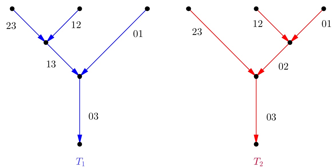
Given a -tree, by fixing the anticlockwise orientation of , we have cyclic ordering of all the semi-infinite edges. We can label connected components of by integers in anticlockwise ordering, inducing a labelling on edges such that edge labelled with will be lying between components and with the unique normal to pointing in component . The labelling can be fixed uniquely by requiring the outgoing edge to be labelled by . For example, there are two different topological types for -trees, with corresponding labelings for their edges as shown in the following figure 1.
Notations 3.
A pair , with being an edge (either finite or semi-infinite) and being an adjacent vertex, is called a flag. The unique vertex attached to the outgoing semi-infinite edge is called the root vertex.
For the purpose of Morse homology, we need the following notation of metric trees.
Definition 4.
A metric -tree is a -tree together with a length function .
Metric -trees are identified up to homeomorphism preserving the length functions. The space of metric -trees has finite number of components, with each component corresponding to a topological type . The component corresponding to , denoted by , is a copy of , where is the number of internal edges and equals to . The space can be partially compactified to a manifold with corners , by allowing the length of internal edges to be infinity. In particular, it has codimension- boundary
where the equation means splitting the tree into and at an internal edge.
2.1.2 Morse structure
We are going to describe the product of the Morse category. First of all, one may notice that the morphisms between two objects and is only defined when is Morse. Given a sequence such that all the difference ’s are Morse, with a sequence of points such that is a critical point of , we have the following definition of gradient flow tree.
Definition 5.
A gradient flow tree of with endpoints at is a continuous map such that it is an upward gradient flow lines of when is restricted on the edge labelled , the incoming edge begins at the critical point and the outgoing edge ends at the critical point .
We use to denote the moduli space of gradient trees (in the case , the moduli of gradient flow line of a single Morse function has an extra symmetry given by translation in the domain. We will use this notation for the reduced moduli, that is the one after taking quotient by ). It has a decomposition according to topological types
This space can be endowed with smooth manifold structure if we put generic assumption on the Morse sequence, which will be described as follows. For an incoming critical point , with corresponding stable submanifold , we define a map
Fixing a point in together with a metric tree , we need to determine a point in . First, suppose is the vertex connected to the edge labelled , there is a unique sequence of internal edges connecting to the root vertex . To determine the image of under our function, we apply Morse gradient flow with respect to Morse function associated to ’s for time to consecutively according to the sequence .
The maps are then put together to give a map
| (2.1) |
where we use the embedding for the first component.
Definition 6.
A Morse sequence is said to be generic if the image of intersects transversally with the diagonal submanifold , for any sequence of critical points and any topological type .
When the sequence is generic, the moduli space is of dimension
where is the Morse index of the critical point. Therefore, we can define , or simply denoted by , using the signed count of points in when it is of dimension . In order to have a signed count, we have to fix an orientation of the space which will be discussed later in definition 40.
We now give the definition of the higher products in the Morse category.
Definition 7.
Given a generic Morse sequence with sequence of critical points , we define
by
| (2.2) |
when
Otherwise, the is defined to be zero.
2.2 Witten’s twisted de Rham category
Given a compact oriented Riemannian manifold , we can construct the de Rham category depending on . Objects of this category are again smooth functions, while the space of morphisms between and is
with the twisted differential , where . The composition of morphisms is defined to be the wedge product of differential forms on . This composition is associative and hence the resulted category is a dg category. We denote the complex corresponding to by and the differential by .
To relate and , we need to apply homological perturbation to . Fixing two functions and , we consider the Witten Laplacian
where . We denote the span of eigenspaces with eigenvalues contained in by .
If the function is a Morse-Smale function (see definition 1), it is proved in [2, Appendix: On the Thom-Smale complex] that the closure and have a structure of submanifold with conical singularities. Using this result, one can define the following map as in [18, 8]
given by
| (2.3) |
which is an isomorphism identifying with Morse differential when large enough.
Remark 8.
This identification gives a connection on the family of vector space parametrized by by declaring the basis associated to critical point of to be flat. Equivalently, it is the same as defining
for , where is the idempotent associated to the orthogonal projection on .
It is natural to ask whether the product structures of two categories are related as , and the answer is definite. The first observation is that the Witten’s approach indeed produces an pre-category, denoted by , with structure . It has the same class of objects as . However, the space of morphisms between two objects , is taken to be , with being the restriction of on the eigenspace .
The natural way to define for any three objects , and is the operation given by
is the idempotent associated to the orthogonal projection to .
Notice that is not associative, and we need a to record the non-associativity. Suppose that is the Green’s operator corresponding to Witten Laplacian , we let
| (2.4) |
and
| (2.5) |
Then is a linear operator from to such that
Namely is a homotopy retract of with homotopy operator . Suppose , , and are smooth functions on and , the higher product
is defined by
| (2.6) |
In general, the construction of can be described using -tree. For , we decompose , where runs over all topological types of -trees.
is an operation defined along the directed tree by
-
(1)
applying wedge product to each interior vertex;
-
(2)
applying homotopy operator to each internal edge labelled ;
-
(3)
applying projection to the outgoing semi-infinite edge.
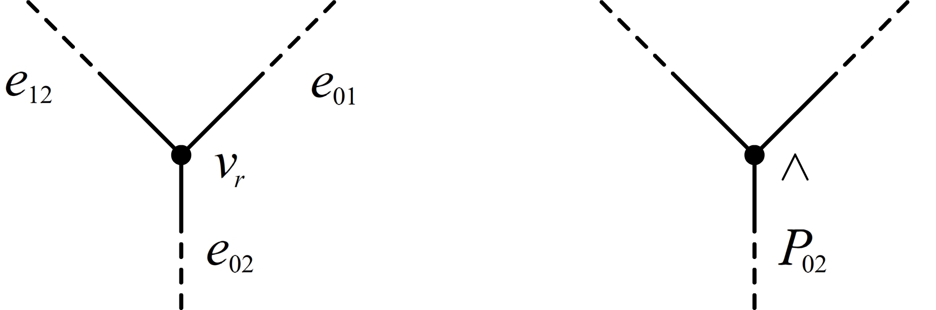
The following graph shows the operation associated to the unique -tree.
The higher products satisfies the generalized associativity relation, called relation. One may treat the product as a pullback of the wedge product under the homotopy retract . This proceed is called the homological perturbation lemma. For details about this construction, readers may see [14]. As a result, we obtain an pre-category .
With the above notations, we restate our main theorem as the following:
Theorem 9 (Main Theorem).
Given smooth functions satisfying the generic assumption in definition 6, with be corresponding critical points, there exist and , such that for all , is an isomorphism when . Furthermore,
with .
Remark 10.
The constants and depend on the functions . In general, we cannot choose fixed constants such that the above statement holds for all and all sequences of functions.
Remark 11.
We would like to emphasize the relation between the main theorem and SYZ Mirror Symmetry. Let be the cotangent bundle of a manifold which equips the canonical symplectic form , and let be Lagrangian sections. Then a critical point of can be identified with . Applying the theorem of Fukaya-Oh [7], the Morse operation is equivalent to Floer theoretical operations counting holomorphic disks. In the simplest situation concerning , the Witten’s twisted de Rham category is related to the Floer theory on via our main theorem 9 and Fukaya-Oh’s theorem. In more general situation, one expects the correspondence will be one of the ingredients for realizing HMS geometrically.
3 Proof of Main Theorem
We fix a generic sequence of functions, with corresponding sequence of critical points . First of all, we have
so is non-trivial only when the equality
| (3.1) |
holds, which is exactly the condition for in the Morse category to be non-trivial. We will therefore assume condition (3.1) and consider the integral
Recall that each directed tree gives an operation and which is also the case in Morse category. Therefore, we just have to consider each separately.
3.1 Results for a single Morse function
We start with stating the results of Witten deformation for a single Morse function which we will assume it to be Morse-Smale as in definition 1. These results come from [11, 12, 13, 18], with a few modifications to fit our content. We introduce the Agmon distance and lemma 13 is just [13, Lemma A2.2].
Definition 12.
For a Morse function , the Agmon distance , or simply denoted by when no confusion occurs, is the distance function with respect to the degenerated Riemannian metric , where is the background metric.
Lemma 13.
We have with equality holds if and only if is connected to via a generalized flow line with and . Here a generalized flow line means that is continuous, and there is a partition such that is a reparameterization of a gradient flow line of and for .
Readers may see [10] for more of its basic properties. The Agmon distance is closely related to the Witten’s Laplacian, or more preciely the corresponding Green’s operator associated to it by the following lemma which is a variant of [12, Proposition 2.2.5] in our current situation (readers may also see [4, Proposition 6.5]).
Lemma 14.
Let to be a subset whose distance from is bounded below by a constant. For any and , there is and such that for any two points , there exist neighborhoods and (depending on ) of and respectively, and such that for any we have
| (3.2) |
for all and , where refers to the Sobolev norm.
We will also need modified version of the resolvent estimate for , which can be obtained by applying the original resolvent estimate to the the formula
| (3.3) |
Lemma 15.
For any and , there exist and such that for any two points , there exist neighborhoods and (depending on ) of and respectively, and such that
| (3.4) |
for all and , where refers to the Sobolev norm.
Under the Morse-Smale condition, one can prove the following spectral gap in the twisted de Rham complex which follows from [13, Lemma 1.6] and [13, Proposition 1.7].
Lemma 16.
For each , there exist and constants such that
for .
Recall that in Section 2.2 we have denoted the subspace of with eigenvalues lying in by , and it is closely related to the Morse complex introduced in Section 2.1.
Furthermore, we have the following theorem on Witten deformation on the level of chain complexes which is [18, Theorem 6.9] in our current situation.
Notations 18.
We will denote the inverse by and write for a critical point of .
Since we are dealing with the case that the background metric which is not flat near critical points of , we will need a combination of techniques from [13, 18] to prove Theorem 17, which we will briefly indicate as follows. Readers may take this part for granted, skip the following section 3.1.1 and go directly into section 3.1.2.
3.1.1 Sketch of proof for Theorem 17 using results from [13]
We use to denote the set of critical points of with being the degree of the critical point. For each , we let
where is the open ball centered at with radius with respect to the Agmon metric, and is a manifold with boundary when is sufficiently small.
For each , we use to denote the space of differential -forms with Dirichlet boundary condition, with Witten Lacplacian acting on it. The spectral gap Lemma 16 holds for as well and since there is only one critical point of degree in , the eigenspaces of with small eigenvalues is -dimensional. We have the following decay estimate which is [13, Theorem 1.4].
Lemma 19.
For any , small enough, we have such that when , has one dimensional eigenspace in . If we let be the corresponding unit length eigenform, we have
| (3.5) |
where stands for bound with a constant depending on . Same estimate holds for any -th derivative as well.
We construct , depending on and as follows. For each critical point , we take a cut off function such that in and compactly supported in . Given a critical point , we let
Definition 20.
For sufficiently small and large , we define
| (3.6) |
where is the idempotent associated to the projection to the small eigenspace.
The difference between and is computed in [12, Lemma 2.1.1], which shows that satisfies the same estimate in Lemma 19. Furthermore, [13, Proposition 1.3] (reader may also see [4, Theorem 3.6]) together with [11, Theorem 5.8] lead the following WKB approximation of (see remark 27).
Lemma 21.
For small enough and large enough, there is a WKB approximation of of the form
| (3.7) |
in a neighborhood of .
Lemma 19, the WKB approximation in the above Lemma 21 combines together with the explicit description of the leading term in [13, Theorem 2.5] and it gives us the explicit computation of as follows.
Lemma 22.
For sufficiently small and large , we have . Suppose that we renormalize , then we have
where if and with
from the Morse-Smale condition.
In particular, if we define by , then we have with for some . This tells us that is an isomorphism when is large enough and is an approximation of .
3.1.2 Exponential decay of
For a critical point , has certain exponential decay measured by the Agmon distance from the critical point as in lemma 23. It is also a consequence of lemma 19 and lemma 22.
Lemma 23.
For any , there exists such that for , we have
| (3.8) |
and the same estimate holds for the derivatives of . Here, refers to the dependence of the constant and .
Remark 24.
We write and which are nonnegative smooth functions with zero sets and respectively, and Bott-Morse in a neighborhood of . More properties of the functions can be found right below [13, equation (2.8)]
In this case, we write
Furthermore, we notice that the normalized basis ’s are almost orthonormal basis as in the following lemma, which is a direct consequence of lemma 23.
Lemma 25.
There exist and such that when such that
3.1.3 WKB approximation for
Restricting on a sufficiently small neighborhood containing , the above decay estimate of ’s from [13] can be improved from an error of order to for an arbitrary which follows from a similar WKB approximation in lemma 21.
Lemma 26.
There is a WKB approximation of of the form
| (3.9) |
in a neighborhood of .
Remark 27.
The precise meaning of this WKB approximation is given in section 4.6. Roughly speaking, it is a approximation in order of on every compact subset of .
Furthermore, the integral of the leading order term in the normal direction to the stable submanifold is computed in [13, Theorem 2.5].
Lemma 28.
Fixing any point and a cutoff function such that around compactly supported in , we take any closed submanifold (possibly with boundary) of intersecting transversally with at . Then, we have
Similarily, we have
for any point , with intersecting transversally with at .
So far we have been considering a fixed Morse function . From now on, we will consider a fixed generic sequence with corresponding sequence of critical points as in the beginning of section 3.
Notations 29.
We use to denote a fixed critical point of . associated to is abbreviated by .
We will use the result in the previous section to localize the integral
| (3.10) |
to gradient flow trees, when the degree condition (3.1) holds.
3.2 Proof of
3.2.1 Apriori estimate for case
We begin with the simplest case which does not involve any homotopy operator . There is an unique -tree with a unique vertex as shown in Figure 2. According to the combinatorics of , we define which is given by
It can be treated as the length of the geodesic tree of type with unique interior vertices and end points of semi-infinite edges ’s laying on ’s.
By lemma 13, we learn that and equality holds if and only if is connected to through a generalized flow line of . Notice that where
| (3.11) |
and the equality holds if and only if is one of the interior vertices of a gradient flow tree of the type . We will only consider gradient flow trees instead of 222Here generalized gradient trees refers to continuous map from to such that the restriction to each edge being a generalized gradient flow line mentioned in lemma 13generalized gradient trees since we assume the sequence of Morse functions satisfies the generic assumption as in definition 6.
Fixing and sufficiently small , we apply cutoff function supported in and obtain
Here the decay factors , and come from the a priori estimate in lemma 23 for the input forms , and respectively.
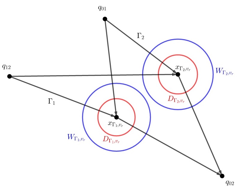
We assume there are gradient trees of the type . For each tree , we take open neighborhoods and of interiors vertices with as shown in following Figure 3.
Since is a continuous function in attending minimum value exactly at internal vertices of gradient trees ’s, we have a constant , depends on the size of the neighborhood ’s, such that in by continuity from the discussion above equation (3.14).
If is away from the ’s, we have
and thus contributes exponentially small error terms.
To obtain the leading order term contribution, we take cutoff functions , associating to each tree , with supports in and equal to on , and get
This localizes the integral computing to gradient trees ’s of type . Notice that the neighborhoods and can be chosen to be arbitrarily small.
3.2.2 WKB methods for
In this section, we introduce the WKB method which allows us to compute the leading order contribution in explicitly. We fix a gradient tree as in the section 3.3.1, with interior vertices (since the gradient tree is fixed, we omit the dependence on in our notations). We take neighborhoods of , with cutoff functions supported in as in section 3.2.1.
As , we can assume that the WKB approximations from lemma 26
hold in for (by lemma 26, for any , we have when is odd, but we still insist to write the expansions in the above form to unify our notations in the rest of the proof), by taking a smaller if necessary while using the lemma 23.
Computing the integral by using the WKB expansions, we have
| (3.13) |
modulo terms of order . We observe that the exponential decay factor of the integrand is , where are introduced in remark 24.
Recall that , and are Bott-Morse with absolute minimums on , and respectively. The generic assumption (definition 6) of the sequence indicates that , and intersect transversally at which means concentrates at . The leading order contribution will be computed in the up coming section.
3.2.3 Explicit computations for
We will need the following lemma which will be proven in section 4.8.
Lemma 30.
Let be a -dimensional manifold and be a -dimensional submanifold in , with a neighborhood of which can be identified as the normal bundle . Suppose is a Bott-Morse function with zero set and has a vertically compact support along the fiber of , we have
where is the integration along fiber and is the volume polyvector field defined for the positive symmetric tensor along fibers of .
From lemma 30, we know that the leading order contribution in the above integral (3.13) depends only on values of , and at the point . We use the normal bundle at to parametrize a neighborhood of . Making use of lemma 30, we can split the integral as follows for computing leading order contribution. We have
where the sign depends on whether the orientations of and match or not at the point . From lemma 28, we obtain equality
for and
from the lemma 28. Therefore we conclude that
where the sign depends on matching the orientations of and at the point .
Remark 31.
Notice that we have a stronger estimate with the error term being instead of since the estimate of the homotopy operator (see lemma 32) is not involved in the case.
3.3 Proof of
Next we consider the case to illustrate the analytic argument needed for handling the homotopy operator .
3.3.1 Apriori estimate for case
There are two -leafed directed trees, which are denoted by and . We simply consider where is the tree shown in figure 1 and relate this operation to counting gradient trees of type . has two interior vertices and . According to the combinatorics of , we define by
It is the length of the geodesic tree of type with interior vertices and endpoints of semi-infinite edges ’s laying on ’s as shown in the following figure.
![[Uncaptioned image]](/html/1401.5867/assets/gradtreelength.jpg)
Similar to the proof of case in section 3.2, we notice that where
| (3.14) |
and the equality holds if and only if are interior vertices of a gradient flow tree of the type . Once again we only have gradient flow trees instead of generalized gradient trees since we assume the sequence of Morse function satisfyies the generic assumption (see definition 6).
Fixing two points and sufficiently small such that estimate for as well as in lemma 15 holds for some balls and (with respect to ). If and are cutoff functions supported in and respectively, then we have
for those large enough , where lemma 23 gives the decay factors and of the input forms and respectively, and lemma 15 gives the decay factor . Combining with the decay estimates for and as in section 3.2, we obtain
where are the centers of balls chosen for taking the cutoff functions as above and is defined in equation (3.14).
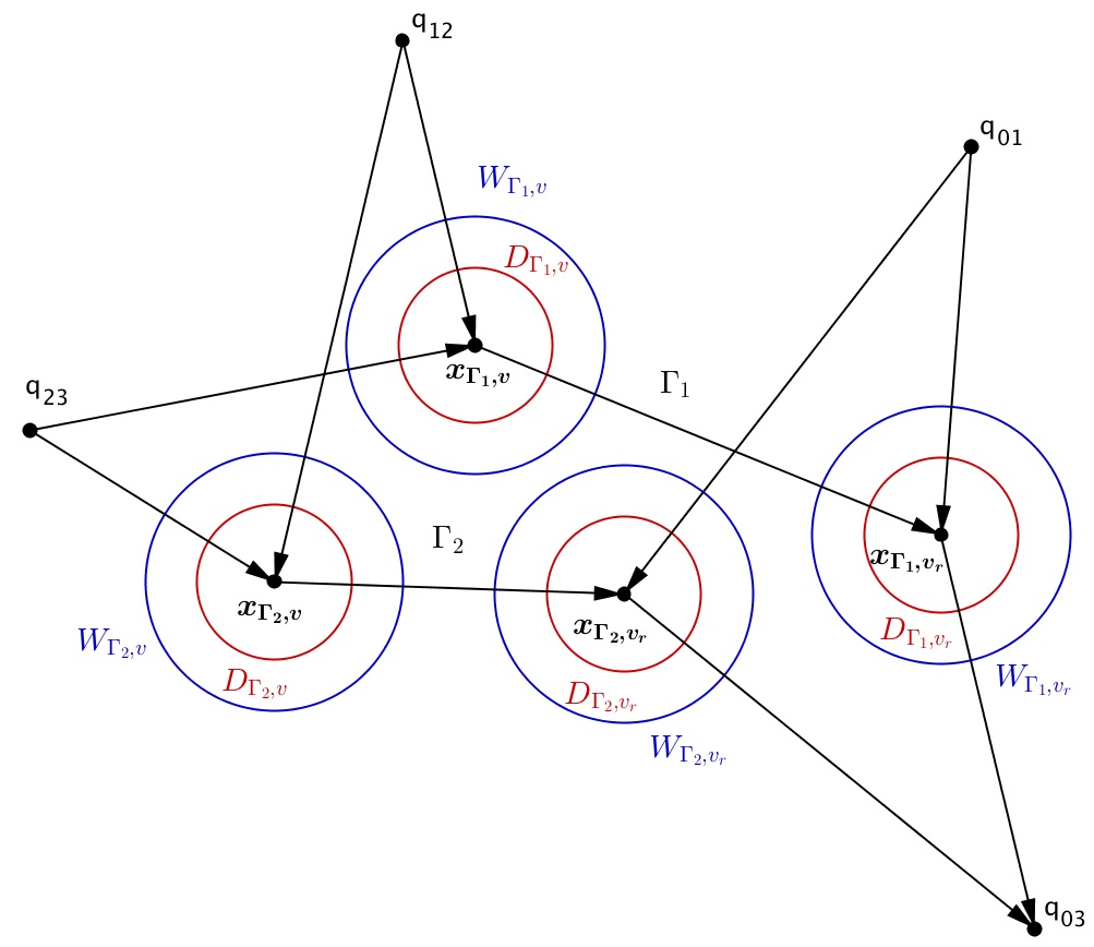
Once again we assume there are gradient trees of the type . For each tree , we take open neighborhoods and of interiors vertices with , and similarly and for , as illustrated in figure 4.
Since is a continuous function and it attends minimum value exactly when for some gradient tree , there is a constant (again depending on the size of the neighborhood ’s) such that in by continuity from the discussion at the beginning of section 3.3.1, where .
If is away from the ’s, we have
Therefore we can take cutoff functions , associating to each tree , with supports in , and equal to on , respectively, and obtain
This localizes the integral computing to gradient trees of type where the neighborhoods and can be chosen to be arbitrarily small.
3.3.2 WKB method for
Similar to the previous section 3.2.2, we only focus on a gradient tree of type as in the section 3.3.1, with interior vertices and . Once again, we omit the dependence on to simplify our notations. We take neighborhoods and of and respectively, and and are cutoff functions supported in and respectively as shown in the following figure.
![[Uncaptioned image]](/html/1401.5867/assets/wkbgradtree.jpg)
As , we can assume that the WKB approximations from lemma 26
and
hold in (indeed and when is odd), by taking a smaller if necessary while using the lemma 23. Then, we need a similar WKB approximation for the term
in the neighborhood . Here we state a WKB lemma for the homotopy operators which appear in the higher products for . The proof will occupy the whole section 4.
WKB for homotopy operator
Let be a flow line of starts at and ends at for a fixed . We consider an input form defined in a neighborhood of . Suppose we are given a WKB approximation of in , which is an approximation of according to order of of the form
| (3.16) |
(The precise meaning of this infinite series approximation can be found in section 4.6). We further assume that is a nonnegative Bott-Morse function in with zero set . We consider the equation
| (3.17) |
where is a cutoff function compactly supported in , is the projection. We want to have a WKB approximation of the solution to the equation (3.17).
Lemma 32 (=Theorem 68).
If is small enough, there is a WKB approximation of in a small enough neighborhood of , of the form
| (3.18) |
Furthermore, is a nonnegative Bott-Morse function in with zero set which is closed in , where is the time flow of (normalized according to ).
WKB for (cont’d)
We apply lemma 32 with Morse function , input form , starting vertex , ending vertex , with neighborhood and (This can be done by shrinking and if necessary). As a result, we obtain the WKB approximation
by taking and in the lemma.
In order to compute
up to an error of order , we can simply compute the integral
| (3.19) |
We study the exponential decay factor of the integrand by defining . Then, the exponential decay of the integrand can be expressed as
Once again remark 24 tells us that , , and are Bott-Morse with absolute minimums on , , and respectively. We also recall from lemma 32 that is a Bott-Morse function in with absolute minimum denoted by (colored red in the following figure), which is the submanifold flowed out from (colored blue in the following figure), under the flow of which is denoted by .
![[Uncaptioned image]](/html/1401.5867/assets/homotopysubman.jpg)
The generic assumption of the sequence indicates that , and intersect transversally at which means concentrates at and hence the leading order contribution will only depend on the value of at the point .
3.3.3 Explicit computations for
From lemma 30, we know that the leading order contribution of the integral (3.19) depends only on values of , and at the point and the integral can be splitted as
where the sign depends on whether the orientations of and match or not at the point . We will compute the above integrals one by one. We obtain equality
and
from the lemma 28. Moreover, we have
This depends on the fact that
and the following lemma.
Lemma 33 (=Lemma 70).
Using same notations in lemma 32 and suppose and are cutoff functions supported in and respectively, then we have
| (3.20) |
Furthermore, suppose , we have . Here refers to for a rank vector bundle .
Putting the above together, we get the following
| (3.21) |
where the sign depends on matching the orientations of and at the point . The proof for is completed and we move on to the case for any . The proof is essentially the same as the case except involving more combinatorics and notations.
3.4 Proof of
3.4.1 A priori estimates for
We fix a -leafed tree and denote the corresponding operation by . We try to relate to counting of gradient trees of type . Firstly, we define the function according to the combinatorics of by
| (3.22) |
Here the variables are labelled by the vertices of . ( and refer to the variables corresponding to vertices which are starting point and endpoint of the edge respectively.) Recall that is the set of internal edges of and each interior edge has a unique label by two integers as , corresponding to the Morse function . The notation refers to the Agmon distance corresponding to the Morse function .
is the length function of a geodesic tree (may not be unique) with topological type , with interior vertices and semi-infinite edges ended at critical points . Similar to the case of , we have the following lemma.
Lemma 34.
The function is bounded below by , and it attains minimum at if and only if is the vector consisting of interior vertices of a gradient flow tree of of type ended at the corresponding sequence of critical points .
Proof.
Similar to the case, every gradient flow tree is associated with a unique minimum point of . For each tree, we take a covering of , given by a product , where each is an open subsets in containing such that all ’s are disjoint from each other. If we further take such that , we have a constant depending on size of ’s such that on (here is the constant in the lemma 34). We are going to localize the integral (3.10) as follows.
We take a finite covering of with balls of radius centering at , with a partition of unity subordinating to it. We choose a covering of given by product , where . We decompose such that is empty for all and for all . These can be achieved by choosing sufficiently small .
We can take cutoff functions subordinating to the covering , given by product of functions on . We write which is a function supported in . We will use to cut off the following integral
| (3.23) |
Recall that the is defined by using wedge product and the homotopy operators and the combinatorics of the tree . We cut off the operation using the function whenever taking wedge product at the vertex . We will write for the integral after cutting off by . Therefore we have
| (3.24) |
where stand for operation after cutting off by . Recall that there is a unique root vertex associated to the direct tree , by applying the resolvent estimate in lemma 15 and the estimate in lemma 23, we obtain the following:
Lemma 35.
For any , there exist such that if we take the covering of radius , we have
| (3.25) |
for any , where is the center of the ball .
The proof is essentially the same as the case for . Similarly, we have
for sufficiently large . It follows from the fact that for those covering in . This result basically says that the integral can be localized to gradient flow tree using the cutoff mentioned above. To summarize, we have the following proposition.
Proposition 36.
For each gradient flow tree , there is a sequence of cutoff functions which is supported in and satisfies on such that
when is sufficiently large.
Remark 37.
In the above argument, the neighborhood can be chosen to be arbitrary small. We will obtain a smaller constant if we shrink the neighborhood .
After localizing the integral, we move on to the section concerning WKB approximation which helps to compute of the leading order contribution of .
3.4.2 WKB method for
We consider a gradient tree of type , with semi-infinite incoming edges. Recall in section 2.1.1 that each edge in is assigned with a label by two integers and . We will use to represent an edge in and denote the corresponding edge in the gradient tree by . The vertex in the gradient tree corresponding to in will be denoted by . We again omit the dependence on in our notations as it is already fixed. We are going to associate , together with its WKB approximation
in some neighborhood of to each flag as shown in the figure 5. We also fix cutoff functions supported in and study the integral using the arguments in section 3.3.1.

We define the followings inductively.
-
(1)
for a semi-infinite incoming edge which ends at vertex , we take to be the input , with its WKB approximation in as in lemma 26. We also let . We also choose to be small enough so that the WKB approximations of all input forms associated to edges connected to holds in ;
-
(2)
for an internal edge which starts at vertex , must be the endpoint of edges and as shown in figure 6,
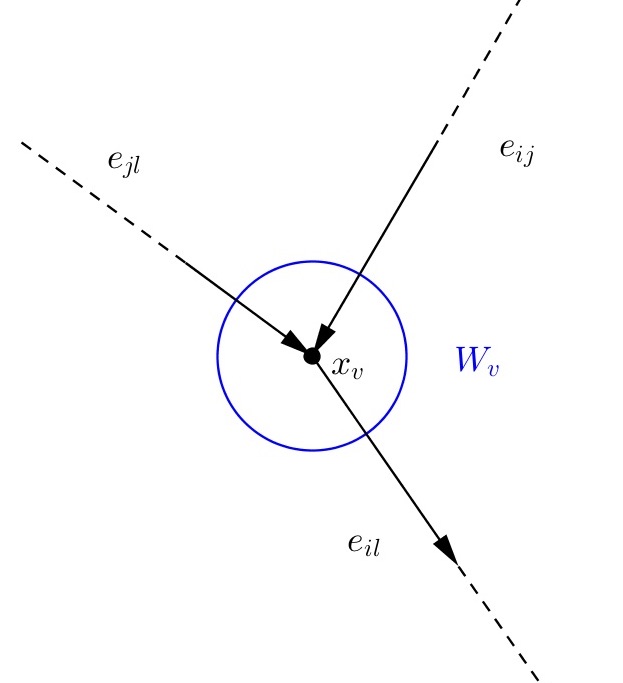
Figure 6: we take . The WKB expression of is defined by the following equations:
We also let ;
-
(3)
for an internal edge with its starting vertex and ending vertex as shown in figure 7,
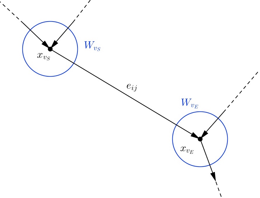
Figure 7: we define in and the corresponding WKB approximation can be obtained from lemma 32 if and are chosen to be small enough. We also define and .
-
(4)
for the semi-infinite outgoing edge with the root vertex , we take to be the form , with WKB approximation from lemma 26. We also define .
Remark 38.
From the definition of , we see that
if three edges , and are meeting at the root vertex . Applying lemma 26 to input forms and lemma 32 to homotopy operators along internal edges , we prove that each WKB approximation
is an approximation with error for arbitrary . Therefore, we can replace each by the first term in its WKB approximation for computing the leading order contribution. We obtain
| (3.26) |
3.4.3 Explicit computation for
The argument of the general case is similar to the case , with more combinatorics involved. Similar to the previous section, we may drop the dependence of in our notations. We are going to show that
| (3.27) |
where the sign agrees with that associated to the gradient tree in Morse category. We begin with some notations associated to .
Notations 39.
Given a gradient tree , we inductively associate to each flag an oriented closed submanifold by specifying orientation of its normal bundle. We require:
-
(1)
for each semi-infinite incoming edge with ending vertex , we let , where is the stable submanifold of from the critical point with the chosen orientation equals to that in the Morse category;
-
(2)
for an internal edge with its starting vertex and assume and are two incoming edges meeting at as in figure 6. We let (the intersections is transversal from the generic assumption) and , if and are two corresponding orientation forms;
-
(3)
for an internal edge with its starting vertex and ending vertex , we define to be obtained from applying lemma 32 to the homotopy operator . The orientation form is chosen such that , under the identification by flow of ;
-
(4)
for the semi-infinite incoming edge with root vertex , we let , where is the unstable submanifold of from critical point with the chosen orientation equal to that in the Morse category.
We further choose an isomorphism and projection map for every flag
| (3.28) |
by further shrinking suitably.
We can therefore assign a sign to the gradient tree in the following way.
Definition 40.
For a generic sequence of Morse functions with corresponding critical points satisfying the degree condition (3.1), which gives a gradient tree , we define
| (3.29) |
where and are edges joining the root vertex as in section 6, is the orientation of normal bundle defined in notation 39 and is the orientation of chosen for .
We are going to show that
for any flag except the outgoing edge , where is the number of internal edges before the vertex . This can be seen inductively along the tree . We see that:
We can now calculate the leading contribution from the integral (3.26). Recall that we have
| (3.30) |
Therefore we obtain
which means
| (3.31) |
The sign comes from matching the orientation against that of , which agrees with the sign in Morse category. This completes the proof of our main theorem.
4 WKB for Green operator
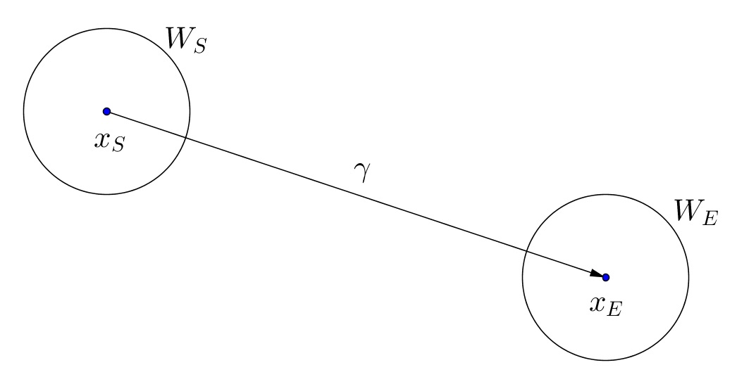
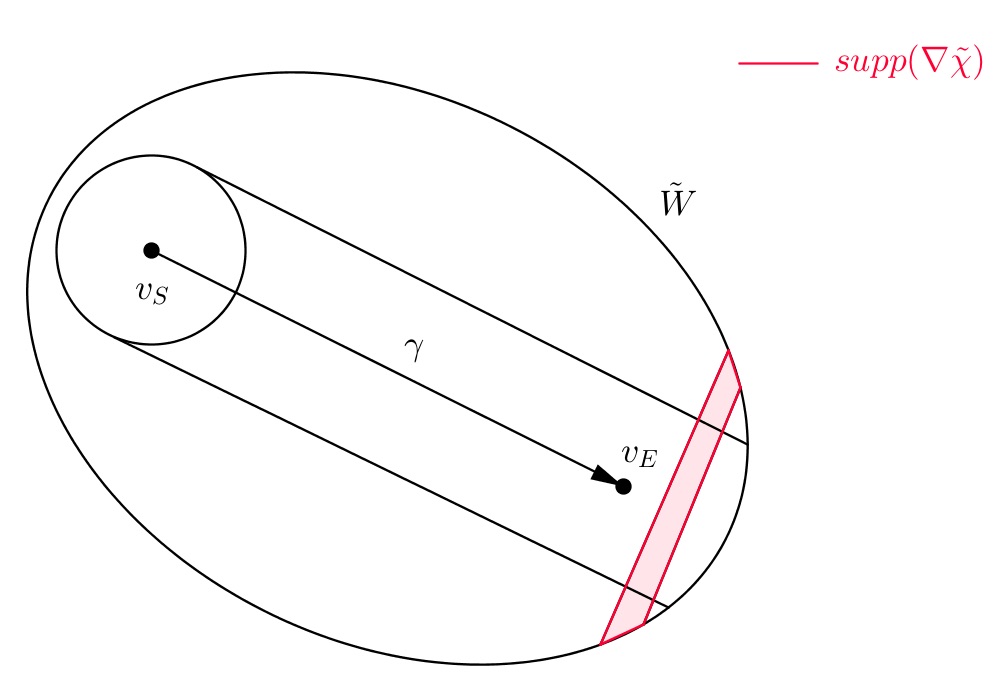
In lemma 15, we have a rough estimate for the twisted Green operator by a Morse function , or the homotopy operator , with an error of order . In a neighborhood of the gradient flow line segment of , we are going to improve this results to estimate with error for an arbitrary . This is done by the WKB method for inhomogeneous Laplace equation (3.17).
We study the local behavior of the homotopy operator along a normalized gradient flow line segment
| , |
with along , as shown in figure 8.
Suppose that and we have a WKB approximation of in of the form
| (4.1) |
we aim at establishing a similar expression
| (4.2) |
of in some open neighborhood of . It is possible to propagate the estimate along since along .
The key step is to determine , which is given in the following subsection. As the first trial, we consider the function
since is the expected exponential decay suggested by the resolvent estimate in lemma 15.
Unfortunately, is not the correct choice since it is singular along a hypersurface through , and it cannot be used for the iteration process as we keep on differentiating it.
In the coming section 4.1, we will solve the minimal configuration in variational problem associated to and find that the point must lie on , with a unique geodesic joining which realizes , for those closed enough to . These family of geodesics gives a foliation of a neighborhood of . Therefore we can use as an extension of across . We then use in the iteration similar to classical WKB approximation to obtain the above expansion (4.2).
4.1 The phase function
We apply variational method to study the function . Fixing , we define such that for all . To minimize the functional
we take derivative and get
Lemma 41.
(First variation formula)
| (4.3) |
Here is the Levi-Civita connection corresponding to the Agmon metric in definition 12.
If we assume is a geodesic (with respect to twisted metric ) with being constant, the Euler-Lagrange equation for is
Since can be chosen arbitrarily, we have
| (4.4) |
Such an equation restricts the possibility of the starting point , namely, we have
at , or equivalently, .
Definition 42.
If is a local extrema of with , it forces . To obtain nice properties of , we are going to assume the following throughout the whole section.
Assumption 43.
We define by and assume it to be a smooth Bott-Morse function in with critical point set which contains .
Lemma 44.
is a hypersurface containing if (we shrink if necessary). Otherwise, it is simply .
Proof.
Since we have on and hence on . This gives . Moreover, can be defined by the equation
If where , then we have
since on . As is a Bott-Morse function with critical set , is nondegenerate when it is restricted on the orthogonal complement of in . Therefore, there exists such that . ∎
We are going to parametrize a neighborhood of by such that is an embedding and is . is defined to be the coordinate function corresponding to the last variable.
Motivated from equation (4.4), we define a transversal vector field on which is the initial tangent vector for minimizer of .
Definition 45.
We define a vector field transversal to (shrinking if necessary) by
| (4.5) |
Notice that on .
It follows from the Euler-Lagrange equation (4.4) that any local extrema of will have and . For convenience, we assume that is extended to gradient flow line defined on containing .
Definition 46.
We define a map
| (4.6) |
by
where is a suitable neighborhood of where the exponential map with respect to the Agmon Riemannian metric is well defined.
Lemma 47.
Restricting to a small open neighborhood of , is a diffeomorphism onto its image containing .
This is achieved by showing there is no “conjugate point” along for certain type of geodesic family, and using the fact that being a global minimizer of functional . Lemma 47 enables us to construct needed for WKB approximation in a neighborhood (take a small enough and shrink if necessary) of where is a differeomorphism.
Definition 48.
We define on by
| (4.7) |
for .
4.2 Well-definedness of the phase function
We prove lemma 47 in this section for ensuring the well-definedness of . We begin with the second variation formula of . Assume is a family such that is arc-length parametrized geodesic (with respect to twisted metric ) satisfying the condition
From the first variation formula
we obtain
Lemma 49.
(Second variation formula)
| (4.8) |
where the right hand side is evaluated at . Here is the curvature tensor with respect to .
If we further impose the condition that for all , we have
| (4.9) |
Therefore we consider the bilinear form associated to the above quadratic form.
Definition 50.
| (4.10) |
for vector fields on , .
For any such vector field , we can find a family of curves satisfying the assumption with . The same holds for piecewise smooth vector field with the same initial condition.
Proof of lemma 47.
The proof depends on the fact that is an absolute minimum of among the set of paths in with , and contradiction will occur if the differential of is singular along . This argument is a modification of the standard one of geodesic beyond conjugate point is never length minimizing.
First, we notice that for a fixed . We have to compute for arbitrary . We claim that will never be parallel to for .
Taking a curve in with and , we can construct a family of arc-length parametrized geodesics by taking exponential map
We have with being a Jacobi field on . Suppose the contrary that for some constant , then we must have , otherwise we must have which contradicts .
We claim that there is a path from to the point which gives a smaller value of comparing to the gradient flow line from to the point . We will denote to fit our previous discussion.
We construct the path by defining a variational vector field on , depending on a small to be fixed. We take a vector field such that , , on and . We define a piecewise smooth vector field
where is a cutoff function on with and in a neighborhood of . Notice that from the fact that . A direct computation shows
We have for small enough.
By taking the family of curves corresponding to , we obtain
where . For small enough , will be a curve from to which gives a smaller value of comparing to . This is impossible because we have
and the lower bound is attained at .
As a conclusion, we can show that gives a local diffeomorphism onto its image by shrinking if necessary. Therefore it is injective in a contractible neighborhood of the gradient flow line . ∎
Under the identification , we use the coordinate for and use , or simply , as coordinates for image of under . By shrinking if necessary, we assume that is a coordinate chart through the map . This justifies definition 48 of being a smooth function on .
4.3 Properties of
We are going to study the first and second derivatives of which is necessary for WKB approximation in the equation (3.17). We define
as shown in the following picture.
![[Uncaptioned image]](/html/1401.5867/assets/fig_2.jpg)
Lemma 51.
In , we have
In particular, we have on and .
Proof.
We first consider the subset in . Let be a curve in such that and
Notice that we have . Applying the first variation formula, we have
As can be chosen arbitrarily, we get
The same argument works for by taking
Furthermore, we have which gives . Finally, as we know on and flow lines of are geodesics after reparametrizations, we get on . ∎
We now consider the second derivatives of .
Lemma 52.
By choosing a small enough , we have
-
1.
and
-
2.
is a Bott-Morse function with critical set .
Proof.
The previous lemma implies that on . We are going to show is positive definite in the normal bundle of . Fixing any , we consider the submanifold . There is an isomorphism between the normal bundle of in and the normal bundle of in . Therefore we restrict on and consider its Hessian.
We abuse the notations and write as the projection map. We take , then on by definition of and on . Therefore we have is positive semi-definite on the normal bundle of in . Moreover, we have on being positive definite in the normal bundle.
By choosing sufficiently small , we can assume that along and hence the result follows. ∎
Next, we consider the second order derivatives for defined on .
Lemma 53.
By choosing small enough neighborhood of if necessary, we have
-
1.
on and
-
2.
is a Bott-Morse function with critical set .
Proof.
We first have on because on . If we consider on , then we have and . Therefore, there exists an neighborhood of in so that
for all . Choosing small enough will achieve the desired result. ∎
Remark 54.
We can extend the function from to to be a non-negative function with critical set which is also an absolute maximum. This is for our convenience in later arguments.
4.4 The WKB iteration
After knowing these properties of , we will describe the iteration procedure to define inductively.
First, by lemma 51, we have and hence the expansion
where . Following [13], we let
and consider the following equation
order by order in where is a function (depending on ). We often write to simplify our notations. The first equation to be solved is
| (4.11) |
In order to solve the above equation involving , we need a map describing the flow of . It is given by renormalising such that and is of the form
| (4.12) |
with the same image as . We can also assume that is a connected open interval.
Notations 55.
We use as coordinates of from now on. For simplicity, we also let and .
For the iteration process, we focus on
for the definition of the following integral operator.
Definition 56.
We let given by
| (4.13) |
where is the flow of for time .
4.5 Estimate of the WKB iteration
In this section, we are going to obtain norm estimates for ’s. We consider terms appearing in the iteration which are essentially of the form
| (4.18) |
with and , where is the composition of for times. Here each is a multi-index such that
With
we have
| (4.19) |
for from lemma 53.
Remark 57.
Different choices of order of taking differentiation in definition of will result in a difference involving the curvature of , however, the order of vanishing in equation (4.19) remains unchanged and hence the following estimates hold for any such choice.
The counting of vanishing order along is needed for applying the following semi-classical approximation lemma 58, appearing in [4].
Lemma 58.
Let be an open neighborhood of with coordinates . Let be a Morse function with unique minimum in . Let be a Morse coordinates near such that
For every compact subset , there exists a constant such that for every with , we have
| (4.20) | |||||
where
and .
In particular, if vanishes at up to order , then we can take and get
From the above, we obtain the following lemma.
Lemma 59.
Let be the line interval along direction with fixed coordinates, we have the norm estimate
for any multi-index and .
Motivated by the above lemma, we consider a filtration
of the space of differential forms on which is defined as follows.
Definition 60.
is in if for any compact subset and integers , we have
for any line .
The Lemma 59 simply means .
Proposition 61.
We have and , where denotes the wedge product of forms.
Proof.
The first property is trivial. For the relation , we fix and a compact subset . For and , we first observe that
Then the Hölder inequality implies that
and the result follows. ∎
Lemma 62.
For , we have
Proof.
To simplify the notations, we only prove the statement for functions as we can fix a basis (independent of ) for differential forms in , and estimate the coefficient functions. The Christoffel symbols appearing in differentiating the basis will be independent of and not affecting the following estimates. For the same reason, let us simply pick a flat metric in ’s coordinates for simplicity. In that case, we can write .
We first consider the operator , and we will have where is acting as scalar multiplication by function. Therefore we have
This implies .
Next, we consider the operator for . Fixing a multi-index and using the result , we have
which gives .
It remains to show that which requires estimates of the term . There are two cases to be considered, and . If , we can cancel the integral operator with one of the , which gives
where refers to the multi-index by letting .
If , we can commute all the with the integral operator . We let as a function and write . Therefore we have
and
Combining the two cases will give . ∎
Remark 63.
Using the above lemma, we can show that the ’s appearing in the iteration equation (4.17) will satisfy . In particular, we can get an explicit estimate as
for all and compact subset .
4.6 A priori estimate
We make use of the WKB iteration to construct the WKB expansion and prove that it does give a desired approximate as in theorem 68 to the solution in section 4.6 and section 4.7. This is a standard technique which is taken from [11] (readers may also see [9, Chapter 4]), with slight modification in the current case. To begin with, we obtain an a priori estimate for the solution in this subsection.
We consider the equation
| (4.21) |
in , where is the input form depending on and is some cutoff function to be chosen later. We assume has a WKB approximation on of the form
| (4.22) |
where and . It is an approximation in the sense that
| (4.23) |
for large enough, where is a constant depending on . We also require similar norm estimates for its derivatives
| (4.24) |
with depending on .
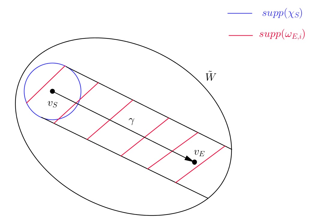
We want to get a similar expansion for , using the iteration defined in the section 4.4. We consider any small enough compact neighborhood of the flow line with on . is chosen so that . The following figure illustrates the situation.
![[Uncaptioned image]](/html/1401.5867/assets/wkb3.jpg)
If is small enough, we have an a priori estimate of in as lemma 64, which is essentially the result of [11, Proposition 5.5] with modification to suit our current situation.
Lemma 64.
For small enough and , and any , there exists such that for any , we have
| (4.25) |
where is an positive integer depending on .
In order to prove the above lemma, we need to know certain properties of and the chosen compact set . Let , we have the following lemma playing the role of [11, Lemma 5.7].
Lemma 65.
There exists such that for all sufficiently small , we have
| (4.26) |
for all and .
Proof.
Using the fact that on and choosing small enough such that on , we can simply prove
by choosing small enough and . From the properties of Agmon distance , we have
with equality holds only if and there is a generalized gradient line joining to . Therefore, we have
with equality holds only if there is a generalized gradient line joining a point to and then to . This is impossible by for our choices of and . Hence we always have strict inequality and therefore we can find small by compactness argument. ∎
We consider a closed neighborhood of in with smooth boundary. We let to be the twisted Green’s operator on using Dirichlet boundary condition. We first argue that can be replaced by .
Lemma 66.
There exists such that
for all whenever and are chosen to be small enough.
Proof.
Next, we obtain estimates for similar to those in lemma 64 for using the argument as in [11, Proposition 5.5].
Lemma 67.
For any , there exists such that if , we have
| (4.28) |
where is an positive integer depending on .
Proof.
We consider the equation
| (4.29) |
with Dirichlet boundary condition in , and divide the proof into three steps:
Step 1: Without loss of generality, we assume there is a constant such that and on . We define the function
| (4.30) |
with to be chosen. Therefore we have
Using the equation (4.29) we get
and if we choose a large to absorb the term , we have
Therefore we get
and so , for .
Step 2: We prove the estimate for derivatives of . We apply and to both sides of equation (4.29). We obtain
| (4.31) |
Applying the result in step to , we have
Since , we have
Corresponding result for can be obtained by a similar argument. These combine together to obtain an estimate for . By applying successively, we obtain all higher derivatives’ estimates in a similar fashion.
Step 3: Finally, we improve the estimate to norm. Since we have norm estimate for all the derivatives of . We use the Sobolev embedding on to obtain the norm estimate. Details are left to readers. ∎
4.7 WKB approximation
Next, we consider the WKB approximation of . From the WKB approximation (4.1) of , we can take on both side and obtain a WKB approximation of
| (4.32) |
after grouping terms according to their orders of . We apply the iteration in the previous subsection 4.4 terms by terms to the above series and then group the terms according to orders of of their norms. As a result, we obtain a WKB expansion
| (4.33) |
in , where ’s are functions also depending on . Using lemma 62 and remark 63, we know that for every and any compact subset ,
for those , and also
for . After establishing the estimate of WKB iteration in section 4.5, we need to show that it is a good approximation as stated in theorem 68. The proof is actually a slight modification of [11, Theorem 5.8].
Theorem 68.
For any and small enough, and large enough, there exists such that for we have
| (4.34) |
Proof.
Making use of lemma 66, we again consider the equation 4.29. It suffices to show that the approximation works for on some small enough pre-compact neighborhood of the flow line . We divide the proof into several steps.
Step 1: As ’s do not vanish on boundary of , we first need to cut them off suitably for applying integration by part. ’s, being defined by integrating along flow of , have support as shown in the following figure 9.
Suppose we have , then we can choose which only depends on variable (using coordinate defined by ) such that for . The support of is shown in the following figure 10.
By shrinking and if necessary, we obtain some such that
| (4.35) |
for and . We define the function
| (4.36) |
where is defined in (4.30), and is chosen as in lemma 65. We have
for large enough. Notice that we have in for large enough, and in .
Step 2: Writing the reminder term as , we get
We handle the right hand side term by term. First, we have
Second, we have
Third, we have
where is the integer in lemma 64. Finally, we have
by choosing a larger independent of , if necessary. Combining the above, by choosing , we have
which gives , for those .
Step 3: We obtain estimate for all derivatives of . We repeat the above argument for and . For any , we can find a large enough such that for any , we have
for .
Step 4: We apply interior Sobolev embedding to improve the statement in step into norm, by further shrinking if necessary. As a result, we have for large enough, there exists and such that we have
| (4.37) |
for . Finally, we observe that and hence obtain the result by dropping redundant terms in the approximation series.
∎
Finally, we restrict on a sufficiently small neighborhood of . Since the operator is given by an integral with an exponential decay along flow line, we can apply lemma 58 to obtain an expansion
By regrouping terms according to their orders of , we obtain an expansion of the form given in equation (4.2).
4.8 Relation between and
From section 4.4, we constructed a WKB approximation in
In particular, is given by
| (4.38) |
In this section, we study the relation between integrals of and which is used in lemma 33. We begin by recalling lemma 30. Let be a -dimensional manifold and be a -dimensional submanifold in , with a neighborhood of which can be identified as the normal bundle . Suppose is a Bott-Morse function with zero set , we have
Lemma 69.
Let which is vertically compact support along the fiber of . Then, we have
where is the integration along fiber and is the volume polyvector field defined for the positive symmetric tensor along fibers of .
We use the notations in section 4.1 and assume there is an identification of and with the normal bundle and of and respectively. We use and to stand for the bundle maps respectively. We have the following lemma which relates the integration of and along the fibers of and respectively.
Lemma 70.
Assume on , then
where is the projection map using the identification given by (flow of ). Furthermore, we have on .
Proof.
We use the coordinates for , where are coordinates of . We further assume that . From lemma 53, is a Bott-Morse function with zero set . Applying lemma 69 to the equation (4.38), we have
modulo terms of . From lemma 52, is a Bott-Morse function with zero set . Applying lemma 69 again, we get, modulo terms of ,
for those . The term involving is dropped as vanishes for . To make further simplifications, we need the following lemma.
Lemma 71.
Fixing a point , we have
as operators on , where the right hand side acts as multiplication. Here is treated as an operator acting on using the metric tensor.
From the fact that upon restricting to , we have for those and
Notice that on , therefore we have
where we view as a -bundle over and consider as the volume vector field along its fibers. Furthermore, we have the relation
Combining the above, we have
Finally, from the relation , we get
on , where is the volume polyvector field along the fibers of . Therefore, we have
modulo terms of , for those . ∎
Proof of Lemma 71.
First of all, we have the equality
on the set . We can treat as an operator acting on as is Morse along . Restricting to , it is just . Therefore we have
acting on .
On , we have
We will show that the above expression vanish.
Restricting on the set , for any vector fields , we have
and
Therefore, we have
where the Hessians are treated as endomorphisms of . Restricting the above equation to the subspace and multipling by , we have
Finally, from the equation , we obtain
Applying to both sides and restricting to , it gives
or simply
if we treat both sides as operators on .
5 Conclusion
From the semi-classical analysis of the Witten twisted Green’s operator in section 4, we obtain our main theorem 9 which can be viewed as an enhancement of the original Witten deformation of de Rham complex, concerning cohomology of the manifold , to one concerning its rational homotopy type by incorporating wedge product structures. In [6], Fukaya proposed a differential geometric approach to the Strominger-Yau-Zaslow (SYZ) by relating A-model holomorphic disks instantons of a Calabi-Yau manifold equipped with Lagrangian torus fibration, to certain Witten twisted differential constructed from the symplectic structure. Proving theorem 9 provides essential analytical technique for such an approach. For instance, the semi-classical analysis of Witten twisted Green’s operator, can be applied to obtain a beautiful geometric interpretation of the complicated scattering diagram in [3].
Acknowledgements: The authors thank Kwokwai Chan, Cheol-Hyun Cho, Yau Heng Tom Wan and Siye Wu for useful discussions. Kaileung Chan would like to thank Siye Wu for his kind hospitality. Ziming Nikolas Ma would like to thank Prof. Shing-Tung Yau for the support during his visit to Yau Mathematical Sciences Center, Tsinghua University. Naichung Conan Leung were supported in part by grants from the Research Grants Council of the Hong Kong Council of the Hong Kong Special Administrative Region, China (Project No. CUHK 402012, Project No. CUHK 14302215 and Project No. CUHK 14303516).
References
- [1] M. Abouzaid, Morse homology, tropical geometry, and homological mirror symmetry for toric varieties, Geom. Topol. 10 (2006), 1097–1157. MR 2529936, Zbl 1204.14019
- [2] J.-M. Bismut and W. Zhang, An Extension of a Theorem of Cheeger and Müller, Astérisque (1992), no. No. 205. MR 1185803, Zbl 0781.58039
- [3] K.-W. Chan, N. C. Leung, and Z. N. Ma, Scattering diagrams from asymptotic analysis on Maurer-Cartan equations, arXiv preprint arXiv:1807.08145 (2018).
- [4] M. Dimassi and J. Sjöstrand, Spectral asymptotics in the semi-classical limit, London Mathematical Society Lecture Note Series, vol. 268, Cambridge University Press, 1999. MR 1735654, Zbl 0926.35002
- [5] K. Fukaya, Morse homotopy, -category, and Floer homologies, Proceedings of GARC Workshop on Geometry and Topology ’93 (Seoul, 1993), Lecture Notes Ser., vol. 18, Seoul Nat. Univ., Seoul, 1993, pp. 1–102. MR 1270931, Zbl 0853.57030
- [6] , Multivalued Morse theory, asymptotic analysis and mirror symmetry, Graphs and patterns in mathematics and theoretical physics, Proc. Sympos. Pure Math., vol. 73, Amer. Math. Soc., Providence, RI, 2005, pp. 205–278. MR 2131017, Zbl 1085.53080
- [7] K. Fukaya and Y.-G. Oh, Zero-loop open strings in the cotangent bundle and Morse homotopy, Asian J. Math. 1 (1997), no. 1, 96–180. MR 1480992, Zbl 0938.32009
- [8] F. R. Harvey and H. B. Lawson Jr, Finite volume flows and Morse theory, Ann. of Math. (2) 153 (2001), no. 1, 1–25. MR 1826410, Zbl 1001.58005
- [9] B. Helffer, Semi-classical analysis for the Schrödinger operator and applications, vol. 1336, Springer, 2006. MR 0960278, Zbl 0647.35002
- [10] B. Helffer and F. Nier, Hypoelliptic estimates and spectral theory for Fokker-Planck operators and Witten Laplacians, Lecture Notes in Mathematics, vol. 1862, Springer-Verlag, Berlin, 2005. MR 2130405, Zbl 1072.35006
- [11] B. Helffer and J. Sjöstrand, Multiple wells in the semi-classical limit I, Comm. in PDE 9 (1984), no. 4, 337–408. MR 740094, Zbl 0546.35053
- [12] , Puits multiples en limite semi-classique II - Interaction moléculaire-Symétries-Perturbations, Annales de l’IHP(section Physique théorique) 42 (1985), no. 2, 127–212. MR 0798695, Zbl 0595.35031
- [13] , Puits multiples en limite semi-classique IV - Etdue du complexe de Witten, Comm. in PDE 10 (1985), no. 3, 245–340. MR 780068, Zbl 0597.35024
- [14] M. Kontsevich and Y. Soibelman, Homological mirror symmetry and torus fibrations, Symplectic geometry and mirror symmetry (Seoul, 2000), World Sci. Publ., River Edge, NJ, 2001, pp. 203–263. MR 1882331, Zbl 1072.14046
- [15] D. Quillen, Rational homotopy theory, Ann. of Math. 90 (1969), 205–295. MR 258031, Zbl 0191.53702
- [16] D. Sullivan, Infinitesimal computations in topology, Publications Mathématiques de l’IHÉS 47 (1977), no. 1, 269–331. MR 0646078, Zbl 0374.57002
- [17] E. Witten, Supersymmetry and Morse theory, J. Differential Geom. 17 (1982), no. 4, 661–692 (1983). MR 683171, Zbl 0499.53056
- [18] W. Zhang, Lectures on chern-weil theory and witten deformations, Nankai Tracts in Mathematics, vol. 4, World Scientific, 2001. MR 1864735, Zbl 0993.58014