An Enhanced Branch-and-bound Algorithm for the Talent Scheduling Problem

Abstract

The talent scheduling problem is a simplified version of the real-world film shooting problem, which aims to determine a shooting sequence so as to minimize the total cost of the actors involved. In this article, we first formulate the problem as an integer linear programming model. Next, we devise a branch-and-bound algorithm to solve the problem. The branch-and-bound algorithm is enhanced by several accelerating techniques, including preprocessing, dominance rules and caching search states. Extensive experiments over two sets of benchmark instances suggest that our algorithm is superior to the current best exact algorithm. Finally, the impacts of different parameter settings are disclosed by some additional experiments.

1 Introduction

The scenes of a film are not generally shot in the same sequence as they appear in the final version. Finding an optimal sequence in which the scenes are shot motivates the investigation of the talent scheduling problem, which is formally described as follows. Let $S=\{s_{1},s_{2},\ldots,s_{n}\}$ be a set of $n$ scenes and $A=\{a_{1},a_{2},\ldots,a_{m}\}$ be a set of $m$ actors. All scenes are assumed to be shot on a given location. Each scene $s_{j}\in S$ requires a subset $a(s_{j})\subseteq A$ of actors and has a duration $d(s_{j})$ that commonly consists of one or several days. Each actor $a_{i}$ is required by a subset $s(a_{i})\subseteq S$ of scenes. We denote by $\Pi$ the permutation set of the $n$ scenes and define $e_{i}(\pi)$ (respectively, $l_{i}(\pi)$) as the earliest day (respectively, the latest day) in which actor $i$ is required to be present on location in the permutation $\pi\in\Pi$. Each actor $a_{i}\in A$ has a daily wage $c(a_{i})$ and is paid for each day from $e_{i}(\pi)$ to $l_{i}(\pi)$ regardless of whether they are required in the scenes. The objective of the talent scheduling problem is to find a shooting sequence (i.e., a permutation $\pi\in\Pi$) of all scenes that minimizes the total paid wages.

Table 1 presents an example of the talent scheduling problem, which is reproduced from de la Banda et al. (2011). The information of $a(s_{j})$ and $s(a_{i})$ is determined by the $m\times n$ matrix $M$ shown in Table 1(a), where cell $M_{i,j}$ is filled with an “$X$” if actor $a_{i}$ participates in scene $s_{j}$ and with a “$\cdot$” otherwise. Obviously, we can obtain $a(s_{j})$ and $s(a_{i})$ by $a(s_{j})=\{a_{i}|M_{i,j}=X\}$ and $s(a_{i})=\{s_{j}|M_{i,j}=X\}$, respectively. The last row gives the duration of each scene and the rightmost column gives the daily cost of each actor. If the shooting sequence is $\pi=\{s_{1},s_{2},s_{3},s_{4},s_{5},s_{6},s_{7},s_{8},s_{9},s_{10},s_{11},s_{12}\}$, we can get a matrix $M(\pi)$ shown in Table 1(b), where in cell $M_{i,j}(\pi)$ a sign “$X$” indicates that actor $a_{i}$ participates in scene $s_{j}$ and a sign “–” indicates that actor $a_{i}$ is waiting at the filming location. The cost of each scene is presented in the second-to-last row and the total cost is 604. The cost incurred by the waiting status of the actors is called holding cost, which is shown in the last row of Table 1(b). The optimal solution of this instance is $\pi^{*}=\{s_{5},s_{2},s_{7},s_{1},s_{6},s_{8},s_{4},s_{9},s_{3},s_{11},s_{10},s_{12}\}$ whose total cost and holding cost are 434 and 53, respectively.

Table 1: An example of the talent scheduling problem reproduced from de la Banda et al. (2011).

	$s_{1}$	$s_{2}$	$s_{3}$	$s_{4}$	$s_{5}$	$s_{6}$	$s_{7}$	$s_{8}$	$s_{9}$	$s_{10}$	$s_{11}$	$s_{12}$	$c(a_{i})$
$a_{1}$	$\mathrm{X}$	$\cdot$	X	$\cdot$	$\cdot$	X	$\cdot$	X	X	X	X	X	20
$a_{2}$	X	X	X	X	X	$\cdot$	X	$\cdot$	X	$\cdot$	X	$\cdot$	5
$a_{3}$	$\cdot$	X	$\cdot$	$\cdot$	$\cdot$	$\cdot$	X	X	$\cdot$	$\cdot$	$\cdot$	$\cdot$	4
$a_{4}$	X	X	$\cdot$	$\cdot$	X	X	$\cdot$	$\cdot$	$\cdot$	$\cdot$	$\cdot$	$\cdot$	10
$a_{5}$	$\cdot$	$\cdot$	$\cdot$	X	$\cdot$	$\cdot$	$\cdot$	X	X	$\cdot$	$\cdot$	$\cdot$	4
$a_{6}$	$\cdot$	$\cdot$	$\cdot$	$\cdot$	$\cdot$	$\cdot$	$\cdot$	$\cdot$	$\cdot$	X	$\cdot$	$\cdot$	7
$d(s_{j})$	1	1	2	1	3	1	1	2	1	2	1	1

(a) The matrix $M$ for an instance of the talent scheduling problem.

	$s_{1}$	$s_{2}$	$s_{3}$	$s_{4}$	$s_{5}$	$s_{6}$	$s_{7}$	$s_{8}$	$s_{9}$	$s_{10}$	$s_{11}$	$s_{12}$	$c(a_{i})$
$a_{1}$	X	–	X	–	–	X	–	X	X	X	X	X	20
$a_{2}$	X	X	X	X	X	–	X	–	X	–	X	$\cdot$	5
$a_{3}$	$\cdot$	X	–	–	–	–	X	X	$\cdot$	$\cdot$	$\cdot$	$\cdot$	4
$a_{4}$	X	X	–	–	X	X	$\cdot$	$\cdot$	$\cdot$	$\cdot$	$\cdot$	$\cdot$	10
$a_{5}$	$\cdot$	$\cdot$	$\cdot$	X	–	–	–	X	X	$\cdot$	$\cdot$	$\cdot$	4
$a_{6}$	$\cdot$	$\cdot$	$\cdot$	$\cdot$	$\cdot$	$\cdot$	$\cdot$	$\cdot$	$\cdot$	X	$\cdot$	$\cdot$	7
cost	35	39	78	43	129	43	33	66	29	64	25	20	604
holding cost	0	20	28	34	84	13	24	10	0	10	0	0	223

(b) The matrix $M(\pi)$ corresponding to a solution $\pi$ of the instance.

The talent scheduling problem was originated from Adelson et al. (1976) and Cheng et al. (1993). Adelson et al. (1976) introduced an orchestra rehearsal scheduling problem, which can be viewed as a restricted version of the talent scheduling problem with all actors having the same daily wage. They proposed a simple dynamic programming algorithm to solve their problem. Cheng et al. (1993) studied a film scheduling problem in which all scenes have identical duration. They first showed that the problem is NP-hard even if each actor is required by two scenes and the daily wage of each actor is one. Next, they devised a branch-and-bound algorithm and a simple greedy hill climbing heuristic to solve their problem. Later, Smith (2003) applied constraint programming to solve both the problems introduced by Adelson et al. (1976) and Cheng et al. (1993). In her subsequent work, namely Smith (2005), she accelerated her constraint programming approach by caching search states.

The talent scheduling problem we study in this article was first formally described by de la Banda et al. (2011). This problem is a generalization of the problems introduced by Adelson et al. (1976) and Cheng et al. (1993), where scenes may have different durations and actors may have different wages. However, it is a simplified version of the movie shoot scheduling problem (MSSP) introduced by Bomsdorf and Derigs (2008). In the MSSP, we need to deal with a couple of practical constraints, such as the precedence relations among scenes, the time windows of each scene, the resource availability, and the working time windows of actors and other film crew members.

In literature, there exist several meta-heuristics developed for the problem introduced by Cheng et al. (1993). Nordström and Tufekci (1994) provided several hybrid genetic algorithms for this problem and showed that their algorithms outperform the heuristic approach in Cheng et al. (1993) in terms of both solution quality and computation speed. Fink and Voß (1999) treated this problem as a special application of the general pattern sequencing problem, and implemented a simulated annealing algorithm and several tabu search heuristics to solve it.

The talent scheduling problem is a very challenging combinatorial optimization problem. The current best exact approach by de la Banda et al. (2011) can only optimally solve small- and medium-size instances. In this paper, we propose an enhanced branch-and-bound algorithm for the talent scheduling problem, which uses the following two main techniques:

• Dominance rules. When a partial solution represented by a node in the search tree can be dominated by another partial solution, this node need not be further explored and can be safely discarded.

• Caching search states. The talent scheduling problem can be solved by dynamic programming algorithm (see de la Banda et al. (2011)). It is beneficial to incorporate the dynamic programming states into the branch-and-bound framework by memoization technique. In the branch-and-bound tree, each node is related to a dynamic programming state. If the search process explores a certain node whose already confirmed cost is not smaller than the value of its corresponding cached state, this node can be pruned.

There are three main contributions in this paper. Firstly, we formulate the talent scheduling problem as a mixed integer linear programming model so that commercial mathematical programming solvers can be applied to the problem. Secondly, we propose an enhanced branch-and-bound algorithm whose novelties include a new lower bound, caching search states and two problem-specific dominance rules. Thirdly, we achieved the optimal solutions for more benchmark instances by our algorithm. The experimental results show that our branch-and-bound algorithm is superior to the current best exact approach by de la Banda et al. (2011).

The remainder of this paper is organized as follows. In Section 2, we present the mixed integer linear programming model for the talent scheduling problem. Next, we describe our branch-and-bound algorithm in Section 3, including the details on a double-ended search strategy, the computation of the lower bound, a preprocessing step, the state caching process and the dominance rules. The computational results are reported in Section 4, where we use our algorithm to solve over 200,000 benchmark instances. Finally, we conclude our study in Section 5 with some closing remarks.

2 Mathematical Formulation

The talent scheduling problem is essentially a permutation problem. It tries to find a permutation (i.e., a schedule) $\pi=(\pi(1),\ldots,\pi(n))\in\Pi$, where $\pi(k)$ is the $k$-th scene in permutation $\pi$, such that the total cost $C(\pi)$ is minimized. The value of $C(\pi)$ is computed as:

$$C(\pi)=\sum_{i=1}^{m}c(a_{i})\times\big{(}l_{i}(\pi)-e_{i}(\pi)+1\big{)}$$

We set the parameter $m_{i,j}=1$ if $M_{i,j}=X$ and $m_{i,j}=0$ otherwise. The total holding cost can be easily derived as:

$$H(\pi)=\sum_{i=1}^{m}c(a_{i})\times\Big{(}l_{i}(\pi)-e_{i}(\pi)+1-\sum_{j=1}^{n}m_{i,j}d(s_{j})\bigg{)}$$

Apparently, for this problem minimizing the total cost is equivalent to minimizing the total holding cost.

The talent scheduling problem can be formulated into an integer linear programming formulation using the following decision variables:

$x_{i,j}$: a binary variable that equals 1 if scene $s_{j}$ is scheduled immediately after scene $s_{i}$, and 0 otherwise.

$t_{j}$: the starting day for shooting scene $s_{j}$.

$e_{i}$: the earliest shooting day that requires actor $a_{i}$.

$l_{i}$: the latest shooting day that requires actor $a_{i}$.

The integer programming formulation is given by:

$$(\textrm{IP})~{}~{} \min~{}~{}\sum_{i=1}^{m}c(a_{i})(l_{i}-e_{i}+1)$$ (1)

s.t. $$\sum_{j=0,i\neq j}^{n}x_{i,j}=1,~{}\forall~{}0\leq i\leq n$$ (2)

$$\sum_{i=0,i\neq j}^{n}x_{i,j}=1,~{}\forall~{}0\leq j\leq n$$ (3)

$$\sum_{j=0,i\neq j}^{n}t_{j}x_{i,j}=t_{i}+d(s_{i}),~{}\forall~{}1\leq i\leq n$$ (4)

$$e_{i}\leq t_{j},~{}\forall~{}1\leq i\leq m,~{}1\leq j\leq n,~{}m_{i,j}=1$$ (5)

$$t_{j}+d(s_{j})-1\leq l_{i},~{}\forall~{}1\leq i\leq m,~{}1\leq j\leq n,~{}m_{i,j}=1$$ (6)

$$x_{i,j}\in\{0,1\},~{}\forall~{}1\leq i,~{}j\leq n$$ (7)

$$e_{i},l_{i},t_{j}\geq 0~{}\textrm{and integer},~{}\forall~{}1\leq i\leq m,~{}1\leq j\leq n$$ (8)

The objective (1) is to minimize the total cost, where $l_{i}-e_{i}+1$ is the number of days in which actor $a_{i}$ is present on location. Constraints (2) and (3) guarantee that every scene has exactly one immediate successor and one immediate predecessor, respectively. Note that we create a dummy scene $s_{0}$ which enables us to identify the first and the last scene to be shot. Constraints (4) state that the starting day of scene $s_{j}$ is determined by the starting day of its predecessor scene $s_{i}$. From this set of constraints, we can conclude that the starting day of the dummy scene $s_{0}$ equals $\sum_{j=1}^{n}d(s_{j})$. Moreover, these constraints prevent sub-tours from occurring. Constraints (5) and (6) ensure that the earliest and the latest shooting days that require actor $a_{i}$ are determined by the starting days of scenes in which he/she is involved.

Observe that Constraints (4) are nonlinear. To linearize them, we introduce a set of additional variables $z_{i,j}(1\leq i\leq n,0\leq j\leq n,i\neq j)$, and set $z_{i,j}=t_{j}x_{i,j}$. We know that $z_{i,j}=t_{j}$ if $x_{i,j}=1$ and $z_{i,j}=0$ otherwise. Thus, $z_{i,j}$ can be restricted by the following four linear constraints:

$$z_{i,j}\geq 0$$ (9)

$$z_{i,j}\leq t_{j}$$ (10)

$$z_{i,j}\geq t_{j}+L(x_{i,j}-1)$$ (11)

$$z_{i,j}\leq Lx_{i,j}$$ (12)

where $L$ is a sufficiently large positive number, e.g., $L=\sum_{j=1}^{n}d(s_{j})$. Accordingly, Constraints (4) can be rewritten as:

$$\sum_{j=0,i\neq j}^{n}z_{i,j}=t_{i}+d(s_{i}),~{}\forall~{}1\leq i\leq n$$ (13)

The objective (1) and Constraints (2) – (3), (5) – (13) constitute an integer linear programming model (ILP) for the talent scheduling problem. This ILP is quite difficult to be optimally solved by commercial integer programming solvers, e.g., ILOG CPLEX. Preliminary experiments revealed that only very small-scale instances, e.g., $n=10$ and $m=5$, can be optimally solved by CPLEX 12.1 with default settings. This is mainly because the linear relaxation of the ILP model cannot provide a high-quality lower bound for the problem.

3 An Enhanced Branch-and-bound Approach

Branch-and-bound is a general technique for optimally solving various combinatorial optimization problems. The basic idea of the branch-and-bound algorithm is to systematically and implicitly enumerate all candidate solutions, where large subsets of fruitless candidates are discarded by using upper and lower bounds, and dominance rules. In this section, we describe the main components of our proposed branch-and-bound algorithm, including a double-ended search strategy, a novel lower bound, the preprocessing stage, the state caching strategy and two dominance rules. For the rest of this discussion, we choose minimizing the total holding cost as the objective of the talent scheduling problem.

3.1 Double-ended Search

The solutions of the talent scheduling problem can be easily presented in a branch-and-bound search tree. Suppose we aim to find an optimal permutation $\pi^{*}$ $=(\pi^{*}(1),$ $\pi^{*}(2),$ $\ldots,$ $\pi^{*}(n))$. A typical branch-and-bound process first determines the first $k$ scenes to be shot, denoted by a partial permutation $(\hat{\pi}(1),\ldots,\hat{\pi}(k))$, at level $k$ of the search tree. Then, it generates $n-k$ branches, each trying to explore a node by assigning a scene to $\pi(k+1)$. At some tree node at level $k+1$, there is a known partial permutation $(\hat{\pi}(1),\hat{\pi}(2),\ldots,\hat{\pi}(k+1))$ and a set of $n-k-1$ unscheduled scenes. If the lower bound $LB$ to the value of the solutions that contain the partial permutation $(\hat{\pi}(1),\hat{\pi}(2),\ldots,\hat{\pi}(k+1))$ is not less than the current best solution value (i.e., an upper bound $UB$), then the branch to the node associated with $\hat{\pi}(k+1)$ can be safely discarded. Once the search process reaches a node at level $n$ of the tree, a feasible solution is obtained and the current best solution may be updated accordingly.

The above search methodology can be called the single-ended search strategy. As did by Cheng et al. (1993) and de la Banda et al. (2011), we can employ a double-ended search strategy that alternatively fixes the first and the last undetermined positions in the permutation. That is to say, the double-ended search determines a scene permutation following the order $\pi(1),\pi(n),\pi(2),\pi(n-1)$ and so on. When using the double-ended search strategy, a node in some level of the search tree corresponds to a partially determined permutation with the form $(\hat{\pi}(1),\ldots,\hat{\pi}(k-1),\pi(k),\ldots,\pi(l),\hat{\pi}(l+1),\ldots,\hat{\pi}(n))$, where $1\leq k\leq l\leq n$ and the value of $\pi(h)$ $(k\leq h\leq l)$ is undetermined. We denote by $B$ the set of scenes scheduled at the beginning of the permutation, namely $B=\{\hat{\pi}(1),\hat{\pi}(2),\ldots,\hat{\pi}(k-1)\}$, and by $E$ the set of scenes scheduled at the end, namely $E=\{\hat{\pi}(l+1),\hat{\pi}(l+2),\ldots,\hat{\pi}(n)\}$. The remaining scenes are put in a set $Q$, namely $Q=S-B-E$. Moreover, for convenience, we denote by $\vec{B}$ and $\vec{E}$ the partially determined scene sequences at the beginning and at the end of a permutation, i.e., $\vec{B}=(\hat{\pi}(1),\ldots,\hat{\pi}(k-1))$ and $\vec{E}=(\hat{\pi}(l+1),\ldots,\hat{\pi}(n))$.

The double-ended search strategy is beneficial to solving the talent scheduling problem. As pointed out by de la Banda et al. (2011), it can help obtain more accurate lower bounds by increasing the number of fixed actors. The actor required by the scenes in both $B$ and $E$ is labeled fixed since the total number of his/her on-location days is fixed and his/her cost in the final schedule already becomes known. We do not need to consider any fixed actor in the later stages of the search process, which certainly reduces the size of the problem. Let $a(Q)=\cup_{s\in Q}a(s)$ be the set of actors required by at least one scene in $Q\subseteq S$. The set of fixed actors can be represented by $F=a(B)\cap a(E)$.

A generic double-ended branch-and-bound framework is given in Algorithm 1. The operator “$\circ$” in lines 1 and 1 indicates concatenating two partially determined scene sequences. The function $\textbf{search}(\vec{B},Q,\vec{E})$ returns the optimal solution to the talent scheduling problem with known $\vec{B}$ and $\vec{E}$, denoted by $P(\vec{B},Q,\vec{E})$. The optimal solution of the talent scheduling problem can be achieved by invoking $\textbf{search}(\vec{B},Q,\vec{E}$) with $B=E=\emptyset$ and $Q=S$. The function evaluate(solution) returns the value of solution. The function $\textbf{lower\_bound}(\vec{B}\circ s,Q-\{s\},\vec{E})$ provides a valid lower bound to problem $P(\vec{B}\circ s,Q-\{s\},\vec{E})$, where the set $B$ of scenes is scheduled before scene $s$ and the set $S-B-\{s\}$ of scenes is scheduled after scene $s$. The branch-and-bound search tries to schedule each remaining scene $s$ immediately after $\vec{B}$, and then swaps the roles of $\vec{B}$ and $\vec{E}$ to continue building the search tree (see line 1).

Function: $\textbf{search}(\vec{B},Q,\vec{E}$)

1 if $Q=\emptyset$ then

2      $current\_solution=\vec{B}\circ\vec{E}$;

3      $z=\textbf{evaluate}(current\_solution)$;

4      if $z<UB$ then

5           $UB:=z$;

6           $best\_solution:=current\_solution$;

7          

8           end if

9          return ;

10          

11           end if

12          foreach $s\in Q$ do

13                $LB:=\textbf{lower\_bound}(\vec{B}\circ s,Q-\{s\},\vec{E})$;

14                if $LB\geq UB$ then c;

15               ontinue;

16                $\textbf{search}(\vec{E},Q-\{s\},\vec{B}\circ s)$;

17               

18                end foreach

Algorithm 1 A generic double-ended branch-and-bound search framework.

3.2 Lower Bound to $P(\vec{B},Q,\vec{E})$

The problem $P(\vec{B},Q,\vec{E})$ corresponds to a node in the search tree. Its lower bound $\textbf{lower\_bound}(\vec{B},Q,\vec{E})$ can be expressed as:

$$\textbf{lower\_bound}(\vec{B},Q,\vec{E})=cost(\vec{B},\vec{E})+\textbf{lower}(B,Q,E),$$

where $cost(\vec{B},\vec{E})$, called past cost, is the cost incurred by the path from the root node to the current node, and $\textbf{lower}(B,Q,E)$ provides a lower bound to future cost, i.e., the holding cost to be incurred by scheduling the scenes in $Q$. We discuss the past cost $cost(\vec{B},\vec{E})$ in this subsection and leave the description of $\textbf{lower}(B,Q,E)$ in Subsection 3.4.

When $\vec{B}$ and $\vec{E}$ have been fixed, a portion of holding cost, namely $cost(\vec{B},\vec{E})$, is determined regardless of the schedule of the scenes in $Q$. The past cost $cost(\vec{B},\vec{E})$ is incurred by the holding days that can be confirmed by the following three ways:

1. For the actor $a_{i}\in a(B)\cap a(E)$, the number of his/her holding days in any complete schedule can be fixed (Cheng et al., 1993).

2. For the actor $a_{i}\in a(B)\cap a(Q)-a(E)$, the number of his/her holding days in the time period for completing scenes in $B$ can be fixed.

3. For the actor $a_{i}\in a(E)\cap a(Q)-a(B)$, the number of his/her holding days in the time period for completing scenes in $E$ can be fixed.

Furthermore, we use $cost(s,B,E)$ to represent the newly confirmed holding cost incurred by placing scene $s\in Q$ at the first unscheduled position, namely the position after any scene in $B$ and before any scene in $S-B-\{s\}$. Note that $cost(s,B,E)$ is irrelevant to the orders of scenes in $B$ and $E$. Obviously, we have $cost(\vec{B}\circ\{s\},\vec{E})=cost(\vec{B},\vec{E})+cost(s,B,E)$, which implies that the past cost of a tree node is the sum of the past cost of its father node and the newly confirmed holding cost incurred by branching. As a result, the lower bound function can be rewritten as:

$$\textbf{lower\_bound}(\vec{B}\circ s,Q-\{s\},\vec{E})=cost(\vec{B},\vec{E})+cost(s,B,E)+\textbf{lower}(B\cup\{s\},Q-\{s\},E).$$

The value of $cost(s,B,E)$ is incurred by the following two type of actors:

Type 1. If actor $a_{i}$ is included in neither $a(B)\cap a(E)$ nor $a(s)$ but is still present on location during the days of shooting scene $s$ (i.e., $a_{i}\notin a(B)\cap a(E)$, $a_{i}\notin a(s)$ and $a_{i}\in a(B)\cap a(Q-\{s\})$), he/she must be held during the shooting days of scene $s$.

Type 2. If actor $a_{i}$ is not included in $a(B)\cap a(E)$ but is included in $a(E)$, and scene $s$ is his/her first involved scene (i.e., $a_{i}\notin a(B)$ and $a_{i}\in a(s)$ and $a_{i}\in a(E)$), the shooting days of those scenes in $Q-\{s\}$ that do not require actor $a_{i}$ can be confirmed as his/her holding days.

To demonstrate the computation of $cost(\vec{B},\vec{E})$ and $cost(s,B,E)$, let us consider a partial schedule presented in Table 2, where $\vec{B}=(s_{1},s_{2})$, $\vec{E}=(s_{5},s_{6})$ and $Q=S-B-E=\{s_{3},s_{4}\}$. In the columns “$cost(\vec{B},\vec{E})$”, “$cost(s_{3},B,E)$” and “$cost(s_{4},B,E)$”, we present the corresponding holding cost associated with each actor. For example, the value of $cost(\vec{B},\vec{E})$ can be obtained by summing up the values in all cells of the column “$cost(\vec{B},\vec{E})$”. Since actor $a_{1}$ is a fixed actor, his/her holding cost must be $c(a_{1})(d(s_{2})+d(s_{4}))$ no matter how the scenes in $Q$ are scheduled. Actor $a_{2}$ is involved in $B$ and $Q$ but is not involved in $E$, so we can only say that the holding cost of this actor is at least $c(a_{2})d(s_{2})$. Similarly, actor $a_{3}$ has an already incurred holding cost $c(a_{3})d(s_{5})$. For actors $a_{4}$ and $a_{5}$, we cannot get any clue on their holding costs from this partial schedule and thus we say their already confirmed holding costs are both zero. Suppose scene $s_{4}$ is placed at the first unscheduled position. Since actors $a_{2}$ and $a_{4}$ must be present on location during the period of shooting scene $s_{4}$, the newly confirmed holding cost is $cost(s_{4},B,E)=(c(a_{2})+c(a_{4}))d(s_{4})$. If we suppose scene $s_{3}$ is placed at the first unscheduled position, the newly confirmed holding cost is only related to actor $a_{3}$, namely, $cost(s_{3},B,E)=c(a_{3})d(s_{4})$.

Table 2: An example for computing $cost(\vec{B},\vec{E})$ and $cost(s,B,E)$.

		$\vec{B}$			$Q$		$\vec{E}$			$cost(\vec{B},\vec{E})$	$cost(s_{3},B,E)$	$cost(s_{4},B,E)$
		$s_{1}$	$s_{2}$		$\{s_{3},~{}s_{4}\}$		$s_{5}$	$s_{6}$
$a_{1}$		X	.		{X,   $\cdot$}		X	X		$c(a_{1})(d(s_{2})+d(s_{4}))$	$0$	$0$
$a_{2}$		X	.		{X,   $\cdot$}		.	.		$c(a_{2})d(s_{2})$	$0$	$c(a_{2})d(s_{4})$
$a_{3}$		.	.		{X,   $\cdot$}		.	X		$c(a_{3})d(s_{5})$	$c(a_{3})d(s_{4})$	$0$
$a_{4}$		.	X		{X,   $\cdot$}		.	.		$0$	$0$	$c(a_{4})d(s_{4})$
$a_{5}$		.	.		{X,   $\cdot$}		.	.		$0$	$0$	$0$

Define $o(Q)=a(S-Q)\cap a(Q)$ as the set of actors required by scenes in both $Q$ and $S-Q$ (de la Banda et al., 2011). Then, $cost(s,B,E)$ can be mathematically computed by:

$$cost(s,B,E)= d(s)\times c\big{(}o(B)-o(E)-a(s)\big{)}$$

$$+\sum_{s^{\prime}\in Q-\{s\}}d(s^{\prime})\times\bigg{(}c\Big{(}\big{(}a(s)-o(B)\big{)}\cap o(E)\Big{)}-c\Big{(}\big{(}a(s)-o(B)\big{)}\cap o(E)\cap a(s^{\prime})\Big{)}\bigg{)},$$ (14)

where $c(G)$ is the total daily cost of all actors in $G\subseteq A$, i.e., $c(G)=\sum_{a\in G}c(a)$.

We use Table 3 to explain Expression (14). All actors can be classified into 16 patterns according to whether they are required by the scenes in sets $B$, $\{s\}$, $Q-\{s\}$ and $E$. If an actor of some pattern is required by at least one scene in some set, the corresponding cell in columns 2 – 5 is filled with a sign “$\mathbb{X}$”; otherwise it is filled with a sign “$\cdot$”. In columns 6 – 12, if an actor of some pattern is included in some actor set, the corresponding cell is filled with “1”; otherwise, it is filled with “0”. For example, for patten 2 actors that has $(B,\{s\},Q-\{s\},E)=(\cdot,\mathbb{X},\mathbb{X},\mathbb{X})$, we can derive that all actors of this patten must be included in sets $o(E),a(s),a(s)-o(B)$ and $(a(s)-o(B))\cap o(E)$ and cannot exist in sets $o(B)$, $o(B)-o(E)$ and $o(B)-o(E)-a(s)$.

From Table 3, we can observe that set $o(B)-o(E)-a(s)$ only contains type 1 actors that have patten $(B,\{s\},Q-\{s\},E)=(\mathbb{X},\cdot,\mathbb{X},\cdot)$. Thus, the first component of Expression (14) corresponds to type 1 actors. Set $\big{(}a(s)-o(B)\big{)}\cap o(E)$ contains type 2 actors that have either pattern $(B,\{s\},Q-\{s\},E)=(\cdot,\mathbb{X},\mathbb{X},\mathbb{X})$ or pattern $(B,\{s\},Q-\{s\},E)=(\cdot,\mathbb{X},\cdot,\mathbb{X})$. The second component of Expression (14) is the holding cost of type 2 actors during the shooting days for the scenes in $Q-\{s\}$.

Table 3: The table for explaining Expression (14).

Actor pattern	$B$	$\{s\}$	$Q-\{s\}$	$E$	$o(B)$	$o(E)$	$a(s)$	$o(B)-o(E)$	$o(B)-o(E)-a(s)$	$a(s)-o(B)$	$(a(s)-o(B))\cap o(E)$
$1$	$\mathbb{X}$	$\mathbb{X}$	$\mathbb{X}$	$\mathbb{X}$	1	1	1	0	0	0	0
$2$	$\cdot$	$\mathbb{X}$	$\mathbb{X}$	$\mathbb{X}$	0	1	1	0	0	1	1
$3$	$\mathbb{X}$	$\mathbb{X}$	$\mathbb{X}$	$\cdot$	1	0	1	1	0	0	0
$4$	$\cdot$	$\mathbb{X}$	$\mathbb{X}$	$\cdot$	0	0	1	0	0	1	0
$5$	$\mathbb{X}$	$\mathbb{X}$	$\cdot$	$\mathbb{X}$	1	1	1	0	0	0	0
$6$	$\cdot$	$\mathbb{X}$	$\cdot$	$\mathbb{X}$	0	1	1	0	0	1	1
$7$	$\mathbb{X}$	$\mathbb{X}$	$\cdot$	$\cdot$	1	0	1	1	0	0	0
$8$	$\cdot$	$\mathbb{X}$	$\cdot$	$\cdot$	0	0	1	0	0	1	0
${9}$	$\mathbb{X}$	$\cdot$	$\mathbb{X}$	$\mathbb{X}$	1	1	0	0	0	0	0
${10}$	$\cdot$	$\cdot$	$\mathbb{X}$	$\mathbb{X}$	0	1	0	0	0	0	0
${11}$	$\mathbb{X}$	$\cdot$	$\mathbb{X}$	$\cdot$	1	0	0	1	1	0	0
${12}$	$\cdot$	$\cdot$	$\mathbb{X}$	$\cdot$	0	0	0	0	0	0	0
${13}$	$\mathbb{X}$	$\cdot$	$\cdot$	$\mathbb{X}$	1	1	0	0	0	0	0
${14}$	$\cdot$	$\cdot$	$\cdot$	$\mathbb{X}$	0	0	0	0	0	0	0
${15}$	$\mathbb{X}$	$\cdot$	$\cdot$	$\cdot$	0	0	0	0	0	0	0
${16}$	$\cdot$	$\cdot$	$\cdot$	$\cdot$	0	0	0	0	0	0	0

3.3 Preprocessing

The holding costs of all fixed actors will not change in the later stages of the search. We use set $A_{N}$ to contain all non-fixed actors, namely $A_{N}=\{a_{i}\in A:a_{i}\notin a(B)\cap a(E)\}$. When solving problem $P(\vec{B},Q,\vec{E})$, we only need to consider the actors in $A_{N}$. The problem $P(\vec{B},Q,\vec{E})$ can be further simplified as:

• We remove from $A_{N}$ all actors that are required by only one scene. This is because such actors will not bring about extra holding cost.

• We exclude from $A_{N}$ all non-fixed actors that are not required by the scenes in $Q$.

• If scenes $s_{1}$ and $s_{2}$ satisfy $a(s_{1})\cap A_{N}=a(s_{2})\cap A_{N}$, then we replace them with a single scene with duration $d(s)=d(s_{1})+d(s_{2})$ since they can be regarded as duplicate scenes. The correctness of merging duplicate scenes has been proved by de la Banda et al. (2011).

The example shown in Table 4 illustrates the preprocessing steps. In the problem given by Table 5(a), actor $a_{4}$ is fixed and actor $a_{5}$ is not required by the scenes in $Q=\{s_{1},s_{2},s_{3},s_{4}\}$. Therefore, we can remove actors $a_{4}$ and $a_{5}$ to make $A_{N}=\{a_{1},a_{2},a_{3}\}$. Now since $a(s_{2})\cap A_{N}=a(s_{3})\cap A_{N}=\{a_{1},a_{2},a_{3}\}$, we merge scenes $s_{2}$ and $s_{3}$. After these preprocessing steps, we can get a new problem as shown in Table 5(b).

Table 4: An example to illustrate preprocessing steps.

	$B$		$Q$			$E$
		$s_{1}$	$s_{2}$	$s_{3}$	$s_{4}$
$a_{1}$	$\mathbb{X}$	X	X	X	X	$\cdot$
$a_{2}$	$\mathbb{X}$	$\cdot$	X	X	X	$\cdot$
$a_{3}$	$\cdot$	X	X	X	$\cdot$	$\mathbb{X}$
$a_{4}$	$\mathbb{X}$	$\cdot$	X	$\cdot$	$\cdot$	$\mathbb{X}$
$a_{5}$	$\cdot$	$\cdot$	$\cdot$	$\cdot$	$\cdot$	$\mathbb{X}$

(a) Before preprocessing.

	$B$		$Q$		$E$
		$s_{1}$	$\{s_{2},s_{3}\}$	$s_{4}$
$a_{1}$	$\mathbb{X}$	X	X	X	$\cdot$
$a_{2}$	$\mathbb{X}$	$\cdot$	X	X	$\cdot$
$a_{3}$	$\cdot$	X	X	$\cdot$	$\mathbb{X}$

(b) After preprocessing.

3.4 Lower Bound to Future Cost

In de la Banda et al. (2011), the authors proposed a lower bound to the future cost. They generated two lower bounds using ($o(B)-F$, $Q$) and ($o(E)-F$, $Q$) as input information, and claimed that the sum of these two lower bounds is still a lower bound (denoted by $L_{0}$) to the future cost. The reader is encouraged to refer to de la Banda et al. (2011) for the details of this lower bound.

In this subsection, we present a new implementation of lower($B$,$Q$,$E$). Suppose $\sigma$ is an arbitrary permutation of the scenes in $Q$. We denote by $x_{i}$ the holding cost of actor $a_{i}$ during the period of shooting the scenes in $Q$ with the order specified by permutation $\sigma$. If lower($B$,$Q$,$E$) = $\min_{\sigma}\{\sum_{i\in A_{N}}x_{i}\}$, we get the minimum possible future cost. However, it is impossible to get the value of $\min_{\sigma}\{\sum_{i\in A_{N}}x_{i}\}$ unless all $\sigma$ are checked. In the following context, we describe a method for a lower bound to $\min_{\sigma}\{\sum_{i\in A_{N}}x_{i}\}$.

If an actor $a_{i}$ satisfies $a_{i}\notin a(B)$, $a_{i}\notin a(E)$ and $a_{i}\in a(Q)$, the lowest possible holding cost of this actor during the the period of shooting the scenes in $Q$ may be zero. Therefore, we only consider the actors in set $A^{\prime}_{N}=(o(B)-F)\cup(o(E)-F)\subseteq A_{N}$. For any two different actors $a_{i},a_{j}\in A^{\prime}_{N}$, we can derive a constraint $x_{i}+x_{j}\geq c_{i,j}$, where $c_{i,j}$ is a constant computed based on the following four cases:

Case 1: $a_{i},a_{j}\in o(B)-F$. Let $a_{i}(s)=$ “X” if actor $a_{i}$ is required by scene $s$ and $a_{i}(s)=$ “$\cdot$” otherwise. For any scene $s\in Q$, the tuple $(a_{i}(s),a_{j}(s))$ must have one of the following four patterns: (X, X), (X, $\cdot$), ($\cdot$, X), ($\cdot$, $\cdot$). First, we schedule all scenes with pattern (X, X) immediately after the scenes in $B$ and schedule all scenes with pattern ($\cdot,\cdot$) immediately before the scenes in $E$. Second, we group the scenes with (X, $\cdot$) and the scenes with ($\cdot$, X) into two sets. Third, we schedule these two set of scenes in the middle of the permutation, creating two schedules as shown in Table 5. If only actors $a_{i}$ and $a_{j}$ are considered, the optimal schedule must be either one of these two schedules. The value of $c_{i,j}$ is set to the holding cost of the optimal schedule. For the schedule in Table 5(a), if we define $S_{1}=\{s\in Q|(a_{i}(s),a_{j}(s))=(X,\cdot)\}$, then the holding cost is $c(a_{j})\times d(S_{1})$, where $d(S_{1})=\sum_{s\in S_{1}}d(s)$. Similarly, for the schedule in Table 5(b), we have a holding cost $c(a_{i})\times d(S_{2})$, where $S_{2}=\{s\in Q|(a_{i}(s),a_{j}(s))=(\cdot,X)\}$. Accordingly, we set $c_{i,j}=\min\{c(a_{j})\times d(S_{1}),c(a_{i})\times d(S_{2})\}$.

Table 5: Two schedules in Case 1.

	$B$		$Q$							$E$
		$s_{1}$	$s_{2}$	$s_{3}$	$s_{4}$	$s_{5}$	$s_{6}$	$s_{7}$	$s_{8}$
$a_{i}$	$\mathbb{X}$	X	X	X	X	$\cdot$	$\cdot$	$\cdot$	$\cdot$	$\cdot$
$a_{j}$	$\mathbb{X}$	X	X	$\cdot$	$\cdot$	X	X	$\cdot$	$\cdot$	$\cdot$

(a) The first schedule.

	$B$		$Q$							$E$
		$s_{1}$	$s_{2}$	$s_{5}$	$s_{6}$	$s_{3}$	$s_{4}$	$s_{7}$	$s_{8}$
$a_{i}$	$\mathbb{X}$	X	X	$\cdot$	$\cdot$	X	X	$\cdot$	$\cdot$	$\cdot$
$a_{j}$	$\mathbb{X}$	X	X	X	X	$\cdot$	$\cdot$	$\cdot$	$\cdot$	$\cdot$

(b) The second schedule.

Case 2: $a_{i},a_{j}\in o(E)-F$. We schedule all scenes with pattern (X, X) immediately before the scenes in $E$ and schedule all scenes with pattern ($\cdot,\cdot$) immediately after the scenes in $B$. The remaining analysis is similar to that in Case 1.

Case 3: $a_{i}\in o(B)-F$ and $a_{j}\in o(E)-F$. We schedule all scenes with pattern (X, $\cdot$) immediately after the scenes in $B$ and schedule all scenes with pattern ($\cdot$, X) immediately before the scenes in $E$. If there does not exist a scene with pattern (X, X), the holding cost may be zero and thus $c_{i,j}$ is set to zero; otherwise $c_{i,j}$ is set to $\min\{c(a_{i}),c(a_{j})\}\times d(S_{0})$, where $S_{0}=\{s\in Q|(a_{i}(s),a_{j}(s))=$ ($\cdot$, $\cdot)$ }, which can be observed from Table 6.

Table 6: Two schedules in Case 3.

	$B$		$Q$							$E$
		$s_{1}$	$s_{2}$	$s_{3}$	$s_{4}$	$s_{5}$	$s_{6}$	$s_{7}$	$s_{8}$
$a_{i}$	$\mathbb{X}$	X	X	X	X	$\cdot$	$\cdot$	$\cdot$	$\cdot$	$\cdot$
$a_{j}$	$\cdot$	$\cdot$	$\cdot$	X	X	$\cdot$	$\cdot$	X	X	$\mathbb{X}$

(a) The first schedule.

	$B$		$Q$							$E$
		$s_{1}$	$s_{2}$	$s_{5}$	$s_{6}$	$s_{3}$	$s_{4}$	$s_{7}$	$s_{8}$
$a_{i}$	$\mathbb{X}$	X	X	$\cdot$	$\cdot$	X	X	$\cdot$	$\cdot$	$\cdot$
$a_{j}$	$\cdot$	$\cdot$	$\cdot$	$\cdot$	$\cdot$	X	X	X	X	$\mathbb{X}$

(b) The second schedule.

Case 4: $a_{i}\in o(E)-F$ and $a_{j}\in o(B)-F$. This case is the same as Case 3.

A valid lower bound to the future cost (i.e., the value of lower($B$,$Q$,$E$)) can be obtained by solving the following linear programming model:

$$(LB)~{}~{}z^{LB}= \min~{}~{}\sum_{a_{i}\in A^{\prime}_{N}}x_{i}$$ (15)

s.t. $$x_{i}+x_{j}\geq c_{i,j},~{}\forall~{}a_{i},a_{j}\in A^{\prime}_{N},i\neq j$$ (16)

$$x_{i}\geq 0,~{}\forall~{}a_{i}\in A^{\prime}_{N}$$ (17)

The value of $z^{LB}$ must be a valid lower bound to $\min_{\sigma}\{\sum_{i\in A_{N}}x_{i}\}$. If the daily holding cost of actor $a_{i}$ is an integral number, decision variable $x_{i}$ should be integer. When all variables $x_{i}$ are integers, the model $(LB)$ is an NP-hard problem since it can be easily reduced to the minimum vertex cover problem (Karp, 1972). If all variables $x_{i}$ are treated as real numbers, this model can be solved by a liner programming solver. For some instances, the $(LB)$ model needs to be solved more than two million times. To save computation time, we apply the following two heuristic approaches to rapidly produce two lower bounds, i.e., $L_{1}$ and $L_{2}$, to $z^{LB}$. Obviously, $L_{1}$ and $L_{2}$ are also valid lower bounds to the future cost.

Approach 1: Sum up the left-hand-side and righ-hand-side of Equations (16), generating $(|A^{\prime}_{N}|-1)\sum_{a_{i}\in A^{\prime}_{N}}x_{i}\geq\sum_{a_{i},a_{j}\in A^{\prime}_{N},i\neq j}c_{i,j}$. The valid lower bound $L_{1}$ is defined as:

$$L_{1}=\sum_{a_{i},a_{j}\in A^{\prime}_{N},i\neq j}c_{i,j}/(|A^{\prime}_{N}|-1).$$

Approach 2: Sort $c_{i,j}$ in descending order. If we select a $c_{i,j}$, we call the corresponding $x_{i}$ and $x_{j}$ marked. Beginning from the largest $c_{i,j}$, we select all $c_{i,j}$ whose $x_{i}$ and $x_{j}$ are not marked until all $x_{i}$ are marked. The valid lower bound $L_{2}$ equals the sum of all selected $c_{i,j}$. This approach was termed the greedy matching algorithm (Drake and Hougardy, 2003). To demonstrate the process of computing $L_{2}$, we consider the following six constraints:

$$x_{1}+x_{2}\geq 2,~{}x_{1}+x_{3}\geq 7,~{}x_{1}+x_{4}\geq 6,$$

$$x_{2}+x_{3}\geq 12,~{}x_{2}+x_{4}\geq 8,~{}x_{3}+x_{4}\geq 5.$$

We first select $c_{2,3}=12$ and mark $x_{2}$ and $x_{3}$. Then, we can only select $c_{1,4}=6$ since $x_{1}$ and $x_{4}$ have not been marked. Now all $x_{i}$ are marked and the value of $L_{2}$ equals 18.

In our algorithm, we set lower($B$, $Q$, $E$) = $\max\{L_{0},L_{1},L_{2}\}$.

3.5 Caching Search States

In de la Banda et al. (2011), the talent scheduling problem was solved by a double-ended dynamic programming (DP) algorithm, where a DP state is represented by $\langle B,E\rangle$. The DP algorithm stores the best value of each examined state, denoted by $\langle B,E\rangle.value$, which equals the minimum past cost of all search paths associated with sets $B$ and $E$.

We embed the DP process in the branch-and-bound framework by use of memoization technique (Michie, 1968). More precisely, when the search process reaches a tree node $P(\vec{B},Q,\vec{E})$, it first checks whether the value of $cost(\vec{B},\vec{E})$ is less than the current $\langle B,E\rangle.value$. If so, it updates $\langle B,E\rangle.value$ by $cost(\vec{B},\vec{E})$; otherwise, the current node must be dominated by some node and therefore can be safely discarded.

A better state representation for the DP algorithm is $\langle o(B),o(E),Q\rangle$, where $Q=S-B-E$; this was discussed by de la Banda et al. (2011) as follows. The cost of scheduling the scenes in $Q=S-B-E$ depends on $o(B)$ and $o(E)$ rather than $B$ and $E$. Suppose $\vec{B}\vec{Q}\vec{E}$ and $\vec{B^{\prime}}\vec{Q}\vec{E^{\prime}}$ are two permutations of $S$, where $B$, $Q$, $E$, $B^{\prime}$ and $E^{\prime}$ are the corresponding sets of scenes. If $o(B)=o(B^{\prime})$ and $o(E)=o(E^{\prime})$, then the holding costs incurred by $\vec{Q}$ in these two permutations are equivalent. Moreover, if there are two states $\langle o(B),o(E),Q\rangle$ and $\langle o(B^{\prime}),o(E^{\prime}),Q\rangle$ that have $o(B)=o(E^{\prime})$ and $o(E)=o(B^{\prime})$, they are equivalent according to the symmetric property of the problem. Thus, we only need to memoize the state $\langle o(B),o(E),Q\rangle$ that satisfies $o(B)\leq o(E)$. We compare $o(B)$ with $o(E)$ based on the lexicographical order of the actor indices. For example, given $o(B)=\{a_{1},a_{2},a_{4},a_{5}\}$ and $o(E)=\{a_{1},a_{3},a_{6},a_{7}\}$, we have $o(B)\leq o(E)$ since the index of $a_{2}$ is less than that of $a_{3}$.

We also use the memoization technique to prune the search tree node. The process of checking whether a given node associated with problem $P(\vec{B},Q,\vec{E})$ can be pruned is depicted in Algorithm 2. All states are stored in a hash table hashTable. This algorithm first designates a storage slot in the hash table for state $\langle o(B),o(E),Q\rangle$ using function hash($o(B),o(E),Q$). If the storage slot contains the state and the current value of the state is less than or equal to $cost(\vec{B},\vec{E})$, the algorithm returns true, implying that the given node can be pruned (see line 2). Next, it checks whether the state $\langle o(B),o(E),Q-\{s\}\rangle$ ($s\in Q$) exists in the hash table and has a value less than or equal to $cost(\vec{B},\vec{E})$ (see lines 2 – 2). If such states exist, the given node can also be pruned. The correctness of this pruning condition is guaranteed by Property 1, which was derived from the second theorem in de la Banda et al. (2011).

Function: $\textbf{check}(\vec{B},Q,\vec{E}$)

1 $pc=cost(\vec{B},\vec{E})$ ;

2 $index:=\textbf{hash}(o(B),o(E),Q)$ ;

3 if $hashTable[index].state=\langle o(B),o(E),Q\rangle$ and $hashTable[index].value\leq pc$ then  return true ;

4 ;

5 foreach $s\in Q$ do

6      $index2:=\textit{hash}(o(B),o(E),Q-\{s\})$ ;

7      if $hashTable[index2].state=\langle o(B),o(E),Q-\{s\}\rangle$ and $hashTable[index2].value\leq pc$ then  return true ;

8      ;

9     

10      end foreach

11      if $\textbf{replace}(index,pc)$ then

12           $hashTable[index].state:=\langle o(B),o(E),Q\rangle$ ;

13           $hashTable[index].value:=pc$ ;

14          

15           end if

16          return false ;

Algorithm 2 The process of checking whether a given search node can be pruned.

Property 1.

Suppose $\vec{B}\vec{Q}\vec{E}$ and $\vec{B^{\prime}}\vec{Q^{\prime}}\vec{E^{\prime}}$ are two permutations of $S$, where $B$, $Q$, $E$, $B^{\prime}$, $Q^{\prime}$ and $E^{\prime}$ are the corresponding sets of scenes. If $o(B)=o(B^{\prime})$, $o(E)=o(E^{\prime})$, $Q\subseteq Q^{\prime}$ and the scenes in $\vec{Q}$ follow the order in which they appear in $\vec{Q^{\prime}}$, then the holding cost incurred by $\vec{Q}$ is not greater than that incurred by $\vec{Q^{\prime}}$.

Ideally, the hash function should assign each state to a unique storage slot, i.e., no hash collisions happen. However, this ideal situation is rarely achievable due to the huge number of states and the inadequate storage space. When solving the talent scheduling problem, we do not have sufficient storage space to store the exponential number of search states and therefore different states may be assigned by the hash function to the same storage slot, leading to hash collisions. To resolve this issue, we employ a mechanism called direct mapped caching scheme. Assume the direct mapped cache consists of $C$ slots, each of which can only store one item. If an item is to be stored in a slot that already contains another item (i.e., a hash collision occurs), it may either replace the existing item or be discarded, which is decided by function replace($index$, $pc$). Several previous articles, such as Hilden (1976) and Pugh (1988), have discussed the replacement strategies implemented in replace($index$, $pc$). In this work, we tried latest and greedy caching strategies. The first strategy deals with the hash collisions by simply overwriting the cache slot while the second one stores in the cache slot the item that has smaller value.

The direct mapped caching scheme can effectively prune the search nodes using limited storage space. When a state is revisited again but it has been removed from the cache during the previous stages, the search can still continue to explore its corresponding subtree. In Section 4, we experimentally analyze the impact of different values of $C$ and the two replacement strategies on the performance of our branch-and-bound algorithm.

3.6 Dominance Rules

Dominance rules are widely used in branch-and-bound algorithms (Zhang et al., 2012; Braune et al., 2012; Ranjbar et al., 2012; Kellegöz and Toklu, 2012) and dynamic programming algorithms (Dumas et al., 1995; Mingozzi et al., 1997; Rong and Figueira, 2013) for reducing search space. The purpose of dominance rules is to determine when the partial solution represented by a node in the search tree is dominated by another node; if so, the node need not be further explored and can be safely pruned. In our branch-and-bound algorithm, two dominance rules are employed to reduce the search space.

3.6.1 Dominance Rule 1

At a branch-and-bound tree node associated with problem $P(\vec{B},Q,\vec{E})$, we suppose that scene $s_{1}$ is the scene to be scheduled immediately after $B$ and scene $s_{2}$ belongs to $Q-\{s_{1}\}$. If $a(s_{1})\cup o(B)\supseteq a(s_{2})\cup o(B)$ and $a(s_{1})\cup o(E)\subseteq a(s_{2})\cup o(E)$, then the branch associated with scene $s_{1}$ can be ignored.

Tables 7 – 8 are used to explain this dominance rule. In Table 7, $Q=\{s_{1},s_{2}\}\cup\Omega_{1}\cup\Omega_{2}$, where $\Omega_{1}$ and $\Omega_{2}$ are two arbitrary subsets of $Q-\{s_{1},s_{2}\}$ and $\Omega_{1}\cap\Omega_{2}=\emptyset$. Actors in $A_{N}$ can be classified into twelve patterns according to whether they are required by the scenes in sets $B$, $E$, $\{s_{1}\}$ and $\{s_{2}\}$. Since we do not need the information related to $\Omega_{1}$ and $\Omega_{2}$, all cells in columns 4 and 6 remain empty. Similar to Table 3, the numbers $1$ and $0$ in the right part of Table 7 indicate whether an actor of some pattern is included in the corresponding actor set.

In the absence of the information in columns 4 and 6, we cannot directly judge whether patten 4 actors are included in $o(B)$ and whether patten 8 actors are included in $o(E)$. However, we know that all remaining actors are non-fixed and must be required by the scenes in $Q$. In other words, if some pattern 4 and 8 actors are kept in $A_{N}$, then they must be required by some scene in $\Omega_{1}\cup\Omega_{2}$. Therefore, we fill the corresponding cells with “1” (see the numbers in bold in Table 7).

We list in the left part of Table 8 all actor patterns that satisfy the conditions $a(s_{1})\cup o(B)\supseteq a(s_{2})\cup o(B)$ and $a(s_{1})\cup o(E)\subseteq a(s_{2})\cup o(E)$. Table 8 shows that branching to scene $s_{1}$ is dominated by branching to scene $s_{2}$. After exchanging the positions of scenes $s_{1}$ and $s_{2}$, the holding costs for pattern 1, 4 – 5, 8 – 9 and 12 actors remain unchanged while the holding costs for pattern 3 and 6 actors are probably reduced. Thus, scheduling scene $s_{2}$ immediately after $B$ must result in less or equal holding cost than scheduling scene $s_{1}$ at that position.

Table 7: The table for explaining dominance rules.

Actor pattern	$B$	$\{s_{1}\}$	$\Omega_{2}$	$\{s_{2}\}$	$\Omega_{3}$	$E$	$o(B)$	$o(E)$	$a(s_{1})\cup o(E)$	$a(s_{1})\cup o(B)$	$a(s_{2})\cup o(E)$	$a(s_{2})\cup o(B)$	$(a(s_{1})\cup o(B))\cap$
													$(a(s_{2})\cup o(E))$
$1$	$\mathbb{X}$	$\mathbb{X}$		$\mathbb{X}$		$\cdot$	1	0	1	1	1	1	1
$2$	$\mathbb{X}$	$\mathbb{X}$		$\cdot$		$\cdot$	1	0	1	1	0	1	0
$3$	$\mathbb{X}$	$\cdot$		$\mathbb{X}$		$\cdot$	1	0	0	1	1	1	1
$4$	$\mathbb{X}$	$\cdot$		$\cdot$		$\cdot$	1	0	0	1	0	1	0
$5$	$\cdot$	$\mathbb{X}$		$\mathbb{X}$		$\mathbb{X}$	0	1	1	1	1	1	1
${6}$	$\cdot$	$\mathbb{X}$		$\cdot$		$\mathbb{X}$	0	1	1	1	1	0	1
${7}$	$\cdot$	$\cdot$		$\mathbb{X}$		$\mathbb{X}$	0	1	1	0	1	1	0
${8}$	$\cdot$	$\cdot$		$\cdot$		$\mathbb{X}$	0	1	1	0	1	0	0
${9}$	$\cdot$	$\mathbb{X}$		$\mathbb{X}$		$\cdot$	0	0	1	1	1	1	1
${10}$	$\cdot$	$\mathbb{X}$		$\cdot$		$\cdot$	0	0	1	1	0	0	0
${11}$	$\cdot$	$\cdot$		$\mathbb{X}$		$\cdot$	0	0	0	0	1	1	0
${12}$	$\cdot$	$\cdot$		$\cdot$		$\cdot$	0	0	0	0	0	0	0

Table 8: Actor patterns before and after exchanging scenes $s_{1}$ and $s_{2}$.

Actor pattern	$B$	$\{s_{1}\}$	$\Omega_{1}$	$\{s_{2}\}$	$\Omega_{2}$	$E$		Actor pattern	$B$	$\{s_{2}\}$	$\Omega_{1}$	$\{s_{1}\}$	$\Omega_{2}$	$E$
$1$	$\mathbb{X}$	$\mathbb{X}$		$\mathbb{X}$		$\cdot$		$1$	$\mathbb{X}$	$\mathbb{X}$		$\mathbb{X}$		$\cdot$
$3$	$\mathbb{X}$	$\cdot$		$\mathbb{X}$		$\cdot$		$3$	$\mathbb{X}$	$\mathbb{X}$		$\cdot$		$\cdot$
$4$	$\mathbb{X}$	$\cdot$		$\cdot$		$\cdot$		$4$	$\mathbb{X}$	$\cdot$		$\cdot$		$\cdot$
$5$	$\cdot$	$\mathbb{X}$		$\mathbb{X}$		$\mathbb{X}$		$5$	$\cdot$	$\mathbb{X}$		$\mathbb{X}$		$\mathbb{X}$
${6}$	$\cdot$	$\mathbb{X}$		$\cdot$		$\mathbb{X}$		${6}$	$\cdot$	$\cdot$		$\mathbb{X}$		$\mathbb{X}$
${8}$	$\cdot$	$\cdot$		$\cdot$		$\mathbb{X}$		${8}$	$\cdot$	$\cdot$		$\cdot$		$\mathbb{X}$
${9}$	$\cdot$	$\mathbb{X}$		$\mathbb{X}$		$\cdot$		${9}$	$\cdot$	$\mathbb{X}$		$\mathbb{X}$		$\cdot$
${12}$	$\cdot$	$\cdot$		$\cdot$		$\cdot$		${12}$	$\cdot$	$\cdot$		$\cdot$		$\cdot$

3.6.2 Dominance Rule 2

At a branch-and-bound tree node associated with problem $P(\vec{B},Q,\vec{E})$, we suppose that $s_{1}$ is the scene to be scheduled immediately after $B$ and $s_{2}$ belongs to $Q-\{s_{1}\}$. If $a(s_{1})\cup o(B)\supseteq a(s_{2})\cup o(B)$ and $c((a(s_{1})\cup o(B))\cap(a(s_{2})\cup o(E)))-c(a(s_{2})\cup o(B))>0$, then the branch associated with scene $s_{1}$ can be ignored.

We list in the left part of Table 9 all actor patterns that satisfy the conditions $a(s_{1})\cup o(B)\supseteq a(s_{2})\cup o(B)$. The right part of Table 9 is the result of shifting scene $s_{2}$ immediately before scene $s_{1}$ and immediately after $B$. From Table 9, we can get the following four observations: (1) the holding costs for pattern 9 actors remain unchanged; (2) the holding costs for pattern 1, 3, 8 – 10 and 12 actors are probably reduced; (3) the holding cost of each actor $a_{i}$ with pattern 2 or 4 is probably increased by $c(a_{i})d(s_{2})$; (4) the holding cost of each patten 6 actor $a_{j}$ is definitely decreased by $c(a_{j})d(s_{2})$. If the decreased amount (related to patten 6 actors) is greater than the increased amount (related to pattern 2 and 4 actors), then shifting scene $s_{2}$ immediately before scene $s_{1}$ must lead to a cost reduction. Given that $a(s_{1})\cup o(B)\supseteq a(s_{2})\cup o(B)$ is satisfied, the set $a(s_{1})\cup o(B))\cap(a(s_{2})\cup o(E)$ includes pattern 1, 3, 5 – 6 and 9 actors and the set $a(s_{2})\cup o(B)$ includes patterns 1 – 5, and 9 actors. Thus, if $a(s_{1})\cup o(B)\supseteq a(s_{2})\cup o(B)$ and $c((a(s_{1})\cup o(B))\cap(a(s_{2})\cup o(E)))-c(a(s_{2})\cup o(B))>0$, scheduling scene $s_{2}$ immediately after $B$ must result in less or equal holding cost than scheduling scene $s_{1}$ at that position.

Table 9: Actor patterns before and after shifting scene $s_{2}$ immediately before scene $s_{1}$.

Actor pattern	$B$	$\{s_{1}\}$	$\Omega_{1}$	$\{s_{2}\}$	$\Omega_{2}$	$E$	Actor pattern	$B$	$\{s_{2}\}$	$\{s_{1}\}$	$\Omega_{1}$	$\Omega_{2}$	$E$
$1$	$\mathbb{X}$	$\mathbb{X}$		$\mathbb{X}$		$\cdot$	$1$	$\mathbb{X}$	$\mathbb{X}$	$\mathbb{X}$			$\cdot$
$2$	$\mathbb{X}$	$\mathbb{X}$		$\cdot$		$\cdot$	$2$	$\mathbb{X}$	$\cdot$	$\mathbb{X}$			$\cdot$
$3$	$\mathbb{X}$	$\cdot$		$\mathbb{X}$		$\cdot$	$3$	$\mathbb{X}$	$\mathbb{X}$	$\cdot$			$\cdot$
$4$	$\mathbb{X}$	$\cdot$		$\cdot$		$\cdot$	$4$	$\mathbb{X}$	$\cdot$	$\cdot$			$\cdot$
$5$	$\cdot$	$\mathbb{X}$		$\mathbb{X}$		$\mathbb{X}$	$5$	$\cdot$	$\mathbb{X}$	$\mathbb{X}$			$\mathbb{X}$
${6}$	$\cdot$	$\mathbb{X}$		$\cdot$		$\mathbb{X}$	${6}$	$\cdot$	$\cdot$	$\mathbb{X}$			$\mathbb{X}$
${8}$	$\cdot$	$\cdot$		$\cdot$		$\mathbb{X}$	${8}$	$\cdot$	$\cdot$	$\cdot$			$\mathbb{X}$
${9}$	$\cdot$	$\mathbb{X}$		$\mathbb{X}$		$\cdot$	${9}$	$\cdot$	$\mathbb{X}$	$\mathbb{X}$			$\cdot$
${10}$	$\cdot$	$\mathbb{X}$		$\cdot$		$\cdot$	${10}$	$\cdot$	$\cdot$	$\mathbb{X}$			$\cdot$
${12}$	$\cdot$	$\cdot$		$\cdot$		$\cdot$	${12}$	$\cdot$	$\cdot$	$\cdot$			$\cdot$

3.7 The Enhanced Branch-and-bound Algorithm

Our enhanced branch-and-bound algorithm for the talent scheduling problem is given by Algorithm 3, where the value of past cost $z$ is initialized to zero at the root node. The preprocessing stage is realized by function $\textbf{preprocess}(Q,A_{N})$ (see line 3, Algorithm 3). The state caching technique is adopted through function $\textbf{check}(\vec{B},Q,\vec{E})$ (see line 3, Algorithm 3). The function isDominated$(\vec{B},Q,\vec{E},A_{N},z,s)$ employs the proposed two dominance rules to check whether branching to some scene $s$ is dominated by other branches. The function lower$(B\cup\{s\},Q-\{s\},E)$ returns a valid lower bound to the future cost of the problem at some search node.

Function: $\textbf{search}(\vec{B},Q,\vec{E},A_{N}$, $z$)

1 if $Q=\emptyset$ then

2      if $z<UB$ then

3           $UB:=z$;

4           $best\_solution:=\vec{B}\circ\vec{E}$;

5          

6           end if

7          return ;

8          

9           end if

10          $(Q,A_{N}):=\textbf{preprocess}(Q,A_{N})$;

11           if $\textbf{check}(\vec{B},Q,\vec{E})$ then  return ;

12           ;

13           foreach $s\in Q$ do

14                if isDominated$(\vec{B},Q,\vec{E},A_{N},z,s)$ then c;

15               ontinue;

16                $LB:=z+cost(s,B,E)+\textbf{lower}(B\cup\{s\},Q-\{s\},E)$;

17                if $LB\geq UB$ then c;

18               ontinue;

19                $\textbf{search}(\vec{E},Q-\{s\},\vec{B}\circ\{s\},A_{N},z+cost(s,B,E))$;

20               

21                end foreach

Algorithm 3 The enhanced double-ended branch-and-bound algorithm for the talent scheduling problem.

4 Computational Experiments

Our algorithm was coded in C++ and compiled using the g++ compiler. All experiments were run on a Linux server equipped with an Intel Xeon E5430 CPU clocked at 2.66 GHz and 8 GB RAM. The algorithm only has two parameters, namely the number ($C$) of cached states and the caching strategy used. After some preliminary experiments, we set $C=2^{25}$ and chose the greedy caching strategy when solving the benchmark instances. In this section, we first present our results for the benchmark instances and then compare them with the results obtained by the best two existing approaches. Finally, we exhibit by experiments the impacts of the parameters on the overall performance of the algorithm. All computation times reported here are in CPU seconds on this server. All instances and detailed results are available in the online supplement to this paper at: www.computational-logistics.org/orlib/tsp.

4.1 Results for Benchmark Instances

In order to evaluate our algorithm, we conducted experiments using two benchmark data sets (Types 1 and 2), downloaded from http://ww2.cs.mu.oz.au/~pjs/talent/. The Type 1 data set was introduced by Cheng et al. (1993) and Smith (2005), including seven instances, namely MobStory, film103, film105, film114, film117, film118 and film119. Since these instances have small sizes, ranging from $18\times 8$ (18 scenes by 8 actors) to $28\times 8$, they were easily solved to optimality. Table 10 shows the results obtained by our branch-and-bound algorithm, the constraint programming approach in Smith (2005) and the dynamic programming algorithm in de la Banda et al. (2011). From this table, we can see that our algorithm reduced the number of subproblems significantly for each instance with much less computational efforts. In our branch-and-bound algorithm, a subproblem corresponds to a search tree node. Note that the results taken from Smith (2005) were produced on a PC with 1.7 GHz Pentium M processor, and the results from de la Banda et al. (2011) were produced on a machine with Xeon Pro 2.4 GHz processors and 2 GB RAM.

Table 10: Computational results for Type 1 Data Set.

Instance		$m~{}$	$n$		Smith (2005)			de la Banda et al. (2011)			Enhanced branch-and-bound			Total cost	Holding cost
					Time (s)	Subproblems		Time (s)	Subproblems		Time (s)	Subproblems
MobStory		8	28		64.71	136,765		0.11	6,605		0.05	849		871	146
film103		8	19		76.69	180,133		0.06	4,103		0.02	828		1031	187
film105		8	18		16.07	40,511		0.02	1,108		0.02	215		849	110
film114		8	19		127	267,526		0.08	4,957		0.03	2,027		867	143
film116		8	19		125.8	225,314		0.16	13,576		0.03	1,937		541	110
film117		8	19		76.86	174,100		0.10	7,227		0.02	987		913	197
film118		8	19		93.1	205,190		0.04	1,980		0.02	537		853	156
film119		8	18		70.8	144,226		0.08	7,105		0.02	580		790	159

The Type 2 data set was provided by de la Banda et al. (2011). Following a manner almost identical to that used by Cheng et al. (1993), de la Banda et al. (2011) randomly generated 100 instances for each combination of $n\in\{16,18,20,\ldots,64\}$ and $m\in\{8,10,12,\ldots,22\}$, for a total of 200 instance groups and 20,000 instances. They tried to solve these instances using their dynamic programming algorithm with a memory bound of 2GB. For each instance, if the execution did not run out of memory, they recorded the running time and the number of subproblems generated. They reported the average running time and the average number of subproblems for each Type 2 instance group with more than 80 optimally solved instances; these two average values were computed based on the solved instances.

We tried to solve all Type 2 instances using our branch-and-bound algorithm with a time limit of 10 minutes and a memory of 2GB. Our algorithm requires some memory to store the information of the search tree and a limited number of states. The amount of memory available can fully satisfy this requirement and thus the out-of-memory exception did not occur. Table 11 gives the number of instances optimally solved in each Type 2 instance group, where an underline sign (“  ”) is added to the cell associated with the instance group with less than 80 optimally solved instances. For an instance group, if our algorithm optimally solved 80 or more instances while the dynamic programming algorithm failed to achieve so, the number in its corresponding cell is marked with an asterisk (^∗). From this table, we can see that our algorithm managed to optimally solve all instances with the number of scenes ($n$) not greater than 32 or the number of actors $(m)$ not greater than 10. However, the dynamic programming algorithm by de la Banda et al. (2011) only optimally solved more than 80 out of 100 instances for the instance groups with $n\leq 26$. Their approach even did not optimally solve all instances with $m=8$ and $n=64$. In this table, 89 out of 200 instance groups are marked with asterisks, which clearly indicates that more Type 2 benchmark instances were successfully solved to optimality by our branch-and-bound algorithm. Although our machine is more powerful, this cannot account for the dramatic difference in the number of optimally solved instances; it is reasonable to conclude that our branch-and-bound algorithm is more efficient than the dynamic programming algorithm.

Table 11: The number of optimally solved instances in each Type 2 instance group.

$n$	$m$
	8	10	12	14	16	18	20	22
16	100	100	100	100	100	100	100	100
18	100	100	100	100	100	100	100	100
20	100	100	100	100	100	100	100	100
22	100	100	100	100	100	100	100	100
24	100	100	100	100	100	100	100	100
26	100	100	100	100	100	100	100	100
28	100	100	100	100	100	100	100	$100^{*}$
30	100	100	100	100	100	$100^{*}$	$100^{*}$	$100^{*}$
32	100	100	100	100	$100^{*}$	$100^{*}$	$100^{*}$	$100^{*}$
34	100	100	100	$100^{*}$	$100^{*}$	$100^{*}$	$100^{*}$	$99^{*}$
36	100	100	100	$100^{*}$	$100^{*}$	$100^{*}$	$99^{*}$	$98^{*}$
38	100	100	$100^{*}$	$100^{*}$	$100^{*}$	$99*$	$99^{*}$	$98^{*}$
40	100	100	$100^{*}$	$99^{*}$	$100^{*}$	$98^{*}$	$97^{*}$	$98^{*}$
42	100	100	$100^{*}$	$100^{*}$	$100^{*}$	$96^{*}$	$97^{*}$	$94^{*}$
44	100	$100^{*}$	$100^{*}$	$100^{*}$	$97^{*}$	$99^{*}$	$93^{*}$	79
46	100	$100^{*}$	$100^{*}$	$100^{*}$	$97^{*}$	$97^{*}$	$88^{*}$	71
48	100	$100^{*}$	$100^{*}$	$100^{*}$	$99^{*}$	$96^{*}$	$88^{*}$	64
50	100	$100^{*}$	$100^{*}$	$99^{*}$	$96^{*}$	$94^{*}$	$84^{*}$	59
52	100	$100^{*}$	$100^{*}$	$98^{*}$	$99^{*}$	$87^{*}$	70	52
54	100	$100^{*}$	$98^{*}$	$96^{*}$	$89^{*}$	75	63	41
56	100	$100^{*}$	$99^{*}$	$98^{*}$	$93^{*}$	$85^{*}$	61	44
58	100	$100^{*}$	$100^{*}$	$97^{*}$	$82^{*}$	77	54	37
60	100	$100^{*}$	$99^{*}$	$89^{*}$	$87^{*}$	72	53	34
62	100	$100^{*}$	$96^{*}$	$96^{*}$	75	62	50	43
64	$100^{*}$	$100^{*}$	$98^{*}$	$95^{*}$	74	51	43	23

Tables 12 – 13 show the average running time and the average number of search nodes, respectively, over all optimally solved instances for each instance group. Like in Table 11, the instance groups with less than 80 optimally solved instances are marked with “  ”. From Table 13, we can easily find that the average number of search nodes generated for each instance group with “  ” exceeds 3,000,000.

Table 12: The average running time (in seconds) for each Type 2 instance group.

$n$	$m$
	8	10	12	14	16	18	20	22
16	0.004	0.003	0.006	0.012	0.083	0.089	0.121	0.175
18	0.006	0.009	0.011	0.020	0.123	0.119	0.134	0.242
20	0.013	0.015	0.020	0.032	0.153	0.126	0.166	0.291
22	0.018	0.021	0.030	0.048	0.142	0.199	0.236	0.388
24	0.022	0.033	0.047	0.065	0.185	0.232	0.426	0.704
26	0.032	0.043	0.068	0.101	0.274	0.504	0.738	1.058
28	0.038	0.068	0.146	0.235	0.398	0.663	1.461	2.433
30	0.055	0.083	0.155	0.333	0.640	1.548	2.183	5.541
32	0.069	0.097	0.219	0.566	1.613	2.496	4.822	16.342
34	0.085	0.160	0.281	1.063	1.672	4.933	10.761	17.891
36	0.107	0.202	0.898	2.254	3.269	7.848	24.991	29.444
38	0.108	0.401	0.619	3.153	5.842	18.746	36.231	48.581
40	0.154	0.374	0.915	2.197	12.178	12.270	38.954	53.126
42	0.198	0.490	1.323	4.602	14.271	31.411	46.482	100.084
44	0.825	0.826	2.525	7.661	18.215	57.402	64.493	85.409
46	0.935	2.986	2.604	9.393	19.240	35.505	84.877	104.940
48	0.892	1.404	6.162	11.908	39.599	61.703	90.863	107.725
50	0.953	1.791	10.579	20.588	48.641	71.460	111.824	120.828
52	0.995	3.819	13.127	37.832	40.237	97.423	108.915	130.559
54	1.525	3.380	19.269	22.891	67.856	97.367	134.863	163.487
56	1.393	3.770	15.025	49.464	50.699	100.411	134.661	149.144
58	1.867	6.014	30.280	37.760	61.514	117.141	158.239	173.229
60	2.156	7.378	22.250	70.460	97.438	146.204	105.785	207.466
62	1.626	10.162	27.478	64.337	128.221	158.739	167.173	172.262
64	3.918	12.140	43.397	55.849	96.881	161.446	156.240	182.860

Table 13: The average number of search nodes for each Type 2 instance group.

$n$	$m$
$n$	8	10	12	14	16	18	20	22
16	92	132	262	305	511	585	959	1,044
18	173	288	381	579	1,051	1,650	1,920	2,490
20	278	464	797	1,248	1,559	2,969	3,763	5,081
22	416	673	1,116	2,439	3,214	5,232	7,791	10,174
24	480	1,300	2,104	3,521	6,002	8,872	16,824	26,084
26	950	1,685	3,526	5,860	10,500	23,521	33,464	42,133
28	1,014	3,504	8,916	15,068	18,140	33,917	66,739	103,750
30	2,052	4,472	9,943	21,104	34,806	79,595	105,243	226,899
32	3,415	4,779	15,232	36,176	93,686	130,977	235,314	665,416
34	4,022	10,115	18,945	71,387	95,621	247,737	503,058	767,987
36	4,974	12,923	61,748	140,081	183,606	392,267	1,150,811	1,266,911
38	3,993	29,039	43,450	196,504	313,253	928,228	1,554,085	1,984,941
40	7,703	25,478	64,107	141,726	618,351	616,794	1,728,150	2,221,610
42	11,143	32,937	89,721	286,598	754,305	1,356,438	2,120,414	4,059,816
44	16,423	59,929	135,760	448,782	947,224	2,620,935	2,794,299	3,453,335
46	22,400	147,524	145,857	529,693	1,031,659	1,684,446	3,729,016	4,316,409
48	25,743	74,511	364,220	659,308	1,953,064	2,823,159	3,983,337	4,556,976
50	29,874	85,712	567,577	1,088,311	2,384,690	3,159,260	4,686,411	4,891,403
52	31,840	210,741	716,255	1,979,313	1,973,444	4,318,443	4,747,867	5,172,142
54	64,838	192,700	1,130,890	1,208,212	3,341,742	4,504,014	5,936,410	6,539,519
56	58,341	218,177	867,317	2,644,071	2,493,294	4,467,560	5,734,008	5,948,378
58	87,367	346,222	1,711,089	1,950,019	2,943,275	5,249,511	6,886,448	6,844,526
60	100,968	402,869	1,245,312	3,676,459	4,677,957	6,569,635	4,345,421	8,538,072
62	64,903	546,580	1,530,491	3,163,571	5,765,984	6,796,924	7,023,583	6,804,257
64	166,009	655,791	2,308,876	2,718,102	4,356,074	6,882,350	6,422,940	7,377,196

To further compare our results with those reported by de la Banda et al. (2011), we pictorially show in Figure 1 the ratio of the average number of subproblems (i.e., search nodes) generated by our algorithm to that generated by the dynamic programming algorithm. Each point in these curves corresponds to an instance group whose average number of subproblems was reported by de la Banda et al. (2011). On average, the number of subproblems generated by our algorithm is less than 22% of that generated by the dynamic programming algorithm, which should be attributed to the use of the new lower bound and domination rules. Moreover, we can observe some trends from these curves. The ratio decreases as the number of scenes increases at the early stage, which implies that our algorithm can eliminate more subproblems. Subsequently, the ratio increases with the number of scenes. This is because hash collisions happened more frequently, reducing the opportunities of pruning search nodes and therefore increasing the number of subproblems.

$$\begin{array}[]{cc}\leavevmode\resizebox{199.16928pt}{}{\includegraphics{fig1_1_eps.eps}}&\leavevmode\resizebox{199.16928pt}{}{\includegraphics{fig1_2_eps.eps}}\\ \mbox{(a) \ \ }&\mbox{(b) \ \ }\\ &\\ \leavevmode\resizebox{199.16928pt}{}{\includegraphics{fig1_3_eps.eps}}&\leavevmode\resizebox{199.16928pt}{}{\includegraphics{fig1_4_eps.eps}}\\ \mbox{(c) \ \ }&\mbox{(d) \ \ }\end{array}$$

Figure 1: (a) $m=\{8,10\}$. (b) $m=\{12,14\}$. (c) $m=\{16,18\}$. (d) $m=\{20,22\}$.

4.2 Impacts of Parameter Settings

We taken the value of $C$ from $\{0,2^{5},2^{10},2^{15},2^{20},2^{25}\}$, where $C=0$ means that cache is not used. Considering the two caching strategies, we have 12 parameter combinations in total. We tested these 12 parameter combinations using a portion of the Type 2 instances. Specifically, the first 5 instances were selected from each instance group, for a total of 1,000 instances. We also imposed a time limit of 10 minutes on each execution of our algorithm. The results of those optimally solved instances were recorded for analysis.

Figure 2 illustrates the number of optimally solved instances under each parameter setting. This figure shows that more caching states lead to more optimally solved instances under both caching strategies. Under the latest caching strategy, the number of instances optimally solved increases from 854 ($C=0$) to 922 ($C=2^{25}$). Under the greedy caching strategy, this number increases from 854 to 939. When $C$ is relatively small (e.g., $C\leq 2^{15}$), hash collisions occur frequently and the latest caching strategy leads to slightly better performance than the greedy caching strategy. The greedy caching strategy may store more states associated with the subproblems at the early level of the search tree, which cannot be used to effectively prune the nodes. We conjecture that since the latest caching strategy stores the newly encountered states and a certain state is revisited in short period with high probability, the pruning can occur with more opportunities and then the number of subproblems is reduced. When $C$ is large (e.g., $C\geq 2^{20}$), the greedy caching strategy leads to more optimally solved instances than the latest caching strategy. This may be because a smaller state value in the caching slot is likely to eliminate more subproblems during the search process.

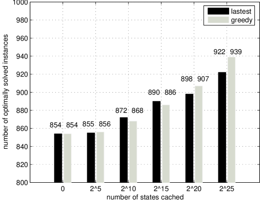
Figure 2: The impact of different parameter settings on the number of optimally solved instances.

To further test the impacts of different parameter settings on the average number of subproblems generated, we selected five Type 2 instance groups, namely $40\times 18$, $46\times 16$, $52\times 14$, $58\times 12$ and $64\times 10$. All instances in these five groups can be optimally solved using our branch-and-bound algorithm within 10 minutes of running time. We pictorially show the results associated with some parameter settings in Figure 3. We can clearly observe that the average number of subproblems generated decreases as the number of cached states increases. This is in accordance with our intuition since more cache slots store more states, which helps prune more search nodes and therefore reduces the number of subproblems. This figure also reveals that the greedy caching strategy outperforms the latest caching strategy in terms of the average number of subproblems generated when $C=2^{20}$ or $C=2^{25}$, while the latest caching strategy generally generates fewer subproblems when $C$ is small, i.e., $C=2^{10}$ or $C=2^{15}$. As a result, we adopted the greedy caching strategy and $C=2^{25}$ in the final implementation of our branch-and-bound algorithm.

$$\begin{array}[]{cc}\leavevmode\resizebox{227.62204pt}{}{\includegraphics{fig2_25_eps.eps}}&\leavevmode\resizebox{227.62204pt}{}{\includegraphics{fig2_20_eps.eps}}\\ \mbox{(a) \ \ }&\mbox{(b) \ \ }\\ &\\ \leavevmode\resizebox{219.08612pt}{}{\includegraphics{fig2_15_eps.eps}}&\leavevmode\resizebox{219.08612pt}{}{\includegraphics{fig2_10_eps.eps}}\\ \mbox{(c) \ \ }&\mbox{(d) \ \ }\end{array}$$

Figure 3: (a) $C=2^{10}$. (b) $C=2^{15}$. (c) $C=2^{20}$. (d) $C=2^{25}$.

5 Conclusions

In this paper, we proposed an enhanced branch-and-bound algorithm to solve the talent scheduling problem, which is a very challenging combinatorial optimization problem. This algorithm uses a new lower bound and two new dominance rules to prune the search nodes. In addition, it caches search states for the purpose of eliminating search nodes. The experimental results clearly show that our algorithm outperforms the current best approach and achieved the optimal solutions for considerably more benchmark instances.

We present a mixed integer linear programming model for the talent scheduling problem in Section 2. A possible future research direction is to design mathematical programming algorithms for the talent scheduling problem, such as branch-and-cut algorithm and branch-and-bound coupled with lagrangian relaxation and sub-gradient methods.

References

- Adelson et al. (1976) Adelson, R. M., Norman, J. M., Laporte, G., 1976. A dynamic programming formulation with diverse applications. Operational Research Quarterly, 119 – 121.
- Bomsdorf and Derigs (2008) Bomsdorf, F., Derigs, U., 2008. A model, heuristic procedure and decision support system for solving the movie shoot scheduling problem. Or Spectrum 30 (4), 751 – 772.
- Braune et al. (2012) Braune, R., Zäpfel, G., Affenzeller, M., 2012. An exact approach for single machine subproblems in shifting bottleneck procedures for job shops with total weighted tardiness objective. European Journal of Operational Research 218 (1), 76 – 85.
- Cheng et al. (1993) Cheng, T. C. E., Diamond, J. E., Lin, B. M. T., 1993. Optimal scheduling in film production to minimize talent hold cost. Journal of Optimization Theory and Applications 79 (3), 479 – 492.
- de la Banda et al. (2011) de la Banda, M. G., Stuckey, P. J., Chu, G., 2011. Solving talent scheduling with dynamic programming. INFORMS Journal on Computing 23 (1), 120 – 137.
- Drake and Hougardy (2003) Drake, D. E., Hougardy, S., 2003. A simple approximation algorithm for the weighted matching problem. Information Processing Letters 85 (4), 211 – 213.
- Dumas et al. (1995) Dumas, Y., Desrosiers, J., Gelinas, E., Solomon, M. M., 1995. An optimal algorithm for the traveling salesman problem with time windows. Operations research 43 (2), 367 – 371.
- Fink and Voß (1999) Fink, A., Voß, S., 1999. Applications of modern heuristic search methods to pattern sequencing problems. Computers and Operations Research 26 (1), 17 – 34.
- Hilden (1976) Hilden, J., 1976. Elimination of recursive calls using a small table of “randomly” selected function values. BIT Numerical Mathematics 16 (1), 60 – 73.
- Karp (1972) Karp, R. M., 1972. Reducibility among combinatorial problems. Springer.
- Kellegöz and Toklu (2012) Kellegöz, T., Toklu, B., 2012. An efficient branch and bound algorithm for assembly line balancing problems with parallel multi-manned workstations. Computers & Operations Research 39 (12), 3344 – 3360.
- Michie (1968) Michie, D., 1968. “memo” functions and machine learning. Nature 218 (5136), 19 – 22.
- Mingozzi et al. (1997) Mingozzi, A., Bianco, L., Ricciardelli, S., 1997. Dynamic programming strategies for the traveling salesman problem with time window and precedence constraints. Operations Research 45 (3), 365 – 377.
- Nordström and Tufekci (1994) Nordström, A.-L., Tufekci, S., 1994. A genetic algorithm for the talent scheduling problem. Computers & Operations Research 21 (8), 927 – 940.
- Pugh (1988) Pugh, W., 1988. An improved replacement strategy for function caching. In: Proceedings of the 1988 ACM conference on LISP and functional programming. ACM, pp. 269 – 276.
- Ranjbar et al. (2012) Ranjbar, M., Davari, M., Leus, R., 2012. Two branch-and-bound algorithms for the robust parallel machine scheduling problem. Computers & Operations Research 39 (7), 1652 – 1660.
- Rong and Figueira (2013) Rong, A., Figueira, J. R., 2013. A reduction dynamic programming algorithm for the bi-objective integer knapsack problem. European Journal of Operational Research 231 (2), 299 – 313.
- Smith (2003) Smith, B. M., 2003. Constraint programming in practice: Scheduling a rehearsal. Re-search Report APES-67-2003, APES group.
- Smith (2005) Smith, B. M., 2005. Caching search states in permutation problems. Lecture Notes in Computer Science 3709, 637 – 651.
- Zhang et al. (2012) Zhang, Z., Qin, H., Zhu, W., Lim, A., 2012. The single vehicle routing problem with toll-by-weight scheme: A branch-and-bound approach. European Journal of Operational Research 220 (2), 295 – 304.