Tidal evolution of the spin-orbit angle in exoplanetary systems

Abstract

The angle between the stellar spin and the planetary orbit axes (spin-orbit angle) is supposed to carry valuable information on the initial condition of the planet formation and the subsequent migration history. Indeed current observations of the Rossiter-McLaughlin effect have revealed a wide range of spin-orbit misalignments for transiting exoplanets. We examine in detail the tidal evolution of a simple system comprising a Sun-like star and a hot Jupiter adopting the equilibrium tide and the inertial wave dissipation effects simultaneously. We find that the combined tidal model works as a very efficient realignment mechanism; it predicts three distinct states of the spin-orbit angle (i.e., parallel, polar, and anti-parallel orbits) for a while, but the latter two states eventually approach the parallel spin-orbit configuration. The intermediate spin-orbit angles as measured in recent observations are difficult to be achieved. Therefore the current model cannot reproduce the observed broad distribution of the spin-orbit angles, at least in its simple form. This indicates that the observed diversity of the spin-orbit angles may emerge from more complicated interactions with outer planets and/or may be the consequence of the primordial misalignment between the proto-planetary disk and the stellar spin, which requires future detailed studies.

1 Introduction

More than 1000 exoplanets discovered so far have exhibited a surprising diversity in their physical properties. These are important observational clues to unveil their formation and evolution processes. In particular, unexpectedly large fractions of hot Jupiters (giant gaseous planets orbiting the central star with periods less than 1 week) and planets with highly eccentric and/or misaligned (their orbital axis is not aligned with the spin axis of the central star) orbits are regarded as serious challenges to conventional models of planet formation that have been proposed to explain the properties of our solar system. According to the standard core-accretion scenario, such gas giants are supposed to form beyond the ice line in nearly circular orbits. Thus it is widely believed that the discovered hot Jupiters should have formed at a large distance beyond the ice line, and then somehow migrated towards the orbits close to the central star (e.g., Ida & Lin, 2004a, b).

A widely accepted scenario is Type II migration in which gas giants migrate inward by the planet-disk interaction and halt at the inner edge of the disk (e.g., Lin et al., 1996). Other scenarios require dynamical processes after the depletion of the gas disk, including planet-planet scattering (e.g., Rasio & Ford, 1996; Nagasawa et al., 2008; Nagasawa & Ida, 2011), secular evolution (Wu & Lithwick, 2011), and the Kozai mechanism (Kozai, 1962; Wu & Murray, 2003; Fabrycky & Tremaine, 2007; Naoz et al., 2012). While the former normally predicts alignment of the stellar spin axis and the planetary orbital axis, the latter dynamical processes are found to enhance the eccentricity and inclination of planets. Thus, the spin-orbit angle distribution may be a useful discriminator of the planetary migration scenarios.

The projected angle ($\lambda$) between the stellar spin and the planetary orbit of transiting planets can be determined through the Rossiter-McLaughlin (RM) effect (Rossiter, 1924; McLaughlin, 1924; Queloz et al., 2000; Ohta et al., 2005; Winn et al., 2005; Hirano et al., 2011). The spin-orbit angle distribution may be a useful discriminator of the planetary migration scenarios. Indeed the RM effect has been measured successfully for around 70 transiting exoplanets as illustrated in Figure 7 below. Among them, 31 systems exhibit significant misalignment($\lambda>\pi/8$), including 12 polar- and 7 retrograde-orbits (see also Addison, 2013). These unexpected and counter-intuitive discoveries imply that close-in giant planets should have experienced violent dynamical processes, for instance, planet-planet scattering.

There is also a possibility that the spin-orbit misalignment may be imprinted even at the initial condition of the proto-planetary disk (e.g., Lai, Foucart & Lin, 2011; Batygin, 2013), but a reliable estimate of the distribution function of the initial spin-orbit angles is challenging. Thus, in this paper, we focus on the dynamical process among the star and planet in the later stage of planet formation.

If the dynamical process is the major path to form hot Jupiters, one may expect that the spin-orbit angle distribution just after the formation of hot Jupiters should be very broad, and even close to random. In order to be consistent with the observed distribution with some overabundance around alignment configuration, a fairly efficient physical process of the spin-orbit (re)alignment is required. While the subsequent tidal interaction between the central star and the innermost planet is generally believed to be responsible for the alignment, its detailed model is still unknown.

A conventional equilibrium tide model could realign the system, but inevitably accompanies the orbital decay of the planet within a similar timescale (Barker & Ogilvie, 2009; Levrard et al., 2009; Matsumura et al., 2010); see equation (4) below. Therefore a simple equilibrium tide model does not explain the majority of the realigned systems with finite semi-major axes.

In order to solve this problem, Winn et al. (2010) proposed a decoupling model in which the stellar convective envelope is weakly coupled to its radiative core, thus preferentially reducing the realignment timescale of the stellar envelope relative to that of the orbital decay. In reality, however, it is not clear to what extent the decoupling model can explain the observed distribution since there is no systematic and quantitative study of this model. In addition, the Sun is known to have a strong coupling between the convective and radiative zones (e.g., Howe, 2009), and theoretical support for this model seems weak.

Recently, Lai (2012) proposed a new model in which the damping timescale of the spin-orbit angle could be significantly smaller than that of the planetary orbit. When the stellar spin is misaligned with respect to the planetary orbital axis, one component in the tidal potential may excite inertial waves in the convective zone and provide a dynamical tidal response (e.g., Goodman & Lackner, 2009). This effect increases the efficiency of the realignment process without contributing to the orbital decay.

The model was studied in detail by Rogers & Lin (2013), who numerically integrated a set of simplified equations for the semi-major axis $a$, the spin angular frequency $\Omega_{\rm s}$, and the spin-orbit angle $\Theta$, originally derived by Lai (2012). They found that planetary systems with initially arbitrary spin-orbit angles have three stable configurations; parallel, anti-parallel, and polar orbits.

In the present paper, we use a full set of equations to trace the three-dimensional orbit of a planet (we assume that this represents the innermost planet in the case of multi-planetary systems) and the spin vector of the central star simultaneously, and examine the tidal evolution of exoplanetary systems on a longer time-scale. As a result, we find that both anti-parallel and polar orbits eventually approach the parallel orbit. We present a detailed comparison with the previous results by Rogers & Lin (2013), and argue that the full set of equations is important in understanding the longer-term evolution of the tidal model.

We briefly review the two tidal models, the equilibrium tide and the inertial wave dissipation, in §2, and describe how to combine the two models in our treatment. The basic set of equations is summarized explicitly in Appendix A. After comparing with the previous result in §3.1, we present the evolution in the combined tidal model in §3.2. We also consider there the dependence on the fairly uncertain parameters of the model. Section 4 is devoted to summary and discusses implications of the present result.

2 Tidal evolution of star–hot Jupiter systems

The entire dynamical evolution of planetary systems has many unresolved aspects including the initial structure of proto-planetary disks, formation processes of proto-planets, planetary migration, planet-planet gravitational scattering, and the tidal interaction between the central star and orbiting planets. It is definitely beyond the scope of the present paper to consider such complicated processes in a self-consistent fashion. Thus we consider a very simple system comprising a star and a hot Jupiter, and focus on their tidal interaction in order to examine the dynamical behavior of the stellar spin and the planetary orbit. Just for definiteness, we fix the mass and radius of the star and the planet as $m_{\rm s}=1M_{\odot}$, $m_{\rm p}=10^{-3}M_{\odot}$, and $R_{\rm s}=1R_{\odot}$. The initial semi-major axis of the planetary orbit is set as $a_{\rm ini}=0.02$AU.

We do not assume any specific formation mechanism, but the above configuration is expected generically from any successful models for hot Jupiter formation. The eccentricity and inclination of the hot Jupiter would depend on the details of the formation mechanism. The present study, however, focuses on the tidal evolution between the star and the hot Jupiter after the orbit circularization. Then we set the eccentricity of the planet to zero, and consider a wide range of the initial inclination of its orbit with respect to the spin axis of the star.

We numerically solve a set of equations (Correia et al., 2011) for the stellar spin angular momentum $\mathbf{S}=I_{\rm s}{\mathbf{\Omega}}_{\rm s}$ ($I_{\rm s}$ is the inertia moment of the star and ${\mathbf{\Omega}}_{\rm s}$ is the spin angular frenquency), and the orbital angular momentum $\mathbf{L}=m_{\rm p}m_{\rm s}/(m_{\rm p}+m_{\rm s})a^{2}{\mathbf{\Omega}}_{\rm p}$ (${\mathbf{\Omega}}_{\rm p}$ is the orbital mean motion) in order to explore the tidal evolution of the system. Correia et al. (2011) derived those equations for the equilibrium tide model (ET model, hereafter), which is based on the weak-friction model with a constant delay time $\Delta{t_{\rm L}}$ (Mignard, 1979).

We summarize the full equations in Appendix A that directly trace the three dimensional orbit of planets. If one neglects the eccentricity, the general relativity effect, and the tidal deformation of the planet, however, they lead to the following simplified equations for the semi-major axis $a$, the spin angular frequency $\Omega_{\rm s}$, and the spin-orbit angle $\Theta$ in the ET model (Lai, 2012):

$$\frac{(\dot{a})_{\rm e}}{a} = -\frac{1}{\tau_{\rm e}}\left(1-\frac{\Omega_{\rm s}}{\Omega_{\rm p}}\cos\Theta\right),$$ (1)

$$\frac{(\dot{\Omega}_{\rm s})_{\rm e}}{\Omega_{\rm s}} = \frac{1}{\tau_{\rm e}}\left(\frac{L}{2S}\right)\left[\cos\Theta-\frac{\Omega_{\rm s}}{2\Omega_{\rm p}}(1+\cos^{2}\Theta)\right],$$ (2)

$$(\dot{\Theta})_{\rm e} = -\frac{1}{\tau_{\rm e}}\left(\frac{L}{2S}\right)\sin\Theta\left[1-\frac{\Omega_{\rm s}}{2\Omega_{\rm p}}\left(\cos\Theta-\frac{S}{L}\right)\right].$$ (3)

The subscript e refers to the term due to the ET model.

As is clear from equations (1) to (3), $a$, $\Omega_{\rm s}$, and $\Theta$ have similar damping timescales characterized by

$$\tau_{\rm e} = \left(\frac{Q_{\rm e}}{3k_{2}}\right)\left(\frac{m_{\rm s}}{m_{\rm p}}\right)\left(\frac{a}{R_{\rm s}}\right)^{5}\Omega_{\rm p}^{-1}$$ (4)

$$\approx 1.3\left(\frac{Q_{\rm e}/3k_{2}}{2\times 10^{6}}\right)\left(\frac{m_{\rm s}}{10^{3}m_{\rm p}}\right)\left(\frac{\bar{\rho}_{\rm s}}{\bar{\rho}_{\odot}}\right)^{5/3}\left(\frac{P_{\rm p}}{1{\rm day}}\right)^{13/3}{\rm Gyr},$$ (5)

where $\bar{\rho}_{\rm s}$ is the mean density of the star, $P_{\rm p}$ is the orbital period of the planet, $Q_{\rm e}\equiv(2\Omega_{\rm p}\Delta t_{\rm L})^{-1}$ is the tidal quality factor of the star, and $k_{2}$ is the Love number of the star that represents gravity field deformation at the stellar surface in response to an external perturbing potential of spherical harmonic degree 2. We note that $k_{2}$ depends only on the internal density distribution of the star. The specific values of $\Delta{t_{\rm L}}$ and $k_{2}$ that we employ are shown in Table 1.

The fact that the ET model is basically governed by the single timescale is inconsistent with the presence of a number of well-aligned hot Jupiters orbiting at a finite distance from the star, as long as the ET model is the dominant mechanism for the spin-orbit (re)alignment. This is why Winn et al. (2010) proposed a decoupling model in which the star’s convective envelope is weakly coupled to its radiative core and $\Theta$ is damped efficiently without significant orbital decay of the planet.

Another model that we consider in detail below is proposed by Lai (2012), who pointed out the importance of the inertial waves of the star that are driven by the Coriolis force and dissipated by the tidal interaction of the misaligned $\mathbf{S}$ and $\mathbf{L}$. More specifically, he expanded the tidal potential due to the planet orbiting at $\mathbf{r}$ in the spherical coordinate system $(r,\theta,\phi)$ centered at the star with the $z$-axis along the stellar spin $\mathbf{S}$:

$$U_{2}(\mathbf{r},t)=-\sum_{m,m^{\prime}}U_{mm^{\prime}}(m_{\rm p},\Theta)r^{2}Y_{2m}(\theta,\phi)e^{-im^{\prime}\Omega_{\rm p}t},$$ (6)

where the index $m^{\prime}$ refers to that of spherical harmonics $Y_{2m^{\prime}}(\theta_{\rm L},\phi_{\rm L})$ defined in the coordinate with its $z$-axis along the planetary orbital angular momentum $\mathbf{L}$. Then he found that the only additional tidal torque in this model comes from $(m,m^{\prime})=(1,0)$ component.

The corresponding tidal torque components due to such dynamical tides are given in Lai (2012) as

$$T_{10,x} = \frac{3k_{10}}{4Q_{10}}T_{0}\sin{\Theta}\cos^{3}{\Theta},$$ (7)

$$T_{10,y} = -\frac{3k_{10}}{16}T_{0}\sin{4\Theta},$$ (8)

$$T_{10,z} = -\frac{3k_{10}}{4Q_{10}}T_{0}(\sin{\Theta}\cos{\Theta})^{2},$$ (9)

where $k_{10}$ and $Q_{10}$ are the dimensionless tidal Love number and tidal quality factor corresponding to the (1,0) component, and

$$T_{0}=G\left(\frac{m_{\rm p}}{a^{3}}\right)^{2}R_{\rm s}^{5}$$ (10)

(c.f., Murray & Dermott, 1999).

We note here that Lai (2012) chooses the $y$-direction along the direction ${\mathbf{S}}\times{\mathbf{L}}$. Thus $T_{10,y}$ does not change the spin-orbit elements, contributing to the spin precession, but we compute $T_{10,y}$ on the basis of equation (20) of Lai (2012) in any case. Up to the leading-order of the delay time, $T_{10,y}$ does not depend on $Q_{10}$ unlike $T_{10,x}$ nor $T_{10,z}$.

From the corresponding tidal torques due to the inertial wave dissipation described above, Lai (2012) derived the following equations for $a$, $\Omega_{\rm s}$, and $\Theta$:

$$(\dot{a})_{10} = 0,$$ (11)

$$\frac{(\dot{\Omega}_{\rm s})_{10}}{\Omega_{\rm s}} = -\frac{1}{\tau_{10}}\left(\sin\Theta\cos\Theta\right)^{2},$$ (12)

$$(\dot{\Theta})_{10} = -\frac{1}{\tau_{10}}\sin\Theta\cos^{2}\Theta\left(\cos\Theta+\frac{S}{L}\right).$$ (13)

In the above equations, $\tau_{10}$ is the characteristic tidal damping timescale corresponding to the (1,0) component:

$$\tau_{10} = \left(\frac{4Q_{10}}{3k_{10}}\right)\left(\frac{m_{\rm s}}{m_{\rm p}}\right)\left(\frac{a}{R_{\rm s}}\right)^{5}\left(\frac{S}{L}\right)\Omega_{\rm p}^{-1}$$ (14)

$$= 4\left(\frac{Q_{10}}{Q_{\rm e}}\right)\left(\frac{k_{2}}{k_{10}}\right)\left(\frac{S}{L}\right)\tau_{\rm e}.$$ (15)

Thus the inertial wave dissipation adds the damping terms with the timescale of $\tau_{10}$ for $\Theta$ and $\Omega_{s}$, while the planetary orbit is unaffected since the (1,0) component of the tidal potential is static in the inertial frame (Lai, 2012). Thus in this model the spin-orbit angle aligns faster before the planet falls into the central star, or more strictly, closer to its Roche limit $\approx 2R_{\rm s}(\bar{\rho}_{\rm s}/\bar{\rho}_{\rm p})^{1/3}$, if $\tau_{10}$ is much smaller than $\tau_{\rm e}$. The value of $\tau_{10}/\tau_{\rm e}$, however, is difficult to estimate in a reliable fashion. Thus we assume a fiducial value of $10^{-3}$ at the start of our simulation following Rogers & Lin (2013), and examine the dependence in §3.2.

We numerically integrate the set of equations shown in Appendix A for the ET model. For the Lai model, we modify the equations by adding the tidal torque $\mathbf{T}_{10}$ as

$$\dot{\mathbf{S}} = \dot{\mathbf{S}}_{\rm(e)}+{\mathbf{T}}_{10}-{\mathbf{T}}_{10,\rm e},$$ (16)

$$\dot{\mathbf{L}} = \dot{\mathbf{L}}_{\rm(e)}-{\mathbf{T}}_{10}+{\mathbf{T}}_{10,\rm e},$$ (17)

where the subscript (e) indicates the terms for the ET model, and ${\mathbf{T}}_{10,\rm e}$ is the term that is introduced to avoid the double counting in the above equations:

$$\frac{{\mathbf{T}}_{10,\rm e}}{{\mathbf{T}}_{10}} = \left(\frac{Q_{10}}{Q_{\rm e}}\right)\left(\frac{k_{2}}{k_{10}}\right).$$ (18)

Table 1 summarizes the fiducial values that we employ in the simulations. We use the same values for the stellar principal moment of inertia, the Love number and the tidal delay time that were adopted by Correia et al. (2011) for $\sim 1M_{\odot}$ star.

Parameter	symbol	Star	hot Jupiter
mass	$m[M_{\odot}]$	1	$10^{-3}$
radius	$R[R_{\odot}]$	1	—
principal moment of inertia	$C/mR^{2}$	0.08	—
Love number	$k_{2}$	0.028	—
tidal delay time	$\Delta{t_{\rm L}}[\rm sec]$	0.1	—

Table 1: Fiducial values of the parameters in our simulations.

3 Numerical results

3.1 Comparison with previous results

Before presenting a detailed analysis of the Lai model, we compare typical results arising from different tidal models and approximations. We consider two different tidal models: the ET model and the Lai model. Unlike in Rogers & Lin (2013), we refer to the Lai model which incorporates both the equilibrium tide and the inertial wave dissipation effects.

We numerically integrate the full set of equations in Appendix A throughout the paper. If one focuses on the evolution for $a$, $\Omega_{\rm s}$, and $\Theta$, the evolution equations in the Lai model can be reduced as follows:

$$\dot{a} = (\dot{a})_{\rm e},$$ (19)

$$\dot{\Omega}_{\rm s} = (\dot{\Omega}_{\rm s})_{\rm e}+(\dot{\Omega}_{\rm s})_{10}-(\dot{\Omega}_{\rm s})_{10,\rm e},$$ (20)

$$\dot{\Theta} = (\dot{\Theta})_{\rm e}+(\dot{\Theta})_{10}-(\dot{\Theta})_{10,\rm e},$$ (21)

where

$$\frac{(\dot{\Omega}_{\rm s})_{10,\rm e}}{(\dot{\Omega}_{\rm s})_{10}}=\frac{(\dot{\Theta})_{10,\rm e}}{(\dot{\Theta})_{10}}=\left(\frac{Q_{10}}{Q_{\rm e}}\right)\left(\frac{k_{2}}{k_{10}}\right).$$ (22)

In order to compare with the results from the full set of equations, we also integrate the above set of equations assuming the constant value for $(Q_{10}/Q_{\rm e})(k_{2}/k_{10})$. In practice, we use equation (14), and fix its value from the initial values of $\tau_{10}/\tau_{\rm e}$ and $S/L$:

$$\frac{Q_{10}}{Q_{\rm e}}\frac{k_{2}}{k_{10}}=\frac{1}{4}\left(\frac{\tau_{10}}{\tau_{\rm e}}\right)_{\rm ini}\left(\frac{S}{L}\right)^{-1}_{\rm ini}.$$ (23)

In the above simplified set of equations, $m_{\rm s}$ and $m_{\rm p}$ do not show up explicitly, but implicitly in $\tau_{10}$, $\tau_{\rm e}$, and $I_{\rm s}$. For definiteness, we fix $I_{s}=0.08m_{\rm s}R_{\rm s}^{2}$ (Wu & Murray, 2003; Correia et al., 2011). Thus $S/L$ and $\Omega_{\rm s}/\Omega_{\rm p}$ are related to each other as

$$\frac{\Omega_{\rm s}}{\Omega_{\rm p}}\approx 0.23\left(\frac{M_{\odot}}{m_{\rm s}}\right)\left(\frac{m_{\rm p}}{10^{-3}M_{\odot}}\right)\left(\frac{R_{\odot}}{R_{\rm s}}\right)^{2}\left(\frac{a}{0.02{\rm AU}}\right)^{2}\left(\frac{S}{L}\right).$$ (24)

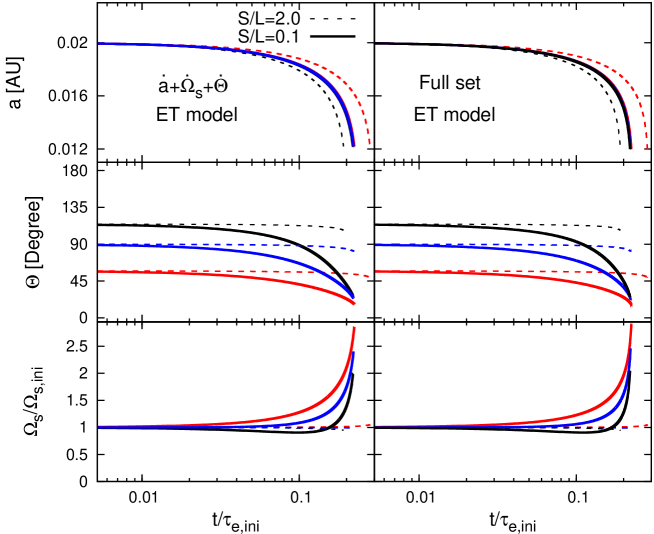
Figure 1: Evolution of the semi-major axis (Top), the spin-orbit angle (Center), and the spin angular frequency (Bottom) in the equilibrium tide model. Left and right panels are based on the numerical integration of the simplified and full sets of equations explained in the text. The three different initial spin-orbit angles are assumed; prograde ($\Theta_{\rm ini}=58^{\circ}$), polar ($\Theta_{\rm ini}=90^{\circ}$), and retrograde ($\Theta_{\rm ini}=116^{\circ}$) orbits, shown in red, blue, and black, respectively. The solid and dashed lines indicate the $(S/L)_{\rm ini}=0.1$ (solid) and $2$ (dashed).

Figure 1 shows evolution of $a$ (Upper panels), $\Theta$ (Center), and $\Omega_{\rm s}/\Omega_{\rm s,ini}$ (Lower) for the ET model. Left and right panels plot the results on the basis of the simplified set of equations for $a$, $\Omega_{\rm s}$ and $\Theta$ (eqs.(1) – (3)) and the full equations in Appendix A, respectively. Note that $\tau_{\rm e}$ completely specifies the units of time in the simulations. Thus the time evolution is scaled with respect to the initial value of $\tau_{\rm e}$. This is why those panels are plotted against $t/\tau_{\rm e,ini}$.

In each panel, we start the models with three different initial spin-orbit angles; prograde ($\Theta_{\rm ini}=58^{\circ}$), polar ($\Theta_{\rm ini}=90^{\circ}$), and retrograde ($\Theta_{\rm ini}=116^{\circ}$). They are shown in red, blue, and black lines, respectively. For each initial condition, we plot two cases with the $(S/L)_{\rm ini}=0.1$ (solid) and $2$ (dashed) roughly corresponding to the upper and lower limits of $S/L$ for planets observed via the RM effect (Rogers & Lin, 2013). We note here that the system evolved towards $\Theta=0$ regardless of $\Theta_{\rm ini}$.

As pointed out earlier by several authors, the spin-orbit alignment occurs almost simultaneously with the planetary orbital decay. More strictly, equations (1) and (3) indicate that the damping time-scales of the orbit and the spin-orbit angle are given by $\tau_{\rm e}$ and $(S/L)\tau_{\rm e}$, respectively. This explains the dependence on $(S/L)_{\rm ini}$ in the plots; compare solid and dashed lines.

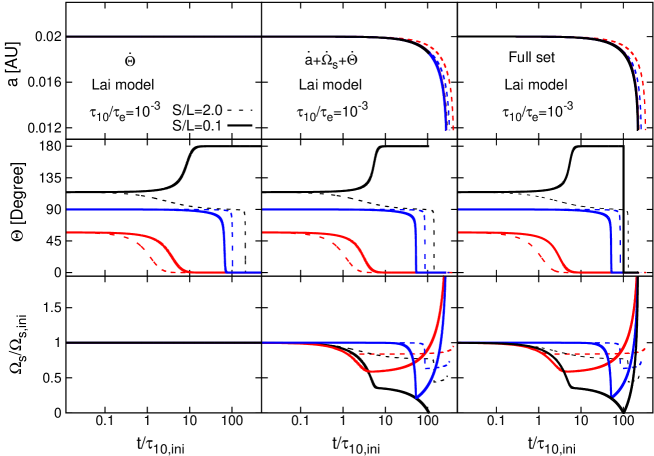
Figure 2: Same as Figure 1 but for the Lai model that combines the equilibrium tide and the inertial wave dissipation effects simultaneously. We add left panels that correspond to the result neglecting the change of $a$ and $\Omega_{\rm s}$.

The situation changes drastically in the Lai model, which introduces an additional time-scale $\tau_{10}$. Figure 2 shows an example of $(\tau_{10}/\tau_{\rm e})_{\rm ini}=10^{-3}$. In this case, the orbital decay proceeds according to the time-scale of $\tau_{\rm e}$, while the alignment time-scale is controlled by $\tau_{10}$ as well as $(S/L)\tau_{\rm e}$. Thus if $\tau_{10}\ll\tau_{\rm e}$, one can neglect the change of $a$ during the spin-orbit evolution. This is the approximation adopted by Rogers & Lin (2013), which corresponds to the left panels of Figure 2; we numerically integrate equation (21) neglecting the time evolution of $a$ and $\Omega_{s}$.

Rogers & Lin (2013) found that the system has three distinct stable configurations, i.e., anti-parallel ($\Theta=\pi$), polar ($\pi/2$), and parallel ($0$) orbits, which is easily expected from the right-hand-side of equation (21) as well. Nevertheless the damping on the order of $\tau_{\rm e}$ shows up in the later stage, and the polar orbit evolves towards $\Theta=0$. This can be hardly recognized in Figure 2 of Rogers & Lin (2013) because we suspect they stop the integration at $t=100\tau_{10}=0.1\tau_{\rm e}$, before their approximation $\dot{a}=0$ becomes invalid.

In reality, the evolution beyond the epoch should be computed taking account of the change of $a$ and $\Omega_{\rm s}$ properly. The middle panels show the result, and confirm that the polar orbit is a metastable configuration. Since the right-hand-sides of both equations (3) and (21) are proportional to $\sin\Theta$, the system should evolve eventually towards either $\Theta=0$ or $\pi$, but not $\pi/2$.

We found that the $\Theta=\pi$ configuration finally approaches $\Theta=0$ by integrating the full set of equations for the three dimensional planetary orbit. In the anti-parallel case, the spin-orbit angle has a sharp change between $\pi$ and $0$. This is because as the orbit damps, the stellar spin $S$ continuously decreases according to the total angular momentum conservation. At some point, therefore, the stellar spin becomes 0, changes the direction, and then starts to increase (aligned to the orbital axis). Thus the really stable configuration is $\Theta=0$ alone. Nevertheless the duration of such meta-stable configurations is also sensitive to the choice of $\tau_{10}/\tau_{\rm e}$ and/or $(S/L)_{\rm ini}$; see Figure 4. Thus the retro-grade and polar-orbit systems can be observed in the real systems depending on their age.

This behavior cannot be traced properly by the simplified approach, which is based on the differential equation for $\Theta$, combining equations (3) and (13); the right-hand-side of equations (3) diverges at $S=0$ or $\Omega_{s}=0$, and cannot be numerically integrated beyond the point. In contrast, the full set of equations in Appendix A computes ${\mathbf{S}}$ and ${\mathbf{L}}$ first, and $\Theta$ later. Thus one can compute the evolution continuously beyond ${\mathbf{S}}=0$. This is one of the advantages of using the full set of equations even in the case of the simple star-planet system.

In any case, we confirm the original claim of Lai (2012) that one can have an aligned system with a finite semi-major axis as long as $\tau_{10}/\tau_{\rm e}\ll 1$ is satisfied.

3.2 Spin-orbit angle evolution in the Lai model

Now we examine the Lai model more systematically using the full set of equations. We run 30 models of a planet with a regularly spaced $\Theta_{\rm ini}$ between $0^{\circ}$ and $180^{\circ}$. We plot the results in Figure 3 for $(S/L)_{\rm ini}=2$ (left), $0.5$ (middle), and $0.1$ (right). All the simulations adopt $(\tau_{10}/\tau_{\rm e})_{\rm ini}=10^{-3}$ so as to compare the middle panels of Figure 2 of Rogers & Lin (2013).

As explained in §3.1, the system first approaches parallel, polar, or anti-parallel orbits within a time-scale of $\tau_{10}$. They are plotted in black, blue, and red, respectively, so that they are easily distinguished visually. Next the polar, and subsequently anti-parallel orbits, approach towards the parallel orbits in a time-scale of $\tau_{\rm e}$, eventually falling below the Roche limit of the star (0.012 AU in the present case), where we stop the simulations.

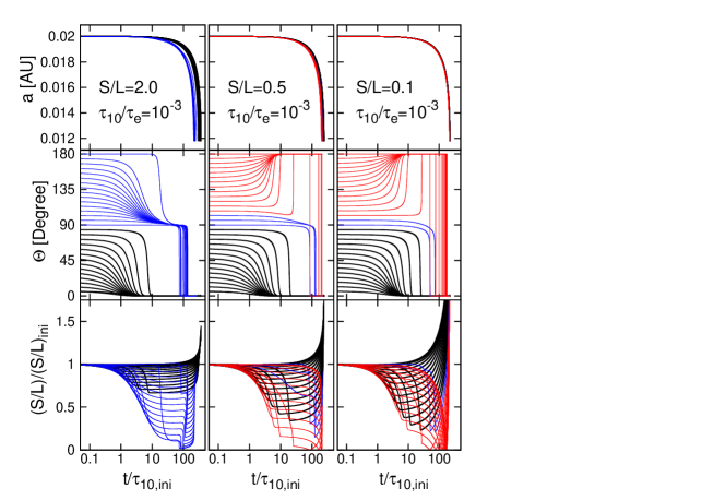
Figure 3: Evolution of the semi-major axis (Top), the spin-orbit angle (Middle), and $S/L$ (Bottom) in the Lai model for 30 systems with $\Theta_{\rm ini}$ from $0^{\circ}$ to $180^{\circ}$ with interval $6^{\circ}$. Left, center, and right panels indicate $(S/L)_{\rm ini}=2$, $0.5$, and $0.1$, respectively. The $(\tau_{10}/\tau_{\rm e})_{\rm ini}=10^{-3}$ is assumed. Blue and red lines indicate the systems that show the transition from polar to parallel, anti-parallel to parallel states, respectively.

The transition from $\Theta=180^{\circ}$ to $0^{\circ}$ (red curves) happens through a state of $\Omega_{\rm s}=0$, implying that the stellar spin starts counter-rotating due to the tidal effect of the orbiting planet. As mentioned in §3.1, the evolution beyond $\Omega_{\rm s}=0$ is difficult to trace with the simplified set of equations. Thus our simulations on the basis of the full set of equations are essential. Note that the transition to the three meta-stable configurations is fairly rapid. Therefore if the age of the system is larger than $\tau_{10}$ and smaller than $\tau_{\rm e}$, one may expect basically three distinct spin-orbit angles, but their broad distribution as observed (c.f., Figure 7 below) is not likely to be explained even taking into account the projection effect;see Figure 3 of Rogers & Lin (2013).

While Figure 3 is the main result of the paper, it remains to consider the dependence on the initial ratios of $(\tau_{10}/\tau_{\rm e})_{\rm ini}$, and $(\Omega_{\rm s}/\Omega_{\rm p})_{\rm ini}$. As we will show below, the behavior presented in Figure 3 is indeed robust against the choice of those parameters.

Figure 4 shows results of initially prograde (Top), polar (Center), and retrograde (Bottom), orbits with $(S/L)_{\rm ini}=2.0$, $0.5$, and $0.1$ for $(\tau_{10}/\tau_{\rm e})_{\rm ini}=10^{-4}$ (black), $10^{-3}$ (blue), $10^{-2}$ (green), and $10^{-1}$ (red). The ratio $\tau_{10}/\tau_{\rm e}$ reflects the property of the stellar fluid itself, and thus is not easy to predict in a reliable fashion. Therefore we consider a fairly wide range of its possible value. The initially prograde cases approach $\Theta=0$ with a time-scale of $\tau_{10}$ fairly clearly. The initially polar-orbit cases stay the configuration for a significantly longer period than $\tau_{10}$, but eventually approach $\Theta=0$. The initially retrograde cases are somewhat intermediate between the two. In any case, the behavior changes systematically with the value of $(\tau_{10}/\tau_{\rm e})_{\rm ini}$ and can be interpolated/extrapolated relatively easily from Figure 4.

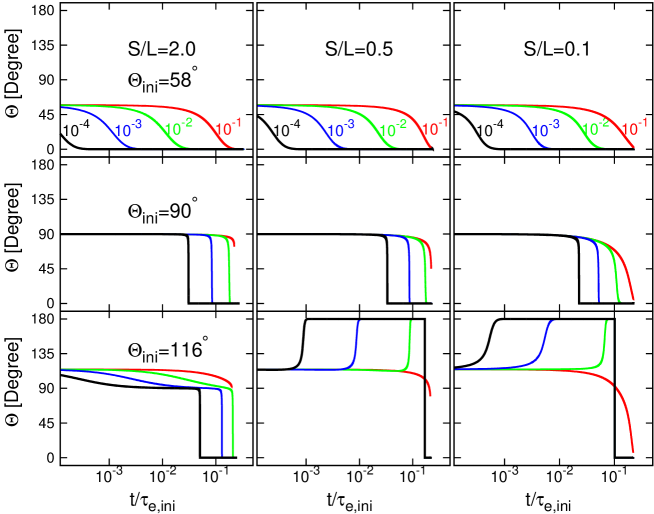
Figure 4: Dependence on the tidal dissipation parameter $(\tau_{10}/\tau_{\rm e})_{\rm ini}$ for $(S/L)_{\rm ini}=2.0$ (Left), $0.5$ (Middle), $0.1$ (Right). Black, Blue, Green, Red line represent $(\tau_{10}/\tau_{\rm e})_{\rm ini}=10^{-4},10^{-3},10^{-2},10^{-1}$; Top, center, and bottom panels indicate initially prograde, polar, and retrograde orbits, respectively.

Figure 5 shows the dependence on the planet mass $m_{\rm p}$, or equivalently on $(\Omega_{\rm s}/\Omega_{\rm p})_{\rm ini}$ through equation (24). Since our simulations adopt $m_{\rm s}=1M_{\odot}$, $R_{\rm s}=1R_{\odot}$, and $m_{\rm p}=10^{-3}M_{\odot}$, equation (24) determines the value of $\Omega_{\rm s}/\Omega_{\rm p}$ uniquely through $(S/L)_{\rm ini}$. In contrast, Rogers & Lin (2013) vary the value randomly in the range of $0.1<(\Omega_{\rm s}/\Omega_{\rm p})_{\rm ini}<10$, while they do not describe exactly how. Equation (24) implies that the corresponding values of $(\Omega_{\rm s}/\Omega_{\rm p})_{\rm ini}$ in our model with $m_{\rm p}=10^{-3}M_{\odot}$ are $0.46$, $0.11$, and $0.02$ for $(S/L)_{\rm ini}=2$, $0.5$, and $0.1$, respectively. In order to see the dependence, we simply repeat the simulations with $m_{\rm p}=10^{-2}M_{\odot}$, keeping the other parameters exactly the same. Thus the $m_{\rm p}=10^{-2}M_{\odot}$ case corresponds to an order of magnitude increase of $(\Omega_{\rm s}/\Omega_{\rm p})_{\rm ini}$ relative to the $m_{\rm p}=10^{-3}M_{\odot}$ case. We do not run the case with $m_{\rm p}=10^{-2}M_{\odot}$ and $(S/L)_{\rm ini}=2$ since it does not satisfy the criterion $\Omega_{\rm p}\gg\Omega_{\rm s}$, under which the $(m,m^{\prime})=(1,0)$ is the only excitation mode (Lai, 2012). Figure 5 basically shows that the result depends on $(\Omega_{\rm s}/\Omega_{\rm p})_{\rm ini}$ very weakly.

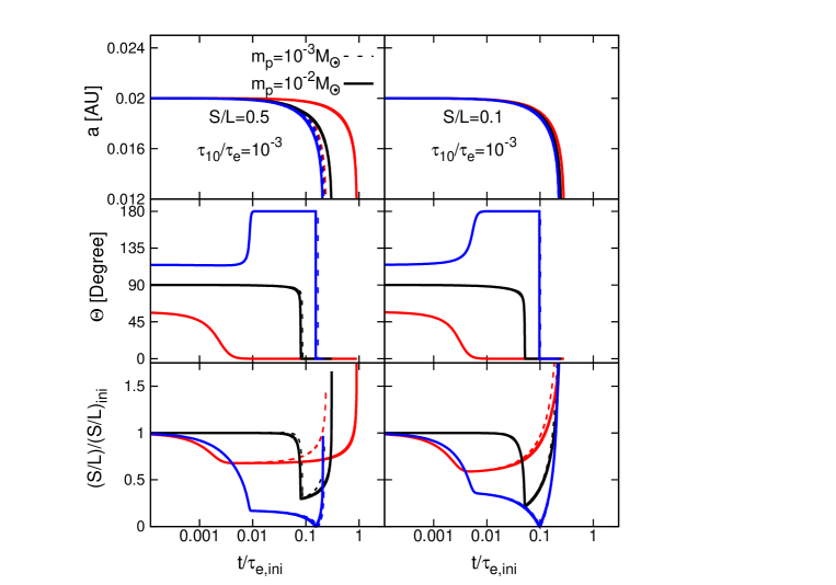
Figure 5: Dependence on the planet mass $m_{\rm p}$, or equivalently on $(\Omega_{\rm s}/\Omega_{\rm p})_{\rm ini}$, for $(S/L)_{\rm ini}=0.5$ (Left), $0.1$ (Right). The blue, black and red lines correspond to initial retrograde, polar and prograde orbit, while the solid and dashed lines to $m_{\rm p}=10^{-2}M_{\odot}$ and $10^{-3}M_{\odot}$, respectively.

4 Summary and discussion

We have considered tidal evolution of star–hot Jupiter systems with particular attention to their spin-orbit alignment. We focused on the inertial wave dissipation model proposed by Lai (2012), and examined the extent to which the model reproduces the observed distribution of spin-orbit angles for transiting exoplanets.

Basically we confirmed the conclusion of Rogers & Lin (2013) that the Lai model has three distinct stable configurations, anti-parallel, polar, and parallel orbits. In reality, however, the former two turn out to be meta-stable, and approach the parallel orbits over a longer time-scale as the equilibrium tide effect exceeds that of the inertial wave dissipation. We also found that the later evolution stage needs to be examined using direct three dimensional integrations for the spin vector and orbital angular momentum vector of the system, rather than the simplified differential equations for the semi-major axis, spin angular frequency, and spin-orbit angle, even when a simple star–planet system is considered.

The relative importance of the two tidal effects is determined by the ratio of $\tau_{\rm e}$ and $\tau_{10}$. Unfortunately there is a huge uncertainty in predicting the value of each parameter. Nevertheless in order to achieve a spin-orbit alignment at a finite planetary orbit, $\tau_{\rm 10}\ll\tau_{\rm e}$ is required. In such cases, however, the alignment due to the inertial wave dissipation works too efficiently, and the observed broad distribution of $\Theta$ for transiting planets (more precisely, the projected angle $\lambda$ of $\Theta$ onto the sky plane) is difficult to reproduce.

To illustrate this point, we simulate 50 systems with a planet located initially at 0.02AU and a randomly chosen $\Theta_{\rm ini}$ for $(S/L)_{\rm ini}=2$, $0.5$, and $0.1$. Figure 6 plots resulting $\Theta$ against $a$ at four different epochs; $t/\tau_{\rm e,ini}=0$, $0.03$, $0.07$, and $0.1$. While the ET model (Upper) predicts a relatively continuous correlation between $\Theta$ and $a$, the Lai model (Lower) has the distinct three (meta-)stable states, but they subsequently become completely aligned by $t=0.1\tau_{\rm e}$. The evolution is so rapid that even the different value of the initial semi-major axis cannot broaden the distribution significantly.

The observed distribution of the projected spin-orbit angles $\lambda$ is plotted in Figure 7 on the basis of the Holt-Rossiter-McLaughlin Encyclopedia compiled by René Heller; the radial coordinate of each symbol corresponds to the logarithm of the orbital period of the planet ($P\propto a^{3/2}$), and its angular coordinate represents the observed value of $\lambda$. Black and red circles indicate the innermost planets in single transiting systems, and the largest planets in the multi-transiting systems, respectively. The range of the solar-system planets is plotted in a blue region.

There is a clear tendency of clumping around $0<\lambda<30^{\circ}$, in addition to the dominance of the prograde orbits relative to the retrograde ones. Nevertheless the distribution is rather broad, and does not seem to be consistent with that expected from Figure 6. In order to make more quantitative comparison, one needs to consider the effect of projection since $\lambda$ is different from $\Theta$, but corresponds to its projected angle on the sky. The effect, however, does not change the main conclusion, and we will leave the detailed analysis to our future study.

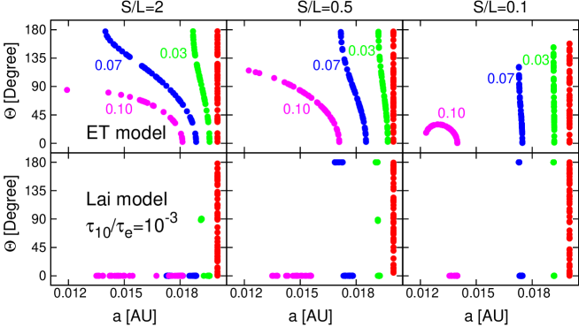
Figure 6: Spin-orbit angle plotted against the semi-major axis at different epochs; $t=0$ (red), $t=0.03\tau_{\rm e}$ (green), $t=0.07\tau_{\rm e}$ (blue), and $t=0.1\tau_{\rm e}$ (magenta). The upper and lower panels correspond to the equilibrium tide and Lai models, respectively, for 50 systems with randomly distributed $\Theta_{\rm ini}$. The initial values of $S/L$ are $2$ (Left), $0.5$ (Center), and $0.1$ (Right).

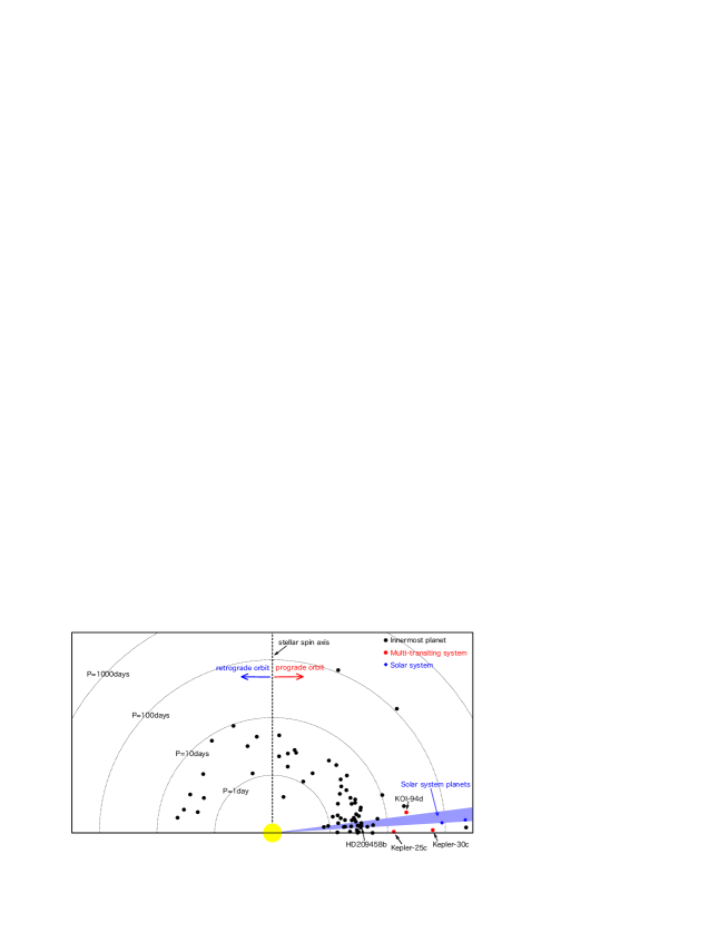
Figure 7: The projected misalignment angles $\lambda$ for transiting planets as of August 20, 2013. Black circles indicate innermost planets in single transiting systems, while red circles denote the largest planets in the three multi-transiting systems, Kepler-25c(Albrecht et al., 2013), Kepler-30c(Sanchis-Ojeda et al., 2012), and KOI-94d(Hirano et al., 2012; Masuda et al., 2013).

In this sense, we agree with the overall conclusion of Rogers & Lin (2013) that the Lai model, at least in the current simple star–planet system, cannot explain the wide range of observed $\lambda$. Furthermore, the current model is unlikely to explain the empirical trend that the realigned systems are preferentially found in the host stars with $T_{\rm eff}<6250$ K (Winn et al., 2010). Nevertheless we have to recognize that the planetary system considered in this paper is oversimplified; we ignore the outer planets that may influence the dynamics of the innermost planet significantly and the host-star dependence of the tidal parameters. In addition, we totally neglect the dependence on the initial conditions before the tidal realignment. Thus it is premature to make a negative conclusion, and we should explore the wider range of system configurations. For this purpose, the simplified set of equations is inappropriate, and we need to integrate three dimensional orbits of multi-planets using the full set of equations (Correia et al., 2011). Also it is important and interesting to examine three dimensional evolution of the spin and orbital angular momenta directly, instead of that of their mutual angle alone.

Appendix Appendix A Basic equations for tidal evolution

The present paper considers a hybrid tidal model which combines a conventional equilibrium tide model with the inertial tidal dissipation model proposed by Lai (2012). Just for completeness, we explicitly give a full set of basic equations that we numerically integrate. The equations are derived by Correia et al. (2011) for the equilibrium tide model for a system of a central star and two planets with arbitrary orbital eccentricities. The tidal interaction between the stellar spin and the planetary orbit is based on the weak-friction model with a constant delay time $\Delta{t}$ (Mignard 1979). Furthermore the general relativity correction and the stellar oblateness are taken into account.

In the present paper, we focus on the tidal interaction between the star and the innermost planet. Thus we neglect the distant planet for simplicity. The tide on the planet is not considered either because it should have a very negligible effect on the dynamics of the star and planet. Furthermore since we fix the initial eccentricity as 0 in the current simulations, the GR effect is also neglected.

Let us denote their mass by $m_{\rm s}$ and $m_{\rm p}$, the semi-major axis by $a$, the spin angular velocity by $\Omega_{\rm s}$, the orbital angular velocity by $\Omega_{\rm p}$, radius by $R_{\rm s}$ and gravity coefficient by $J_{2_{s}}$. The equations are written in terms of the Jacobi coordinates with $\mathbf{r}_{1}$ being the relative position from $m_{\rm s}$ to $m_{\rm p}$ under the quadrupole approximation for the conservative and tidal potentials of the system (e.g. Smart, 1953; Kaula, 1964; Correia et al., 2011).

The evolution of spin of star and orbit of planet can be specified in the quadrupole approximation by two parameters;

1) star rotational angular momentum:

$$\mathbf{S}=C_{\rm s}\Omega_{\rm s}\hat{\mathbf{s}},$$ (A.1)

where $\hat{\mathbf{s}}$ is the unit vector of $\hat{\mathbf{S}}$, and $C_{\rm s}$ is the principal moment of inertia.

2)orbital angular momentum:

$$\mathbf{L}=\beta\sqrt{{\mu}a}\hat{\mathbf{k}},$$ (A.2)

where $\hat{\mathbf{k}}$ is the unit vector of $\hat{\mathbf{L}}$, $\mu=G(m_{\rm s}+m_{\rm p})$, and $\beta=m_{\rm s}m_{\rm p}/(m_{\rm s}+m_{\rm p}$).

We define $\Theta$, the angle between the spin of the star and the orbit of the innermost planet via

$$\cos\Theta=\hat{\mathbf{s}}\cdot\hat{\mathbf{k}}.$$ (A.3)

As Correia et al. (2011) described in detail, the evolution of the system is governed by the conservative motion and the tidal effects. First, the equation for conservative motion is obtained by averaging the equations of motion over the mean anomaly:

$$\dot{\mathbf{L}}_{(\rm c)} = \alpha\cos\Theta\hat{\mathbf{s}}\times\hat{\mathbf{k}},$$ (A.4)

$$\dot{\mathbf{S}}_{(\rm c)} = -\alpha\cos\Theta\hat{\mathbf{s}}\times\hat{\mathbf{k}},$$ (A.5)

where $L$ is the norm of $\mathbf{L}$, and

$$\alpha = \frac{3Gm_{\rm s}m_{\rm p}J_{2_{s}}R_{s}^{2}}{2a^{3}}.$$ (A.6)

Second, the equilibrium tidal effect is considered under the quadrupole approximation of the tidal potential assuming the constant delay time $\Delta{t_{\rm L}}$ (Mignard, 1979). After averaging equations of motion over the mean anomaly, one obtains

$$\dot{\mathbf{L}}_{(\rm t)} = -\dot{\mathbf{S}}_{(\rm t)},$$ (A.7)

$$\dot{\mathbf{S}}_{(\rm t)} = K\Big{[}\frac{\Omega_{\rm s}}{2}(\hat{\mathbf{s}}-\cos\Theta\hat{\mathbf{k}})-\Omega_{\rm s}\hat{\mathbf{s}}+\Omega_{\rm p}\hat{\mathbf{k}}\Big{]},$$ (A.8)

where

$$K = \Delta{t_{\rm L}}\frac{3k_{2}Gm_{\rm p}^{2}R_{\rm s}^{5}}{a^{6}},$$ (A.9)

Thus the total rates of change of $L$ and $S$ under the equilibrium tidal model are given by the sum of the above terms corresponding to the conservative motion and tidal effect:

$$\dot{\mathbf{L}}_{(\rm e)} = \dot{\mathbf{L}}_{(\rm c)}+\dot{\mathbf{L}}_{(\rm t)},$$ (A.10)

$$\dot{\mathbf{S}}_{(\rm e)} = \dot{\mathbf{S}}_{(\rm c)}+\dot{\mathbf{S}}_{(\rm t)}.$$ (A.11)

Finally, we add the tidal torque due to the inertial wave dissipation, equations (7) to (9) to the above equations as in equations (16) and (17).

References

- Addison (2013) Addison, B. C., Tinney, C. G., Wright, D. J., Bayliss, D., Zhou, G., Hartman, J. D., Bakos, G. A., & Schmidt, B. 2013, ApJ, 774, L9
- Albrecht et al. (2013) Albrecht, S., Winn, J.N., Marcy, G.W., Howard, A.W., Isaacson, H., & Johnson, J.A. 2013, ApJ, 771, 11
- Barker & Ogilvie (2009) Barker, A. J., & Ogilvie, G. I. 2009, MNRAS, 395, 2268
- Batygin (2013) Batygin, K. 2013, Nature, 491, 418-420
- Beauge & Nesvorny (2012) Beauge C., & Nesvorny D., 2012, AJ 751, 119
- Correia et al. (2011) Correia, A. C. M., Laskar, J., Farago, F., & Boue, G. 2011, Celest. Mech. Dyn. Astron., 111, 105
- Fabrycky & Tremaine (2007) Fabrycky,D. & Tremaine, S. 2007, ApJ, 669, 1298
- Goodman & Lackner (2009) Goodman, J. & Lackner, C. 2009, ApJ, 696, 2054
- Hirano et al. (2011) Hirano, T., Suto, Y., Winn, J. N., Taruya, A., Narita, N., Albrecht, S., & Sato, B. 2011, ApJ, 742, 69
- Hirano et al. (2012) Hirano, T., Narita, N., Sato, B., Takahashi, Y.H., Masuda, K., Takeda, Y., Aoki, W., Tamura, M. & Suto, Y. 2012, ApJ, 759, L36
- Howe (2009) Howe, R. 2009, Living Rev. Sol. Phys., 6, 1
- Ida & Lin (2004a) Ida, S., & Lin, D. N. C. 2004, ApJ, 604, 388
- Ida & Lin (2004b) Ida, S., & Lin, D. N. C. 2004, ApJ, 616, 567
- Kaula (1964) Kaula,W.M. 1964, Rev.Geophys., 2, 661
- Kozai (1962) Kozai, Y. 1962, AJ, 67, 591
- Lai, Foucart & Lin (2011) Lai D., Foucart F., Lin D. N. C., 2011, MNRAS, 412, 2790
- Lai (2012) Lai, D. 2012, MNRAS, 423, 486
- Levrard et al. (2009) Levrard B., Winisdoerffer C., & Chabrier G., 2009, ApJ, 692, L9
- Lin et al. (1996) Lin, D. N. C., Bodenheimer, P., & Richardson, D. 1996, Nature, 380, 606
- Masuda et al. (2013) Masuda,K., Hirano,T., Taruya,A., Nagasawa,M., & Suto, Y. 2013, ApJ, 778, 185
- Matsumura et al. (2010) Matsumura S., Peale S. J., & Rasio F. A., 2010, ApJ, 725, 1995
- McLaughlin (1924) McLaughlin, D. B. 1924, ApJ, 60, 22
- Mignard (1979) Mignard, F., Moon Planets 1979, 20, 301-315
- Murray & Dermott (1999) Murray, C.D., & Dermott, S.F. 1999, Solar System Dynamics (Cambridge Univ. Press; Cambridge, New York)
- Nagasawa et al. (2008) Nagasawa, M., Ida, S., & Bessho, T. 2008, ApJ, 678, 498
- Nagasawa & Ida (2011) Nagasawa, M., & Ida, S. 2011, ApJ, 742, 72
- Naoz et al. (2011) Naoz, S., Farr, W. M., Lithwick, Y., Rasio, F. A., & Teyssandier, J. 2011, Nature, 473, 187
- Naoz et al. (2012) Naoz, S., Farr, W. M., & Rasio, F.A., ApJ, 2012, 754, L36
- Ohta et al. (2005) Ohta, Y., Taruya, A., & Suto Y. 2005, ApJ, 622, 1118
- Queloz et al. (2000) Queloz, D., Eggenberger, A., Mayor, M., Perrier, C., Beuzit, J. L., Naef, D., Sivan, J. P., & Udry, S. 2000, A&A, 359, L13
- Rasio & Ford (1996) Rasio, F. & Ford, E. 1996, Science, 274, 954
- Rogers & Lin (2013) Rogers, T.M. , & Lin, D.N.C. 2013, ApJL, 769:L10
- Rossiter (1924) Rossiter, R. A. 1924, ApJ, 60, 15
- Sanchis-Ojeda et al. (2012) Sanchis-Ojeda, R., Fabrycky, D. C., Winn, J. N., et al. 2012, Nature, 487, 449
- Smart (1953) Smart, W.M. 1953, Celestial Mechanics (Longmans; London, New York)
- Triaud (2011) Triaud A., 2011, A&A, 534, L6
- Winn et al. (2005) Winn, J. N., Noyes, R.W., Holman, M.J., Charbonneau, D., Ohta, Y., Taruya, A., Suto, Y., Narita, N., Turner, E.L., Johnson, J.A., Marcy, G.W., Butler, R.P., & Vogt, S.S. 2005, ApJ, 631, 1215
- Winn et al. (2010) Winn J. N., Fabrycky D., Albrecht S., & Johnson J. A., 2010, ApJ, 718, L145
- Wu & Lithwick (2011) Wu, Y., & Lithwick, Y. 2011, ApJ, 735, 109
- Wu & Murray (2003) Wu, Y., & Murray, N. 2003, ApJ, 589, 605