A Generalization of Threshold Saturation: Application to Spatially Coupled BICM-ID

Abstract

Spatial coupling was proved to improve the belief-propagation (BP) performance up to the maximum-a-posteriori (MAP) performance. This paper addresses an extended class of spatially coupled (SC) systems. A potential function is derived for characterizing a lower bound on the BP performance of the extended SC systems, and shown to be different from the potential for the conventional SC systems. This may imply that the BP performance for the extended SC systems does not coincide with the MAP performance for the corresponding uncoupled system. SC bit-interleaved coded modulation with iterative decoding (BICM-ID) is also investigated as an application of the extended SC systems.

I Introduction

Kudekar et al. [1] proved that spatial coupling can improve the belief-propagation (BP) threshold up to the maximum-a-posteriori (MAP) threshold. Since the original proof of this threshold saturation was complicated, several simpler proofs have been developed in [2, 3, 4, 5, 6]. In this paper we generalize the methodology in [4] to characterize the BP performance for extended spatially-coupled (SC) systems.

Consider the density-evolution (DE) equations of an extended SC system with the number of sections $L$ and coupling width $W$

$$u_{l}(i+1)=\frac{1}{W^{d}}\sum_{\boldsymbol{w}_{d}\in\mathcal{W}^{d}}\varphi(\boldsymbol{v}_{l+\boldsymbol{w}_{d}}(i)),\quad l\in\mathcal{L},$$ (1)

$$v_{l}(i)=\frac{1}{W^{\tilde{d}}}\sum_{\boldsymbol{w}_{\tilde{d}}\in\mathcal{W}^{\tilde{d}}}\psi(\boldsymbol{u}_{l-\boldsymbol{w}_{\tilde{d}}}(i)),\quad l\in\{W-1,\ldots,L-1\},$$ (2)

with $\mathcal{L}=\{0,\ldots,L-1\}$ and $\mathcal{W}=\{0,\ldots,W-1\}$. For notational convenience, we have used the notation $\boldsymbol{v}_{l+\boldsymbol{w}_{d}}(i)=(v_{l+w_{1}}(i),\ldots,v_{l+w_{d}}(i))$ and $\boldsymbol{u}_{l-\boldsymbol{w}_{\tilde{d}}}(i)=(u_{l-w_{1}}(i),\ldots,u_{l-w_{\tilde{d}}}(i))$, with $\boldsymbol{w}_{k}=(w_{1},\ldots,w_{k})$. The notation $l+\boldsymbol{w}$ should be interpreted as $(l,\ldots,l)+\boldsymbol{w}$. In (1) and (2), the state $(u_{l}(i),v_{l}(i))\in\mathcal{D}\times\tilde{\mathcal{D}}\subset\mathbb{R}^{2}$ represents performance of a BP-based algorithm for section $l\in\mathcal{L}$ in iteration $i$. The two functions $\varphi:\tilde{\mathcal{D}}^{d}\rightarrow\mathcal{D}$ and $\psi:\mathcal{D}^{\tilde{d}}\rightarrow\tilde{\mathcal{D}}$ characterize the properties of the BP algorithm. The parameters $d+1$ and $\tilde{d}+1$ correspond to the degrees of check and variable nodes in low-density parity-check (LDPC) codes. In bit-interleaved coded modulation, $d+1$ is equal to the modulation rate, whereas $\tilde{d}=1$ is used.

Without loss of generality, we postulate that larger variables $u_{l}(i)$ and $v_{l}(i)$ imply better performance. Let $(u_{\mathrm{opt}},v_{\mathrm{opt}})$ denote a fixed-point (FP) that has the largest $u$ among all FPs of the DE equations for the uncoupled case $W=1$. Thus, $(u_{\mathrm{opt}},v_{\mathrm{opt}})$ is a solution $(u,v)$ to the following FP equations:

$$u=\varphi_{0}(v),\quad v=\psi_{0}(u),$$ (3)

with $\varphi_{0}(v)=\varphi(v,\ldots,v)$ and $\psi_{0}(u)=\psi(u,\ldots,u)$. The FP $(u_{\mathrm{opt}},v_{\mathrm{opt}})$ corresponds to the best possible performance achieved by the BP algorithm.

We assume that $\varphi(v_{1},\ldots,v_{d})$ and $\psi(u_{1},\ldots,u_{\tilde{d}})$ are bounded, smooth, and strictly increasing in all arguments everywhere. The monotonicity implies that the performance of the BP algorithm improves monotonically. We impose the worst initial condition $u_{l}(0)=u_{\mathrm{min}}=\inf\mathcal{D}$ for all $l\in\mathcal{L}$ and the best boundary conditions $v_{l}(i)=v_{\mathrm{opt}}$ for any $l\notin\{W-1,\ldots,L-1\}$ and $i$. The aim of spatial coupling is to let the state $(u_{l}(i),v_{l}(i))$ converge toward $(u_{\mathrm{opt}},v_{\mathrm{opt}})$ for all sections $l\in\mathcal{L}$ after sufficiently many iterations via coupling.

We consider the continuum limit in which $L$ and $W$ tend to infinity while the ratio $\alpha=W/L$ is kept constant. The BP performance for the SC systems (1) and (2) is characterized by a potential function for the uncoupled system

$$V(u)= \int\left\{u-\varphi_{0}(\psi_{0}(u))\right\}\psi_{0}^{\prime}(u)$$ (4)

$$\cdot\exp\left\{D(u;\psi)+D(\psi_{0}(u);\varphi)\right\}du,$$

with

$$D(u;\psi)=\int\frac{\bigtriangleup\psi(u)}{\psi^{\prime}_{0}(u)}du-\ln\psi_{0}^{\prime}(u),$$ (5)

where the single-variate Laplacian $\bigtriangleup\psi(u)$ is given by $\bigtriangleup\psi(u)=\sum_{j}\partial^{2}\psi/\partial u_{j}^{2}(u,\ldots,u)$. The goal of this paper is to prove the following statement:

Theorem 1.

Take the continuum limit $W=\alpha L\to\infty$, the infinite-iteration limit $i\to\infty$, and finally the limit $\alpha\to 0$. If $u_{\mathrm{opt}}$ is the unique global stable solution (global minimizer) of the potential (4), the state $(u_{l}(i),v_{l}(i))$ convergences to the target solution $(u_{\mathrm{opt}},v_{\mathrm{opt}})$ in the limits above.

Theorem 1 is a generalization of previous works [2, 3, 6, 4, 5] for $d=\tilde{d}=1$, and implies that the qualitative shape of the potential (4) determines whether the BP algorithm can achieve the best possible performance point $(u_{\mathrm{opt}},v_{\mathrm{opt}})$, whereas the uniqueness of solutions to the potential (4) does for the uncoupled case $W=1$. The potential (4) reduces to the conventional one defined in [2] for $d=\tilde{d}=1$, and coincides with the conventional one for $d,\tilde{d}>1$ if $D(u;\psi)+D(\psi_{0}(u);\varphi)$ is independent of $u$. The latter observation may imply that for $d,\tilde{d}>1$ the BP threshold does not coincide with the MAP threshold for the corresponding uncoupled system, since the potential for $d=\tilde{d}=1$ is used to characterize the MAP threshold.

Theorem 1 is useful when no analytical formulas of the multi-variate functions $\varphi$ and $\psi$ in (1) and (2) are available. In this case, the cost for calculating the two functions numerically increases exponentially as $d$ and $\tilde{d}$ grow. Theorem 1 implies that we can know the BP performance just by estimating six single-variate functions $\varphi_{0}$, $\varphi_{0}^{\prime}$, $\bigtriangleup\varphi$, $\psi_{0}$, $\psi_{0}^{\prime}$, and $\bigtriangleup\psi$ via numerical integration or sampling.

This paper is organized as follows: In Section II we shall present an application of Theorem 1 to SC bit-interleaved coded modulation with iterative decoding (BICM-ID). Theorem 1 is proved in Section III.

II Application

II-A Spatially Coupled BICM-ID

We consider a BICM-ID scheme with SC interleaving [7]. One transmission consists of $W-1$ binary training sequences of length $M$ and of $L-(W-1)$ binary codewords of length $M$. The training sequences are utilized to anchor the performance of the system at the boundaries to the best performance $v_{\mathrm{opt}}$. After SC interleaving of length $LM$, the obtained binary sequences are mapped to $LM/Q$ data symbols, with $Q$ denoting the modulation rate. The data symbols are transmitted through a memoryless time-invariant communication channel, and detected with iterative decoding at the receiver side [8].

We shall review a construction of SC interleaving [7]. Let $\{\pi_{l}^{\mathrm{in}}:l\in\mathcal{L}\}$ and $\{\pi_{l}^{\mathrm{out}}:l\in\mathcal{L}\}$ denote $2L$ independent random interleavers of length $M$ that are bijections from $\mathcal{M}=\{0,\ldots,M-1\}$ onto $\mathcal{M}$. An SC interleaver $\pi(m,l)$ is a bijection from $\mathcal{M}\times\mathcal{L}$ onto $\mathcal{M}\times\mathcal{L}$ that maps $m$th bit in section $l$ to the pair $\pi(m,l)$ of bit and section indices,

$$\pi(m,l)=(\pi_{l^{\prime}}^{\mathrm{out}}(\pi_{l}^{\mathrm{in}}(m)),l^{\prime}),\quad l^{\prime}=(l-(\pi_{l}^{\mathrm{in}}(m))_{W})_{L},$$ (6)

where $(i)_{n}=i\mod n\in\{0,\ldots,n-1\}$ denotes the remainder for the division of $i\in\mathbb{Z}$ by $n\in\mathbb{N}$. From the construction, $M$ bits in section $l$ are sent to sections $\{l,\ldots,(l-(W-1))_{L}\}$ with uniform frequency when $M$ is a multiple of $W$. As a result, each bit in section $l^{\prime}$ at the output side originates from a bit in sections $\{l^{\prime},\ldots,(l^{\prime}+W-1)_{L}\}$ with equal probability. These properties result in the DE equations (1) and (2) with $d=Q-1$ and $\tilde{d}=1$ when $M$ tends to infinity. Minus one is because iterative decoding is based on extrinsic feedback information.

II-B EXIT Chart Analysis

Let us consider a mathematical model based on erasure extrinsic channels [9] that approximates the dynamical properties of the SC BICM-ID scheme in the limit $M\to\infty$. The distributions of messages passed between the demodulator and the decoder are very complicated in general. This may be regarded as if bits were sent through extrinsic channels subject to very complicated noise. In order to approximate the message distributions with tractable one-parameter distributions, the extrinsic channels are replaced by binary erasure channels (BECs) with the same input-output mutual information as the original one. Consequently, it is sufficient to evaluate the dynamics of the mutual information, instead of that of complicated distributions.

Under these assumptions, the DE equations for the SC BICM-ID scheme are given by (1) and (2) with $d=Q-1$ and $\tilde{d}=1$. The variable $u_{l}(i)\in[0,1]$ corresponds to the mutual information emitted from the demodulator for section $l$ in iteration $i$, whereas $v_{l}(i)\in[0,1]$ is the average mutual information that is the input to the decoder in section $l$. The identity function $\psi(u)=u$ with $\tilde{d}=1$ is used. Let $f(I_{1},\ldots,I_{Q-1})$ and $g(I)$ denote the extrinsic information transfer (EXIT) functions for the MAP demodulator and the MAP decoder, respectively. The function $\varphi$ is given by $\varphi(v_{1},\ldots,v_{Q-1})=f(g(v_{1}),\ldots,g(v_{Q-1}))$. Introducing a variable $z_{l}(i)$ that represents the mutual information emitted from the decoder for section $l$ in iteration $i$, we find that the DE equations (1) and (2) are represented as

$$u_{l}(i+1)=\frac{1}{W^{Q-1}}\sum_{\boldsymbol{w}_{Q-1}\in\mathcal{W}^{Q-1}}f(\boldsymbol{z}_{l+\boldsymbol{w}_{Q-1}}(i)),\quad l\in\mathcal{L},$$ (7)

$$z_{l}(i)=g\left(\frac{1}{W}\sum_{w=0}^{W-1}u_{l-w}(i)\right),\quad l\in\{W-1,\ldots,L-1\},$$ (8)

where $\boldsymbol{z}_{l+\boldsymbol{w}_{Q-1}}(i)$ is defined in the same manner as for $\boldsymbol{v}_{l+\boldsymbol{w}_{d}}(i)$.

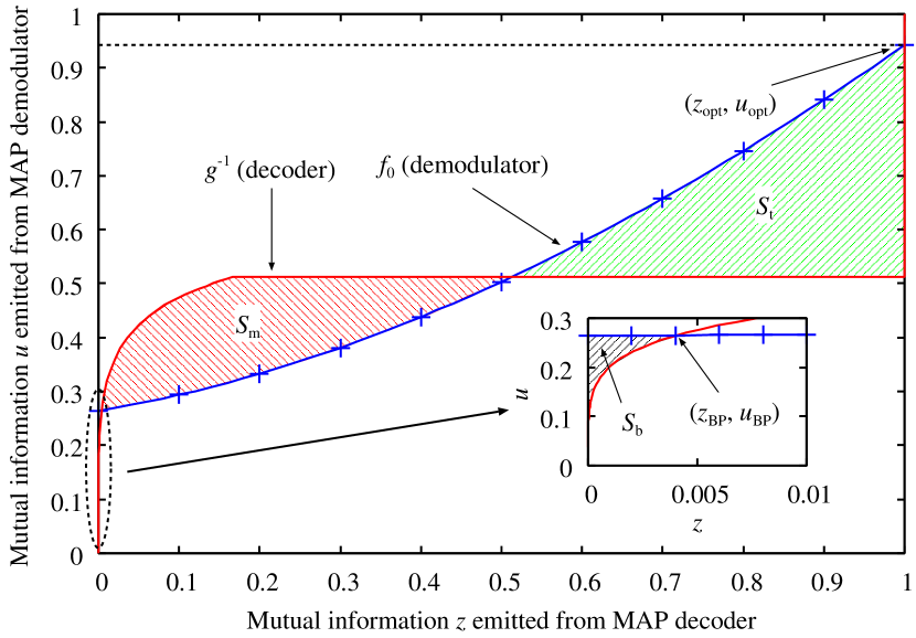
Figure 1: EXIT chart of the conventional BICM-ID with $16$-QAM for erasure extrinsic and AWGN communication channels with an SNR of $5.76$ dB.

Figure 1 shows the EXIT chart for the uncoupled case $W=1$. We used $(3,6)$-LDPC codes, quadrature amplitude modulation (QAM) with $Q=4$ and a symbol mapping proposed in [10], and the additive white Gaussian noise (AWGN) communication channel. We utilized an analytical expression of $g$ for the MAP decoder [11]. In practice, one may use the corresponding SC LDPC code based on BP decoding. We selected a signal-to-noise ratio (SNR) of $5.76$ dB that is slightly larger than the minimum of SNRs such that $u_{\mathrm{opt}}$ is the unique global stable solution of the potential (4) in Theorem 1, so that the SC BICM-ID scheme can approach the target point $(z_{\mathrm{opt}},u_{\mathrm{opt}})=(1,f_{0}(1))$, with $f_{0}(I)=f(I,\ldots,I)$. We find that the FP equations (3) have two stable solutions. One stable solution is the target solution $(z_{\mathrm{opt}},u_{\mathrm{opt}})=(1,f_{0}(1))$, and the other stable solution $(z_{\mathrm{BP}},u_{\mathrm{BP}})$ is a FP to which the BP algorithm converges for the uncoupled case $W=1$. These observations imply that the conventional BICM-ID scheme cannot approach the target point $(1,f_{0}(1))$ in this case, whereas the SC BICM-ID scheme can.

It is possible to understand the performance of the SC BICM-ID scheme from the EXIT chart for the uncoupled case. Let $S_{\mathrm{t}}$, $S_{\mathrm{m}}$, and $S_{\mathrm{b}}$ denote the three areas enclosed by the two curves in Fig. 1 from top to bottom. From the area theorems for the MAP decoder [9], [12, Corollary 5.1] and the MAP demodulator [12, Corollary 5.2], it is straightforward to find the relationship between the areas and the rate loss from the coded modulation (CM) capacity $C_{\mathrm{CM}}$ [12]

$$C_{\mathrm{CM}}-Qr=QS_{\mathrm{b}}+Q(S_{\mathrm{t}}-S_{\mathrm{m}}),$$ (9)

with $r$ denoting the code rate.

Expression (9) implies that the rate loss from the CM capacity is characterized by $S_{\mathrm{b}}$ and $S_{\mathrm{t}}-S_{\mathrm{m}}$. We note that $S_{\mathrm{t}}=S_{\mathrm{m}}$ holds at the BP threshold for conventional SC systems [5]. Since $S_{\mathrm{b}}$ is much smaller than $S_{\mathrm{t}}-S_{\mathrm{m}}$ in Fig. 1, the gap between $S_{\mathrm{t}}$ and $S_{\mathrm{m}}$ is a dominant factor for the rate loss. In fact, the SNR that $S_{\mathrm{t}}=S_{\mathrm{m}}$ holds is approximately $5.29$ dB. Furthermore, the SNR corresponding to the CM capacity is approximately given by $5.12$ dB. Since an SNR of $5.76$ dB was considered in Fig. 1, the losses due to $S_{\mathrm{b}}$ and $S_{\mathrm{t}}-S_{\mathrm{m}}$ are given by $5.29-5.12=0.17$ dB and $5.76-5.29=0.47$ dB, respectively, if $S_{\mathrm{b}}$ is assumed to be identical for the two SNRs $5.29$ dB and $5.76$ dB.

III Proof of Theorem 1

III-A Sketch

The proof of Theorem 1 is a generalization of that in [4]. We shall define a partial differential equation that characterizes the FPs to the DE equations (1) and (2).

$$\frac{\partial\tilde{u}}{\partial t}(x,t)=-\tilde{u}(x,t)+\tilde{\mathfrak{L}}[\tilde{u}(\cdot,t)](x),$$ (10)

where the differential operator $\tilde{\mathfrak{L}}[\tilde{u}](x)$ for any smooth function $\tilde{u}(x)$ on $[-1,1]$ is defined as

$$\tilde{\mathfrak{L}}[\tilde{u}](x)=\varphi_{0}(\psi_{0}(\tilde{u}))+\alpha^{2}\left[A(\tilde{u})\left(\frac{d\tilde{u}}{dx}\right)^{2}+B(\tilde{u})\frac{d^{2}\tilde{u}}{dx^{2}}\right],$$ (11)

with $\tilde{u}$ denoting an abbreviation of $\tilde{u}(x)$. In (11), the two functions $A(\tilde{u})$ and $B(\tilde{u})$ are given by

$$A(\tilde{u})=\frac{\varphi_{0}^{\prime}(\psi_{0}(\tilde{u}))}{6}\left(\bigtriangleup\psi(\tilde{u})+\frac{\bigtriangleup\varphi(\psi_{0}(\tilde{u}))\psi_{0}^{\prime}(\tilde{u})^{2}}{\varphi_{0}^{\prime}(\psi_{0}(\tilde{u}))}+\psi_{0}^{\prime\prime}(\tilde{u})\right),$$ (12)

$$B(\tilde{u})=\frac{1}{3}\varphi_{0}^{\prime}(\psi_{0}(\tilde{u}))\psi_{0}^{\prime}(\tilde{u})>0,$$ (13)

respectively. We impose the boundary condition $\tilde{u}(\pm 1,t)=u_{\mathrm{opt}}$. Furthermore, an initial condition $\tilde{u}(x,0)=\tilde{u}_{\mathrm{init}}(x)$ is imposed with a smooth function $\tilde{u}_{\mathrm{init}}(x)$.

Theorem 2.

There is some initial function $\tilde{u}_{\mathrm{init}}(x)$ such that

$$\lim_{\alpha\to 0}\lim_{i\to\infty}\lim_{W=\alpha L\to\infty}\frac{1}{L}\sum_{l\in\mathcal{L}}\left|u_{l}(i)-\tilde{u}\left(\frac{2l}{L}-1\right)\right|=0,$$ (14)

with $\tilde{u}(x)=\lim_{t\to\infty}\tilde{u}(x,t)$.

Proof:

See Section III-B. ∎

From Theorem 2, it is sufficient to analyze the stationary solution $\tilde{u}(x)$ to the partial differential equation (10), which satisfies

$$\tilde{u}-\varphi_{0}(\psi_{0}(\tilde{u}))=\alpha^{2}\left[A(\tilde{u})\left(\frac{d\tilde{u}}{dx}\right)^{2}+B(\tilde{u})\frac{d^{2}\tilde{u}}{dx^{2}}\right],$$ (15)

with the boundary condition $\tilde{u}(\pm 1)=u_{\mathrm{opt}}$. Theorem 1 follows immediately from the following theorem.

Theorem 3.

If and only if $u_{\mathrm{opt}}$ is the unique global stable solution of the potential (4), the uniform solution $\tilde{u}(x)=u_{\mathrm{opt}}$ is the unique solution to the boundary-value problem (15) in the limit $\alpha\to 0$.

Proof:

We first present a coordinate system that simplifies the representation of the differential system (15). Let us define the change of variables $y=f(\tilde{u})$ by

$$f(\tilde{u})=\int e^{C(\tilde{u})}d\tilde{u},$$ (16)

with

$$C(\tilde{u})=\int\frac{A(\tilde{u})}{B(\tilde{u})}d\tilde{u}.$$ (17)

Calculating $d^{2}y/dx^{2}$ with the chain rule for partial derivative yields

$$\frac{d^{2}y}{dx^{2}}=\frac{e^{C(\tilde{u})}}{B(\tilde{u})}\left[A(\tilde{u})\left(\frac{d\tilde{u}}{dx}\right)^{2}+B(\tilde{u})\frac{d^{2}\tilde{u}}{dx^{2}}\right].$$ (18)

Thus, the differential equation (15) for stationary solutions reduces to

$$\alpha^{2}\frac{d^{2}y}{dx^{2}}(x)=\tilde{V}^{\prime}(y(x)),$$ (19)

where the derivative of a potential $\tilde{V}(y)$ is given by

$$\tilde{V}^{\prime}(y)=\left\{\tilde{u}-\varphi_{0}(\psi_{0}(\tilde{u}))\right\}\frac{e^{C(\tilde{u})}}{B(\tilde{u})},$$ (20)

with $\tilde{u}=f^{-1}(y)$. It is straightforward to confirm that $\tilde{V}^{\prime}(y)=0$ if and only if $\tilde{u}=f^{-1}(y)$ is a solution to the FP equation $\tilde{u}=\varphi_{0}(\psi_{0}(\tilde{u}))$ obtained from (3) for the uncoupled system. In particular, any stable solution to the potential $\tilde{V}$ corresponds to a stable FP to (3). Thus, $y_{\mathrm{opt}}=f(u_{\mathrm{opt}})$ is a stable solution to $\tilde{V}(y)$.

It can be proved that the uniform solution $y(x)=y_{\mathrm{opt}}$ is the unique solution to the boundary-value problem (19) with $y(\pm 1)=y_{\mathrm{opt}}$ if and only if $y_{\mathrm{opt}}$ is the unique global stable solution of $\tilde{V}(y)$. Hassani et al. [13] presented an intuitive explanation of this statement based on classical mechanics. See [14, 4] for a rigorous proof based on the intuition.

Let us prove that the potential $\tilde{V}(y)$ defined via (20) is equivalent to (4). By definition, we use (16) and (20) to obtain

$$\tilde{V}(y)=\int\tilde{V}^{\prime}(y)dy=\int\left\{\tilde{u}-\varphi_{0}(\psi_{0}(\tilde{u}))\right\}\frac{e^{2C(\tilde{u})}}{B(\tilde{u})}d\tilde{u}.$$ (21)

We calculate (17) with (12) and (13) to obtain

$$2C(\tilde{u})= \int\left\{\frac{\bigtriangleup\psi(\tilde{u})}{\psi_{0}^{\prime}(\tilde{u})}+\frac{\bigtriangleup\varphi(\psi_{0}(\tilde{u}))\psi_{0}^{\prime}(\tilde{u})}{\varphi_{0}^{\prime}(\psi_{0}(\tilde{u}))}+\frac{\psi_{0}^{\prime\prime}(\tilde{u})}{\psi_{0}^{\prime}(\tilde{u})}\right\}d\tilde{u}$$

$$= D(\tilde{u};\psi)+D(\psi_{0}(\tilde{u});\varphi)+\ln B(\tilde{u})+\ln\psi_{0}^{\prime}(\tilde{u}),$$ (22)

with (5). Substituting this expression into (21), we arrive at $\tilde{V}(y)=V(f^{-1}(y))$ given by (4). This implies that Theorem 3 holds. ∎

III-B Proof of Theorem 2

We first confirm that the DE equations (1) and (2) are convergent as $i\to\infty$.

Lemma 1.

For any $i$ and $l$, $u_{l}(i)\leq u_{l}(i+1)$ holds.

Proof:

The proof is by induction. The initial condition $u_{l}(0)=u_{\mathrm{min}}$ implies $u_{l}(i)\leq u_{l}(i+1)$ for $i=0$. Suppose that $u_{l}(i)\leq u_{l}(i+1)$ holds for some $i$. Since $\psi$ is increasing in all arguments, from (2) we obtain

$$v_{l}(i+1)-v_{l}(i)$$

$$= \frac{1}{W^{\tilde{d}}}\sum_{\boldsymbol{w}_{\tilde{d}}\in\mathcal{W}^{\tilde{d}}}[\psi(\boldsymbol{u}_{l-\boldsymbol{w}_{\tilde{d}}}(i+1))-\psi(\boldsymbol{u}_{l-\boldsymbol{w}_{\tilde{d}}}(i))]$$

$$\geq 0,$$ (23)

for $l\in\{W-1,\ldots,L-1\}$. Combining (23) and the boundary condition $v_{l}(i)=v_{l}(i+1)=v_{\mathrm{opt}}$ for $l\notin\{W-1,\ldots,L-1\}$, we obtain $v_{l}(i)\leq v_{l}(i+1)$ for all $l$. Repeating the same argument for (1), we arrive at $u_{l}(i+1)\leq u_{l}(i+2)$ for all $l$. By induction, Lemma 1 holds. ∎

Theorem 2 is proved as follows: We first take the continuum limit to reduce the DE equations (1) and (2) to integral systems. Then, we shall derive the differential system (10) by expanding the integral systems with respect to $\alpha$. Finally, we investigate the relationship between stationary solutions for the integral and differential systems as $\alpha\to 0$.

Let us define the integral systems as

$$u(x,i+1)=\frac{1}{(2\alpha)^{d}}\int_{[-\alpha,\alpha]^{d}}\varphi(\boldsymbol{v}(x+\boldsymbol{\omega}_{d},i))d\boldsymbol{\omega}_{d},\;\;|x|\leq 1,$$ (24)

$$v(x,i)=\frac{1}{(2\alpha)^{\tilde{d}}}\int_{[-\alpha,\alpha]^{\tilde{d}}}\psi(\boldsymbol{u}(x-\boldsymbol{\omega}_{\tilde{d}},i))d\boldsymbol{\omega}_{\tilde{d}},\;\;|x|\leq 1-\alpha,$$ (25)

where we have introduced the notation $\boldsymbol{v}(x+\boldsymbol{\omega}_{d},i)=(v(x+\omega_{1},i),\ldots,v(x+\omega_{d},i))$ and $\boldsymbol{u}(x-\boldsymbol{\omega}_{\tilde{d}},i)=(u(x-\omega_{1},i),\ldots,u(x-\omega_{\tilde{d}},i))$, with $\boldsymbol{\omega}_{k}=(\omega_{1},\ldots,\omega_{k})$. We impose the initial condition $u(x,0)=u_{\mathrm{min}}$ for all $|x|\leq 1$. Furthermore, the boundary condition $v(x,i)=v_{\mathrm{opt}}$ is imposed for all $|x|>1-\alpha$ and all $i$. Since the two functions $\varphi$ and $\psi$ have been assumed to be bounded and continuous, the integral systems (24) and (25) are well defined for any $i$.

The integral systems (24) and (25) define a recursive formula $u(x,i+1)=\mathfrak{L}[u(\cdot,i)](x)$ with respect to $u(x,i)$, in which the operator $\mathfrak{L}$ is a counterpart of the differential operator $\tilde{\mathfrak{L}}$ given by (11).

Lemma 2.

1. For any $x$, $i$, and any $\alpha>0$,

   $$u(x,i)\leq u(x,i+1),\quad v(x,i)\leq v(x,i+1).$$ (26)

2. For any $i$ and $l\in\mathcal{L}$,

   $$\lim_{W=\alpha L\to\infty}\frac{1}{L}\sum_{l\in\mathcal{L}}\left|u_{l}(i)-u\left(\frac{2l}{L}-1,i\right)\right|=0,$$ (27)

   $$\lim_{W=\alpha L\to\infty}\frac{1}{L}\sum_{l\in\mathcal{L}}\left|v_{l}(i)-v\left(\frac{2l}{L}-1-\alpha,i\right)\right|=0.$$ (28)

3. For any $i$, $u(x,i)$ is even, continuous on $[-1,1]$, and smooth on $(-1,1)-\{\pm(1-2\alpha)\}$. The stationary solution $u(x)=\lim_{i\to\infty}u(x,i)$ also has the same properties as $u(x,i)$.

Proof:

See [4]. ∎

From the last property of Lemma 2, there exists some smooth initial function $\tilde{u}_{\mathrm{init}}(x)$ that is sufficiently close to the FP $u(x)$ of the integral systems. We impose the initial condition $\tilde{u}(x,0)=\tilde{u}_{\mathrm{init}}(x)$ for the differential system (10) with such an initial function.

We next summarize several properties of the partial differential equation (10).

Lemma 3.

For any $\epsilon>0$ and $x\in[-1,1]$, there exist some $t_{0}>0$ and stationary solution $\tilde{u}(x)$ such that

$$|\tilde{u}(x,t)-\tilde{u}(x)|<\epsilon,$$ (29)

for all $t\geq t_{0}$ and $\alpha>0$.

Proof:

See [4]. ∎

Proposition 1.

Suppose that $u(x)$ is any smooth function on $[-1,1]$. For any $\epsilon>0$, there exists some $\alpha_{0}>0$ such that

$$\int_{-1}^{1}\left|\mathfrak{L}[u](x)-\tilde{\mathfrak{L}}[u](x)\right|dx<\epsilon,$$ (30)

for all $\alpha\in(0,\alpha_{0})$.

Proof:

Let $\mathcal{X}=(-(1-2\alpha),1-2\alpha)$ and $\bar{\mathcal{X}}=[-1,1]\backslash\mathcal{X}$ denote the bulk and boundary regions, respectively. We decompose the integral (30) into two parts.

$$\int_{-1}^{1}\left|\mathfrak{L}[u](x)-\tilde{\mathfrak{L}}[u](x)\right|dx$$

$$= \int_{\mathcal{X}}\left|\mathfrak{L}[u](x)-\tilde{\mathfrak{L}}[u](x)\right|dx+\int_{\bar{\mathcal{X}}}\left|\mathfrak{L}[u](x)-\tilde{\mathfrak{L}}[u](x)\right|dx.$$

It is straightforward to show that the second term tends to zero as $\alpha\to 0$. Thus, we focus on the first term.

To complete the proof of Proposition 1, it is sufficient to prove that the integrand $|\mathfrak{L}[u](x)-\tilde{\mathfrak{L}}[u](x)|$ converges to zero as $\alpha\to 0$ for all $x\in\mathcal{X}$ in the bulk region [4]. Since $u(x)$ is smooth, we can expand $\mathfrak{L}[u](x)$ with respect to $\alpha$ up to the second order. Expanding the integrand in (24) with respect to $\boldsymbol{\omega}_{d}$ yields

$$\mathfrak{L}[u](x)=\varphi_{0}(v)+\frac{\alpha^{2}}{6}\left\{\bigtriangleup\varphi(v)\left(\frac{dv}{dx}\right)^{2}+\varphi_{0}^{\prime}(v)\frac{d^{2}v}{dx^{2}}\right\}+o(\alpha^{2}),$$ (32)

where $v$ is given by the right-hand side (RHS) of (25) with $u(x,i)=u(x)$. Similarly, expanding $v$ with respect to $\alpha$ gives

$$v=\psi_{0}(u)+\frac{\alpha^{2}}{6}\left[\bigtriangleup\psi(u)\left(\frac{du}{dx}\right)^{2}+\psi_{0}^{\prime}(u)\frac{d^{2}u}{dx^{2}}\right]+o(\alpha^{2}),$$ (33)

where $u$ is an abbreviation of $u(x)$. Substituting (33) into (32) and expanding the obtained formula with respect to $\alpha$, we obtain $\mathfrak{L}[u](x)=\tilde{\mathfrak{L}}[u](x)+o(\alpha^{2})$, given by (11). ∎

Lemma 4.

For any $t_{0}>0$ and $\epsilon>0$, there exists some $\alpha_{0}>0$ such that

$$\int_{-1}^{1}|\tilde{u}(x,t_{0})-\tilde{u}(x,0)|dx<\epsilon,$$ (34)

for all $\alpha\in(0,\alpha_{0})$.

Proof:

The proof is based on Proposition 1. See [4] for the details. ∎

We are ready to prove Theorem 2.

Proof:

Let $x_{l}=(2l/L)-1$. Lemma 1 and the first property of Lemma 2 imply that, for any $l\in\mathcal{L}$, $\alpha>0$, and any $\epsilon>0$, there exists some $I\in\mathbb{N}$ such that

$$|u_{l}(i)-u_{l}(I)|<\epsilon,\quad|u(x_{l},i)-u(x_{l})|<\epsilon,$$ (35)

for all $i\geq I$, with $u(x)=\lim_{i\to\infty}u(x,i)$ denoting the stationary solution to the integral systems (24) and (25). With this number $I$ of iterations we use the triangle inequality for the left-hand side (LHS) of (14) to obtain

$$\frac{1}{L}\sum_{l\in\mathcal{L}}|u_{l}(i)-\tilde{u}(x_{l})|< \frac{1}{L}\sum_{l\in\mathcal{L}}|u_{l}(I)-u(x_{l},I)|$$

$$+ \frac{1}{L}\sum_{l\in\mathcal{L}}|u(x_{l})-\tilde{u}(x_{l})|+2\epsilon,$$ (36)

for all $i\geq I$.

From the second property of Lemma 2, we find that the first term on the upper bound (36) tends to zero in the continuum limit $W=\alpha L\to\infty$. From the definition of the Riemann integral, the second term converges to the integral

$$\lim_{W=\alpha L\to\infty}\frac{1}{L}\sum_{l\in\mathcal{L}}|u(x_{l})-\tilde{u}(x_{l})|=\frac{1}{2}\int_{-1}^{1}|u(x)-\tilde{u}(x)|dx.$$ (37)

Thus, it is sufficient to prove that the RHS of (37) tends to zero as $\alpha\to 0$.

For any $\epsilon>0$ and some $t_{0}\in\mathbb{R}$ in Lemma 3, we use the triangle inequality to obtain

$$\frac{1}{2}\int_{-1}^{1}|u(x)-\tilde{u}(x)|dx<\frac{1}{2}\int_{-1}^{1}|u(x)-\tilde{u}(x,t_{0})|dx+\epsilon.$$ (38)

From Lemma 4 and the definition of the initial condition for the differential system (10), the first term on the upper bound (38) converges to zero as $\alpha\to 0$. ∎

References

- [1] S. Kudekar, T. Richardson, and R. Urbanke, “Threshold saturation via spatial coupling: Why convolutional LDPC ensembles perform so well over the BEC,” IEEE Trans. Inf. Theory, vol. 57, no. 2, pp. 803–834, Feb. 2011.
- [2] A. Yedla, Y.-Y. Jian, P. S. Nguyen, and H. D. Pfister, “A simple proof of threshold saturation for coupled scalar recursions,” in Proc. 7th Int. Symp. Turbo Codes & Iter. Inf. Process., Gothenburg, Sweden, Aug. 2012.
- [3] D. L. Donoho, A. Javanmard, and A. Montanari, “Information-theoretically optimal compressed sensing via spatial coupling and approximate message passing,” IEEE Trans. Inf. Theory, vol. 59, no. 11, pp. 7434–7464, Nov. 2013.
- [4] K. Takeuchi, T. Tanaka, and T. Kawabata, “Performance improvement of iterative multiuser detection for large sparsely-spread CDMA systems by spatial coupling,” submitted to IEEE Trans. Inf. Theory, 2012, [Online]. Available: http://arxiv.org/abs/1206.5919.
- [5] S. Kudekar, T. Richardson, and R. Urbanke, “Wave-like solutions of general one-dimensional spatially coupled systems,” submitted to IEEE Trans. Inf. Theory, 2012, [Online]. Available: http://arxiv.org/abs/1208.5273.
- [6] C. Schlegel and M. Burnashev, “Thresholds of spatially coupled systems via Lyapunov’s method,” in Proc. 2013 IEEE Inf. Theory Workshop, Seville, Spain, Sep. 2013.
- [7] K. Takeuchi and S. Horio, “Iterative multiuser detection and decoding with spatially coupled interleaving,” IEEE Wireless Commun. Lett., vol. 2, no. 6, pp. 619–622, Dec. 2013.
- [8] X. Li, A. Chindapol, and J. A. Ritcey, “Bit-interleaved coded modulation with iterative decoding and 8PSK signaling,” IEEE Trans. Commun., vol. 50, no. 8, pp. 1250–1257, Aug. 2002.
- [9] A. Ashikhmin, G. Kramer, and S. ten Brink, “Extrinsic information transfer functions: Model and erasure channel properties,” IEEE Trans. Inf. Theory, vol. 50, no. 11, pp. 2657–2673, Nov. 2004.
- [10] J. Tan and G. L. Stüber, “Analysis and design of symbol mappers for iteratively decoded BICM,” IEEE Trans. Wireless Commun., vol. 4, no. 2, pp. 662–672, Mar. 2005.
- [11] C. Méasson, A. Montanari, and R. Urbanke, “Maxwell construction: The hidden bridge between iterative and maximum a posteriori decoding,” IEEE Trans. Inf. Theory, vol. 54, no. 12, pp. 5277–5307, Dec. 2008.
- [12] A. G. Fàbregas, A. Martinez, and G. Caire, Bit-Interleaved Coded Modulation. Hanover, MA, USA: now Publishers Inc., 2008.
- [13] S. H. Hassani, N. Macris, and R. Urbanke, “Chains of mean field models,” J. Stat. Mech., no. 2, p. P02011, Feb. 2012.
- [14] K. Takeuchi, T. Tanaka, and T. Kawabata, “A phenomenological study on threshold improvement via spatial coupling,” IEICE Trans. Fundamentals, vol. E95-A, no. 5, pp. 974–977, May 2012.