KCL-mth-13-12

YITP-13-129

IPMU13-0237

The Noether-Lefschetz Problem and Gauge-Group-Resolved Landscapes:
F-Theory on ${\rm K3}\times{\rm K3}$ as a Test Case

Andreas P. Braun¹, Yusuke Kimura² and Taizan Watari³

¹Department of Mathematics, King’s College, London WC2R 2LS, UK

²Yukawa Institute for Theoretical Physics, Kyoto University, Kyoto 606-8502, Japan

³Kavli Institute for the Physics and Mathematics of the Universe, University of Tokyo, Kashiwano-ha 5-1-5, 277-8583, Japan

1 Introduction

Flux compactifications of type IIB string theory / F-theory can generate large supersymmetric masses for moduli, so that the moduli particles decay well before the period of big-bang nucleosynthesis. In addition to this phenomenological advantage, the discretum of vacua in this class of compactifications provides an ensemble of vacua (or landscape), which gives rise to a scientific/stringy basis for a notion of naturalness [1, 2]. Certainly the (geometric phase) Calabi–Yau compactifications of type IIB / F-theory are not more than a small subset of all possible vacua in string theory. However, one can still think of some use in such a restricted ensemble of vacua because supersymmetric extensions of the Standard Model and grand unification can be naturally accommodated in this framework.

Given a topological configuration of three-form fluxes in type IIB string theory compactified on a Calabi–Yau threefold $M_{3}$, the dilaton and complex structure moduli of $M_{3}$ are stabilized and their vacuum expectation values (vevs) are determined. By this mechanism, however, not only the moduli vevs (= the coupling constants of the low-energy effective theories), but also a configuration of D7-branes (= (a part of) the gauge group of the effective theories) is determined.

Low-energy effective theories in particle physics are usually crudely classified by such information as gauge groups, matter representations, types of non-vanishing interactions and matter multiplicity, and then the effective theories sharing this information are distinguished by the values of coupling constants. In order to fit this natural framework of thought, ensembles of string flux vacua should also be crudely classified by algebraic and topological information. After this, statistics should be presented in the form of distributions over the moduli space of compactifications sharing the same set of algebraic and topological information. With the statistics of flux vacua presented in this way, we begin to be able to ask such naturalness-related questions as the ratio of the number of vacua having various algebraic and/or topological data or the distribution of various coupling constants (moduli parameters) in a class of theories having a give set of algebraic/topological data. This article aims at taking one step further in this program. The distribution of gauge groups in effective four-dimensional theories derived from string compactifications has been studied from several perspectives in the literature, see [3, 4, 5, 6] for examples.

Stabilization / determination of D7-brane configurations can be understood purely in type IIB language in terms of calibration conditions [7, 8]. Another option is to use F-theory, where the 7-brane configuration, dilaton vev and complex structure moduli of $M_{3}$ are all treated as part of the complex structure moduli of a Calabi–Yau fourfold $Y_{4}$. In F-theory language, there are two ways to understand the mechanism of determination of the moduli vevs. One is to specify the four-form flux on an elliptic fibred Calabi–Yau fourfold $Y$ topologically,

$$[G^{(4)}]\in H^{4}(Y;\mathbb{Z})\,.$$ (1)

The Gukov–Vafa–Witten superpotential

$$W_{\rm GVW}\propto\int_{Y}\Omega_{Y}\wedge G^{(4)}$$ (2)

gives rise to an F-term scalar potential that depends on the complex structure moduli of $Y$. The minimization of this potential determines the vevs of those moduli. Once the moduli vevs arrive at the minimum of the potential (and if the cosmological constant happens to vanish), the four-form flux $G^{(4)}$ is guaranteed to only have a $(2,2)$ component in the Hodge decomposition under the complex structure corresponding to the vevs [12, 13]. In the presence of the four-form flux, the moduli fields slide down the potential to find a vacuum complex structure, so that $[G^{(4)}]$ only has the $(2,2)$ component. If we are to allow large vacuum expectation values of $W_{\rm GVW}$ $[G^{(4)}]$ may also have $(4,0)$ and $(0,4)$ components.

An alternative way to characterize the vacuum choice of the complex structure of $Y$ is available by focussing on the finitely generated Abelian group

$$H^{4}(Y;\mathbb{Z})\cap H^{2,2}(Y;\mathbb{R})\,\qquad\qquad\left({\rm or~{}}H^{4}(Y;\mathbb{Z})\cap H^{2,2}(Y;\mathbb{R})\oplus[H^{4,0}(Y;\mathbb{C})+{\rm h.c}]\right)\,.$$ (3)

The rank of this Abelian group remains constant almost everywhere on the moduli space of the complex structure of $Y$, but it jumps at special loci. In mathematics, this problem—at which loci in the moduli space the rank of this Abelian group jumps, and how it changes there—is known as the Noether–Lefschetz problem. Once we find a point in the Noether–Lefschetz locus and insert four-form flux in the enhanced part of the Abelian group (3), we can no longer go away continuously from the Noether–Lefschetz loci in the moduli space while keeping the flux purely of type $(2,2)$. The higher the codimension of a Noether–Lefschetz locus is in the complex structure moduli space, the more moduli are given masses and stabilized. Therefore, the problem of determination of vacuum complex structure is equivalent to the Noether–Lefschetz problem (e.g., [14]).

This article begins, in Sections 2.2, 4.1, 4.3 and 5.2 in particular, with exploiting this equivalence to see how the Noether–Lefschetz problem in F-theory determines statistics of such things as gauge group, discrete symmetry and moduli vevs. We focus our attention on $K3\times K3$ compactifications of F-theory, as in [20, 21, 22, 15, 23, 17, 24]. This compactification cannot be considered realistic enough for an immediate use in particle physics (e.g. there are no matter curves), but a sufficient complexity is involved in this toy model of landscape to make it suitable for the purpose of clarifying various concepts as well as sharpening technical tools.

In the process of deriving statistics, one cannot avoid asking about the modular group (e.g., [16]). In other words, we have to understand when a pair of seemingly different compactification data actually correspond to the same vacuum in physics. In F-theory we have to introduce some equivalence relation among the space of elliptic fibrations that are admitted by $Y_{4}$, so that the quotient space corresponds to the set of physically distinct vacua. In Section 3.2, we use the duality between heterotic string theory and F-theory, and find that the modulo-isomorphism classification of elliptic fibrations should be adopted. This observation yields two problems. One is purely mathematical: how can we work out the modulo-isomorphism classification of elliptic fibration for a given $Y_{4}$ ? A companion paper by the present authors [25] is dedicated to this problem, with a Calabi–Yau fourfold $Y_{4}$ replaced by a K3 surface, and the results in [25] are reviewed mainly in Section 4.1 in this article. The other problem is how to use such results in mathematics to carry out vacuum counting in physics. We take on this issue in Section 4.2.

Sample statistics, which give us some feeling of what string landscapes can do to answer statistical/naturalness questions in particle physics, are obtained in Sections 4.3 and 5.2.

At the same time, though, the study running up to Section 5.2 in this article along with [25] also hints that it may not be easy to pursue the Noether–Lefschetz problem approach for Calabi–Yau fourfolds which are not as simple as ${\rm K3}\times{\rm K3}$ or K3-fibration over some complex surface. One may of course always use the strategy of computing periods, as done e.g. in [26] in the present context. Of course, this approach has its own technical challenges.

The theory of [27, 28, 2] is a promising direction to go beyond a case-by-case study for different choices of fourfolds $Y$. Therefore, the second theme begins to dominate in Section 5.4 toward the end of this article. Since articles as [28] and [16] seemed to have had applications in Type IIB orientifold compactifications in mind primarily, we clarify how to use the Ashok–Denef–Douglas theory to study statistics of flux vacua in F-theory, with the total ensemble resolved into sub-ensembles according to their algebraic and/or topological data such as gauge groups and matter multiplicity. The presentation in [16] sits in the middle between our discussion up to Section 5.2 and that of [27, 28], and makes it easier to understand how the conceptual issues discussed in the sections up to 5.3 fit into the Ashok–Denef–Douglas theory. Although the presentation in Section 5.4 and Appendix C uses $K3\times K3$ compactification as an example, we tried to phrase it in a way ready for generalization at least to cases with K3-fibred Calabi–Yau fourfolds, and possibly to general F-theory compactifications.

There is also the third theme behind Sections 4.3.2, 5.3 and Appendix B in this article. In the duality between heterotic string theory and F-theory, the dictionary of flux data has been mostly phrased by using the stable degeneration limit of [29, 30]. This was for good reasons, because [31, 32, 33] focused on fluxes in F-theory that are directly responsible for the chirality of non-Abelian (GUT gauge group) charged matter fields on the matter curves. There is an extra algebraic curve in the singular fibre over the matter curve in the F-theory geometry, and a flux can be introduced in this algebraic cycle [32, 33]. For more general flux configurations, however, it is not a priori clear to what extent we can use the $dP_{9}\cup dP_{9}$ limit in the duality dictionary, because $dP_{9}\cup dP_{9}$ is quite different from a K3 surface when it comes to whether two-cycles are algebraic or not. There is the work of [19], indicating that ${\rm U}(1)$ flux associated with an elliptically fibred geometry with an extra section stabilizes some complex structure moduli. Furthermore, the spectral cover description of vector bundles in heterotic string theory [29] did not rule out twisting information $\gamma$ which is more general than (134) for special choices of complex structure. Section 5.3 and the Appendix B provide a comprehensive understanding of this material, generalizing the duality dictionary of the flux data in the literature without relying on the $dP_{9}\cup dP_{9}$ limit. Appendix B also makes a trial attempt of studying how much information of such fluxes can be captured by the $dP_{9}\cup dP_{9}$ limit.

A similar theme has already been studied extensively in the series of papers [34, 35, 36, 37, 38, 39]. It will be interesting to clarify the relation between the logical construction given there and the presentation in this article, but this task is beyond the scope of this present article.

All $K3$ surfaces which appear as solutions in this article have Picard number $20$, which fixes the rank of the total gauge group to be $18$ (this is the ‘geometric’ gauge group, which can still be further broken by fluxes). Whenever the non-abelian part of the gauge group has rank less than $18$, there are ${\rm U}(1)$ factors which are geometrically realized as extra sections of the elliptic fibration. The explicit construction of extra section has been an active research program in recent years. As discussed in [40, 19, 41], sections can be realized by demanding appropriate factorization conditions in the Weierstrass model. A study of fluxes in (a resolution of) the scenario of [40] appeared in [42]. As already discussed in [40], extra sections can equivalently be obtained by realizing the elliptic fibre as a hypersurface in ambient spaces with more than a single toric divisor. This strategy is systematically exploited in [43, 44, 45, 46]. Using toric techniques, in particular the classification of tops, models with $I_{5}$ fibres and extra sections were constructed in [47, 48, 49, 50]. Given a specific embedding of the fibre, one can also use a similar approach as [51], i.e. use Tate’s algorithm, to find all possible degenerations leading to a prescribed gauge group [52]. F-theory compactifications with ${\rm U}(1)$ symmetries also give rise to an interesting interplay between geometry and anomalies of the effective field theory, see [53, 54, 55, 56] for some recent works in this direction.

We regret that we use some mathematical jargon and notations, which are non-standard in the physics literature, without explanations. Sections 2–4 of the mathematical companion paper of the present article [25] should contain the necessary background.

2 Four-Form Flux in M/F-Theory on ${\rm K3}\times{\rm K3}$

2.1 Review of Known Results

Compactification of F-theory on $Y={\rm K3}\times{\rm K3}$ has been studied from various perspectives in the literature. To start off, we begin this section with a review of a result in [17]. Their results are immediate for M-theory compactification down to 2+1-dimensions, but it is clear that we can build a study of F-theory compactification down to 3+1-dimensions by adding extra structure and imposing conditions on top of the discussion for M-theory [17].

When the Calabi–Yau fourfold $Y$ is a product of two K3 surfaces, $S_{1}$ and $S_{2}$, the complex structure moduli space of $Y$, ${\cal M}_{\rm cpx}(Y)$, is the product of the complex structure moduli space of $S_{1}$ and $S_{2}$, ${\cal M}_{\rm cpx}(S_{1})\times{\cal M}_{\rm cpx}(S_{2})$. A discussion of the modular group is postponed to later sections. Over the moduli space of $[h^{3,1}(Y)=h^{1,1}(S_{1})+h^{1,1}(S_{2})=40]$ dimensions, the Hodge decomposition of $H^{4}(Y;\mathbb{C})$ varies, because the decompositions of $H^{2}(S_{1};\mathbb{C})$ and $H^{2}(S_{2};\mathbb{C})$ vary on the moduli spaces of the two K3 surfaces.

$$H^{2,2}(Y;\mathbb{R}) =H^{1,1}(S_{1};\mathbb{R})\otimes H^{1,1}(S_{2};\mathbb{R})+[H^{2,0}(S_{1};\mathbb{C})\otimes H^{0,2}(S_{2};\mathbb{C})+{\rm h.c.}]\,,$$ (4)

$$[H^{4,0}(Y;\mathbb{C})+{\rm h.c.}] =[H^{2,0}(S_{1};\mathbb{C})\otimes H^{2,0}(S_{2};\mathbb{C})+{\rm h.c.}]\,,$$ (5)

where $[V+{\rm h.c.}]$ for a complex vector space $V$ with ${\rm dim}_{\mathbb{C}}V=1$ denotes the corresponding 2-dimensional vector space over $\mathbb{R}$. The Hodge components $[H^{4,0}(Y;\mathbb{C})+{\rm h.c}]$ are also included here for now, partly because the four-form flux with non-vanishing $(4,0)$ and $(0,4)$ components still preserves AdS supersymmetry. The overlap between $H^{2}(S_{1};\mathbb{Z})\otimes H^{2}(S_{2};\mathbb{Z})\subset H^{4}(Y;\mathbb{Z})$ and $H^{2,2}\oplus[H^{4,0}+{\rm h.c.}]$ has the maximal rank, 404, when

$${\rm rank}\left[H^{2}(S_{1};\mathbb{Z})\cap H^{1,1}(S_{1};\mathbb{R})\right]=20,\qquad{\rm rank}\left[H^{2}(S_{2};\mathbb{Z})\cap H^{1,1}(S_{2};\mathbb{R})\right]=20\,.$$ (6)

The loci satisfying these conditions have complex codimension $40$ in the moduli space ${\cal M}_{\rm cpx}(S_{1})\times{\cal M}_{\rm cpx}(S_{2})$, and hence are isolated points. Once plenty of fluxes are introduced in this rank 404 free Abelian group, all the complex structure moduli are stabilized.

The Abelian group

$$S_{X}=\left[H^{1,1}(X;\mathbb{R})\cap H^{2}(X;\mathbb{Z})\right]\subset H^{2}(X;\mathbb{Z})$$ (7)

for a K3 surface $X$ is called Neron–Severi lattice (or group), and the rank of $S_{X}$—denoted by $\rho_{X}$ or $\rho(X)$—is called the Picard number of $X$. $S_{X}$ is empty for $X$ with a generic complex structure, but its rank can be as large as 20, which is possible only in points of ${\cal M}_{\rm cpx}(X)$. K3 surfaces with $\rho_{X}=20$ are called attractive K3 surfaces in [57]. Thus, the ensemble of flux vacua of M-theory/F-theory compactifications on $Y={\rm K3}\times{\rm K3}$ are mapped into a subset of ${\cal M}_{\rm cpx}(S_{1})\times{\cal M}_{\rm cpx}(S_{2})$ where both $S_{1}$ and $S_{2}$ are attractive K3 surfaces.

It is convenient for the classification of K3 surfaces with large Picard number to use the transcendental lattice. For a K3 surface $X$, it is defined as the orthogonal complement of $S_{X}$ under the intersection form in $H^{2}(X;\mathbb{Z})$:

$$T_{X}:=\left[(S_{X})^{\perp}\subset H^{2}(X;\mathbb{Z})\right].$$ (8)

For a K3 surface with Picard number $\rho_{X}$, ${\rm rank}(T_{X})=22-\rho_{X}$. K3 surfaces with a given transcendental lattice form a $(20-\rho_{X})$-dimensional subspace of ${\cal M}_{\rm cpx}({\rm K3})$, and in particular, attractive K3 surfaces are in one-to-one correspondence with rank-2 transcendental lattices (modulo orientation-preserving basis change).

For an attractive K3 surface $X$, its rank-2 transcendental lattice has to be even and positive definite. This is equivalent to the condition that, for a set of generators $\{p,q\}$ of $T_{X}$, the intersection from is given by

$$\left[\begin{array}[]{cc}(p,p)&(p,q)\\ (q,p)&(q,q)\end{array}\right]=\left[\begin{array}[]{cc}2a&b\\ b&2c\end{array}\right],$$ (10)

where $a,b,c$ are all integers, $Q:=4ac-b^{2}$ is positive, and $a,c>0$. The 2-dimensional vector space $T_{X}\otimes\mathbb{C}$ over $\mathbb{C}$ (resp. $T_{X}\otimes\mathbb{R}$ over $\mathbb{R}$) agrees precisely with the vector space $H^{2,0}(X;\mathbb{C})\oplus H^{0,2}(X;\mathbb{C})$ (resp. $[H^{2,0}(X;\mathbb{C})+{\rm h.c.}]$), and the complex vector subspace $H^{2,0}(X;\mathbb{C})\subset T_{X}\otimes\mathbb{C}$ is identified with $\mathbb{C}\cdot\Omega_{X}\subset T_{X}\otimes\mathbb{C}$, where

$$T_{X}\otimes\mathbb{C}\ni\Omega_{X}:=p+\tau q,\qquad\qquad\tau:=\frac{-b+i\sqrt{Q}}{2c}\,.$$ (11)

With orientation-preserving basis changes of $T_{X}$, one can always choose the integers $a,b,c$ such that

$$0\leq|b|\leq c\leq a\qquad({\rm but}\quad 0\leq b\quad{\rm if~{}}c=a)\qquad{\rm and~{}}Q>0\,.$$ (12)

An attractive K3 surface characterized by integers $a,b,c$ in the way explained above is denoted by $X_{[a~{}b~{}c]}$ in this article.

For a pair of attractive K3 surfaces $S_{1}$ and $S_{2}$, let $\{q_{1},p_{1}\}$ and $\{q_{2},p_{2}\}$ be the oriented basis of $T_{S_{1}}$ and $T_{S_{2}}$, respectively. The intersection form in this basis is denoted by

$$\left[\begin{array}[]{cc}(p_{1},p_{1})&(p_{1},q_{1})\\ (q_{1},p_{1})&(q_{1},q_{1})\end{array}\right]=\left[\begin{array}[]{cc}2a&b\\ b&2c\end{array}\right]\,,\qquad\qquad\left[\begin{array}[]{cc}(p_{2},p_{2})&(p_{2},q_{2})\\ (q_{2},p_{2})&(q_{2},q_{2})\end{array}\right]=\left[\begin{array}[]{cc}2d&e\\ e&2f\end{array}\right]\,,$$ (13)

where $a,b,c,d,e$ and $f$ are all integers. The positive definiteness implies that

$$0\leq|b|\leq c\leq a,\qquad({\rm but~{}}0\leq b{\rm~{}if~{}}c=a),\qquad Q_{1}:=4ac-b^{2}>0,$$ (14)

$$0\leq|e|\leq f\leq d,\qquad({\rm but~{}}0\leq e{\rm~{}if~{}}f=d),\qquad Q_{2}:=4df-c^{2}>0,$$ (15)

where all $a,\cdots,f$ are integers. The holomorphic (2,0)-forms on the K3 surfaces $S_{1}=X_{[a~{}b~{}c]}$ and $S_{2}=X_{[d~{}e~{}f]}$ can then be written as

$$\Omega_{S_{1}}=p_{1}+\tau_{1}q_{1},\quad\tau_{1}=\frac{-b+i\sqrt{Q_{1}}}{2c},\qquad\Omega_{S_{2}}=p_{2}+\tau_{2}q_{2},\quad\tau_{2}=\frac{-e+i\sqrt{Q_{2}}}{2f}\,.$$ (16)

Note that $\tau_{1}\in\mathbb{Q}[\sqrt{Q_{1}}]$ and $\tau_{2}\in\mathbb{Q}[\sqrt{Q_{2}}]$. Both $\mathbb{Q}[\sqrt{Q_{1}}]$ and $\mathbb{Q}[\sqrt{Q_{2}}]$ are degree 2 (${\cal D}=2$) algebraic extensions of $\mathbb{Q}$ (see Ref. [57]).

In physics applications, we would rather like to impose one more condition. The M2/D3-brane tadpole cancellation is equivalent to

$$\frac{1}{2}\int_{Y}(G\wedge G)+N_{M2/D3}=\frac{\chi(Y)}{24}=24\,,$$ (17)

where $N_{M2/D3}$ is the number of M2/D3-branes minus anti-M2/D3-branes (that are point like) in $Y$. When we exclude anti M2/D3-branes on $Y$, $N_{M2/D3}\geq 0$, and thus not all the pairs of attractive K3 surfaces in ${\cal M}_{\rm cpx}(S_{1})\times{\cal M}_{\rm cpx}(S_{2})$ qualify for the landscape of flux vacua of M-theory compactified on $Y={\rm K3}\times{\rm K3}$.

Aspinwall and Kallosh carried out an explicit study of which pairs of attractive K3 surfaces can satisfy the condition (17), within a couple of constraints that make the analysis easier [17]. In order to state one of the constraints introduced in [17], we need the following definition. Let us focus on a pair of attractive K3 surfaces $S_{1}$ and $S_{2}$. Any $G^{(4)}$ in (3) on $Y=S_{1}\times S_{2}$ can be decomposed, under the Hodge structure of $Y$, into $[G]=[G_{1}]+[G_{0}]$, where

$$[G_{0}] \in\left[H^{1,1}(S_{1};\mathbb{R})\otimes H^{1,1}(S_{2};\mathbb{R})\right]=S_{S_{1}}\otimes S_{S_{2}}\otimes\mathbb{R},$$ (18)

$$[G_{1}] \in\left[H^{2,0}(S_{1};\mathbb{C})\otimes H^{0,2}(S_{2};\mathbb{C})+{\rm h.c.}\right],$$ (19)

$$\qquad\left({\rm or}\qquad\in\left[H^{2,0}(S_{1};\mathbb{C})+{\rm h.c.}\right]\otimes\left[H^{2,0}(S_{2};\mathbb{C})+{\rm h.c.}\right]=T_{S_{1}}\otimes T_{S_{2}}\otimes\mathbb{R}\right)\,.$$ (20)

The explicit study in Ref. [17] assumes that

$$[G_{0}]=0,$$ (21)

and $[G_{1}]\neq 0$ is that of (19) rather than (20), so that $G^{(4)}=G_{1}$ is purely of $(2,2)$ type in the Hodge structure of $Y=S_{1}\times S_{2}$, and the vev of $W_{\rm GVW}$ vanishes. Another assumption is to set

$$N_{M2/D3}=0\,,$$ (22)

so that

$$\frac{1}{2}[G_{1}]\cdot[G_{1}]=24\,.$$ (23)

Under these constraints, $[G_{1}]$ has to be an integral element of $T_{S_{1}}\otimes T_{S_{2}}$:

$$[G_{1}]\in[H^{2,0}(S_{1};\mathbb{C})\otimes H^{0,2}(S_{2};\mathbb{C})+{\rm h.c.}]\cap(T_{S_{1}}\otimes T_{S_{2}}).$$ (24)

It is not always guaranteed for any pair of attractive K3 surfaces $S_{1}$ and $S_{2}$ that there can be $[G_{1}]\neq 0$. The Abelian group on the right hand side of (24) can be empty. Writing down $[G_{1}]$ as

$$[G_{1}]={\rm Re}\left(\gamma\Omega_{S_{1}}\wedge\overline{\Omega}_{S_{2}}\right)\,$$ (25)

for some $\gamma\in\mathbb{C}$ and expanding this in the integral basis $\{p_{1}\otimes p_{2},\;q_{1}\otimes p_{2},\;p_{1}\otimes q_{2},\;q_{1}\otimes q_{2}\}$ of $T_{S_{1}}\otimes T_{S_{2}}$, Aspinwall and Kallosh found that (24) is non-empty if and only if

$${}^{\exists}m\in\mathbb{Z}\quad{\rm s.t.}\quad Q_{1}Q_{2}=m^{2}\,.$$ (26)

This implies that the two algebraic number fields $\mathbb{Q}[\sqrt{Q_{1}}]$ and $\mathbb{Q}[\sqrt{Q_{2}}]$ are the same. All the period integrals of the holomorphic (4,0) form $\Omega_{Y}=\Omega_{S_{1}}\wedge\Omega_{S_{2}}$ take values in the common degree-2 (${\cal D}=2$) algebraic extension field $\mathbb{Q}[\sqrt{Q_{1}}]$ of $\mathbb{Q}$ (c.f. [16]).

[a b c]	[d e f]	$\gamma$		[a b c]	[d e f]	$\gamma$
[8 8 8]	[1 1 1]	$\gamma^{(6)}$		[6 0 6]	[1 0 1]	$\gamma^{(4)}$
[6 0 3]	[2 0 1]	$\pm i/\sqrt{2}$		[6 0 2]	[3 0 1]	$\pm i/\sqrt{3}$
[6 0 2]	[1 1 1]	$\gamma^{(6)}$		[6 0 1]	[6 0 1]	$\pm i/\sqrt{6}$
[4 4 4]	[2 2 2]	$\gamma^{(6)}$		[3 0 3]	[2 0 2]	$\gamma^{(4)}$
[3 0 3]	[1 0 1]	$(1+i)\gamma^{(4)}$		[3 0 2]	[3 0 2]	$\pm i\sqrt{2/3}$
[3 0 1]	[2 2 2]	$\gamma^{(6)}$		[2 2 2]	[1 1 1]	$2\times\gamma^{(6)}$
[2 0 1]	[2 0 1]	$\pm 1\pm i/\sqrt{2}$

Table 1: Table 1 of Ref. [17] is reproduced here (with minor modifications) for the convenience of the reader. Intersection forms (13) of $T_{S_{1}}$ and $T_{S_{2}}$ are simply denoted by [a b c] and [d e f] in this table. All the possible choices of $\gamma\in\mathbb{C}$ are listed; $\gamma^{(6)}:=\left\{\pm 2i/\sqrt{3},\pm 1\pm i/\sqrt{3}\right\}=2i/\sqrt{3}\times\{e^{2\pi ik/6}|k=0,1,2,3,4,5\}$, $\gamma^{(4)}:=\left\{\pm 1,\pm i\right\}=\{e^{2\pi ik/4}|k=0,1,2,3\}$.

Imposing the condition (23) on $[G_{1}]$ in (24), [17] worked out the complete list of pairs of attractive K3 surfaces where there exists a flux $G^{(4)}$ satisfying (21, 24, 23). The result are 13 pairs of attractive K3 surfaces [17], which are listed in Table 1 along with all possible values of $\gamma\in\mathbb{C}$.

Two remarks are in order here. First note that for a supersymmetric compactification of M-theory on $Y=S_{1}\times S_{2}$ with a four-form flux $G^{(4)}=G_{1}$, we could think of a compactification on $\overline{Y}=\overline{S_{1}}\times\overline{S}_{2}$ obtained by simply declaring that the holomorphic local coordinates on $Y$ are anti-holomorphic coordinates on $\overline{Y}$, keeping the underlying real-8-dimensional manifold the same. The flux $[G_{1}]\in H^{4}(Y;\mathbb{Z})$ remains the same. This new compactification, however, should not be regarded as a vacuum physically different from the original one, only the role of the superpotential and its hermitian conjugate, and that of chiral multiplets and anti-chiral multiplets in the low-energy effective theory, are exchanged. The physics remains the same.

The transcendental lattice of the K3 surface $S^{\prime}_{1}=\overline{S}_{1}$ can be regarded as $T_{S^{\prime}_{1}}\cong{\rm Span}_{\mathbb{Z}}\{p^{\prime}_{1},q^{\prime}_{1}\}:={\rm Span}_{\mathbb{Z}}\{p_{1},-q_{1}\}$, where the symmetric pairing is described by [a’ b’ c’] = [a -b c]. The holomorphic $(2,0)$-form is given by

$$\Omega_{S^{\prime}_{1}}=p^{\prime}_{1}+\tau^{\prime}_{1}q^{\prime}_{1}:=p_{1}+\bar{\tau}_{1}q_{1}=\overline{\Omega}_{S_{1}}.$$ (27)

Thus, the four-form flux $G_{1}={\rm Re}[\gamma\Omega_{S_{1}}\wedge\overline{\Omega}_{S_{2}}]$ is rewritten in terms of $S^{\prime}_{1}\times S^{\prime}_{2}=\overline{S}_{1}\times\overline{S}_{2}$ as $G_{1}={\rm Re}[\gamma^{*}\Omega_{S^{\prime}_{1}}\wedge\overline{\Omega}_{S^{\prime}_{2}}]$. Thus, $Y=S_{1}\times S_{2}$ compactification with [a b c], [d e f] and $\gamma$ and another compactification with [a -b c] and [d -e f] and $\gamma^{*}$ are completely equivalent, and should not be regarded as different compactifications (or different vacua). For this reason, only one of each such pairs is shown in Table 1.

Secondly, as for M-theory compactification, $Y=S_{1}\times S_{2}$ with $G_{1}={\rm Re}(\gamma\Omega_{S_{1}}\wedge\overline{\Omega}_{S_{2}})$ and $Y=S_{2}\times S_{1}$ with $G_{1}={\rm Re}(\gamma^{*}\Omega_{S_{2}}\wedge\overline{\Omega}_{S_{1}})$ should also be regarded equivalent. Thus, Table 1 only shows cases where $a\geq d$, and furthermore, in cases with $a=d$, we impose $c\geq f$.

2.2 Extending the List

Before proceeding to the next section, it is worthwhile to extend the list so that the condition (23) is relaxed to

$$\frac{1}{2}[G_{1}]\cdot[G_{1}]\leq 24.$$ (28)

Certainly for any compactification of M-theory over $Y=S_{1}\times S_{2}$ with a four-form flux $[G_{1}]$ in (24) satisfying the inequality above, at least we can introduce an appropriate number of M2-branes to satisfy the tadpole condition (17). One might even be able to find a flux $[G_{0}]\in(S_{S_{1}}\otimes S_{S_{2}})$ to satisfy (17). See Section 5 for more about the case with $[G_{0}]\neq 0$, however.

Straightforward analysis allows us to extend Table 1, so that it contains all pairs of attractive K3 surfaces $S_{1}$ and $S_{2}$ and a choice of $\gamma\in\mathbb{C}$ satisfying (21, 24) and (28), rather than (21, 24) and (23). The result of our analysis is presented in Table 2.

flux	[a b c]	[d e f]	$\gamma$	M	F
24	[8 8 8]	[1 1 1]	$\gamma^{(6)}$	6	6
	[6 0 6]	[1 0 1]	$\gamma^{(4)}$	3	3
	[6 0 3]	[2 0 1]	$\pm i/\sqrt{2}$	1	1
	[6 0 2]	[3 0 1]	$\pm i/\sqrt{3}$	1	1
	[6 0 2]	[1 1 1]	$\gamma^{(6)}$	6	6
	[6 0 1]	[6 0 1]	$\pm i/\sqrt{6}$	1	1
	[4 4 4]	[2 2 2]	$\gamma^{(6)}$	6	6
	[3 0 3]	[2 0 2]	$\gamma^{(4)}$	3	3
	[3 0 3]	[1 0 1]	$(1+i)\gamma^{(4)}$	2	2
	[3 0 2]	[3 0 2]	$\pm i\sqrt{2/3}$	1	1
	[3 0 1]	[2 2 2]	$\gamma^{(6)}$	6	6
	[2 2 2]	[1 1 1]	$2\gamma^{(6)}$	6	6
	[2 0 1]	[2 0 1]	$\pm 1\pm i/\sqrt{2}$	2	2
23	[6 1 1]	[6 1 1]	$\pm 2i/\sqrt{23}$	1	2
	[3 1 2]	[3 1 2]	$\pm 4i/\sqrt{23}$	1	2
22	[6 2 2]	[3 1 1]	$\pm 2i/\sqrt{11}$	2	2
21	[7 7 7]	[1 1 1]	$\gamma^{(6)}$	6	6
	[6 3 3]	[2 1 1]	$\pm 2i/\sqrt{7}$	2	2
	[1 1 1]	[1 1 1]	$(2\pm\sqrt{3}i)\gamma^{(6)}$	6	12
20	[5 0 5]	[1 0 1]	$\gamma^{(4)}$	3	3
	[5 0 1]	[5 0 1]	$\pm i/\sqrt{5}$	1	1
	[3 2 2]	[3 2 2]	$\pm 2i/\sqrt{5}$	1	2
	[1 0 1]	[1 0 1]	$(1\pm 2i)\gamma^{(4)}$	4	4
19	[5 1 1]	[5 1 1]	$\pm 2i/\sqrt{19}$	1	2
18	[6 6 6]	[1 1 1]	$\gamma^{(6)}$	6	6
	[3 3 3]	[2 2 2]	$\gamma^{(6)}$	6	6
	[2 2 2]	[1 1 1]	$2\gamma^{(6)}$	6	6
17
16	[4 0 4]	[1 0 1]	$\gamma^{(4)}$	3	3
	[4 0 2]	[2 0 1]	$\pm i/\sqrt{2}$	1	1
	[4 0 1]	[4 0 1]	$\pm i/2$	1	1
	[4 0 1]	[1 0 1]	$\gamma^{(4)}$	3	3
	[2 0 2]	[2 0 2]	$\gamma^{(4)}$	3	3
	[2 0 2]	[1 0 1]	$(1+i)\gamma^{(4)}$	2	2
	[2 0 1]	[2 0 1]	$\pm 1$	2	2
	[1 0 1]	[1 0 1]	$2\gamma^{(4)}$	3	3

flux	[a b c]	[d e f]	$\gamma$	M	F
15	[5 5 5]	[1 1 1]	$\gamma^{(6)}$	6	6
	[4 1 1]	[4 1 1]	$\pm 2i/\sqrt{15}$	1	2
	[2 1 2]	[2 1 2]	$\pm 4i/\sqrt{15}$	1	2
14	[4 2 2]	[2 1 1]	$\pm 2i/\sqrt{7}$	2	2
	[2 1 1]	[2 1 1]	$\pm 1\pm i/\sqrt{7}$	*2	4
13
12	[4 4 4]	[1 1 1]	$\gamma^{(6)}$	6	6
	[3 0 3]	[1 0 1]	$\gamma^{(4)}$	3	3
	[3 0 1]	[3 0 1]	$\pm i/\sqrt{3}$	1	1
	[3 0 1]	[1 1 1]	$\gamma^{(6)}$	6	6
	[2 2 2]	[2 2 2]	$\gamma^{(6)}$	3	6
	[1 1 1]	[1 1 1]	$2\gamma^{(6)}$	3	6
11	[3 1 1]	[3 1 1]	$\pm 2i/\sqrt{11}$	1	2
10
9	[3 3 3]	[1 1 1]	$\gamma^{(6)}$	6	6
	[1 1 1]	[1 1 1]	$\sqrt{3}i\gamma^{(6)}$	3	6
8	[2 0 2]	[1 0 1]	$\gamma^{(4)}$	3	3
	[2 0 1]	[2 0 1]	$\pm i/\sqrt{2}$	1	1
	[1 0 1]	[1 0 1]	$(1+i)\gamma^{(4)}$	2	2
7	[2 1 1]	[2 1 1]	$\pm 2i/\sqrt{7}$	1	2
6	[2 2 2]	[1 1 1]	$\gamma^{(6)}$	6	6
5
4	[1 0 1]	[1 0 1]	$\gamma^{(4)}$	3	3
3	[1 1 1]	[1 1 1]	$\gamma^{(6)}$	3	6
flux	[a b c]	[d e f]	$\gamma$	M	F
23	[6 -1 1]	[6 1 1]	$\pm 2i/\sqrt{23}$	2	2
22	[3 -1 1]	[6 2 2]	$\pm 2i\sqrt{11}$	2	2
21	[2 -1 1]	[6 3 3]	$\pm 2i/\sqrt{7}$	2	2
20	[3 -2 2]	[3 2 2]	$\pm 2i/\sqrt{5}$	2	2
19	[5 -1 1]	[5 1 1]	$\pm 2i/\sqrt{19}$	2	2
15	[4 -1 1]	[4 1 1]	$\pm 2i/\sqrt{15}$	2	2
14	[2 -1 1]	[2 1 1]	$\pm 1\pm i/\sqrt{7}$	*4	4
	[2 -1 1]	[4 2 2]	$\pm 2i/\sqrt{7}$	2	2
11	[3 -1 1]	[3 1 1]	$\pm 2i/\sqrt{11}$	2	2
7	[2 -1 1]	[2 1 1]	$\pm 2i/\sqrt{7}$	2	2

Table 2: This table reproduces all the 13 cases with the total flux of $G_{1}$ type being 24 in [17]. The first 5/6 of this table covers the cases with $be\geq 0$; see comments at the end of Section 2.1. The last 1/6 of this table is the list of cases with $(be)<0$; this table only shows cases with $b<0$ (so $e>0$), in order to reduce the redundant information associated with $S_{2}\longleftrightarrow S_{1}$ and $\gamma\longleftrightarrow\gamma^{*}$. See Section 4.2 for the meaning of the last two columns.

Out of the 66 entries in Table 2, some pairs of K3 surfaces appear more than once. In these cases, there are different possible choices of $\gamma$ which give rise to different contributions to the tadpole that are less than $24$. For the pairs $S_{1}\times S_{2}=X_{[1~{}0~{}1]}\times X_{[1~{}0~{}1]}$ and $X_{[1~{}1~{}1]}\times X_{[1~{}1~{}1]}$, all the possible values of $\gamma\in\mathbb{C}$ (and the corresponding $[G_{1}]\cdot[G_{1}]/2$ contribution to the M2/D3 tadpole) are shown in Figure 1.

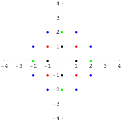
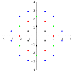
(a) for $X_{[1~{}0~{}1]}\times X_{[1~{}0~{}1]}$		(b) for $X_{[1~{}1~{}1]}\times X_{[1~{}1~{}1]}$

Figure 1: Possible values of $\gamma\in\mathbb{C}$ appearing in Table 2 for $X_{[1~{}0~{}1]}\times X_{[1~{}0~{}1]}$ and $X_{[1~{}1~{}1]}\times X_{[1~{}1~{}1]}$, respectively. In (a), black, red, green and blue points (from inside to outside) correspond to $[G_{1}]\cdot[G_{1}]/2=4,8,16$ and $20$, respectively, while in (b), the black, red, green and blue points give rise to the contributions $3,9,12$ and $21$, respectively.

They form a lattice within $\mathbb{C}$, and so do $[G_{1}]$ in (24) [57]. In fact, one can show that that the possible values for $\gamma$ form a lattice for any pair of K3 surfaces satisfying (26). The upper bound (28), however, allows only finitely many choices of $G^{(4)}=G_{1}$ for a given pair of attractive K3 surfaces satisfying (26).

3 F-theory Classification of Elliptic Fibrations on a K3 Surface

The study reviewed in the previous section implies that a pair of K3 surfaces $S_{1}$ and $S_{2}$ corresponding to a pair of transcendental lattices $T_{S_{1}}=\left[\begin{array}[]{cc}2a&b\\ b&2c\end{array}\right]$ and $T_{S_{2}}=\left[\begin{array}[]{cc}2d&e\\ e&2f\end{array}\right]$ in Tables 1 and 2 is realized in the landscape of flux compactifications of M-theory on $Y=S_{1}\times S_{2}$ down to 2+1-dimensions, with all the 40 complex structure moduli stabilised. In order to translate this result to the landscape of F-theory compactifications to 3+1-dimensions, however, we have to impose a couple of extra conditions [17].

One of the conditions to be imposed, of course, is that either one of the K3 surfaces $S_{1}$ or $S_{2}$ admits an elliptic fibration with a section (in its vacuum complex structure), and the vev of the Kähler moduli should be such that the volume of the elliptic fibre vanishes. Let $X$ be this elliptic fibred K3 surface, and the other one of $S_{1}$ and $S_{2}$ be denoted by $S$;

$$Y=X\times S,\qquad\pi_{X}:X\rightarrow\mathbb{P}^{1},\qquad\sigma:\mathbb{P}^{1}\rightarrow X.$$ (29)

The authors of [17] pointed out that $S_{1}$ (resp. $S_{2}$) can be identified with a K3 surface of the form $X=T^{4}/\mathbb{Z}_{2}$, if and only if all of a, b and c (resp. d, e and f) in Table 1 are even (the same rule applies also to Table 2), based on a known fact on Kummer surfaces (see [61, 59, 62]). Projecting down to $T^{2}/\mathbb{Z}_{2}\simeq\mathbb{P}^{1}$, we obtain an elliptic fibration with four singular fibres of type $I^{*}_{0}$ (namely, $D_{4}=\mathop{\rm SO}(8)$ gauge groups on 7-branes); this is the F-theory/Type IIB orientifold model in [63].

This class of F-theory vacua, which admits a type IIB orientifold interpretation without any approximation or ambiguity, is only a subset of all possible vacua of F-theory, however. In fact, it is known that any K3 surface with $\rho\geq 13$ admits an elliptic fibration with a section (Lemma 12.22 of [64]). Hence all the K3 surfaces in Tables 1 and 2 admit an elliptic fibration with a section, so that they all have an interpretation in terms of F-theory if the vev of the Kähler moduli is chosen appropriately. It should be noted, however, that there can be more than one elliptic fibration morphism $\pi_{X}:X\longrightarrow\mathbb{P}^{1}$ for a given K3 surface $X$, and furthermore, the type of singular fibres (type = collection of some of $I_{n}$, $I^{*}_{n}$, II, III, IV^∗, III^∗ and II^∗) will in general be different for each of the fibrations. We are thus facing at least two questions:

• How do we find out the list of all possible elliptic fibrations, when the transcendental lattice $T_{X}\subset H^{2}(X;\mathbb{Z})$ of a K3 surface $X$ is given?

• Suppose that there are two elliptic fibrations $\pi_{X}:X\longrightarrow\mathbb{P}^{1}$ and $\pi^{\prime}_{X}:X\longrightarrow\mathbb{P}^{1}$ available; how do we find out whether the two fibrations correspond to the same vacuum in physics or not?

The former question is purely mathematical in nature, while the latter is a question in physics. Our companion paper [25] is dedicated to a study of the first question, while the latter question is addressed in this section. The primary conclusion in this section is (51) and the discussion that follows immediately after. We begin by reviewing Torelli theorem for K3 surface in Section 3.1, as it plays a crucial role in our discussion in Section 3.2.

3.1 On the Torelli theorem for K3 surfaces

In this we discuss the relation between the moduli space of complex structures of K3 surfaces and periods of the holomorphic $(2,0)$ form. Statements of this type are generally referred to as ‘Torelli theorems’. For K3 surfaces, there exist several powerful versions, which are closely related to each other, yet shed light on the subject from slightly different angles. Those Torelli theorems combined allow many questions on K3 moduli to be reformulated in terms of lattice theory. The following review on Torelli theorems for K3 surfaces is designed to serve as preparation for Section 3.2. This review together with Section 2 of [25] is designed to be self-contained, all the jargon and notation without definition or explanation in this section should be explained in Section 2 of [25]. See also [65, 62] for a concise mathematical exposition.

We begin with defining such words as “(moduli space of) marked K3 surface” and “period domain”, and proceed to explain the period map. A marked K3 surface is a K3 surface $X$ for which we have fixed a set of generators for $H^{2}(X;\mathbb{Z})$, i.e. we consider a pair $(X,\varphi)$ which consists of the K3 surface $X$ and an isometry between lattices $\varphi:H_{2}(X;\mathbb{Z})\longrightarrow\Lambda_{\rm K3}$, where

$$\Lambda_{\rm K3}=U\oplus U\oplus U\oplus E_{8}\oplus E_{8}\,.$$ (30)

The map $\varphi$ is called the marking. Note that we use conventions in which the $A$–$D$–$E$ lattices have a negative definite inner product, as is natural in the present context.

Two marked K3 surfaces $(X,\varphi)$ and $(X^{\prime},\varphi^{\prime})$ are said to be equivalent, if and only if there is an isomorphism $f:X\rightarrow X^{\prime}$ such that $\varphi^{\prime}\cdot f_{*}=\varphi$ as an isometry from $H_{2}(X;\mathbb{Z})$ to $\Lambda_{\rm K3}$. Each point of the moduli space of marked K3 surface $N$ corresponds to such an equivalence class of marked K3 surfaces.

The period domain $D$, on the other hand, is a subspace of $\mathbb{P}[\Lambda_{\rm K3}\otimes\mathbb{C}]$ given by

$$D:=\{[\omega]\in\mathbb{P}[\Lambda_{\rm K3}\otimes\mathbb{C}]\;|\;\omega\cdot\omega=0,\;\omega\cdot\overline{\omega}>0\;\}\subset\mathbb{P}[\Lambda_{\rm K3}\otimes\mathbb{C}]\,.$$ (31)

The global structure of $D$ is given by

$$D\cong O(\Lambda_{\rm K3}\otimes\mathbb{R})/{\rm SO}(2)\times O(1,19)={\rm Gr}^{\rm po}(2;\Lambda_{\rm K3}\otimes\mathbb{R})\,,$$ (32)

where the superscript “po” stands for “positive and oriented”, in the sense that we consider the Grassmannian of oriented 2-dimensional subspaces in $\Lambda_{\rm K3}\otimes\mathbb{R}$ with signature $(2,0)$.

Using the holomorphic $(2,0)$-form $\Omega_{X}\in H_{2}(X;\mathbb{C})$ and the intersection form on $H_{2}(X;\mathbb{C})$, we may map a point in the moduli space of marked K3 surface $N$ to a point in the period domain $D$:

$${\cal P}:N\ni[(X,\varphi)]\longmapsto\varphi([\Omega_{X}])\in D\subset\mathbb{P}[\Lambda_{\rm K3}\otimes\mathbb{C}]\,.$$ (33)

${\cal P}$ is called the period map. Here, $[\Omega_{X}]$ stands for both the complex line $\mathbb{C}\Omega_{X}\subset H_{2}(X;\mathbb{C})$ as well as its image in $\mathbb{P}[H_{2}(X;\mathbb{C})]$; the same notation has already been used in (31).

The classic local Torelli theorem for K3 surface states that the period map is locally an isomorphism between $N$ and $D$. For any point in $N$ and its image under the period map in $D$, we can always take an appropriate open set in $N$ and $D$ so that the period map becomes an isomorphism between the two open sets. Thus, locally in the moduli space(s), K3 surfaces are uniquely determined by their periods.

In the following, we will turn to global aspects of the moduli spaces $N$ and $D$, and the period map ${\cal P}$ between them. While it turns out that complex deformations can be used to introduce local coordinates on $N$, and to give it the structure of a complex manifold, the moduli space $N$ fails to be Hausdorff. The way the period maps glue globally is expressed by the

Global Torelli Theorem, version 1 (see e.g. [65]): the moduli space of marked K3 surfaces $N$ consists of two connected components $N^{o}$ and $N^{o^{\prime}}$, and the period map ${\cal P}$ maps each one of them surjectively, and also generically injectively to the period domain $D$.

To elaborate more on this, note first that the group of all the isometries of the lattice $\Lambda_{\rm K3}$—${\rm Isom}(\Lambda_{\rm K3})$—acts naturally on $D$ (from the left), and it also acts on $N$ through the marking; $g\in{\rm Isom}(\Lambda_{\rm K3})$ maps $[(X,\varphi)]\in N$ to $[(X,g\cdot\varphi)]\in N$. The action of this symmetry group on $N$ and $D$ commutes with the period map ${\cal P}:N\longrightarrow D$. This isometry group has a structure ${\rm Isom}(\Lambda_{\rm K3})\cong\{\pm{\rm id.}\}\times{\rm Isom}^{+}(\Lambda_{\rm K3})$. The ${\rm Isom}^{+}(\Lambda_{\rm K3})$ subgroup is such that the orientation of the 3-dimensional positive definite subspace of $\Lambda_{\rm K3}\otimes\mathbb{R}$ is preserved.

A pair of elements $[(X,\varphi)]$ and $[(X,-\varphi)]$ are different points in $N$ because automorphisms of $X$ cannot induce $(-{\rm id.})$ on $H_{2}(X;\mathbb{C})$. The period map ${\cal P}:N\longrightarrow D$ sends these two elements to the same point in $D$, $[\varphi(\Omega_{X})]=[-\varphi(\Omega_{X})]\in\mathbb{P}[\Lambda_{\rm K3}\otimes\mathbb{C}]$. In the Torelli theorem above, such a pair of points in $N$ corresponds to two inverse images of a given point in $D$; one is in $N^{o}$, and the other is in the other connected component $N^{{}^{\prime}o}$. The action of $(-{\rm id.})\in{\rm Isom}(\Lambda_{\rm K3})$ maps these two elements in $N$ to each other, and hence the subgroup $\{\pm{\rm id.}\}$ of ${\rm Isom}(\Lambda_{\rm K3})$ acts trivially on $D$, while it exchanges the two connected components of $N$.

Next we discuss the classical form of the global Torelli theorem. First, the homomorphism ${\rm Aut}(X)\longrightarrow{\rm Isom}(H_{2}(X;\mathbb{Z}))$ is injective (Prop. 2 of §2 in [61]), where ${\rm Aut}(X)$ is the group of automorphisms of a K3 surface $X$, and ${\rm Isom}(H_{2}(X;\mathbb{Z}))$ is the isometry group of $H_{2}(X;\mathbb{Z})$ endowed with a symmetric pairing from intersection number. Note that this means that there cannot be any non-trivial automorphism which acts as the identity on $H_{2}(X;\mathbb{Z})$. Furthermore,

Global Torelli Theorem, version 2: (Prop. of §7 and Thm. 1 of §6 in [61]) the image of ${\rm Aut}(X)$ under the injective homomorphism is ${\rm Isom}(H_{2}(X;\mathbb{Z}))^{({\rm Hodge~{}eff})}$, the group of isometries that are both Hodge and effective. This means that for a given $\varphi\in{\rm Isom}(H_{2}(X;\mathbb{Z}))^{({\rm Hodge~{}eff})}$, there exists a unique automorphism $f\in{\rm Aut}(X)$ such that $\varphi=f_{*}$. Furthermore, the subgroup ${\rm Isom}(H_{2}(X;\mathbb{Z}))^{({\rm Hodge~{}eff.})}\cong{\rm Aut}(X)$ sits inside the group of Hodge isometries, which have the form

$${\rm Isom}\left(H_{2}(X;\mathbb{Z})\right)^{({\rm Hodge})}\cong\{\pm{\rm id.}\}\times\left[W^{(2)}(S_{X})\rtimes{\rm Aut}(X)\right]\,.$$ (34)

For K3 surfaces $X$ and $X^{\prime}$ there is an isomorphism of surfaces $f:X\longrightarrow X^{\prime}$ if and only if there is a Hodge and effective isometry $\varphi:H_{2}(X;\mathbb{Z})\longrightarrow H_{2}(X^{\prime};\mathbb{Z})$. In this case, $f_{*}=\varphi$.

See the mathematics literature (such as [61]) or [25] for the definition of Hodge and effective isometries. $W^{(2)}(S_{X})$ is the group generated by reflections associated with algebraic curves of self-intersection $(-2)$ in the Neron–Severi lattice $S_{X}$. Section 2.2 of [25] explains the structure of the group (34) in more detail. Another version of the theorem, which is equivalent to version 2, is also useful:

Global Torelli Theorem, version 3 (e.g., Chapt. 10 of [65]): For a pair of K3 surface $X$ and $X^{\prime}$, there is an automorphism $f:X\longrightarrow X^{\prime}$, if and only if there is a Hodge isometry $\varphi:H_{2}(X;\mathbb{Z})\longrightarrow H_{2}(X^{\prime};\mathbb{Z})$. Furthermore, in this case, $\varphi^{-1}\cdot f_{*}\in{\rm Isom}(H_{2}(X;\mathbb{Z}))^{({\rm Hodge})}$. When it is known that $\varphi$ maps ${\rm Pos}^{+}_{X}$ to ${\rm Pos}^{+}_{X^{\prime}}$, then $\varphi^{-1}\cdot f_{*}\in{\rm Isom}^{+}(H_{2}(X;\mathbb{Z}))^{({\rm Hodge})}$, the index 2 subgroup of ${\rm Isom}(H_{2}(X;\mathbb{Z}))^{({\rm Hodge})}$ obtained by dropping $\{\pm{\rm id.}\}$ from (34).

Having seen these three versions of the Torelli theorem, we may now use the perspective of version 3 of the global Torelli theorem to elucidate the meaning of the expression ‘generically injective’ used in version 1. Suppose that the period map ${\cal P}:N^{o}\longrightarrow D$ restricted to one of the two connected components maps two points $[(X,\varphi)]$ and $[(X^{\prime},\varphi^{\prime})]$ in $N^{o}$ to one and the same point $[\omega]\in D$. That is, both $[(X,\varphi)]$ and $[(X^{\prime},\varphi^{\prime})]$ are contained in ${\cal P}^{-1}([\omega])\cap N^{o}$. It then follows from version 3 of the global Torelli theorem that there exists an isomorphism of surfaces $f:X\longrightarrow X^{\prime}$, because $\varphi^{{}^{\prime}-1}\cdot\varphi:H_{2}(X;\mathbb{Z})\longrightarrow\Lambda_{\rm K3}\longrightarrow H_{2}(X^{\prime};\mathbb{Z})$ is a Hodge isometry. This means that a marked K3 surface $(X,\varphi^{\prime}\cdot f)$ is equivalent to the marked K3 surface $[(X^{\prime},\varphi^{\prime})]$ in $N^{o}$. Thus, if ${\cal P}:[(X_{0},\varphi_{0})]\longmapsto[\omega_{0}]=\varphi_{0}([\Omega_{X}])$, then all elements of ${\cal P}^{-1}([\omega_{0}])\cap N^{o}$ can be written in the form of $[(X_{0},\varphi)]$ with some marking $\varphi$.

Deviation from the injectiveness of the period map ${\cal P}|_{N^{o}}$ therefore corresponds to the variety of marking $\varphi$ allowed for ${\cal P}^{-1}([\omega_{0}])\cap N^{o}$. The remaining variety for $\varphi$ can also be read out from the version 3 of the global Torelli theorem. Since $[(X,\varphi)]$ belongs to the same connected component as $[(X,\varphi_{0})]$, $\varphi_{0}^{-1}\cdot\varphi\in W^{(2)}(S_{X})\rtimes{\rm Aut}(X)$, and conversely, any $\varphi$ satisfying this condition gives rise to $[(X,\varphi)]\in{\cal P}^{-1}([\omega_{0}])\cap N^{o}$. Therefore, reminding ourselves of the definition of the equivalence relation between $(X,\varphi)$ and $(X,\varphi_{0})$ in the moduli space $N$, we see that

$${\cal P}^{-1}([\omega_{0}])\cap N^{o}=\left\{[(X,\varphi)]\;\left|\;\varphi\in\varphi_{0}\cdot\left[W^{(2)}(S_{X})\rtimes{\rm Aut}(X)\right]/{\rm Aut}(X)\right.\right\}.$$ (35)

For a general (non algebraic) complex K3 surface $X$, the Neron–Severi lattice $S_{X}$ is trivial, $\rho_{X}=0$, so that $W^{(2)}(S_{X})$ is the trivial group. In this case, there is only one element $[(X,\varphi)]\in N^{o}$ that is mapped to a given point $[\omega]\in D$, that is, the period map ${\cal P}:N^{o}\longrightarrow D$ is injective there. Since only a measure-zero subspace of $N$ is occupied by algebraic K3 surfaces, the period map is indeed generically injective. For an algebraic K3 surface $X$, however, the group $W^{(2)}(S_{X})$ can be non-trivial, and there can be multiple points in the inverse image of the period map, as in (35). Since our interest in this article is primarily in K3 surfaces $X$ with large Picard number, $\rho_{X}={\rm rank}(S_{X})$, this non-injective behaviour of the period map is of particular importance.

Although we have seen above that any two points in $N$ that are mapped to the same point in $D$ are represented by a common K3 surface $X$, there are more points in $N$ that share the same K3 surface $X$. To see this, remember that the ${\rm Isom}^{+}(\Lambda_{\rm K3})$ subgroup of ${\rm Isom}(\Lambda_{\rm K3})$ acts on individual connected components of $N$, that is, $N^{o}$ and $N^{o^{\prime}}$, as well as on the period domain $D$. If there is an isometry $g\in{\rm Isom}^{+}(\Lambda_{\rm K3})$ mapping $[\omega]\in D$ to $[\omega^{\prime}]\in D$, then it also maps ${\cal P}^{-1}([\omega])\cap N^{o}$ to ${\cal P}^{-1}([\omega^{\prime}])\cap N^{o}$. For any element in these inverse images, $[(X,\varphi)]\in{\cal P}^{-1}([\omega])\cap N^{o}$ and $[(X^{\prime},\varphi^{\prime})]\in{\cal P}^{-1}([\omega^{\prime}])\cap N^{o}$, $\varphi^{{}^{\prime}-1}\cdot g\cdot\varphi:H_{2}(X;\mathbb{Z})\longrightarrow H_{2}(X^{\prime};\mathbb{Z})$ is a Hodge isometry, and hence the version 3 of the global Torelli theorem implies that there is an isomorphism of surfaces $f:X\longrightarrow X^{\prime}$. Thus, for all the points $[\omega]\in D$ in a given orbit of ${\rm Isom}(\Lambda_{\rm K3})$, all the points in $N$ mapped to this orbit can be represented by a common K3 surface $X$ and some markings. Conversely, if two points $[{X,\varphi}]$ and $[(X,\varphi^{\prime})]$ in $N$ share the same K3 surface, then $\varphi^{\prime}\cdot\varphi^{-1}$ is an isometry of $\Lambda_{\rm K3}$ mapping the image of $[(X,\varphi)]$ to that of $[(X,\varphi^{\prime})]$. Therefore, the ${\rm Isom}(\Lambda_{\rm K3})$-orbit decomposition of the period domain, ${\rm Isom}^{+}(\Lambda_{\rm K3})\backslash D$ is equivalent to the classification of K3 surfaces modulo isomorphism of surfaces.

Finally, let us take a closer look at how the ${\rm Isom}(\Lambda_{\rm K3})$ symmetry group acts on the moduli space $N$ or $N^{o}$. Its action on $D$ is quite simple, but its action on $N^{o}$ has a more interesting structure, and we will need that in Section 3.2. When an element $g\in{\rm Isom}^{+}(\Lambda_{\rm K3})$ maps $[\omega]\in D$ to another element $[\omega^{\prime}]\neq[\omega]$, the fibres of those two points under the period map can be described by $\{[(X,\varphi)]\;|\;\varphi\in\varphi_{0}\cdot[W^{(2)}(S_{X})\rtimes{\rm Aut}(X)]/{\rm Aut}(X)\}$ and $\{[(X,\varphi^{\prime})]\;|\;\varphi^{\prime}\in\varphi^{\prime}_{0}\cdot[W^{(2)}(S_{X})\rtimes{\rm Aut}(X)]/{\rm Aut}(X)\}$ for some $\varphi_{0}$ and $\varphi^{\prime}_{0}$, respectively. The action of $g$ establishes a one-to-one correspondence between the two fibres by setting $\varphi^{\prime}=g\cdot\varphi$.

The stabilizer subgroup of $[\omega]\in D$ in ${\rm Isom}^{+}(\Lambda_{\rm K3})$ is

$$G_{[\omega]}=\varphi_{0}\cdot\left[W^{(2)}(S_{X})\rtimes{\rm Aut}(X)\right]\cdot\varphi^{-1}_{0}\subset{\rm Isom}^{+}(\Lambda_{\rm K3}).$$ (36)

This stabiliser group acts naturally on the inverse image of $[\omega]$, given in (35).

3.2 When Are Two Elliptic Fibrations Considered “Different” in F-theory?

In the description of complex structure moduli of K3 surfaces, one can think of several different moduli spaces in mathematics, such as $N$ (or $N^{o}$) (the moduli space of marked K3 surfaces), $D$ (the period domain) and ${\rm Isom}^{+}(\Lambda_{\rm K3})\backslash D$ (the moduli space of K3 surfaces modulo automorphism). These different moduli spaces contain different information and are mutually related in the way we have reviewed above. When we refer to “the moduli space” in string theory applications, however, we want it to parametrize vacua (hopefully with less redundancy in the parametrization, and at least with information on the redundancy), and use it as the target space of a non-linear sigma model to describe light degrees of freedom.

It is considered that, in M-theory compactification on $Y=S_{1}\times S_{2}$ with both $S_{1}$ and $S_{2}$ being K3 surfaces, the moduli space (in the absence of four-form flux) is given by

$$\left[{\rm Isom}^{+}(\Lambda^{(S_{1})}_{\rm K3})\times{\rm Isom}^{+}(\Lambda^{(S_{2})}_{\rm K3})\right]\backslash\left[D^{(S_{1})}\times D^{(S_{2})}\right]\,.$$ (37)

It makes perfect sense to take a quotient by the symmetry group ${\rm Isom}^{+}(\Lambda_{\rm K3})$, because two marked K3 surfaces $[(X,\varphi)]$ and $[(X,\varphi^{\prime})]$ in $N^{o}$ which differ only in the markings $\varphi$ and $\varphi^{\prime}$ should not be considered as different compactifications in 11-dimensional supergravity. Since F-theory compactification on an elliptic-fibred Calabi–Yau fourfold is regarded as a special case of M-theory compactification on a Calabi–Yau fourfold, this moduli space can be regarded as a reliable place to start for F-theory as well.

The moduli space of F-theory compactification on a K3 surface $X$ (where we require that there is an elliptic fibration $\pi_{X}:X\longrightarrow\mathbb{P}^{1}$ and a section $\sigma:\mathbb{P}^{1}\longrightarrow X$) without any flux is given by

$${\cal M}^{\rm cpx}_{F;{\rm K3}}:=\left[{\rm Isom}^{+}(\Lambda_{\rm K3})\right]\backslash\left\{(\phi_{U},[\omega])\;|\;[\omega]|_{\phi_{U}(U)}=0\right\}/\left\{\pm{\rm id.}_{U}\right\}\,,$$ (39)

where $[\omega]\in D$ as before, and $\phi_{U}:U\hookrightarrow\Lambda_{\rm K3}$ is an embedding of the hyperbolic plane lattice $U$. It is a popular way to make sure that there is an elliptic fibration by specifying a sublattice (which is isomorphic to $U$) generated by algebraic cycles corresponding to the elliptic fibre and the section (e.g. [69, 25]). A remaining subtlety can arise in the choice of the quotient group. The group ${\rm Isom}^{+}(\Lambda_{\rm K3})$ acts on $D$ and embeddings of $U$ (while preserving $[\omega]|_{\phi_{U}(U)}=0$), while $\{\pm{\rm id.}_{U}\}$ is a subgroup of ${\rm Isom}(U)\cong\mathbb{Z}_{2}\times\mathbb{Z}_{2}$ (see Section 2 of [25]), and acts on embeddings $\phi_{U}:U\hookrightarrow\Lambda_{\rm K3}$ from the right by changing $\phi_{U}$ to $\pm\phi_{U}$. We will see shortly that this is the right choice of the quotient group. Once this statement is accepted, then it wouldn’t be difficult to accept the following: the moduli space of F-theory compactification on $Y=X\times S$ (where $X$ has an elliptic fibration as before) is given by

$${\cal M}^{\rm cpx}_{F;{\rm K3}}\times\left({\rm Isom}^{+}(\Lambda^{(S)}_{\rm K3})\backslash D^{(S)}\right)\,.$$ (40)

Now, in order to justify the statement (39), we need to understand the space ${\cal M}^{\rm cpx}_{F;{\rm K3}}$ better. It is often a good strategy in understanding a space $M$ to construct a map $f:M\longrightarrow B$ to some simple space $B$, and study how the “fibres” $f^{-1}(b)\subset M$ change with $b\in B$. First consider a projection

$${\rm fgt}_{[\omega]}:{\cal M}^{\rm cpx}_{F;{\rm K3}}\longrightarrow{\rm Isom}^{+}(\Lambda_{\rm K3})\backslash\left\{\phi_{U}:U\hookrightarrow\Lambda_{\rm K3}\right\}/\left\{\pm{\rm id.}_{U}\right\}$$ (41)

by throwing away the information of $[\omega]$ from ${\cal M}^{\rm cpx}_{F;{\rm K3}}$. The base of this forgetful map, “$B$”, consists of only one point: due to the uniqueness (modulo isometry) of even unimodular lattices of signature $(n,n+16)$, there always exists an isometry $\varphi\in{\rm Isom}^{+}(\Lambda_{\rm K3})$ such that either $\phi^{\prime}_{U}=\varphi\cdot\phi_{U}$ or $-\phi^{\prime}_{U}=\varphi\cdot\phi_{U}$ holds for any two embeddings $\phi_{U}$ and $\phi_{U}^{\prime}$ of the hyperbolic plane lattice $U$. Thus, the whole set ${\cal M}^{\rm cpx}_{F;{\rm K3}}$ can be studied by looking at the fibre over just one point in the base; that is, we can take an arbitrary embedding $\phi_{U0}:U\hookrightarrow\Lambda_{\rm K3}$, and just study the fibre ${\rm fgt}_{[\omega]}^{-1}([\phi_{U0}])$. The fibre over this one point is

$${\rm Isom}(U^{\oplus 2}\oplus E_{8}^{\oplus 2})\backslash\left\{[\omega]\in D_{U^{\perp}}\right\},$$ (42)

$$\quad D_{U^{\perp}}:=\{[\omega]\in\mathbb{P}[(\phi_{U0}(U))^{\perp}\subset\Lambda_{\rm K3}]\;|\;\omega\cdot\omega=0,\;\omega\cdot\overline{\omega}>0\}\,.$$ (43)

Therefore, the set ${\cal M}^{\rm cpx}_{F;{\rm K3}}$ is equivalent to (42), the global structure of which is

$${\rm Isom}(U^{\oplus 2}\oplus E_{8}^{\oplus 2})\backslash{\rm Gr}^{\rm po}(2;(U^{\oplus 2}\oplus E_{8}^{\oplus 2})\otimes\mathbb{R})\cong{\rm Isom}(U^{\oplus 2}\oplus E_{8}^{\oplus 2})\backslash\mathop{\rm O}(2,18;\mathbb{R})/\mathop{\rm SO}(2)\times\mathop{\rm O}(18)\,.$$ (44)

This is a double cover over what we know as the moduli space of heterotic string compactifications on $T^{2}$ [70] (see e.g., also §5 of [71]),

$${\rm Isom}(U^{\oplus 2}\oplus E_{8}^{\oplus 2})\backslash{\rm Gr}^{\rm p}(2;(U^{\oplus 2}\oplus E_{8}^{\oplus 2})\otimes\mathbb{R})\cong{\rm Isom}(U^{\oplus 2}\oplus E_{8}^{\oplus 2})\backslash\mathop{\rm O}(2,18;\mathbb{R})/\mathop{\rm O}(2)\times\mathop{\rm O}(18)\,.$$ (45)

This argument almost proves that we can take ${\cal M}^{\rm cpx}_{F;{\rm K3}}$ in (39) as the classification scheme of F-theory vacua when an elliptic fibred K3 surface is involved as part of the compactification data.

We understand that the remaining subtlety—double cover—corresponds, in F-theory language, to a pair of (elliptic fibred) K3 surfaces $X$ and $X^{\prime}=\overline{X}$ where $H^{2,0}(X;\mathbb{C})$ and $H^{0,2}(X;\mathbb{C})$ in the Hodge decomposition of $H^{2}(X;\mathbb{C})$ are identified with $H^{0,2}(X^{\prime};\mathbb{C})$ and $H^{2,0}(X^{\prime};\mathbb{C})$. $X$ and $X^{\prime}$ are a mutually complex conjugate pair. The difference between them is only in declaring a complex coordinate as holomorphic or anti-holomorphic, and that should not make a difference in physics in 7+1-dimensions. Thus, even in F-theory, the moduli space of K3 compactification to 7+1-dimensions should be (45), rather than (44). As we proceed to consider compactifications of F-theory on $Y=X\times S$ along with a four-form flux on $Y$, it does make a difference in low-energy physics in 3+1-dimensions to take complex conjugation of $X$, while keeping the complex structure of $S$ and the flux. We therefore take (40) as the classification scheme for ${\rm K3}\times{\rm K3}$ compactification of F-theory for now; the $\mathbb{Z}_{2}$ quotient associated with unphysical holomorphic–anti-holomorphic distinction will be implemented in Section 4.2 after introducing fluxes.

Let us now start from ${\cal M}^{\rm cpx}_{F;{\rm K3}}$ in (39) again, and derive a useful way to look at it in order to address the second one of the two questions raised at the beginning of this section. Consider a projection

$${\rm fgt}_{\phi_{U}}:\;{\cal M}^{\rm cpx}_{F;{\rm K3}} \longrightarrow {\rm Isom}^{+}(\Lambda_{\rm K3})\backslash D\,,$$ (46)

This time, we throw away the information on the embedding $\phi_{U}$ from ${\cal M}^{\rm cpx}_{F;{\rm K3}}$. As we have seen in Section 3.1, the “base” space of this projection, ${\rm Isom}^{+}(\Lambda_{\rm K3})\backslash D$, corresponds to the classification of K3 surfaces modulo surface isomorphism. Thus, by studying the “fibre” of this projection, we can find the variety of F-theory vacua that (the surface-isomorphism class of) a K3 surface admits.

We begin this study by looking at the fibration structure of the following projection map instead:

$${\rm fgt}_{\phi_{U}}:\;\left\{(\phi_{U},[\omega])\;|\;[\omega]\in D,\;[\omega]|_{\phi_{U}(U)}=0\right\}/\left\{\pm{\rm id.}_{U}\right\} \longrightarrow \left\{[\omega]\;|\;[\omega]\in D\right\}=D\,.$$ (47)

Before and after the projection, we are not taking a quotient by the symmetry group ${\rm Isom}^{+}(\Lambda_{\rm K3})$ action here, which makes the problem easier to get started. For a given $[\omega]\in D$, and for any $\phi_{U}$ satisfying the condition $[\omega]|_{\phi_{U}(U)}=0$, $\phi_{U}$ embeds the hyperbolic plane lattice $U$ into $S_{[\omega]}:=\left[[\omega]^{\perp}\subset\Lambda_{\rm K3}\right]$. That is,

$${\rm fgt}_{\phi_{U}}^{-1}([\omega])=\left\{\phi_{U}:U\hookrightarrow S_{[\omega]}\right\}/\left\{\pm{\rm id.}_{U}\right\}\,.$$ (48)

This means geometrically that for any one of the inverse images $[(X_{[\omega]},\varphi_{[\omega]})]\in{\cal P}^{-1}([\omega])\cap N^{o}$ under the period map, an embedding of the hyperbolic plane lattice into the Neron–Severi lattice of the K3 surface $X_{[\omega]}$, $S_{X_{[\omega]}}$, is defined:

$$\varphi_{[\omega]}^{-1}\cdot\phi_{U}:\;U\hookrightarrow S_{X_{[\omega]}}\subset H^{2}(X_{[\omega]};\mathbb{Z})\,.$$ (49)

The inverse image ${\cal P}^{-1}([\omega])\cap N^{o}$ of any given element $[\omega]\in D$ is described in (35); we can choose an appropriate $\varphi$ in (35) so that either $\varphi^{-1}\cdot\phi_{U}$ or $\varphi^{-1}\cdot(-\phi_{U})$ defines a canonical embedding of hyperbolic plane lattice into $S_{X_{[\omega]}}$. This is a sufficient condition to construct an elliptic fibration $\pi_{X}:X\longrightarrow\mathbb{P}^{1}$ along with a zero section $\sigma:\mathbb{P}^{1}\longrightarrow X$, see Section 3.1 of [25] for a more detailed explanation. Each element $\phi_{U}$ in ${\rm fgt}_{\phi_{U}}^{-1}([\omega])$ in (48) therefore defines an elliptic fibration on $X$.

Let us now go back to the study of the fibre of the projection (46), bringing back the quotient by ${\rm Isom}^{+}(\Lambda_{\rm K3})$. First of all, when an element $g\in{\rm Isom}^{+}(\Lambda_{\rm K3})$ maps $[\omega]\in D$ to $[\omega^{\prime}]:=g\cdot[\omega]\neq[\omega]$, taking a quotient does not change the fibre of the projection map. It only establishes a one-to-one identification between the elements in the fibre ${\rm fgt}_{\phi_{U}}^{-1}([\omega])$ and ${\rm fgt}_{\phi_{U}}^{-1}([\omega^{\prime}])$. The stabilizer subgroup $G_{[\omega]}$ of ${\rm Isom}^{+}(\Lambda_{\rm K3})$ for $[\omega]\in D$, however, can be non-trivial, as we have seen in (36). We have to take a quotient of (48) by the stabilizer group $G_{[\omega]}$ in order to obtain the fibre of the projection map in (46) at $[[\omega]]\in{\rm Isom}^{+}(\Lambda_{\rm K3})\backslash D$. Therefore, we conclude that

$${\rm fgt}_{\phi_{U}}^{-1}\left([[\omega]]\right) = \left[W^{(2)}(S_{[\omega]})\rtimes\varphi_{0}({\rm Aut}(X_{[\omega]}))\right]\backslash\left\{\phi_{U}:U\hookrightarrow S_{[\omega]}\subset\Lambda_{\rm K3}\right\}/\left\{\pm{\rm id.}_{U}\right\}$$

$$= \left[W^{(2)}(S_{X_{[\omega]}})\rtimes{\rm Aut}(X_{[\omega]})\right]\backslash\left\{\varphi_{0}^{-1}\cdot\phi_{U}:U\hookrightarrow S_{X_{[\omega]}}\subset H^{2}(X_{[\omega]};\mathbb{Z})\right\}/\left\{\pm{\rm id.}_{U}\right\}$$

$$= \left[W^{(2)}(S_{X_{[\omega]}})\rtimes{\rm Isom}(S_{X_{[\omega]}})^{({\rm Amp~{}Hodge})}\right]\backslash\left\{\varphi_{0}^{-1}\cdot\phi_{U}:U\hookrightarrow S_{X_{[\omega]}}\right\}/\left\{\pm{\rm id.}_{U}\right\}$$

$$= {\cal J}_{1}(X_{[\omega]})\,.$$ (51)

As we have explained in Section 3 of [25], this ${\cal J}_{1}(X_{[\omega]})$ corresponds to the classification of elliptic fibrations $(\pi_{X},\sigma)$ for a K3 surface $X$ ($\pi_{X}:X\longrightarrow\mathbb{P}^{1}$ along with $\sigma:\mathbb{P}^{1}\longrightarrow X$ so that $\pi_{X}\cdot\sigma={\rm id.}_{\mathbb{P}^{1}}$) modulo ${\rm Aut}(X)\times{\rm Aut}(\mathbb{P}^{1})={\rm Aut}(X)\times PGL(2;\mathbb{C})$. Therefore, the projection map ${\rm fgt}_{\phi_{U}}$ in (46) enables us to apprehend the moduli space (vacuum classification scheme) of F-theory compactifications on K3 surface ${\cal M}^{\rm cpx}_{F;{\rm K3}}$ as a fibration over ${\rm Isom}^{+}(\Lambda_{\rm K3})\backslash D$ (i.e., complex structure moduli space of K3 surface modulo surface isomorphism), with the fibre given by the ${\cal J}_{1}$ classification (i.e., modulo automorphism) of elliptic fibrations.

4 A Miniature Landscape: F-theory on ${\rm K3}\times{\rm K3}$ with $G_{0}=0$

4.1 ${\cal J}_{1}(X)$ and ${\cal J}_{2}(X)$ Classification

When we classify low-energy effective theories, we normally group together theories with the same gauge groups and matter representations first, and then pay attention to the values of various coupling constants. Although two elliptic fibrations $(\pi_{X},\sigma)$ and $(\pi^{\prime}_{X},\sigma^{\prime})$ for a K3 surface $X$ are not regarded as the same vacuum (or the same low-energy effective theory) in the absence of an appropriate automorphism in ${\rm Aut}(X)\times PGL(2;\mathbb{C})$, they might still have the same gauge groups and matter presentations.

Corresponding to the coarse classification in terms of gauge groups and matter representations is the ${\cal J}_{2}(X)$ classification of elliptic fibrations on a K3 surface $X$. This is close to the classification of singular fibre types, but slightly different and more suited for physicists’ needs. As reviewed in detail in [25],

$${\cal J}_{1}(X) = \left[W^{(2)}(S_{X})\rtimes{\rm Isom}(S_{X})^{({\rm Amp~{}Hodge})}\right]\backslash\left\{U\hookrightarrow S_{X}\right\}/\left\{\pm{\rm id.}_{U}\right\},$$

$${\cal J}_{2}(X) = \left[W^{(2)}(S_{X})\rtimes{\rm Isom}(S_{X})^{({\rm Amp})}\right]\backslash\left\{U\hookrightarrow S_{X}\right\}/\left\{\pm{\rm id.}_{U}\right\}\,.$$ (52)

Here, the group ${\rm Isom}(S_{X})^{({\rm Amp~{}Hodge})}$ is a subgroup of ${\rm Isom}(S_{X})^{({\rm Amp})}$, and hence the ${\cal J}_{2}(X)$ classification is obviously more coarse than the ${\cal J}_{1}(X)$ classification. The ${\cal J}_{2}(X)$ classification is equivalent to the classification of frame lattices of elliptic fibrations modulo isometry. For an elliptic fibration $\pi:X\longrightarrow\mathbb{P}^{1}$ with a fibre class $[F]\in S_{X}$, the frame lattice is given by

$$W_{\rm frame}=\left[[F]^{\perp}\subset S_{X}\right]/\left\langle{[F]}\right\rangle\,.$$ (53)

Readers are referred to [25] for more mathematical aspects of this discussion. The frame lattice $W_{\rm frame}$ (modulo isometry) contains all the information of 7-brane gauge groups and representations of charged matters. Individual equivalence classes in ${\cal J}_{2}(X)$ are referred to as types, and those in ${\cal J}_{1}(X)$ as isomorphism classes.

There is a systematic procedure to study the ${\cal J}_{2}(X)$ classification for a given K3 surface $X$ with large Picard number $\rho_{X}$ (see [72] or §4 of [25]). The ${\cal J}_{2}(X)$ classification of elliptic fibrations has already been studied for some K3 surfaces (i.e., for some particular choices of complex structures of K3 surface). For most generic Kummer surfaces $X={\rm Km}(A)$, for example, there are 25 different types in the ${\cal J}_{2}(X)$ classification [73]. Roughly speaking, this means that the compactifications of F-theory on $Y=X\times S$ with $X={\rm Km}(A)$ admits 25 different choices of 7-brane gauge groups and matter representations. A slightly more special class (2-parameter family) of Kummer surfaces, $X={\rm Km}(E\times F)$, admits 11 different types of elliptic fibrations in the ${\cal J}_{2}(X)$ classification. Reference [72] worked out the ${\cal J}_{2}(X)$ classification for four attractive K3 surfaces, $X_{[1~{}0~{}1]}$, $X_{[1~{}1~{}1]}$, $X_{[2~{}0~{}2]}$ and $X_{[2~{}2~{}2]}$ among others, and found that there are ${\cal O}(10\sim 100)$ inequivalent types of elliptic fibrations in the ${\cal J}_{2}(X)$ classification (Table 3 in this article contains detailed information of the ${\cal J}_{2}(X)$ classification of $X_{[1~{}1~{}1]}$). We also worked out the ${\cal J}_{2}(X)$ classification partially for another attractive K3 surface $X_{[3~{}0~{}2]}$ (see §4.4 of [25]) and found that there are at least 54 inequivalent types in ${\cal J}_{2}(X)$. Based on such an experience, it may not be too far off the mark to guess that the attractive K3 surfaces in Table 2 have ${\cal O}(10\sim 100)$ inequivalent types of elliptic fibrations in the ${\cal J}_{2}(X)$ classification.

Let us now focus on a given type of elliptic fibration in ${\cal J}_{2}(X)$ (i.e., we focus on a particular choice of 7-brane gauge group and matter representation) for some K3 surface $X$. There can be more than one isomorphism class of elliptic fibrations in the ${\cal J}_{1}(X)$ classification (fine classification) that corresponds to the same type. The number of such mutually non-isomorphic elliptic fibrations is referred to as the “number of isomorphism classes”, or simply “multiplicity” of that type in this article. Reference [74] worked out the multiplicity for each one of the types in ${\cal J}_{2}(X)$ for $X={\rm Km}(E\times F)$. There is no theory known (at least to the authors) that computes multiplicities for any K3 surface, and the authors of this article made an attempt at generalizing the study of [74] so the multiplicities are estimated, if not computed, for a broader class of K3 surfaces with large Picard number. The primary goal of $\S 5$ of [25] is to develop a theory for this purpose.

One of the solid results obtained in [25] is that the multiplicities are at most 16 for any type and for any one of the 34 attractive K3 surfaces that appear in Table 2. For individual attractive K3 surfaces (or for individual types of elliptic fibrations of a given attractive K3 surface), stronger upper bounds on the multiplicity are obtained. For example, the multiplicity is at most 2 for all types of 20 out of the 34 attractive K3 surfaces in Table 2, and furthermore, the multiplicity is 1—any two elliptic fibrations of a given type must be mutually isomorphic—for 10 attractive K3 surfaces among them. See Corollary D in [25] for more information.

There are two remarks to be made: first, it is not guaranteed that ${\rm Isom}(S_{X})^{({\rm Amp~{}Hodge})}$ is always a normal subgroup of ${\rm Isom}(S_{X})^{({\rm Amp})}$. If it is, then the map from ${\cal J}_{1}(X)$ to ${\cal J}_{2}(X)$ is regarded as the quotient map under the action of the quotient group ${\rm Isom}(S_{X})^{({\rm Amp~{}Hodge})}\backslash{\rm Isom}(S_{X})^{({\rm Amp})}$. The multiplicity of a given type is the number of elements of the orbit under this group. When the quotient group is not a normal subgroup, however, mutually non-isomorphic elliptic fibres do not necessarily form an orbit of a group action.

There seems to be a correlation between the multiplicity of a given type and the Picard number, at least among the examples that have been looked at in [25]. The multiplicities for various types range in ${\cal O}(10)$–${\cal O}(100)$ for a 3-parameter family of K3 surfaces $X={\rm Km}(A)$ (where $\rho_{X}=17$), while they range in a few–10 for a 2-parameter family of K3 surfaces $X={\rm Km}(E\times F)$ (where $\rho_{X}=18$), and the multiplicities often become a few or even less for many attractive K3 surfaces ($\rho_{X}=20$) appearing in Table 2. This is far from a rigorous mathematical statement, and in particular, it is conceivable that the physics-motivated condition (28) has extracted biased samples from all the attractive K3 surfaces. For a study of supersymmetric landscapes, however, it is mandatory to set upper bounds like (28) on the flux quanta. The 34 attractive K3 surfaces are then our sample of interest (see also Section 5 for a related discussion), and this bias is not a problem at all.

4.1.1 Frame Lattice, Mordell–Weil Group and U(1) Charges

Before proceeding to Section 4.2, we take a moment to give a detailed account of how physics information is read out from the frame lattice (53). This is largely a well-known subject, and this section is primarily meant to be a review or reading guide for §4 of [25]. The details of the following presentation are not directly relevant to the rest of this article. However, this section also contains a generalization of the discussion in [75] in a way applicable to K3 surfaces away from the stable degeneration limit.

The Cartan (maximal torus) part of 7-brane gauge fields in F-theory originates from the three-form field of 11-dimensional supergravity. These fields correspond to fluctuations of the three-form field in the form of $A^{a}\wedge\omega^{a}$, where $A^{a}$ is a vector field in the low-energy effective theory, and $\omega^{a}$ is chosen from

$$F^{1}/F^{0}\cong H^{1}(B_{3};R^{1}\pi_{Y*}\mathbb{Z})\,;$$ (54)

$H^{2}(Y;\mathbb{Z})$ for an elliptic fibred Calabi–Yau fourfold $Y$ with $\pi_{Y}:Y\longrightarrow B_{3}$ has a filtration

$$H^{2}(Y;\mathbb{R})=F^{2}\supset F^{1}\supset F^{0}$$ (55)

and

$$F^{2}/F^{1} \cong H^{0}(B_{3};R^{2}\pi_{Y*}\mathbb{R})=H^{0}(B_{3};\mathbb{R}),$$ (56)

$$F^{1}/F^{0} \cong H^{1}(B_{3};R^{1}\pi_{Y*}\mathbb{R}),$$ (57)

$$F^{0} \cong H^{2}(B_{3};R^{0}\pi_{Y*}\mathbb{R})=H^{2}(B_{3};\mathbb{R}).$$ (58)

This—choosing $\omega$ from $F^{1}/F^{0}$—is because two-forms purely in the base, $F^{0}$, correspond to scalars (or two-forms) in the effective theory in 3+1-dimensions, and those containing two-forms in the elliptic fibre, $F^{2}/F^{1}$, to a part of metric in 3+1-dimensions [60]. The total rank of the 7-brane gauge group in the effective theory is therefore $h^{2}(Y)-h^{2}(B_{3})-1$ [30]. In the case of $\pi_{Y}:Y={\rm K3}\times{\rm K3}\longrightarrow\mathbb{P}^{1}\times{\rm K3}$, the rank is $44-23-1=20$.

In the case of $Y=X\times S$ with an elliptic K3 surface $X$, $F^{1}/F^{0}$ can simply be identified with

$$F^{1}/F^{0}\cong H^{1}(\mathbb{P}^{1};R^{1}\pi_{X*}\mathbb{R})\,.$$ (59)

The condition that $\omega^{a}$ be within $F^{1}\subset F^{2}=H^{2}(X;\mathbb{R})$ corresponds to $\omega^{a}\in[[F]^{\perp}\subset H^{2}(X;\mathbb{R})]$. One can see that $(F^{1}/F^{0})\cong(T_{X}\oplus W_{\rm frame})\otimes\mathbb{R}$, because i) $H^{2}(X;\mathbb{R})=(T_{X}\oplus S_{X})\otimes\mathbb{R}$, and ii) the generator of $F^{0}\cong H^{2}(\mathbb{P}^{1};\mathbb{R})=\mathbb{R}$ is Poincaré dual to the fibre class $[F]$ of the elliptic K3 surface $X$, and iii) also because of the definition of the frame lattice (53). For a K3 surface $X$ with $\rho_{X}=20$, rank-2 ${\rm U}(1)$ gauge fields are associated with $T_{X}\otimes\mathbb{R}$, while the remaining 18 Cartan ${\rm U}(1)$’s are related to $W_{\rm frame}\otimes\mathbb{R}$.

In the presence of four-form flux purely of $G_{1}$ type, the two ${\rm U}(1)$ vector fields associated with $T_{X}\otimes\mathbb{R}$ become massive by a Stückelberg mechanism. At the level of analysis in this article (where non-perturbative effects are not considered, and stabilization of Kähler moduli is also ignored), those two ${\rm U}(1)$ symmetries remain in the effective theory as global symmetries.

The frame lattice is negative definite. As we always assume that the elliptic fibration $\pi_{X}:X\longrightarrow\mathbb{P}^{1}$ has a section $\sigma:\mathbb{P}^{1}\longrightarrow X$, we can identify a sublattice of $S_{X}$ isomorphic to $W_{{\rm frame}}$ in the case of K3 surface $X$; it is characterized as

$$W_{{\rm frame}*}:=\left[\left({\rm Span}_{\mathbb{Z}}\{[F],[\sigma]\}\cong U\right)^{\perp}\subset S_{X}\right]\,,$$ (60)

the orthogonal complement of a sublattice generated by the fibre class $[F]$ and the section $[\sigma]$, and we call this sublattice $W_{{\rm frame}*}$ the canonical frame lattice of a given elliptic fibration $(\pi_{X},\sigma;X,\mathbb{P}^{1})$.

The non-Abelian part of the gauge group in F-theory is associated with the (Poincaré dual of the) irreducible $(-2)$ curves in the singular fibres of $X$ that do not meet the zero section $[\sigma]$. They are contained in $W_{{\rm frame}*}$ and are linearly independent. The sublattice generated by these $(-2)$-curves is contained in

$$W_{\rm root}:={\rm Span}_{\mathbb{Z}}\left\{D\in W_{{\rm frame}*}\;|\;D^{2}=-2\right\}\,,$$ (61)

the sublattice generated by norm-$(-2)$ elements of the canonical frame lattice. But this $W_{\rm root}$—called the root lattice of $W_{{\rm frame}*}$—is also known to be the same as the sublattice generated by the $(-2)$-curves (not meeting the section) in the singular fibres of $X$. Therefore, once an elliptic fibration is specified in the form of an embedding of the lattice $U$ into $S_{X}$, the non-Abelian part of the gauge group can be read out by calculating the $W_{\rm root}$ lattice from $W_{\rm frame}$ without dealing with defining equations (or the fibration map) of the K3 surface.

When the rank of the frame lattice $W_{{\rm frame}*}\cong W_{\rm frame}$ is larger than $W_{\rm root}$, there is a massless ${\rm U}(1)$ vector field in the effective theory (if there is only $G_{1}$ component of the flux). Since “W-bosons” in the non-Abelian gauge groups should not be charged under such a ${\rm U}(1)$ symmetry, the two-form $\omega^{a}$ for such a ${\rm U}(1)$ vector field should be in the sublattice

$$W_{{\rm U}(1)}:=\left[W_{{\rm root}}^{\perp}\subset W_{{\rm frame}}\right]\,.$$ (62)

This is equivalent to an object known as the essential lattice of an elliptic surface $X$ in the mathematics literature [76, 64], and may also be denoted by $L(X)$. Let $\{\omega^{a}\}$ be an independent set of generators of $W_{{\rm U}(1)}=L(X)$. The massless ${\rm U}(1)$ vector fields in the effective theory are obtained from

$$C^{(3)}=\sum_{a=1}^{\rho_{X}-2-{\rm rk}(W_{\rm root})}A^{a}\omega^{a}\,,$$ (63)

where $\rho_{X}-2={\rm rk}(W_{{\rm frame}*})$ . Theorem 1.3 in [76] states that the relation between the Mordell–Weil group $MW(X)$ and $W_{\rm frame}$ of an elliptically fibred surface is as follows:

$${\rm MW}(X)\cong{\rm NS}(X)/[U\oplus W_{\rm root}]\cong W_{{\rm frame}}/W_{\rm root}\,.$$ (64)

Thus, the rank of Mordell–Weil lattice is the same as ${\rm rank}(W_{{\rm U}(1)})$, the number of massless ${\rm U}(1)$ vector fields in the effective theory (when $G_{1}\neq 0$, and $G_{0}=0$), and serves the purpose of counting degrees of freedom [30]. It should be remembered, though, that the ${\rm U}(1)$ vector fields are directly associated with two-forms in $F^{1}$, and hence in $W_{\rm frame}$, in physics. The connection with the Mordell–Weil group is only through an extra theorem in mathematics [76, 64]. To go beyond the degree-of-freedom counting in [30], and extract more physics information, $W_{{\rm U}(1)}$ lattice is the right object to deal with, as will be clear in the following discussion.

A preceding attempt of extracting more physics data, matter representations in F-theory compactifications on K3 surfaces in particular, has been made in [75]. The discussion in [75] leaves room for further sophistication in that

• only the stable degeneration limit of K3 surface was considered and, instead of a K3 surface, rational elliptic surfaces ($X=$dP₉) were used for the analysis. This means that that $H^{2}(X;\mathbb{Z})=S_{X}$, and the transcendental lattice is trivial. That is now different for a K3 surface.

• The primary interest in [75] was to keep track of matter representations under the non-Abelian part of the gauge group. But one may also be interested in classifying matter representations using not just non-Abelian charges but also massless (as well as global) ${\rm U}(1)$ charges. As we will see in Section 4.3, it is not rare among attractive K3 surfaces that $W_{{\rm U}(1)}$ is non-empty.

Thus, a revised version of the discussion in [75] is provided in the following, using the lattice-theory language that has already been explaining in this section.

Obviously we can think of (not necessarily light) matter fields originating from “somehow quantizing” an M2-brane wrapped on a cycle in $U^{\oplus 2}\oplus E_{8}^{\oplus 2}\cong[U_{*}^{\perp}\subset H_{2}(X;\mathbb{Z})]$. Their representations under the massless gauge group associated with two-forms $W_{\rm gauge}:=W_{\rm root}\oplus W_{{\rm U}(1)}$ (resp. under the symmetry group associated with $W_{\rm gauge}\oplus T_{X}$) should be specified by their weights, elements in the dual space $W_{\rm gauge}^{*}:={\rm Hom}(W_{\rm gauge},\mathbb{Z})$ (resp. $W_{\rm gauge}^{*}\oplus T_{X}^{*}$). Any quantized states arising from an M2-brane wrapped on a two-cycle in $[U_{*}^{\perp}\subset H_{2}(X;\mathbb{Z})]\cong U^{\oplus 2}\oplus E_{8}^{\oplus 2}$ are in the same weight, and the weight is determined by the pairing between the divisors in $W_{\rm gauge}$ (resp. $W_{\rm gauge}\oplus T_{X}$) and the two-cycle. The collection of weights realized in this way forms a sublattice of the weight lattice $W_{\rm gauge}^{*}$ (resp. $W_{\rm gauge}^{*}\oplus T_{X}^{*}$). Let $G_{\rm matter}$ (resp. $\widetilde{G}_{\rm matter}$) be the image of this sublattice in the quotient space $G_{W_{\rm gauge}}=W_{\rm gauge}^{*}/W_{\rm gauge}$ (resp. $(W_{\rm gauge}^{*}/W_{\rm gauge})\times G_{T_{X}}$). $G_{\rm matter}$ (resp. $\widetilde{G}_{\rm matter}$) is referred to as the $N$-ality of a given effective theory. Remembering that the unimodular lattice $U^{\oplus 2}\oplus E_{8}^{\oplus 2}$ is an overlattice of $W_{{\rm frame}*}\oplus T_{X}$, and that $W_{\rm gauge}\subset W_{{\rm frame}*}\subset W_{{\rm frame}*}^{*}\subset W_{\rm gauge}$, one finds an exact sequence

$$0\longrightarrow(W_{{\rm frame}*}/W_{\rm gauge})\longrightarrow\widetilde{G}_{\rm matter}\longrightarrow\Delta\longrightarrow 0\,,$$ (65)

where $\Delta$ is the diagonal subgroup of $G_{S_{X}}\times G_{T_{X}}\cong G_{W_{{\rm frame}*}}\times G_{T_{X}}$. This characterizes the $N$-ality of matter representations $\widetilde{G}_{\rm matter}$ under the symmetry group. For definitions of lattice theory jargon as well as reviews on background material, see e.g., [25]. If we are to ignore the ${\rm U}(1)$ symmetry charges associated with the vector fields from $T_{x}$ (which are not massless in the presence of $G_{1}$ type flux), then the $N$-ality is given by

$$0\longrightarrow\left(W_{{\rm frame}*}/W_{{\rm gauge}}\right)\longrightarrow G_{\rm matter}\longrightarrow\left[\left(W_{{\rm frame}*}^{*}/W_{{\rm frame}*}\right)\cong G_{S_{X}}\right]\longrightarrow 0\,.$$ (66)

The matter fields in $W_{{\rm frame}*}/W_{{\rm gauge}}$ form a subgroup in $G_{\rm matter}$, which means that interactions among these fields must be closed within themselves. Techniques to calculate $W_{{\rm frame}*}/W_{\rm gauge}$ as well as $G_{S_{X}}\cong\Delta$ are presented in [25], Section 4. Note that $W_{{\rm frame}*}^{*}\subset W_{{\rm gauge}}^{*}$ is now regarded as the kernel of

$$[W_{{\rm gauge}}^{*}={\rm Ext}^{0}(W_{{\rm gauge}},\mathbb{Z})]\longrightarrow[{\rm Ext}^{1}(W_{{\rm frame}*}/W_{{\rm gauge}},\mathbb{Z})=W_{{\rm gauge}}^{*}/W_{{\rm frame}*}^{*}]\,,$$ (67)

rather than the kernel of

$$[W_{\rm root}^{*}={\rm Ext}^{0}(W_{\rm root},\mathbb{Z})]\longrightarrow[{\rm Ext}^{1}(W_{{\rm frame}*}/W_{\rm gauge},\mathbb{Z})\cong{\rm Tor}(MW(X))]$$ (68)

as presented in [75]. This difference from [75] is due to the generalization from the stable degeneration limit (rational elliptic surface) to K3 surfaces and the inclusion of information on Abelian charges of the matter fields. It is thus best for physics purposes to extract the information of an elliptic fibration in the form of the sublattice $W_{\rm gauge}$ and the quotient $W_{{\rm frame}*}/W_{\rm gauge}$. Consequently. computation results in [25] are presented in this way.

Explicit examples will help understand the abstract theory above. In this article, we only show Table 3, more examples are found in [25]. For an attractive K3 surface $X=X_{[1~{}1~{}1]}$ (often denoted also by $X_{3}$), which has 6 different types of elliptic fibrations, the Mordell–Weil group has been computed for any one of these types (see Table 1.1 of [72]). It is certainly well-motivated to study Mordell–Weil groups of elliptic fibrations in mathematics, to begin with, and decompose them into their free part and torsion part. However, more suitable for physicists’ needs is to extract information from $W_{{\rm frame}*}$ in the form of $W_{\rm gauge}$, $(W_{{\rm frame}*}/W_{\rm gauge})$ and $G_{\rm matter}$. The subtle differences between them should be visible in the examples in Table 3.

$W_{\rm gauge}$	MW	$W_{{\rm frame}*}/W_{\rm gauge}$
	$G_{W_{\rm gauge}}:=W^{*}_{\rm gauge}/W_{\rm gauge}$	$G_{\rm matter}:=W^{*}_{{\rm frane}*}/W_{\rm gauge}$
$A_{2}E_{8}E_{8}$	$\{1\}$	$\{1\}$
	$\mathbb{Z}_{3}\left\langle{a_{3}}\right\rangle$	$\mathbb{Z}_{3}\left\langle{a_{3}}\right\rangle$
$A_{2}D_{16}$	$\mathbb{Z}_{2}\left\langle{{\bf sp}}\right\rangle$	$\mathbb{Z}_{2}\left\langle{{\bf sp}}\right\rangle$
	$\mathbb{Z}_{3}\left\langle{a_{3}}\right\rangle\times\mathbb{Z}_{2}\left\langle{{\bf sp}}\right\rangle\times\mathbb{Z}_{2}\left\langle{\overline{\bf sp}}\right\rangle$	$\mathbb{Z}_{3}\left\langle{a_{3}}\right\rangle\times\mathbb{Z}_{2}\left\langle{{\bf sp}}\right\rangle$
$D_{10}E_{7}(-6)$	$\mathbb{Z}\left\langle{({\bf sp},0,{\bf 56})}\right\rangle\times\mathbb{Z}_{2}\left\langle{(\overline{\bf sp},{\bf 56},0)}\right\rangle$	$\mathbb{Z}_{2}\left\langle{({\bf sp},0,{\bf 56})}\right\rangle\times\mathbb{Z}_{2}\left\langle{(\overline{\bf sp},{\bf 56},0)}\right\rangle$
	$(\mathbb{Z}_{2}\left\langle{{\bf sp}}\right\rangle\times\mathbb{Z}_{2}\left\langle{\overline{\bf sp}}\right\rangle)\times\mathbb{Z}_{2}\left\langle{{\bf 56}}\right\rangle\times\mathbb{Z}_{6}\left\langle{{\bf 56}/3}\right\rangle$	$\mathbb{Z}_{2}\left\langle{(\overline{\bf sp},{\bf 56},0)}\right\rangle\times\mathbb{Z}_{6}\left\langle{({\bf sp},0,{\bf 56}/3)}\right\rangle$
$A_{17}(-6)$	$\mathbb{Z}\left\langle{(3a_{18},{\bf 56})}\right\rangle\times\mathbb{Z}_{3}\left\langle{(0,2\cdot{\bf 56})}\right\rangle$	$\mathbb{Z}_{6}\left\langle{(3a_{18},{\bf 56})}\right\rangle$
	$\mathbb{Z}_{18}\left\langle{a_{18}}\right\rangle\times\mathbb{Z}_{6}\left\langle{{\bf 56}/3}\right\rangle$	$\mathbb{Z}_{3}\left\langle{(6,0)}\right\rangle\times\mathbb{Z}_{3}\left\langle{(0,2)}\right\rangle\times\mathbb{Z}_{2}\left\langle{(9,3)}\right\rangle$
$E_{6}E_{6}E_{6}$	$\mathbb{Z}_{3}\left\langle{(1,1,1)}\right\rangle$	$\mathbb{Z}_{3}\left\langle{(1,1,1)}\right\rangle$
	$\mathbb{Z}_{3}\left\langle{{\bf 27}}\right\rangle\times\mathbb{Z}_{3}\left\langle{{\bf 27}}\right\rangle\times\mathbb{Z}_{3}\left\langle{{\bf 27}}\right\rangle$	$\mathbb{Z}_{3}\left\langle{(1,1,1)}\right\rangle\times\mathbb{Z}_{3}\left\langle{(0,2,1)}\right\rangle$
$A_{11}D_{7}$	$\mathbb{Z}_{4}\left\langle{(3a_{12},{\bf sp})}\right\rangle$	$\mathbb{Z}_{4}\left\langle{(3a_{12},{\bf sp})}\right\rangle$
	$\mathbb{Z}_{12}\left\langle{a_{12}}\right\rangle\times\mathbb{Z}_{4}\left\langle{{\bf sp}}\right\rangle$	$\mathbb{Z}_{4}\left\langle{(3a_{12},{\bf sp})}\right\rangle\times\mathbb{Z}_{3}\left\langle{(4a_{12},0)}\right\rangle$

Table 3: The $N$-ality $G_{\rm matter}\subset G_{W_{\rm gauge}}$ of the six different types of elliptic fibrations in ${\cal J}_{2}(X)$ for an attractive K3 surface $X=X_{3}$. In this table, one can confirm that i) $(W_{\rm frame}/W_{\rm gauge})\subset G_{\rm matter}\subset G_{W_{\rm gauge}}$, ii) $MW\cong W_{{\rm frame}*}/W_{\rm root}\longrightarrow(W_{{\rm frame}*}/W_{\rm gauge})$ is a quotient, and iii) the quotient of $(W_{{\rm frame}*}/W_{\rm gauge})\hookrightarrow G_{\rm matter}$ is always $G_{T_{X}}\cong\mathbb{Z}_{3}$ of the attractive K3 surface $X_{3}$. In the 3rd and 4th entries, the generators of the rank-1 lattice $(-6)$ are denoted by $2\cdot{\bf 56}$, because the generator is that of the weight $2\cdot{\bf 56}$ in $E_{7}^{*}$, when this rank-1 lattice is regarded as $[E_{6}^{\perp}\subset E_{7}]$.

When we employ the expansion in the form of (63), the gauge kinetic term of the vector fields on $S\times\mathbb{R}^{3,1}$ is given by

$$\propto-\int_{\mathbb{R}^{3,1}}d^{4}x\int_{S}d^{4}y\sqrt{g(y)}\;M_{*}^{4}\left(T_{R}^{-1}{\rm tr}_{R}\left[F_{mn}F^{mn}\right]-2(\omega_{a},\omega_{b})F_{mn}^{a}F_{mn}^{b}\right)\,;$$ (69)

the normalization of the second term is set relatively to that of the first term, so that the maximal torus part of the non-Abelian components also have the same normalization as the Abelian components given by the intersection form on the K3 surface $X$. $T_{R}^{-1}\mathop{\rm tr}_{R}[\cdots]$ is the ordinary convention adopted for non-Abelian gauge theories. The gauge coupling constant of the massless ${\rm U}(1)$ vector fields is given by the opposite of the intersection form on the essential lattice $L(X)=W_{{\rm U}(1)}$, $-(\omega_{a},\omega_{b})=-\int_{X}\omega_{a}\wedge\omega_{b}$, which is equivalent to the (positive definite) height pairing of the narrow Mordell-Weil lattice $MW(X)^{0}$.

4.2 Moduli Space of F-theory with Flux

4.2.1 Subspace of K3 Moduli Space with a Given Picard Number

The discussion in Sections 2.1 and 2.2 centres on (pairs of) attractive ($\rho=20$) K3 surfaces, while that of Sections 3 and 4.1 is applicable for K3 surfaces with any Picard number $\rho$. Thus all the statements in Sections 3 and 4.1 are applicable to the special cases treated in Sections 2.1 and 2.2. As a warming up for the discussion in Section 4.2.2 and later, however, let us first elaborate a little more about the relation between the characterization of attractive K3 surfaces in terms of (10, 11, 12) and the complex structure moduli space ${\rm Isom}^{+}(\Lambda_{\rm K3})\backslash D$. This is only to repeat material presented in [77, 57, 17], apart from the purpose of setting up notations that we need later.

Let us first define a pair of sublattices $(T_{[\omega]},S_{[\omega]})$ for $[\omega]\in D$ as

$$S_{[\omega]}:=\left[\omega^{\perp}\subset\Lambda_{\rm K3}\right],\qquad T_{[\omega]}:=\left[S_{[\omega]}^{\perp}\subset\Lambda_{\rm K3}\right]\,.$$ (70)

These two sublattices are mutually orthogonal complements in $\Lambda_{\rm K3}$ (which also means that they are primitive sublattices of $\Lambda_{\rm K3}$). Thus, one can define a map

$$D\ni[\omega]\mapsto(T_{[\omega]},S_{[\omega]})\in\left\{(T,S)|\;{\rm mutually~{}orthog.~{}sublattices~{}of~{}}\Lambda_{\rm K3}\right\}=:{\cal C}\,.$$ (71)

${\cal C}$ is further decomposed into ${\cal C}_{\rho}$ with $\rho=0,1,\cdots,20$ where $T_{[\omega]}$ and $S_{[\omega]}$ have signature $(2,20-\rho)$ and $(1,\rho-1)$, respectively, and others which we are not interested in. $D$ is also decomposed into $D_{\rho}$ with $\rho=0,\cdots,20$, where $D_{\rho}$ is the fibres over ${\cal C}_{\rho}$. Each irreducible component of the fibres is of complex dimension $20-\rho$. The group ${\rm Isom}^{+}(\Lambda_{\rm K3})$ acts also on the ${\cal C}_{\rho}$, and the action on $D_{\rho}$ and ${\cal C}_{\rho}$ commutes with the map introduced above.

The Theorem 2.10 of [77] states that there is a map that is both injective and surjective between ${\rm Isom}^{+}(\Lambda_{\rm K3})\backslash{\cal C}_{\rho}$ and the classification of even lattice $T$ of signature $(2,20-\rho)$ modulo isometry, if $\rho\geq 12$ (which comes from a condition ${\rm rank}(T)\leq{\rm rank}(S)-2$). In the case of $\rho=20$, ${\rm Isom}^{+}(\Lambda_{\rm K3})\backslash D_{\rho=20}\longrightarrow{\rm Isom}^{+}(\Lambda_{\rm K3})\backslash{\cal C}_{\rho=20}$ (or, equivalently, $D_{\rho=20}\longrightarrow{\cal C}_{\rho=20}$) is surjective and the fibre consists of 2 elements; they correspond to the two different choices of an orientation in $T_{[\omega]}\otimes\mathbb{R}$ that turns it into a complex line $[\omega]\in\Lambda_{\rm K3}\otimes\mathbb{C}$. Thus, the scan over even lattices of signature $(2,0)$ with orientation in the basis—the scanning in [17] and in Sections 2.1 and 2.2—is in one-to-one correspondence with ${\rm Isom}^{+}(\Lambda_{\rm K3})\backslash D_{\rho=20}$ [17]. Therefore, the entries in Table 2 are regarded as a subset of

$$\left[{\rm Isom}^{+}(\Lambda_{\rm K3}^{(X)})\backslash D^{(X)}_{\rho=20}\right]\times\left[{\rm Isom}^{+}(\Lambda_{\rm K3}^{(S)})\backslash D^{(S)}_{\rho=20}\right]\,,$$ (72)

specified by the condition (28).

4.2.2 Moduli Space in the Presence of Flux

Moduli spaces such as (37, 39, 40) arise from compactifications of M/F-theory without flux. Let us now move on formulate the moduli spaces for compactifications including fluxes, paying close attention to the choice of the quotient group which should tell us when a pair of vacua should be regarded the same in physics and when as distinct.

To get started, let us return to M-theory compactification on $Y=S_{1}\times S_{2}$ down to 2+1-dimensions. Remembering that the moduli space was (37) because we take a quotient by ${\rm Isom}^{+}(\Lambda_{\rm K3}^{(S_{1})})\times{\rm Isom}^{+}(\Lambda_{\rm K3}^{(S_{2})})$ in order to reduce the unphysical difference in the choice of marking, we claim that the complex structure moduli space of compactifications on $Y=S_{1}\times S_{2}$ in the presence of 4-from flux should be given by the quotient space of

$$\left\{\left.\left([\omega_{1}],[\omega_{2}],G^{(4)}\right)\;\right|\;[\omega_{i}]\in D^{(S_{i})},\;[G^{(4)}]\in\left(\Lambda_{\rm K3}^{(S_{1})}\otimes\Lambda_{\rm K3}^{(S_{2})}\right)\cap H^{2,2}(Y;\mathbb{R})\right\}$$ (73)

by,

$$\Gamma=\mathbb{Z}_{2}\left\langle{{\rm c.c.}}\right\rangle\times\mathbb{Z}_{2}\left\langle{{\rm exch}_{12}}\right\rangle\ltimes\left[{\rm Isom}^{+}(\Lambda_{\rm K3}^{(S_{1})})\times{\rm Isom}^{+}(\Lambda_{\rm K3}^{(S_{2})})\right]\,,$$ (74)

where ${\rm exch}_{12}$ exchanges $S_{1}$ and $S_{2}$, and ${\rm c.c.}$ denotes complex conjugation of the entire $Y=S_{1}\times S_{2}$. As stated at the end of Section 2.1, a pair of descriptions related by $\mathbb{Z}_{2}\left\langle{{\rm c.c.}}\right\rangle\times\mathbb{Z}_{2}\left\langle{{\rm exch}_{12}}\right\rangle$ should not be regarded distinct vacua in physics.

This moduli space has a number of disconnected components corresponding to topological choices of the four-form flux. For non-trivial fluxes, some moduli have masses, and such connected components of the moduli space have reduced dimensions. Thus, this moduli space should be that of effective theories below the mass scale of stabilized moduli, and can be used at least for the purpose of parametrizing/counting vacua.

It is instructive to use the landscape of vacua already shown in Table 2, where $G_{0}=0$, to see what the isolated (completely stabilized) components of this moduli is like. Already the table serves as the list of quotient of $D^{(S_{1})}_{\rho=20}\times D^{(S_{2})}_{\rho=20}$ by the group (74). The rest is to work out the number of different choices of fluxes $G^{(4)}=G_{1}$ (or equivalently the number of different choices of $\gamma$) modulo the action of the residual symmetry in the group (74). Written in the second to last column of Table 2 is the number of different $\gamma$ modulo the residual symmetry in $\mathbb{Z}_{2}\left\langle{{\rm c.c.}}\right\rangle\times\mathbb{Z}_{2}\left\langle{{\rm exch}_{12}}\right\rangle$. Assuming further that all of the ${\rm Isom}(T_{S_{1}})^{({\rm Hodge})}\times{\rm Isom}(T_{S_{2}})^{({\rm Hodge})}\cong\mathbb{Z}_{m_{1}}\times\mathbb{Z}_{m_{2}}$ ($m_{1,2}=2,4,6$) symmetries of the transcendental lattices $T_{S_{1}}$ and $T_{S_{2}}$ can be lifted to isometries of the entire lattice $\Lambda_{\rm K3}$, however, all the $\gamma$’s are equivalent for all the entries, except in two entries marked by $*$ in the table, where there are two inequivalent values of $\gamma$. Thus, we conclude—under this assumption—that the landscape of M-theory compactification on $Y=S_{1}\times S_{2}$ with a four-form flux purely of type $G_{1}$ and completely stabilized complex structure moduli consists $1\times 64+2\times 2=68$ vacua.

Let us now turn to F-theory and try to figure out the moduli space for F-theory compactifications on elliptically fibred $X\times S$, with a four-form flux preserving $\mathop{\rm SO}(3,1)$ symmetry. From the experience so far, it is natural to consider that the moduli space is given by

$$\Gamma\backslash\left\{\left.\left([\omega_{X}],[\omega_{S}],G^{(4)},\phi_{U}\right)\;\right|\;\;G^{(4)}\in L,\;\right\}/\{\pm{\rm id.}_{U}\}\,,$$ (75)

where $\left([\omega_{X}],[\omega_{S}]\right)\in D^{(X)}\times D^{(S)}$, $\phi_{U}:U\hookrightarrow\left[[\omega_{X}]^{\perp}\subset\Lambda_{\rm K3}\right]$, and the four-form flux $G^{(4)}$ is in

$$L := \left(\left[\phi_{U}(U)^{\perp}\subset\Lambda^{(X)}_{\rm K3}\right]\otimes\Lambda^{(S)}_{\rm K3}\right)\cap$$

$$\quad\left[\varphi_{[\omega_{X}]}(H^{2,0}(X_{[\omega_{X}]};\mathbb{C}))\otimes\varphi_{[\omega_{S}]}(H^{0,2}(S_{[\omega_{S}]};\mathbb{C}))+{\rm h.c.}\right.$$

$$\qquad\left.+\varphi_{[\omega_{X}]}(H^{1,1}(X_{[\omega_{X}]};\mathbb{R}))\otimes\varphi_{[\omega_{S}]}(H^{1,1}(S_{[\omega_{S}]};\mathbb{R}))\right]\,,$$

where $(X_{[\omega_{X}]},\varphi_{[\omega_{X}]})$ and $(S_{[\omega_{S}]},\varphi_{[\omega_{S}]})$ are either one of two inverse images of $[\omega_{X}]$ and $[\omega_{S}]$, respectively, under the period map. When only flux of $G_{1}$ type is introduced, the last line in $L$ is dropped. The quotient group is given by

$$\Gamma=\mathbb{Z}_{2}\left\langle{{\rm c.c.}}\right\rangle\times{\rm Isom}^{+}(\Lambda^{(X)}_{\rm K3})\times{\rm Isom}^{+}(\Lambda^{(S)}_{\rm K3})\,.$$ (77)

The $\mathbb{Z}_{2}\left\langle{{\rm exch}_{12}}\right\rangle$ is gone at this point, because we have already set up a convention that it is $X$, rather than $S$, whose vev of the volume of elliptic fibre goes to zero. If we are to focus on vacua with $\rho_{X}=\rho_{S}=20$, then simply the condition that $\left([\omega_{X}],[\omega_{S}]\right)\in D^{(X)}\times D^{(S)}$ is replaced by $\left([\omega_{X}],[\omega_{S}]\right)\in D^{(X)}_{\rho=20}\times D^{(S)}_{\rho=20}$.

4.2.3 How to Carry out the Vacuum Counting for F-theory on ${\rm K3}\times{\rm K3}$ in Practice

As long as we consider compactifications on $Y={\rm K3}\times{\rm K3}=X\times S$, with the elliptic fibration implemented as $\pi_{X}:X\longrightarrow\mathbb{P}^{1}$, all the 7-branes are in the form $\{{\rm point}\}\times S$; in particular, there are no matter curves. Thus, all algebraic information (such as gauge groups and matter representations) of low-energy effective theories is captured by the frame lattice $W_{\rm frame}(X)$ and $T_{X}$. This means that

$$\amalg_{[a~{}b~{}c]}\;{\cal J}_{2}(X_{[a~{}b~{}c]})$$ (78)

serves as the classification of effective theories by their algebraic information. Here, $[a~{}b~{}c]$ runs over the thirty-four choices of the three integers characterizing the transcendental lattice of either $S_{1}$ or $S_{2}$ in Table 2.

Let us take $X_{[1~{}0~{}1]}$ (also denoted by $X_{4}$ in the mathematics literature) as the first example. There are 13 different types of elliptic fibrations for this K3 surface [72], i.e., $\#[{\cal J}_{2}(X_{[1~{}0~{}1]})]=13$. When this K3 surface $X_{[1~{}0~{}1]}$ is to be used for the $X$ of $Y=X\times S$ in (29), one can use Table 2 to see that the other K3 surface $S$ can be $X_{[6~{}0~{}6]}$ or $X_{[3~{}0~{}3]}$ (when $N_{D3}=0$), $X_{[5~{}0~{}5]}$ or $X_{[1~{}0~{}1]}$ (when $N_{D3}=4$), $X_{[4~{}0~{}4]}$, $X_{[4~{}0~{}1]}$, $X_{[2~{}0~{}2]}$ and $X_{[1~{}0~{}1]}$ (when $N_{D3}=8$), $X_{[3~{}0~{}3]}$ (when $N_{D3}=12$), $X_{[2~{}0~{}2]}$, $X_{[1~{}0~{}1]}$ (when $N_{D3}=16$) and finally $X_{[1~{}0~{}1]}$ (when $N_{D3}=20$). There are 12 options for the choice of $(S,N_{D3})$. For any one of these 12 choices of $(Y=X_{[1~{}0~{}1]}\times S,N_{D3})$, the stabilizer subgroup of $\Gamma$ (i.e., the residual modular group) is

$$\mathbb{Z}_{2}\left\langle{{\rm c.c.}}\right\rangle\times\left[W^{(2)}(S_{X})\rtimes{\rm Aut}(X)\right]\times\left[W^{(2)}(S_{S})\rtimes{\rm Aut}(S)\right]\,,$$ (79)

which acts on the possible choices of elliptic fibrations ($\phi_{U}:U\hookrightarrow S_{X}$) and flux of $G_{1}$ type ($\gamma$ in Table 2). This is quite a complicated problem to work out. If we are to first exploit this remaining symmetry in $\Gamma$ in (77) to eliminate a redundant description of elliptic fibrations, we can use the Corollary D of [25]), which states that any one of the 13 types of elliptic fibrations of $X_{[1~{}0~{}1]}$ consists of a unique isomorphism class. There is no extra multiplicity coming from the difference between the ${\cal J}_{1}(X)$ and the ${\cal J}_{2}(X)$ classifications. The $\mathbb{Z}_{2}\left\langle{{\rm c.c.}}\right\rangle$ action in $\Gamma$ is not necessary in eliminating redundant descriptions of elliptic fibrations on $X_{[1~{}0~{}1]}$, and we can exploit this to see that the number of inequivalent choices of the flux $G^{(4)}=G_{1}$ is not more than the numbers presented in the last column of Table 2. Furthermore, in the cases $S=X_{[1~{}0~{}1]}$ or $X_{[2~{}0~{}2]}$, we can also see that the combined choice of flux and elliptic fibration is unique under the action of the whole group $\Gamma$ because ${\rm Isom}(T_{S})^{({\rm Hodge})}\cong\mathbb{Z}_{4}$ and the generator of this group can be extended to an isometry of $H_{2}(S;\mathbb{Z})$ for $S=X_{[1~{}0~{}1]}$ and $X_{[2~{}0~{}2]}$. For other $S$, the number of non-equivalent choices of flux and elliptic fibration combined cannot be determined without more information. We thus conclude that for any one of the 13 types of elliptic fibrations in ${\cal J}_{2}(X_{[1~{}0~{}1]})$, the total number of inequivalent choices of $(S,N_{D3},\gamma,\phi_{U})$, and hence the number of inequivalent choices of vacua, is somewhere in between 12 and 23.

The attractive K3 surface $X_{[2~{}1~{}1]}$ is another example for which there is a unique isomorphism class in each type of elliptic fibration (see Corollary D of [25] or footnote 22 in this article). Thus, for theories in the classification of ${\cal J}_{2}(X_{[2~{}1~{}1]})$ in (78), the counting of inequivalent vacua arises only from the choice of fluxes ($\gamma$), not in the isomorphism classes of elliptic fibrations. Thus, for any type of elliptic fibration in ${\cal J}_{2}(X_{[2~{}1~{}1]})$, the number of inequivalent vacua lies somewhere in between 9 and 18. These statistics originate from $(S,N_{D3})$ being $(X_{[4~{}2~{}2]},10)$, $(X_{[2~{}1~{}1]},10)$, $(X_{[2~{}1~{}1]},17)$, $(X_{[6~{}-3~{}3]},3)$, $(X_{[4~{}-2~{}2]},10)$, $(X_{[2~{}-1~{}1]},10)$, $(X_{[2~{}-1~{}1]},17)$ in Table 2. Note that we have exploited $\mathbb{Z}_{2}\left\langle{{\rm c.c.}}\right\rangle$ to set $X=X_{[2~{}1~{}1]}$ rather than $X_{[2~{}-1~{}1]}$.

As an example of attractive K3 surfaces where there can be multiple isomorphism classes of elliptic fibrations of the same type, let us first consider $X=X_{[2~{}2~{}2]}$. This K3 surface admits 30 different types of elliptic fibrations, $\#\left[{\cal J}_{2}(X_{[2~{}2~{}2]})\right]=30$ [72]. The number of isomorphism classes of each type can be either one or two, and it turns out (Example J of [25]) that there is a unique isomorphism class in at least 15 out of the 30 different types. The number of remaining inequivalent choices of flux $G_{1}\propto\gamma$ can be estimated as above, and it falls within 7–22, using the information in the last column of Table 2. Thus, in conclusion, at least 15 classes of effective theories in ${\cal J}_{2}(X_{[2~{}0~{}2]})$ consist of 7–22 inequivalent vacua individually, and there may be $2\times$ (7–22) inequivalent effective theories of a given algebraic information corresponding to any one of the remaining 15 types in ${\cal J}_{2}(X_{[2~{}0~{}2]})$

Finally, let us take a look at the cases $X=X_{[6~{}0~{}6]}$ and $X=X_{[6~{}6~{}6]}$. For these two attractive K3 surfaces, there is only one possible choice of $(S,N_{D3})$; $(S,N_{D3})=(X_{[1~{}0~{}1]},0)$ and $(X_{[1~{}1~{}1]},6)$, respectively. All the choices of the flux $G_{1}\propto\gamma$ turn out to be equivalent under the residual $W^{(2)}(S_{S})\rtimes{\rm Aut}(S)\subset{\rm Isom}^{+}(\Lambda^{(S)}_{\rm K3})$ symmetry in $\Gamma$, because of the surjectiveness of $p_{S}:{\rm Isom}^{+}(S_{S})\longrightarrow{\rm Isom}(q)$ for $S=X_{[1~{}0~{}1]}$ and $X_{[1~{}1~{}1]}$. The number of distinct isomorphism classes of elliptic fibrations is not more than 16 and 12 for $X=X_{[6~{}0~{}6]}$ and $X=X_{[6~{}6~{}6]}$, respectively, for any types in ${\cal J}_{2}(X)$ (Corollary D of [25]). Thus, for these two attractive K3 surfaces chosen as $X$, the number of inequivalent vacua is bounded from above by 16 and 12, respectively.

4.3 Sample Statistics

The example-based study in Section 4.2.3 indicates that each class of theories in (78) consists of ${\cal O}(10)$ vacua inequivalent under the modular group $\Gamma$ in (77). Although the study only covers five attractive K3 surfaces $X_{[a~{}b~{}c]}$ out of thirty-four, small as well as large $a,c$ are covered in the five examples. We expect that an estimate of the vacuum counting would not be different so much for the other twenty-nine attractive K3 surfaces.

This fact—the numbers of vacua in individual classes of effective theories in (78) are much the same—allows us to take a short-cut approach in studying statistical distributions of more inclusive classifications of effective theories. By more inclusive classifications, we mean classifications of low-energy effective theories coarser than in (78). One might be interested, for example, in the number of effective theories that contain a certain gauge group $G$ (such as $\mathop{\rm SU}(3)_{C}\times\mathop{\rm SU}(2)_{L}\times{\rm U}(1)_{Y}$, $\mathop{\rm SU}(5)$ or $\mathop{\rm SO}(10)$), and compare the numbers for various choices of $G$. When we ask this question, we have to include all the vacua from (78) containing the specified gauge group, regardless of the gauge groups in the hidden sector. Given the fact that the number of vacua in each class of theories in (78) are much the same, we can simply count the number of classes of effective theories contained in inclusive classes of theories, because more or less “the same” multiplicity ${\cal O}(10)$ factors out in the ratio. In this section, we take this short-cut approach in order to address three questions of interest.

4.3.1 Statistics on 7-brane Gauge Groups and CP Violation

7-brane Gauge Groups

It is one of the most important questions we can address by using a toy/miniature supersymmetric landscape whether or not there are more vacua with an $\mathop{\rm SU}(5)$ unified gauge group than those with $\mathop{\rm SU}(3)_{C}\times\mathop{\rm SU}(2)_{L}\times{\rm U}(1)_{Y}$ gauge group that just happens to satisfy gauge coupling unification “by accident”. As is well-known, it makes sense in the context of unified theories to focus on vacua of string theory realized as compactifications for which the volume of internal space is parametrically larger than the string length. This is because in $\mathop{\rm SU}(5)$ unified gauge theories, for example, the doublet-triplet splitting problem will be too difficult to solve within string theory in a form other than implementing a non-trivial line bundle (flat or non-flat) in the hypercharge direction. The Kaluza–Klein scale has to be set at the scale of gauge coupling unification then. If it turns out, however, that there are more vacua with the $\mathop{\rm SU}(3)_{C}\times\mathop{\rm SU}(2)_{L}\times{\rm U}(1)_{Y}$ gauge group and accidental gauge coupling unification than those with $\mathop{\rm SU}(5)$ gauge group in the landscape obtained by assuming geometric compactification, then there must be much more $\mathop{\rm SU}(3)_{C}\times\mathop{\rm SU}(2)_{L}\times{\rm U}(1)_{Y}$ vacua when we include string vacua with non-geometric (just CFT-based) “internal space”. Therefore, it is a necessary condition that there are more $\mathop{\rm SU}(5)$ vacua than $\mathop{\rm SU}(3)_{C}\times\mathop{\rm SU}(2)_{L}\times{\rm U}(1)_{Y}$ vacua in landscapes based on geometric compactification for the study of $\mathop{\rm SU}(5)$ unification in string compactification. It is this necessary condition that we intend to test below.

Instead of carrying out this test itself, we consider a similar (and a little easier) test in this article. Instead of studying the ratio of vacua with $\mathop{\rm SU}(5)\times({\rm any~{}non\mbox{-}Abelian})$ and those with $\mathop{\rm SU}(3)\times\mathop{\rm SU}(2)\times{\rm U}(1)\times({\rm any~{}non\mbox{-}Abelian})$, we study the ratio of vacua with $E_{n}\times{\rm U}(1)^{r}\times({\rm any~{}non\mbox{-}Abelian})$ and those with $E_{n-1}\times{\rm U}(1)^{r+1}\times({\rm any~{}non\mbox{-}Abelian})$ ($n=6,7,8$).

The ${\cal J}_{2}(X)$ classification has been worked out completely for four attractive K3 surfaces, $X=X_{[1~{}0~{}1]}$, $X_{[1~{}1~{}1]}$, $X_{[2~{}0~{}2]}$ and $X_{[2~{}2~{}2]}$ [72]. Let us first use these statistics—a subset of (78)—and further use the short-cut approach we explained above to see the ratio of vacua with a $E_{6,7,8}$ gauge group on 7-branes along with how many ${\rm U}(1)$ vector fields they are accompanied. There are 112 different types of elliptic fibrations in ${\cal J}_{2}(X)$ for the four K3 surfaces combined, and 32 among them contain one of $E_{6,7,8}$ as a part of the 7-brane gauge group. Using the information in Table 1.1–1.4 of [72], the statistics turns out to be the following (Table 4):

group (non-Abelian)	rk 0	rk 1	rk 2	rk 3	tot.
$E_{8}+$ any other	5	2	3	0	10
$E_{7}+$ any other	3	5	2	0	10
$E_{6}+$ any other	3	5	5	0	13

Table 4: This table shows the number of different types of elliptic fibrations in $X_{[1~{}0~{}1]}$, $X_{[1~{}1~{}1]}$, $X_{[2~{}0~{}2]}$ and $X_{[2~{}2~{}2]}$ that contain one of ${\rm IV}^{*}$, ${\rm III}^{*}$ and ${\rm II}^{*}$ type singular fibres, and have Mordell–Weil lattice of a given rank. One type, where $W_{\rm frame}=E_{8}\oplus E_{6}\oplus D_{4}$ for $X_{[2~{}2~{}2]}$, is counted twice in this table.

In addition to the four attractive K3 surfaces, the authors have partially carried out the ${\cal J}_{2}(X)$ classification for another attractive K3 surface $X_{[3~{}0~{}2]}$ in [25], so that the same statistics as above can be extracted. There are 43 different types of elliptic fibrations on $X_{[3~{}0~{}2]}$ which contain either one of the ${\rm IV}^{*}$, ${\rm III}^{*}$ or ${\rm II}^{*}$ type singular fibres. The distribution of the rank of the Mordell–Weil lattice turns out be the following (Table 5):

group (non-Abelian)	rk 0	rk 1	rk 2	rk 3	tot.
$E_{8}+$ any other	2	5	2	0	9
$E_{7}+$ any other	2	9	7	0	18
$E_{6}+$ any other	0	8	8	3	19

Table 5: The number of different types of elliptic fibrations of ${\cal J}_{2}(X_{[3~{}0~{}2]})$ containing either one of ${\rm IV}^{*}$, ${\rm III}^{*}$ or ${\rm II}^{*}$ type singular fibres and having Mordell–Weil lattice with various ranks. Three types with $W_{\rm root}=A_{2}E_{7}E_{8}$, $A_{1}E_{7}E_{8}$ and $A_{3}E_{6}E_{7}$ contribute twice in this table, so that the total number is summed up to 46, rather than 43.

When we compare the numbers in the two tables (Tables 4 and 5) for $E_{n}$ with ${\rm rank}(MW)=r$ ($E_{n}\times{\rm U}(1)^{r}\times({\rm any~{}non~{}Abelian})$ massless gauge fields on 7-branes) and for $E_{n-1}$ with ${\rm rank}(MW)=r+1$ ($E_{n-1}\times{\rm U}(1)^{r+1}\times({\rm any~{}non~{}Abelian})$ massless gauge fields on 7-branes), we cannot observe a clear tendency. There are as many $E_{n}\times{\rm U}(1)^{r}$ (i.e., more unified) vacua as $E_{n-1}\times{\rm U}(1)^{r+1}$ (i.e., less unified) vacua in this sample. Although we cannot hope to extract too many lessons from this study based on a miniature landscape, it may not be too outrageous to say that this statistics does not indicate that it is nonsense to study unified theories in compactifications.

CP Violation

Just like in earlier work such as [16], the miniature landscape in this section can also be used to study the fraction of vacua preserving CP symmetry. To be more specific, we study the fraction of CP preserving vacua in the class of effective theories containing $E_{8}\times E_{8}$ gauge group from 7-branes. Such a formulation of the problem is meaningful, because we would eventually like to ask the fraction of CP-preserving/violating vacua in effective theories with the Standard Model gauge group. The choice of the gauge group—$E_{8}\times E_{8}$—is entirely for a technical reason. For most other choices of the gauge group, we would have to work out the ${\cal J}_{2}(X)$ classification for all the 34 attractive K3 surfaces appearing in Table 2. It is known, however, (see [57, 15], [25] or Footnote 49 for an explanation) that any attractive K3 surface admits an elliptic fibration whose frame lattice contains the $E_{8}\oplus E_{8}$ lattice, so that there must be two fibres of type $II^{*}$.

In Table 2, there are 66 pairs of attractive K3 surfaces $Y=S_{1}\times S_{2}$ for M-theory compactifications. From these, one can find 98 choices of $Y=X\times S=X_{[a~{}b~{}c]}\times X_{[a^{\prime}~{}b^{\prime}~{}c^{\prime}]}$ for F-theory compactifications, where elliptic fibrations (with the vanishing volume of the fibre) are implemented in $X_{[a~{}b~{}c]}$. Exploiting the $\mathbb{Z}_{2}\left\langle{{\rm c.c.}}\right\rangle$ in the modular group $\Gamma$ in (77), we can always take $b\geq 0$. We take these 98 different choices as the denominator (whole ensemble) of the statistics (see the cautionary remark at the end of this CP study).

In order to see when the low-energy effective theory possesses CP symmetry, let us write down the Gukov–Vafa–Witten superpotential (2, 25) explicitly in terms of local coordinates of the moduli space ${\cal M}_{K3}^{(S_{1})}\times{\cal M}_{K3}^{(S_{2})}$. Let $\Omega_{S_{i}}^{\rm tot}$ for $i=1,2$ be the total holomorphic $(2,0)$-form on the K3 surface $S_{i}$ for $i=1,2$, including both the vacuum value and fluctuation around it:

$$\Omega_{S_{i}}^{\rm tot}=\left\langle{\Omega_{S_{i}}}\right\rangle+\delta\Omega_{S_{i}}=p_{i}+q_{i}(\tau_{i}+\widetilde{\Pi}_{i})+C^{(i)}_{I}\delta\Pi^{(i)}_{I},\qquad i=1,2\,.;$$ (80)

The $\Omega_{S_{i}}$ which appeared in Section 2.1 corresponds to the vacuum value $\left\langle{\Omega_{S_{i}}}\right\rangle$ here, and $\{C_{I}^{(i)}\}_{I=1,\cdots,20}$ is a basis of the Neron–Severi lattice $S_{S_{i}}$. $\delta\Pi_{I}^{(i)}$ for $i=1,2$ and $I=1,\cdots,20$ combined are the independent local coordinates of ${\cal M}_{K3}^{(S_{1})}\times{\cal M}_{K3}^{(S_{2})}$, and $\widetilde{\Pi}_{i}$ are determined by the condition $(\Omega_{S_{i}}+\delta\Omega_{S_{i}})^{2}=0$. In practice,

$$\tau_{1}+\widetilde{\Pi}_{1} = \frac{-b+i\sqrt{Q_{1}+2c(\delta\Pi^{(1)})^{2}}}{2c}=\tau_{1}+\frac{i\sqrt{Q_{1}}}{2c}\left(\frac{c(\delta\Pi^{(1)})^{2}}{Q_{1}}-\frac{1}{2}\left(\frac{c(\delta\Pi^{(1)})^{2}}{Q_{1}}\right)^{2}+\cdots\right),$$ (81)

$$\tau_{2}+\widetilde{\Pi}_{2} = \frac{-e+i\sqrt{Q_{2}+2f(\delta\Pi^{(2)})^{2}}}{2f}=\tau_{2}+\frac{i\sqrt{Q_{2}}}{2f}\left(\frac{f(\delta\Pi^{(2)})^{2}}{Q_{2}}-\frac{1}{2}\left(\frac{f(\delta\Pi^{(2)})^{2}}{Q_{2}}\right)^{2}+\cdots\right)\,,$$ (82)

where $(\delta\Pi^{(i)})^{2}$ is the norm of $C_{I}^{(i)}\delta\Pi_{I}^{(i)}$ under the symmetric pairing of the Neron–Severi lattices $S_{S_{i}}$. Substituting (80) into (2, 25), we obtain

$$W \propto \left(G_{1},(\Omega^{\rm tot}_{S_{1}}\otimes\Omega^{\rm tot}_{S_{2}})\right)$$ (84)

$$= \sqrt{Q_{1}Q_{2}}\left[{\rm Re}(\gamma\tau_{1}\bar{\tau}_{2})+{\rm Re}(\gamma)(\tau_{1}+\widetilde{\Pi}_{1})(\tau_{2}+\widetilde{\Pi}_{2})\right.$$

$$\qquad\qquad\left.-{\rm Re}(\gamma\bar{\tau}_{2})(\tau_{1}+\widetilde{\Pi}_{1})-{\rm Re}(\gamma\tau_{1})(\tau_{2}+\widetilde{\Pi}_{2})\right]\,,$$

This potential contains mass terms of all the fluctuations, as expected (moduli stabilization), and furthermore quartic and higher order interactions, as is known very well [21, 15, 23, 17].

Note first the vacuum expectation value of this superpotential vanishes. One can see this by expanding (84) in a power series of $(\delta\Pi^{(i)})^{2}$ and evaluating the zero-th order term. The vanishing vev of $W_{\rm GVW}$, however, is a straightforward consequence of choosing the four-form flux to be purely of $(2,2)$ type in the Hodge decomposition. It will be difficult to find a symmetry reason for this vanishing vev of $W_{\rm GVW}$ covering all the 66 pairs of $S_{1}\times S_{2}$ for M-theory compactification, or all the 98 choices of $X\times S$ for F-theory. It seems more appropriate to consider that the ${\cal D}=2$ condition (26) is essential, see the discussion right after (26) and (111), and also [16]. The integral structure of the flux quanta plays an essential role in determining the moduli vev through $W_{\rm GVW}$. Hence it is not appropriate to apply naive naturalness arguments of bottom up phenomenology.

In a subset of vacua where $b=e=0$ for M-theory ($b=b^{\prime}=0$ for F-theory), both $\tau_{1}$ and $\tau_{2}$ are purely imaginary and the GVW superpotential becomes CP invariant when we choose $\gamma$ to be either purely real or pure imaginary. In the first case, the two terms in the second line of (84) vanish, and all the terms in the superpotential have real valued coefficients. In the latter case, the two terms in the first line of (84) vanish, and all the remaining terms—those in the second line—have purely imaginary coefficients. With an appropriate phase redefinition of fermion fields (R-symmetry transformation), those coefficients can be made real valued. Thus, for these two case, all of the coefficients in the effective superpotential can be made real valued (by field redefinitions, if necessary), and CP symmetry is preserved. Following [16], we understand that the CP invariance in the former case is due to the compactification data $([a~{}b~{}c],[d~{}e~{}f],\gamma)$ invariant under the $\mathbb{Z}_{2}\left\langle{{\rm c.c.}}\right\rangle$ subgroup of the modular group $\Gamma$, and is due, in the latter case, to the compactification data being invariant under the combination of the ${\rm c.c.}$ operation followed by a non-modular group symmetry operation (that somehow becomes an R-symmetry transformation).

Among the 66 pairs of attractive K3 surfaces in Table 2, there are 20 pairs where $b=e=0$ and $\gamma$ is either purely real or purely imaginary. To turn this statistics into that of F-theory compactifications, note that among the 98 different ways of identifying the 66 pairs with $X\times S$ for F-theory, 30 different ways correspond to $b=b^{\prime}=0$ and a purely real/imaginary choice of $\gamma$. Although such precise values as $30/98$ do not have much importance,, it will not be too outrageous to conclude that a non-negligible fraction of vacua possesses CP symmetry in the landscape of ${\rm K3}\times{\rm K3}$ compactifications of F-theory with all the 40 complex structure moduli stabilized by the $G_{1}$ type four-form flux. See also related discussion in Section 5.

4.3.2 Stable Degeneration “Limit”

F-theory compactifications on $Y={\rm K3}\times{\rm K3}=X\times S$ (without a four-form background) are dual to heterotic string compactifications on $Z=T^{2}\times{\rm K3}$ [80, 81, 70, 82, 30, 51, 29, 78]. From the heterotic string picture, one would naively expect that the Kaluza–Klein reduction of metric and $B$-field on $T^{2}$ gives rise to 4 massless ${\rm U}(1)$ vector fields in 7+1-dimensions, in addition to the at most rank-16 gauge group from either $E_{8}\times E_{8}$ or $\mathop{\rm SO}(32)$. Since F-theory compactifications on an attractive K3 surface $X$ have rank 20 gauge groups on 7-branes (two ${\rm U}(1)$’s from $T_{X}$ and rank 18 from $W_{\rm frame}$), there is no mismatch in the rank of the gauge groups. It often happens in the miniature landscape we studied, however, that there are not more than four ${\rm U}(1)$ factors in the 7-brane gauge group. In Tables 4 and 5, for example, the rank of Mordell–Weil lattice is less than two (meaning that the number of ${\rm U}(1)$ gauge group is less than four) in a large fraction of the types of elliptic fibrations. By looking at the Tables in [72], one can confirm that this phenomenon is not an artefact of requiring either one of $E_{6}$, $E_{7}$ or $E_{8}$ in the 7-brane gauge group. An appropriate interpretation of this phenomenon should be that the large fraction of attractive K3 surfaces in ${\rm Isom}^{+}(\Lambda_{\rm K3})\backslash D^{(X)}_{\rho=20}$ satisfying both the D3-tadpole condition (28) and the pure $G_{1}$-type assumption (21) does not correspond to the large ${\rm vol}(T^{2})/\ell_{s}^{2}$ region of the heterotic string moduli space. In this case, the supergravity approximation is not valid and some of the non-Abelian 7-brane gauge groups should be understood as stringy effects in heterotic language.

Corresponding to the supergravity (large ${\rm vol}(T^{2})/\ell_{s}^{2}$) “limit” in heterotic string theory is the stable degeneration “limit” of a K3 surface in F-theory [30, 29]. In this section, we discuss a couple of issues associated with this supergravity/stable degeneration “limit”, based on the statistics in the miniature landscape. In this article, we mean by large/small “limit” of a moduli parameter xxx the region of moduli space where xxx is parametrically large/small, i.e., ${\rm xxx}\gg 1$ or ${\rm xxx}\ll 1$. However, we still assume xxx to be different from literally being $\infty$ or $0$.

Let us begin with reminding ourselves of the following. Suppose that the elliptic fibration of a K3 surface $\pi_{X}:X\longrightarrow\mathbb{P}^{1}$ is given by the generalized Weierstrass form (or Tate form)

$$y^{2} = x^{3}+xf_{0}z^{4}+g_{0}z^{6}$$ (86)

$$\qquad+\epsilon_{\eta}(a^{\rm v}_{0*}z^{5}+\epsilon_{K}^{2}a^{\rm v}_{2*}xz^{3}+\epsilon_{K}^{3}a^{\rm v}_{3*}yz^{2}+\epsilon_{K}^{4}a^{\rm v}_{4*}x^{2}z+\cdots)$$

$$\qquad+\epsilon_{\eta}(a^{\rm h}_{0*}z^{7}+\epsilon_{K}^{2}a^{\rm h}_{2*}xz^{5}+\epsilon_{K}^{3}a^{\rm h}_{3*}yz^{4}+\cdots)\,,$$

where $(x,y)$ are the coordinates of the elliptic fibre, $z$ the inhomogeneous coordinate of the base $\mathbb{P}^{1}$, and $f_{0}$, $g_{0}$, $a^{\rm v}_{r*}$’s $(r=0,2,\cdots)$ and $a^{\rm h}_{r*}$’s are complex numbers of order unity. In the heterotic dual, ${\rm vol}(T^{2})/\ell_{s}^{2}$ is parametrically large when $|\epsilon_{\eta}|\ll 1$, $|\epsilon_{K}|\lesssim{\cal O}(1)$. K3 surfaces with an elliptic fibration with small $\epsilon_{\eta}$ are said to be in the stable degeneration “limit” [30, 29].

When $|\epsilon_{\eta}|\ll 1$, and the heterotic dual (in the supergravity approximation) corresponds to $E^{\rm v}_{8}\times E^{\rm h}_{8}$ theory with the structure group $G^{\rm v}_{\rm str}\times G^{\rm h}_{\rm str}\subset E^{\rm v}_{8}\times E^{\rm h}_{8}$, so that the unbroken symmetry group in the visible and hidden sector are $H^{\rm v}\times H^{\rm h}$, the non-$U_{*}$ part of the cohomology group of K3 surface $X$,

$$[U_{*}^{\perp}\subset H_{2}(X;\mathbb{Z})]\cong[U^{\oplus 2}\oplus E_{8}^{\oplus 2}]={\rm II}_{2,18}\,,$$ (87)

contains $H^{\rm v}+G^{\rm v}_{\rm str}+U+U+G^{\rm h}_{\rm str}+H^{\rm h}$. The moduli spaces on both sides of the duality are identified by identifying the right-moving momenta (see Appendix A for conventions on the description of $T^{2}$ compactification of heterotic string theory)

$${\cal Z}^{R}:=\sqrt{\frac{\alpha^{\prime}}{2}}(k^{R}_{8}+ik^{R}_{9})\in{\rm Hom}({\rm II}_{2,18},\mathbb{C})$$ (88)

in heterotic string theory with the period integral $\Omega^{\rm norm.}\in[U_{*}^{\perp}\subset\Lambda_{\rm K3}]^{*}\otimes\mathbb{C}$ satisfying the normalization

$$({\cal Z}^{R},\overline{{\cal Z}^{R}})=2\leftrightarrow(\Omega^{\rm norm.},\overline{\Omega^{\rm norm.}})=2\,.$$ (89)

Parametrically large volume ${\rm vol}(T^{2})/\ell_{s}^{2}$ with $\ell_{s}^{2}:=(2\pi)^{2}\alpha^{\prime}$ in heterotic string theory corresponds to the behaviour

$${\cal Z}^{R}|_{U\oplus U}\sim\frac{1}{\sqrt{2}}\left(\frac{\sqrt{\alpha^{\prime}}}{R_{8}},-\frac{R_{8}}{\sqrt{\alpha^{\prime}}},i\frac{\sqrt{\alpha^{\prime}}}{R_{9}},-i\frac{R_{9}}{\sqrt{\alpha^{\prime}}}\right),\qquad{\cal Z}^{R}|_{G^{\rm v}_{\rm str}\oplus G^{\rm h}_{\rm str}}\sim\frac{\sqrt{\alpha^{\prime}}}{R}\,,$$ (90)

while the period integral becomes

$$\Omega^{\rm norm.}|_{U\oplus U}\sim\frac{1}{\sqrt{2}}\left(\frac{1}{\sqrt{\ln(1/\epsilon_{\eta})}},\sqrt{\ln(1/\epsilon_{\eta})},\frac{1}{\sqrt{\ln(1/\epsilon_{\eta})}},\sqrt{\ln(1/\epsilon_{\eta})}\right)\,.$$ (91)

for small $\epsilon_{\eta}$ in F-theory. Hence the relation is ${\rm vol}(T^{2})/\ell_{s}^{2}\sim(R_{8}R_{9})/\alpha^{\prime}\sim\ln(1/\epsilon_{\eta})$ (see e.g. Appendix B of [84]).

Let us now study the distribution of vacua in the miniature landscape, focusing on whether the vacua are close to the stable degeneration “limit” of a K3 surface, or to the large large ${\rm vol}(T^{2})/\ell_{s}^{2}$ “limit” in heterotic language. For this purpose, the volume in heterotic string theory can be defined easily and unambiguously by using the Narain moduli (see below), and we use this $[{\rm vol}(T^{2})/\ell_{s}^{2}]_{\rm Het}$ as the parameter of distribution.

It is then more direct and convenient to deal with the F-theory data in terms of period integrals, rather than the defining equation(s) of K3, since we use the heterotic–F-theory duality. Let us follow [57, 15] and consider (for simplicity and concreteness) only the case in which the gauge groups in the visible and hidden sector $E_{8}$ both remain unbroken. For any attractive K3 surface $X=X_{[a~{}b~{}c]}$ with $T_{X}=\left[\begin{array}[]{cc}2a&b\\ b&2c\end{array}\right]$ there always exists such an elliptic fibration. $T_{X}\oplus T_{X}[-1]$ forms a sublattice of $U\oplus U$, and $W_{\rm frame}=E_{8}\oplus E_{8}\oplus T_{X}[-1]$. To be more explicit, let the oriented basis of $T_{X}$ be $\{q,p\}$ and $T_{X}[-1]={\rm Span}_{\mathbb{Z}}\{Q,P\}$. Then we can embed $T_{X}$ and $T_{X}[-1]$ primitively into $U\oplus U={\rm Span}_{\mathbb{Z}}\{v,V\}\oplus{\rm Span}_{\mathbb{Z}}\{v^{\prime},V^{\prime}\}$ as

$$\left(p,q,P,Q\right)=\left(v,V,v^{\prime},V^{\prime}\right)\left(\begin{array}[]{cccc}1&&-1&\\ a&b&a&\\ &1&&-1\\ &c&b&c\\ \end{array}\right)\,.$$ (92)

The period vector $\left\langle{\Omega_{X}}\right\rangle=(p+\tau_{X}q,\bullet)$ (with $\tau_{X}$ and $Q_{X}$ given by $\tau$ in (11)) is written as

$$\left\langle{\Omega_{X}}\right\rangle|_{U\oplus U}=(v+(a+b\tau_{X})V+\tau_{X}v^{\prime}+c\tau_{X}V^{\prime},\bullet)\Longrightarrow\left\langle{\Omega_{X}^{\rm norm.}}\right\rangle=\sqrt{\frac{2c}{Q_{X}}}((a+b\tau_{X}),1,c\tau_{X},\tau_{X})$$ (93)

in the component description of $[U\oplus U]^{*}\otimes\mathbb{C}$. This moduli data for F-theory is to be identified with

$$Z:\left(\begin{array}[]{c}n_{1}\\ -w^{1}\\ n_{2}\\ -w^{2}\end{array}\right)\longrightarrow\frac{i}{\sqrt{2({\rm Im}\tau_{H})({\rm Im}\rho_{H})}}(-\tau_{H},-\rho_{H},1,-\rho_{H}\tau_{H})\left(\begin{array}[]{c}n_{1}\\ -w^{1}\\ n_{2}\\ -w^{2}\end{array}\right)$$ (94)

modulo ${\rm Isom}(U\oplus U)$. Here $\tau_{H}$ is the complex structure modulus of $T^{2}$ for heterotic string compactification and $\rho_{H}=(B+iJ)/\ell_{s}^{2}$ is the complexified Kähler modulus of $T^{2}$. With the condition (14), the best identification is [57]

$$\tau_{H}\leftrightarrow\tau_{X},\qquad\rho_{H}\leftrightarrow c\tau_{X}\,,\qquad\tau_{H}\rho_{H}\leftrightarrow-(a+b\tau_{X})\,.$$ (95)

From this, we can read off that

$$\left[\frac{{\rm vol}(T^{2})}{\ell_{s}^{2}}={\rm Im}(\rho_{H})\right]_{\rm Het}=\left[\frac{\sqrt{Q_{X}}}{2}=\frac{\sqrt{4ac-b^{2}}}{2}\right]_{F},\qquad|\rho_{H}|=\sqrt{ac}\,.$$ (96)

Vacua parametrically close to the stable degeneration limit (i.e., parametrically large ${\rm vol}(T^{2})/\ell_{s}^{2}$ for heterotic string theory) are realized when the attractive K3 surface is characterized by large $ac$ or $Q_{X}$. There is an upper limit on the value of $a$ and $c$, which comes from the D3-brane tadpole condition (28). For moderate choices of $a,b$ and $c$, neither $|(a+b\tau)|$ nor $|c|$ are large, and hence the F-theory flux vacua are not attracted towards the region where the heterotic dual has a good supergravity approximation.

The distribution of $[{\rm vol}(T^{2})/\ell_{s}^{2}]_{\rm Het}$, and hence of $\sqrt{Q_{X}}/2$ in F-theory, is determined and presented in Figure 2, using the 98 different identifications of $S_{1}\times S_{2}$ for M-theory in Table 2 with $X\times S=X_{[a~{}b~{}c]}\times X_{[a^{\prime}~{}b^{\prime}~{}c^{\prime}]}$ for F-theory.

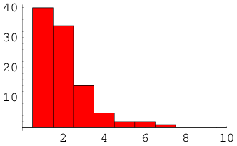
Figure 2: Distribution of $\sqrt{Q}/2=[{\rm vol}(T^{2})/\ell_{s}^{2}]_{\rm Het}$ in the miniature landscape (conditions (21, 28)) from F-theory on ${\rm K3}\times{\rm K3}$.

It is clear that only a small fraction of vacua in the tail of the distribution in Figure 2 are in the moduli space of K3 surfaces $X$ in the stable degeneration “limit”, or in the large ${\rm vol}(T^{2})/\ell_{s}^{2}$ region of heterotic $E_{8}\times E_{8}$ compactification.

This distribution can be regarded as that of an ensemble of effective theories containing $E_{8}\times E_{8}$ 7-brane gauge groups (which are left unbroken), but it can also be regarded as that of theories with $\mathop{\rm SO}(32)$ 7-brane gauge group.

For moderate choices of a, b and c, we should not expect that $\epsilon_{K}$ is small, either. In other words, all the period integrals in such a K3 surface either vanish or are of order unity. This means that there is no extra singular fibre located closely to a singular fibre supporting 7-brane non-Abelian gauge groups, like $H^{\rm v}$ and $H^{\rm h}$ in the visible and hidden sector. Correspondingly, the appropriate field theory local model is to take $H^{\rm v}$ and $H^{\rm h}$ as the gauge group everywhere on the other K3 surface $S$.

Let us now turn our attention back to the defining equation (86) of the K3 surface. Certainly it is a better and more direct approach for a systematic search for the Noether–Lefschetz locus of $Y$ to parametrize the moduli space by period integrals and deal with the lattices $T_{X}$, $S_{X}$ etc., but it is also nice if we can figure out what kind of defining equations such vacua correspond to. Precisely the same problem has been addressed by [85, 73] for a specific class of K3 surfaces. In the following, we provide a simplified summary of their results so it fits to the context in this article.

Consider an attractive K3 surface $X_{[2A~{}2B~{}2C]}$ (i.e., special case $a=2A$, $b=2B$ and $c=2C$). Such a K3 surface corresponds to ${\rm Km}(E_{\rho_{1}}\times E_{\rho_{2}})=(E_{\rho_{1}}\times E_{\rho_{2}})/\mathbb{Z}_{2}$ with

$$\rho_{1}=\frac{-B+i\sqrt{4AC-B^{2}}}{2C},\qquad\rho_{2}=\frac{-B+i\sqrt{4AC-B^{2}}}{2}=C\rho_{1}\,.$$ (97)

$E_{\rho_{i}}$ ($i=1,2$) is an elliptic curve with the complex structure $\rho_{i}$, and we let its defining equation be $y^{2}=x(x-1)(x-\lambda_{i})$. Kummer surfaces associated with a product type Abelian surface, which have $\rho_{X}=18$, are known to have at least 11 different types of elliptic fibrations [74]. One of them (type 3 in [74]) has $2{\rm IV}^{*}+8I_{1}$ type singular fibres (including two “$E_{6}$-type” fibres) in the Kodaira classification. Let us take this type of elliptic fibration as an example. Ref. [85] found that the Weierstrass model for this type of fibration (Inose’s pencil) is given by

$$Y^{2}=(X+4u^{2})(X+4u^{2}(\lambda_{1}+\lambda_{2}))(X+4u^{2}\lambda_{1}\lambda_{2})+\frac{(4u^{2})^{3}}{4}\left\{\frac{\lambda_{2}(\lambda_{2}-1)}{u}+\lambda_{1}(\lambda_{1}-1)u\right\}^{2}\,,$$ (99)

where $u$ is the inhomogeneous coordinate on the base $\mathbb{P}^{1}$, or equivalently,

$$\tilde{Y}\left\{\tilde{Y}-(2u)^{3}\left(\frac{\lambda_{2}(\lambda_{2}-1)}{u}+\lambda_{1}(\lambda_{1}-1)u\right)\right\}=(X+4u^{2})(X+4u^{2}(\lambda_{1}+\lambda_{2}))(X+4u^{2}\lambda_{1}\lambda_{2})\,.$$ (100)

Tate’s condition for a ${\rm IV}^{*}$ fibre is satisfied at $u=0$ and $u=\infty$. To turn this $\rho_{X}=18$ K3 surface into an attractive K3 surface ($\rho_{X}=20$), we only have to make a specific choice of $\rho_{1}$ and $\rho_{2}$ (and hence $\lambda_{1,2}$) in terms of integers $A$, $B$ and $C$ as in (97). The second equation above is already in the form of the generalized Weierstrass form (Tate form, (86)), apart from a shift in $X$ that does not play an essential role. The defining equation of the spectral surface can be read off from the Tate form: $a^{\rm v}_{0}=a^{\rm v}_{2}=0$, and $a^{\rm v}_{3}y=0$. Thus, in the language of the supergravity approximation of heterotic string theory, the $\rho_{X}=20$ vacua of F-theory are realized due to spectral surfaces (gauge field configurations) which are far from generic and imply an intricate conspiracy among $f_{0}$, $g_{0}$, $a^{\rm v}_{3}$ and $a^{\rm h}_{3}$. We will come back to this issue in Section 5.3 and Appendix B.

5 Landscapes of F-theory on ${\rm K3}\times{\rm K3}$ with $G_{0}\neq 0$ Flux

The study in the previous section is for a landscape with a limited choice of four-form flux; the condition (21) has been imposed. Consequently, the number of vacua is limited and the level of complexity of the analysis remains (barely) manageable. One can maintain full control of details, if one wishes, which enables us to understand various subtleties associated with multiplicity counting and the role played by the modular group. The $G_{0}=0$ assumption on the flux, however, has much to do with this advantage.

Suppose that $Y=X\times S$ for F-theory compactification is given by a pair of attractive K3 surfaces $X$ and $S$, as in Section 2.1. The $G_{0}$ type flux is then in $S_{X}\otimes S_{S}\otimes\mathbb{R}$ and can be written in the form

$$[G_{0}]=\sum_{I=1}^{18}C_{I}\otimes F_{I}\,,$$ (101)

where $\{C_{I}\}_{I=1,\cdots,18}$ is chosen as a basis of $W_{\rm root}\oplus W_{\rm{\rm U}(1)}\subset W_{\rm frame}\subset S_{X}$ and $F_{I}\in S_{S}\otimes\mathbb{Q}\subset H^{1,1}(S;\mathbb{R})$. The gauge bosons corresponding to the Cartan part of the 7-brane gauge fields remain massless for a rank-$rk_{7}$ group when the $\{F_{I}\}$s span an $(18-rk_{7})$-dimensional subspace of $H^{1,1}(S;\mathbb{R})$. The rest of the Cartan gauge fields become massive through the Stückelberg mechanism. There will be $(18-rk_{7})$ global ${\rm U}(1)$ symmetries left in the effective theory. Non-perturbative corrections break these symmetries, but they may still look like approximate symmetries if the non-perturbative corrections break them only weakly.

Therefore it is not a complete nonsense to focus on a sub-ensemble of vacua of F-theory on ${\rm K3}\times{\rm K3}$ with $G_{\rm tot}=G_{1}+G_{0}$ flux of a given value of $(18-rk_{7})$ and to study the statistics of this sub-ensemble, as those compactifications share a common property of the resulting effective theories. In this context, the statistical results of the $G_{0}=0$ landscape in Section 4.3 are also of some value. They are regarded as the statistics in the sub-ensemble characterized by the rank $rk_{7}=18$ massless gauge group on 7-branes and ${\cal N}=1$ supersymmetry.

There is hence a physical motivation to study the statistics of the sub-landscape characterized by some properties of the $G_{0}$ flux, such as $rk_{7}$ (see Sections 5.3 and 5.4 for more), and also to compare the numbers of vacua that have $G_{0}$ with different properties. These are the kind of problems we address in this section.

5.1 General Remarks

5.1.1 Primitivity

Let us begin with a brief remark on the Kähler moduli. For supersymmetric compactifications, $G_{\rm tot}=G_{1}+G_{0}$ not only has to be purely of Hodge type $(2,2)$, but also primitive:

$$J_{Y}\wedge G_{\rm tot}=J_{Y}\wedge G_{0}=0\,.$$ (102)

The Kähler form $J_{Y}$ on $Y=X\times S$ has the shape

$$J_{Y}=t_{X}[F_{X}]+J_{S}\,,$$ (103)

where $t_{X}\in\mathbb{R}_{0<}$, $[F_{X}]$ is the fibre class (elliptic divisor) associated with $\pi_{X}:X\rightarrow\mathbb{P}^{1}$, and $J_{S}$ a Kähler form on $S$ in the positive cone of $S_{S}$ (i.e., $J_{S}\in S_{S}\otimes\mathbb{R}$, and $J_{S}^{2}>0$). The primitivity condition (102) implies that all of the $F_{I}$ ($I=1,\cdots,18$) are orthogonal to $J_{S}$ in the inner product in $S_{S}\otimes\mathbb{R}\cong H^{1,1}(S;\mathbb{R})$. For a given Kähler form $J_{S}$, the $G_{0}$ type flux in $W_{{\rm frame}*}\otimes[J_{S}^{\perp}\subset(S_{S}\otimes\mathbb{R})]$ always gives rise to a positive contribution—$1/2[G_{0}]\cdot[G_{0}]$—to the D3-tadpole, since both $W_{\rm frame}$ and $[J_{S}^{\perp}\subset S_{S}\otimes\mathbb{R}]$ are negative definite.

Because of the primitivity condition of the four-form flux, the complex structure moduli and Kähler moduli talk to each other. There are two equivalent ways to see how they “talk”. One way is, to think of the Kähler moduli $(t_{X},J_{S})$ as being given first, after which the $F_{I}$ describing $G_{0}$ are forced to be in the subspace $[J_{S}^{\perp}\subset S_{S}\otimes\mathbb{Q}]$, as above. If the ratio of components of $J_{S}$ are in $\mathbb{Q}$—this situation is denoted by $[J_{S}]\in\mathbb{Q}\mathbb{P}[S_{S}]$ in this article—then $[J_{S}^{\perp}\subset S_{S}\otimes\mathbb{Q}]$ is of dimension [20-1=19]. If the ratio is not just in $\mathbb{Q}$, but in an extension field of $\mathbb{Q}$, then the dimension of the space for $G_{0}$ is smaller than 19. In the rest of this article, we assume that $J_{S}\in\mathbb{Q}\mathbb{P}[S_{S}]$. The other way is to think of the $F_{I}$ as being given first. In this case, $J_{S}$ is forced to be in the subspace of $S_{S}\otimes\mathbb{R}$ orthogonal to all of the $F_{I}$ due to the D-term potential (e.g., [13, 21]). When the $F_{I}$ span a $(18-rk_{7})$-dimensional subspace of $S_{S}\otimes\mathbb{Q}$, the remaining moduli space of $J_{S}$ is of $(2+rk_{7})$-dimensions (in $\mathbb{R}$)., Eventually one has to think of stabilization of both complex structure moduli and Kähler moduli, so that these two perspectives are equivalent. Common to these two is the idea that the stabilization of the two groups of moduli can be dealt with separately, which is true as long as there is a separation of scales between those two stabilization mechanisms, such as in the KKLT scenario [89].

In this article, we focus on aspects of complex structure moduli stabilization in flux compactifications, using ${\rm K3}\times{\rm K3}$ as an example. This article is not committed to a particular mechanism of Kähler moduli stabilization available on ${\rm K3}\times{\rm K3}$, except that we implicitly assume this separation of scales. It is thus impossible to determine the full landscape distribution of completely discrete vacua in the product of complex structure and Kähler moduli spaces ${\cal M}_{\rm cpx}\times{\cal M}_{\rm Kahler}$ for ${\rm K3}\times{\rm K3}$, or projections of these distributions to ${\cal M}_{\rm cpx}$, without introducing extra assumptions (on Kähler moduli stabilization). Our statements in the rest of this article are often presented in the form of distributions of flux vacua on ${\cal M}_{\rm cpx}$ for a fixed choice of Kähler moduli.

5.1.2 Integrality

Let us now switch the subject, and discuss the “integrality condition” on $[G_{1}]$ and $[G_{0}]$. When both $[G_{1}]$ and $[G_{0}]$ are non-zero, each one of them does not have to be integral by itself; only the total flux $[G_{\rm tot}]=[G_{1}]+[G_{0}]$ needs to be integral, i.e. an element of $H^{4}(Y;\mathbb{Z})$. Once we find that $[G_{1}]$ does not have to be integral—an element of $T_{X}\otimes T_{S}$—on its own, the condition (24) is too restrictive. Contributions to the D3-brane tadpole, $[G_{1}]\cdot[G_{1}]/2$ and $[G_{0}]\cdot[G_{0}]/2$, are not necessarily integers separately either, though their sum is always integral, when $G_{\rm tot}$ is integral. This means that the search for pairs of attractive K3 surface in Sections 2.1 and 2.2 needs to be carried out once again for cases with $G_{0}\neq 0$. How large is the impact of this generalization ?

In cases where both $X$ and $S$ are attractive K3 surfaces, we can decompose the $22\times 22$-dimensional vector space $H^{2}(X,\mathbb{R})\times H^{2}(S,\mathbb{R})$ into

$$[(T_{X}\otimes T_{S})\otimes\mathbb{R}]\,\oplus\,[(T_{X}\otimes S_{S})\otimes\mathbb{R}]\,\oplus\,[(S_{X}\otimes T_{S})\otimes\mathbb{R}]\,\oplus\,[(S_{X}\otimes S_{S})\otimes\mathbb{R}].$$ (104)

Such a decomposition is not necessarily possible with integer coefficients, not all of the elements of $H^{2}(X;\mathbb{Z})$ (resp. $H^{2}(S;\mathbb{Z})$) can be written in the form of a sum of integral elements in $T_{X}$ and $S_{X}$ (resp. $T_{S}$ and $S_{S}$), and not all the elements in $H^{2}(X,\mathbb{Z})\times H^{2}(S,\mathbb{Z})$ can be written as a sum of integral elements in

$$[(T_{X}\otimes T_{S})]\,\oplus\,[(T_{X}\otimes S_{S})]\,\oplus\,[(S_{X}\otimes T_{S})]\,\oplus\,[(S_{X}\otimes S_{S})].$$ (105)

The integrality of the total flux $[G]=[G_{1}]+[G_{0}]$, however, implies that for all the generators of $T_{X}\otimes T_{S}$ and $S_{X}\otimes S_{S}$, which are all integral four-cycles, the flux quanta evaluated on these cycles are integers. Hence $[G_{1}]$ and $[G_{0}]$ are contained within $(T_{X}\otimes T_{S})^{*}=(T_{X}^{*}\otimes T_{S}^{*})\subset(T_{X}\otimes T_{S})\otimes\mathbb{Q}$ and $(S_{X}\otimes S_{S})^{*}=(S_{X}^{*}\otimes S_{S}^{*})\subset(S_{X}\otimes S_{S})\otimes\mathbb{Q}$, respectively. In particular, it follows that $[G_{1}]$ should be within $T_{X}^{*}\otimes T_{S}^{*}$, but may not necessarily be within $T_{X}\otimes T_{S}$.

In fact, there is a stronger necessary condition than this; although the projection of $H^{2}(S;\mathbb{Z})\subset T_{S}^{*}\oplus S_{S}^{*}$ to $T_{S}^{*}$ for an attractive K3 surface is always surjective, the projection image of

$$(H^{2}(S_{1};\mathbb{Z})\otimes H^{2}(S_{2};\mathbb{Z}))\cap[H^{4,0}(Y;\mathbb{C})\oplus H^{2,2}(Y;\mathbb{R})\oplus H^{0,4}(Y;\mathbb{C})]$$ (106)

to $(T_{S_{1}}\otimes T_{S_{2}})^{*}$, for $Y=S_{1}\times S_{2}$ with a pair of attractive K3 surfaces $S_{1}$ and $S_{2}$, is not. In order to state a condition on the image of this projection, note that, for a pair of attractive K3 surfaces $S_{1}$ and $S_{2}$, the transcendental lattices, Neron–Severi lattices and their dual lattices have the following properties: as Abelian groups,

$$T_{S_{i}}^{*}/T_{S_{i}}\cong\mathbb{Z}_{m_{i}}\times\mathbb{Z}_{n_{i}},\qquad S_{S_{i}}^{*}/S_{S_{i}}\cong\mathbb{Z}_{m_{i}}\times\mathbb{Z}_{n_{i}},\qquad{}^{\exists}\gamma_{i}:T_{S_{i}}^{*}/T_{S_{i}}\cong S_{S_{i}}^{*}/S_{S_{i}}\qquad(i=1,2)$$ (107)

for some positive integers $m_{i},n_{i}$. It then follows that

$$(T_{S_{1}}\otimes T_{S_{2}})^{*}/(T_{S_{1}}\otimes T_{S_{2}})\cong\mathbb{Z}_{m_{1}m_{2}}\times\mathbb{Z}_{m_{1}n_{2}}\times\mathbb{Z}_{n_{1}m_{1}}\times\mathbb{Z}_{n_{1}n_{2}}\,.$$ (108)

One can prove that the image of the integral four-cycles in (106) has to be within the subgroup of $(T_{S_{1}}\otimes T_{S_{2}})^{*}$ characterized by

$${\rm LCD}(m_{1},m_{2})\mathbb{Z}_{m_{1}m_{2}}\times\cdots\times{\rm LCD}(n_{1},n_{2})\mathbb{Z}_{n_{1}n_{2}}\subset\mathbb{Z}_{m_{1}m_{2}}\times\cdots\times\mathbb{Z}_{n_{1}n_{2}}\,.$$ (109)

Because of this necessary condition on $[G_{1}]$, one can see that $[G_{1}]$ still has to be an integral element of $T_{X}\otimes T_{S}$ if all the four pairs $(m_{1},m_{2})$, $(m_{1},n_{2})$, $(n_{1},m_{2})$ and $(n_{1},n_{2})$ are mutually coprime. In this case, all the possible forms of the $[G_{1}]$ component on a pair of attractive K3 surfaces $X\times S=S_{1}\times S_{2}$ remain the same as in Sections 2.1 and 2.2. When the four pairs of integers are not coprime, however, there are more chances for the $[G_{1}]$ component available in the (sublattice of) the $(T_{X}\otimes T_{S})^{*}$ lattice than in the $T_{X}\otimes T_{S}$ lattice. That makes it easier to pass the D3-tadpole constraint (28), even for a pair of attractive K3 surfaces with relatively large values of $a,c$ and $d,f$. Section 5.2 is devoted to an explicit enumerative study in order to see more of the consequences of this possibility of non-integral choice of $G_{1}$.

5.1.3 $\left\langle{W_{\rm GVW}}\right\rangle=0$

When we write the $[G_{1}]$ component as $G_{1}={\rm Re}[\gamma\Omega_{S_{1}}\wedge\overline{\Omega}_{S_{2}}]$, as in [17] or in (25), it manifestly has only a $(2,2)$ Hodge component, without $(4,0)$ or $(0,4)$ component. However, we may also ask what is the statistical cost of requiring the absence of the $(4,0)+(0,4)$ components, or equivalently, a vanishingly small cosmological constant. For this purpose, the $G_{0}$ component is irrelevant and $[G_{1}]\in(T_{S_{1}}\otimes T_{S_{2}})\otimes\mathbb{Q}$, which we can write as:

$$[G_{1}]=k_{1}(p_{1}\otimes p_{2})+k_{2}(p_{1}\otimes q_{2})+k_{3}(q_{1}\otimes p_{2})+k_{4}(q_{1}\otimes q_{2})\,,$$ (110)

where $k_{1},k_{2},k_{3},k_{4}\in\mathbb{Q}$ are not necessarily integers. The $(4,0)$ and $(0,4)$ Hodge components of $[G_{1}]$ are

$$\frac{\bar{\tau}_{1}\bar{\tau}_{2}k_{1}-\bar{\tau}_{1}k_{2}-\bar{\tau}_{2}k_{3}+k_{4}}{(\bar{\tau}_{1}-\tau_{1})(\bar{\tau}_{2}-\tau_{2})}\;\Omega_{S_{1}}\wedge\Omega_{S_{2}}+\frac{\tau_{1}\tau_{2}k_{1}-\tau_{1}k_{2}-\tau_{2}k_{3}+k_{4}}{(\bar{\tau}_{1}-\tau_{1})(\bar{\tau}_{2}-\tau_{2})}\;\overline{\Omega}_{S_{1}}\wedge\overline{\Omega}_{S_{2}}\,.$$ (111)

Thus, the absence of the $(4,0)+(0,4)$ component is equivalent to the condition that either $(\tau_{1}\tau_{2})$, $\tau_{1}$, $\tau_{2}$ and $1$ are not linear independent over the field $\mathbb{Q}$, or all of $k_{1,2,3,4}$ vanish (and $G_{1}=0$). For an arbitrary pair of attractive K3 surfaces $S_{1}$ and $S_{2}$, the period integrals take their values in $\mathbb{Q}[\tau_{1},\tau_{2}]$, which is a degree ${\cal D}=4$ algebraic extension field over $\mathbb{Q}$. The condition for this pair $S_{1}$ and $S_{2}$ to admit a flux with vanishing cosmological constant (while $G_{1}\neq 0$), however, has turned out to be that $\tau_{2}$ is already contained in $\mathbb{Q}[\tau_{1}]$, and $\mathbb{Q}[\tau_{1},\tau_{2}]$ is a degree ${\cal D}=2$ extension field of $\mathbb{Q}$. The condition (26) is for $\left\langle{W}\right\rangle=0$, for a general non-vanishing $[G_{1}]$ in $(T_{X}\otimes T_{S})\otimes\mathbb{Q}$, rather than just for an integral $[G_{1}]\in(T_{X}\otimes T_{S})$.

5.2 A Landscape of Vacua with a Rank-16 7-brane Gauge Group

Just like the $G_{0}=0$ landscape in Section 4.3, which is interpreted as the ensemble of vacua with rank-18 massless gauge fields on 7-branes, let us also consider the ensemble of F-theory compactifications on ${\rm K3}\times{\rm K3}$ with rank-16 massless gauge fields on 7-branes. This is realized by allowing a $G_{0}\neq 0$ with only two terms non-zero in the expansion (101). With this study, we hope to elucidate various aspects of the landscape involving $G_{0}\neq 0$. In the context of F-theory, there is not particular importance to the specific choice of having just two terms in (101), or equivalently $rk_{7}=16$. However, this choice makes it easier to link the present discussion to earlier results on type IIB orientifold landscapes, as discussed in Section 5.4.

Suppose that $G_{0}\neq 0$ flux is introduced by using some $C_{I=1}$ and $C_{I=2}$ in (101), where $C_{I=1,2}$ are elements of the frame lattice $W_{\rm frame}(X_{[a~{}b~{}c]})$ of some attractive K3 surface $X_{[a~{}b~{}c]}$. Then the gauge fields along the direction of $C_{I=1,2}$ become massive, and only the gauge fields within $[\{C_{I=1,2}\}^{\perp}\subset W_{\rm frame}]$ remain massless. Since it is motivated from the perspective of physics to collect vacua with a given unbroken gauge group, it will be interesting to consider, for a given rank-$16=rk_{7}$ lattice $W_{\rm unbroken}$, the vacuum ensemble associated with

$$\left\{\left(W_{\rm frame},\{C_{I=1,2}\}\right)\;|\;W_{\rm frame}\in\amalg_{X_{[a~{}b~{}c]}\in{\rm Isom}(\Lambda_{\rm K3})\backslash D_{\rho=20}}{\cal J}_{2}(X_{[a~{}b~{}c]}),\right.$$ (112)

$$\qquad\qquad\qquad\qquad\qquad\qquad\left.\;C_{I=1,2}\in W_{\rm frame},\;[\{C_{1,2}\}^{\perp}\subset W_{\rm frame}]=W_{\rm unbroken}\right\}\,.$$

For this reason, it also makes sense to use the notation $W_{\rm noscan}$ instead of $W_{\rm unbroken}$. These two are used interchangeably in Section 5.2, but they are distinguished in Section 5.4.

If we are to take the rank-16 lattice to be e.g. $W_{\rm unbroken}=E_{8}\oplus E_{8}$ or $D_{16};\mathbb{Z}_{2}\left\langle{\bf sp}\right\rangle$, then for all the attractive K3 surfaces $X$, there is an embedding of the transcendental lattice $T_{X}$, the hyperbolic plane lattice $U_{*}\cong{\rm Span}_{\mathbb{Z}}\{[F_{X}],\sigma\}$ associated with elliptic fibration, and $W_{\rm unbroken}$ (which is an even unimodular lattice of signature $(0,16)$) into the cohomology lattice $\Lambda_{\rm K3}^{(X)}$:

$$U_{*}\oplus\left(T_{X}\oplus T_{X}[-1]\right)\oplus W_{\rm unbroken}\hookrightarrow U_{*}\oplus\left(U\oplus U\right)\oplus W_{\rm unbroken}\cong\Lambda_{\rm K3}^{(X)}\,.$$ (113)

The Neron–Severi lattice is $S_{X}\cong U_{*}\oplus T_{X}[-1]\oplus W_{\rm unbroken}$, and the frame lattice is $W_{\rm frame}\cong T_{X}[-1]\oplus W_{\rm unbroken}$. Hence we choose the generators of the rank-2 lattice $T_{X}[-1]=[W_{\rm unbroken}^{\perp}\subset W_{\rm frame}]$ as $\{C_{I=1,2}\}$ [15, 23].

As another example of $W_{\rm unbroken}$, one can also think of $(D_{4}\oplus D_{4}\oplus D_{4}\oplus D_{4});(\mathbb{Z}_{2}\times\mathbb{Z}_{2})$, in which case a type IIB orientifold interpretation is given. It is known that there is an embedding

$$\left(U[2]\oplus U[2]\right)\oplus(U_{*}\oplus W_{\rm unbroken})\hookrightarrow\Lambda_{\rm K3}^{(X)}\,.$$ (114)

Furthermore, it is known that for attractive K3 surfaces $X_{[a~{}b~{}c]}$ with $a,b,c$ even, there is an embedding $T_{X}\oplus T_{X}[-1]\hookrightarrow U[2]\oplus U[2]$ ([61, 59, 62, 17]). Thus, $W_{\rm frame}\cong T_{X}[-1]\oplus W_{\rm unbroken}$, and the generators of the rank-2 lattice $T_{X}[-1]=[W_{\rm unbroken}^{\perp}\subset W_{\rm frame}]$ are chosen as $\{C_{I=1,2}\}$s. [15, 23] Hence all the attractive K3 surfaces with even $a,b,c$ contribute to the ensemble of vacua characterized by $W_{\rm unbroken}\cong(D_{4}^{\oplus 4});(\mathbb{Z}_{2}\times\mathbb{Z}_{2})$.

Let $T_{S}$ be the transcendental lattice of the attractive K3 surface $S$. Modulo ${\rm Isom}(\Lambda_{\rm K3}^{(S)})$, it is always possible to embed $T_{S}$ into $\Lambda_{\rm K3}^{(S)}$ as

$$T_{S}\hookrightarrow(T_{S}\oplus T_{S}[-1])\hookrightarrow(U\oplus U)\oplus U\oplus E_{8}\oplus E_{8}\cong\Lambda_{\rm K3}^{(S)}\,.$$ (115)

This is not only always possible, but also unique in that any embedding to $\Lambda_{\rm K3}^{(S)}\cong{\rm II}_{3,19}$ (not to ${\rm II}_{2,18}$) can be brought in the form above modulo ${\rm Isom}(\Lambda_{\rm K3}^{(S)})$ [77]. Thus, $S_{S}\cong T_{S}[-1]\oplus U\oplus E_{8}\oplus E_{8}$. Therefore, the flux $G_{\rm tot}=G_{1}+G_{0}$ is introduced to the space

$$\left[(T_{X}\otimes T_{S})^{*}\oplus(T_{X}[-1]\otimes(T_{S}[-1]\oplus U\oplus E_{8}\oplus E_{8}))^{*}\right]\cap H^{2}(X;\mathbb{Z})\otimes H^{2}(S;\mathbb{Z})\,.$$ (116)

Now, let us take the case $W_{\rm unbroken}=E_{8}\oplus E_{8}$ as an example, and work out the details. In order to avoid inessential complexity, we restrict our attention to $Y=X\times S$ of the form $X_{[a~{}b~{}c]}\times X_{[a^{\prime}~{}b^{\prime}~{}c^{\prime}]}$ with $b=b^{\prime}=0$. Embeddings of (113, 115) are given by

$$(p_{1},P_{1},q_{1},Q_{1}) = (v_{1},V_{1},v^{\prime}_{1},V^{\prime}_{1})\left(\begin{array}[]{cccc}1&-1&&\\ a&a&&\\ &&1&-1\\ &&c&c\end{array}\right)\,,$$ (121)

$$(p_{2},P_{2},q_{2},Q_{2}) = (v_{2},V_{2},v^{\prime}_{2},V^{\prime}_{2})\left(\begin{array}[]{cccc}1&-1&&\\ a^{\prime}&a^{\prime}&&\\ &&1&-1\\ &&c^{\prime}&c^{\prime}\end{array}\right)\,,$$ (126)

where $\{p_{1},q_{1}\}$ (resp. $\{p_{2},q_{2}\}$) are generators of $T_{X}$ (resp. $T_{S}$), and $\{P_{1},Q_{1}\}$ (resp. $\{P_{2},Q_{2}\}$) are generators of $T_{X}[-1]$ (resp. $T_{S}[-1]$). The $(U\oplus U)$ sublattice of $\Lambda_{\rm K3}^{(X)}$ is generated by $\{v_{1},V_{1}\}$ and $\{v^{\prime}_{1},V^{\prime}_{1}\}$, and that of $\Lambda_{\rm K3}^{(S)}$ by $\{v_{2},V_{2}\}$ and $\{v^{\prime}_{2},V^{\prime}_{2}\}$. The intersection forms on the $U$s are given by $(v,v)=(V,V)=0$ and $(v,V)=(V,v)=1$.

It is now straightforward to enumerate the flux $G_{\rm tot}=G_{1}+G_{0}$ in (116), using the basis give above:

$$G_{1} = \frac{n_{11}{\rm GCD}(a,a^{\prime})+m_{11}}{2{\rm GCD}(a,a^{\prime})}(p_{1}\otimes p_{2})+\frac{n_{22}{\rm GCD}(c,c^{\prime})+m_{22}}{2{\rm GCD}(c,c^{\prime})}(q_{1}\otimes q_{2})$$ (127)

$$\quad+\frac{n_{12}{\rm GCD}(a,c^{\prime})+m_{12}}{2{\rm GCD}(a,c^{\prime})}(p_{1}\otimes q_{2})+\frac{n_{21}{\rm GCD}(c,a^{\prime})+m_{21}}{2{\rm GCD}(c,a^{\prime})}(q_{1}\otimes p_{2}),$$

$$G_{0} = \frac{n_{11}{\rm GCD}(a,a^{\prime})-m_{11}}{2{\rm GCD}(a,a^{\prime})}(P_{1}\otimes P_{2})+\frac{n_{22}{\rm GCD}(c,c^{\prime})-m_{22}}{2{\rm GCD}(c,c^{\prime})}(Q_{1}\otimes Q_{2})+(P_{1}\otimes F_{P})+(Q_{1}\otimes F_{Q})$$ (128)

$$\quad+\frac{n_{12}{\rm GCD}(a,c^{\prime})-m_{12}}{2{\rm GCD}(a,c^{\prime})}(P_{1}\otimes Q_{2})+\frac{n_{21}{\rm GCD}(c,a^{\prime})-m_{21}}{2{\rm GCD}(c,a^{\prime})}(Q_{1}\otimes P_{2}),$$

$$G_{\rm tot} = n_{11}(v_{1}\otimes v_{2}+aa^{\prime}V_{1}\otimes V_{2})+m_{11}\frac{a^{\prime}v_{1}\otimes V_{2}+aV_{1}\otimes v_{2}}{{\rm GCD}(a,a^{\prime})}+\cdots+(P_{1}\otimes F_{P})+(Q_{1}\otimes F_{Q})\,.$$ (129)

Here, $n_{11},m_{11},\cdots,n_{22},m_{22}$ are integers and $F_{P},F_{Q}\in U\oplus E_{8}\oplus E_{8}\subset\Lambda_{\rm K3}^{(S)}$. The denominators ${\rm GCD}(2a,2a^{\prime})$, ${\rm GCD}(2c,2c^{\prime})$ etc. in (127, 128) correspond to our earlier discussion around (109). $G_{1}$ and $G_{0}$ are not necessarily integral separately, but $G_{\rm tot}$ is. At this moment, it is not guaranteed that the $(4,0)+(0,4)$ Hodge components vanish. After imposing the $\left\langle{W}\right\rangle=0$ condition, one is left with the following cases

• ${\cal D}:=\dim_{\mathbb{Q}}\mathbb{Q}[\tau_{1},\tau_{2}]=2$, i.e., the condition (26) is satisfied when $G_{1}\neq 0$ and there are $(8-{\cal D})=6$ independent integers out of $\{n_{11},\cdots,m_{22}\}$, in addition to $F_{P},F_{Q}$. In this case there are ${\cal D}=2$ less scanning integers just like in Sections 2.1, 2.2 and [17].

• ${\cal D}=4$, when $G_{1}=0$, and there are $(8-{\cal D})=4$ independent integers as well as $F_{P},F_{Q}$ (the “second branch” in §5 of [21]).

The latter ii) cases leave 16 moduli of $X$ and 18 of $S$ unstabilized, and we restrict our attention only to the cases i) ,as [17] did, in the following.

Note, however, that the Kähler form and the primitivity condition on the flux has been ignored completely in the argument above. The Kähler form $J_{S}$ on $S$ needs to be introduced in the positive definite part of $[T_{S}^{\perp}\subset\Lambda_{\rm K3}]\otimes\mathbb{R}$, and the flux $G_{0}$ component has to be orthogonal to this $J_{S}$. We provide the following presentation for a fixed choice of $J_{S}$ (rather than scanning over all possible $J_{S}$), and in particular, we choose

$$J_{S}=t_{S}(v^{\prime\prime}_{2}+V^{\prime\prime}_{2})\,,$$ (130)

where $v^{\prime\prime}_{2}$ and $V^{\prime\prime}_{2}$ are the generators of the third copy of the hyperbolic plane lattice $U$ in $\Lambda_{\rm K3}^{(S)}$ in (115), so that the computation becomes as easy as possible. This means that the primitivity condition does not impose a constraint on the integers $\{n_{11},\cdots,m_{22}\}$, and $F_{P},F_{Q}$ are chosen from the negative definite lattice $(-2)\oplus E_{8}\oplus E_{8}$. Here, $(-2)$ is the lattice generated by $(v^{\prime\prime}_{2}-V^{\prime\prime}_{2})$, where $(v^{\prime\prime}_{2}-V^{\prime\prime}_{2})^{2}=-2$.

Assuming that $W_{\rm unbroken}=E_{8}\oplus E_{8}$ (or $D_{16};\mathbb{Z}_{2}\left\langle{\bf sp}\right\rangle$), we scan all possible pairs of attractive K3 surfaces of the form $X_{[a~{}0~{}c]}\times X_{[a^{\prime}~{}0~{}c^{\prime}]}$ and list up all the possible fluxes (127, 128) satisfying (i) the condition that $\left\langle{W}\right\rangle=0$, (ii) the primitivity condition with respect to the Kähler form (130) and (iii) the D3-tadpole condition

$$\frac{1}{2}G_{\rm tot}\cdot G_{\rm tot}\leq\frac{\chi(X\times S)}{24}=24\,;$$ (131)

the remaining D3-brane charge is supplied by placing an appropriate number of D3-branes.

Scanning within the range of $0<c\leq a\leq 50$ and $0<c^{\prime}\leq a^{\prime}\leq 50$ for $Y=X\times S=X_{[a~{}0~{}c]}\times X_{[a^{\prime}~{}0~{}c^{\prime}]}$, we found that there are 313 different choices of $X\times S$ admitting the flux satisfying all the three conditions above. The distribution of the value of $a$ in these 313 choices are shown in Figure 3. If both $G_{1}$ and $G_{0}$ were required to be integral, there would only be 28 different choices, and the largest possible value of $a$ would be 6.

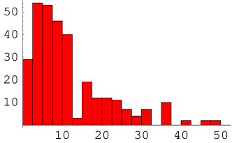
Figure 3: Variety in the choice of pairs of attractive K3 surfaces, $X\times S=X_{[a~{}0~{}c]}\times X_{[a^{\prime}~{}0~{}c^{\prime}]}$ is shown in the form of histograms of $a\leq 50$. This distribution is not weighted by the number of flux choices available.

Figure 4 shows the correlation among moduli parameters for the 313 pairs of attractive K3 surfaces admitting a flux satisfying all the three conditions above. For the first two scatter plots (i) and (ii) of Figure 4, we can see clear correlations. When $a$ is very large, there is presumably not much freedom to choose $a^{\prime}$ other than setting it to be comparable to $a$ itself (see (ii)), so that ${\rm GCD}(a,a^{\prime})$ is large, and the D3-tadpole contribution remains below the bound. On the other hand, there is no clear correlation to be read out from the plot (iii), we will have a comment on this in Section 5.4.

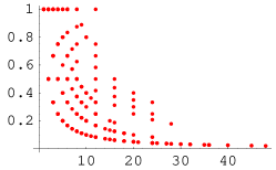
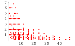
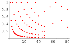
(i) $a$ vs $c/a$	(ii) $a$ vs $a^{\prime}/a$	(iii) $ac$ vs $c/a$

Figure 4: Scatter plots showing correlation between various modulus parameters $X$ (horizontal axis) vs $Y$ (vertical axis) for the 313 pairs of attractive K3 surfaces $X\times S=X_{[a~{}0~{}c]}\times X_{[a^{\prime}~{}0~{}c^{\prime}]}$. No weight proportional to the number of flux choices is included. (the blank region in the lower right corner of (iii) is an artefact of cutting the scan at $a,a^{\prime}\leq 50$)

There is a tremendous amount of combined choices of $X\times S=X_{[a~{}0~{}c]}\times X_{[a^{\prime}~{}0~{}c^{\prime}]}$ and the fluxes on it. We found about $795\times 10^{15}$ choices satisfying all the three conditions on the flux by naively scanning $\{n_{ij},m_{ij},F_{P},F_{Q}\}$ (apart from identification $\{n_{ij},m_{ij},F_{P},F_{Q}\}\longleftrightarrow(-1)\times\{n_{ij},m_{ij},F_{P},F_{Q}\}$). This large ensemble is dominated by the flux choices on a very small group of possibilities of $X_{[a~{}0~{}c]}\times X_{[a^{\prime}~{}0~{}c^{\prime}]}$. There are about $777\times 10^{15}$ choices of flux for $X_{[1~{}0~{}1]}\times X_{[1~{}0~{}1]}$, 98% of the ensemble. Almost 99.6% of the ensemble is accounted for when we combine all the flux choices on $X_{[1~{}0~{}1]}\times X_{[1~{}0~{}1]}$, $X_{[2~{}0~{}1]}\times X_{[2~{}0~{}1]}$, $X_{[2~{}0~{}2]}\times X_{[1~{}0~{}1]}$, $X_{[1~{}0~{}1]}\times X_{[2~{}0~{}2]}$ and $X_{[2~{}0~{}2]}\times X_{[2~{}0~{}2]}$.

It is a fluke, though, that the statistics is dominated by a small number of pairs of attractive K3 surfaces. The large number of flux choices for $X_{[a~{}0~{}c]}\times X_{[a^{\prime}~{}0~{}c^{\prime}]}$ with small values of $a,c,a^{\prime},c^{\prime}$ is primarily due to $F_{P},F_{Q}$ in $(-2)\oplus E_{8}\oplus E_{8}\subset\Lambda_{\rm K3}^{(S)}$. It is possible for such pairs of K3 surfaces to find a flux $(G_{1}+G_{0})$ on $(T_{X}\oplus T_{X}[-1])\otimes(T_{S}\oplus T_{S}[-1])$ so that the contribution to the D3-tadpole is much smaller than 24. There is a lot of room left in the tadpole condition for an extra $G_{0}$-type flux in $T_{X}[-1]\otimes((-2)\oplus E_{8}\oplus E_{8})$. It should be remembered that we should take a quotient of flux configurations on $X\times S=X_{[a~{}0~{}c]}\times X_{[a^{\prime}~{}0~{}c^{\prime}]}$ (and elliptic fibration morphisms) by the subgroup of $\Gamma$ that fixes the embeddings of $U_{*}\oplus T_{X}$ and $T_{S}$ in (113, 115) and $J_{S}$ in (130). Included in this stabilizer subgroup is $W_{E_{8}}\times W_{E_{8}}$, the Weyl group of $E_{8}\oplus E_{8}\subset\Lambda_{\rm K3}^{(S)}$.

The Weyl group $W_{E_{8}}$ acts on the 240 roots transitively. We have also confirmed that the norm $(-4)$, $(-6)$, $(-10)$ and $(-12)$ points form single orbits of $W_{E_{8}}$ on their own. There are at most two $W_{E_{8}}$ orbits in the norm $(-8)$ points, norm $(-14)$ points and also in the norm $(-16)$ points. Thus, it is not a particularly bad estimate (for the counting of inequivalent flux vacuum) to assume that all the norm $(-2m)$ points in the $E_{8}$ root lattice form a single orbit of $W_{E_{8}}$ for relatively small $m$ such as $m\leq 12$, which is the range that matters under the tadpole condition (131). With this crude approximation of the modular group $\Gamma$ action on fluxes, the total number of “inequivalent” choices of $X\times S=X_{[a~{}0~{}c]}\times X_{[a^{\prime}~{}0~{}c^{\prime}]}$ and fluxes $G_{\rm tot}$ combined is reduced to about $7\times 10^{6}$. About 80% of this ensemble of “inequivalent” vacua still come from fluxes on $X\times S=X_{[1~{}0~{}1]}\times X_{[1~{}0~{}1]}$, and the totality of the flux choices on the five $X\times S$ mentioned above (those with small $a,c,a^{\prime},c^{\prime}$) account for 92%. Although the precise percentage values should not be taken too seriously because of the crude estimate of the modular group action (and artificial choice of $J_{S}$), it is trustable at the qualitative level that the vacuum statistics of ${\rm K3}\times{\rm K3}$ compactifications of F-theory with a $rk_{7}=16$ 7-brane gauge group $W_{\rm unbroken}$ is dominated by a small number of $X\times S=X_{[a~{}b~{}c]}\times X_{[a^{\prime}~{}b^{\prime}~{}c^{\prime}]}$ which have small values of $a,c,a^{\prime},c^{\prime}$ so that the minimum possible value of $G_{\rm tot}^{2}/2$ is small. Consequently, the distribution of any observables/moduli parameters (such as ${\rm Im}(\rho_{H})=\sqrt{ac}$) is determined simply by that of $X\times S=X_{[1~{}0~{}1]}\times X_{[1~{}0~{}1]}$ and a few others.

Before closing this section, it is worthwhile to mention that non-zero flux $G_{\rm tot}=G_{1}+G_{0}$ does not imply that all the 18 + 20 complex structure moduli in ${\cal M}_{{\rm K3};F}^{(X)}\times{\cal M}_{{\rm K3}}^{(S)}$ are stabilized. The mass matrix (quadratic part of the superpotential) can be written in the form of

$$\propto\frac{1}{2}\left(\delta\Pi^{(1)},\delta\Pi^{(2)}\right)\left(\begin{array}[]{cc}-{\rm Im}(\tau_{2})\sqrt{Q_{2}}\gamma&\left.C_{I}\right)\otimes\left(F_{I}\right.\\ \left.F_{I}\right)\otimes\left(C_{I}\right.&-{\rm Im}(\tau_{1})\sqrt{Q_{1}}\overline{\gamma}\end{array}\right)\left(\begin{array}[]{c}\delta\Pi^{(1)}\\ \delta\Pi^{(2)}\end{array}\right)\,,$$ (132)

where $\delta\Pi^{(X)}$ has 18 components on $W_{\rm frame}$ and $\delta\Pi^{(S)}$ 20 components on $S_{S}$. Mass terms in the diagonal block are from (84), while the off-diagonal block is due to the $G_{0}$ type flux. All the moduli would have non-zero masses if $G_{1}\neq 0$ and $G_{0}$ were absent (and similarly, full rank $G_{0}$ type flux with $rk_{7}=0$ and vanishing $G_{1}$ would stabilize all but two complex structure moduli). When both are present, however, the diagonal masses from $G_{1}$ and off-diagonal masses from $G_{0}$ interfere and there may be a zero mass-eigenvalue (and an unstabilized direction of the moduli space) in principle.

One example is to choose $n_{ij}=0$, $m_{11}=m_{12}=m_{22}=-m_{21}=1$ and $F_{P}=F_{Q}=0$ in (127, 128) for a series of infinite pairs of attractive K3 surfaces $X\times S=X_{[k~{}0~{}k]}\times X_{[k~{}0~{}k]}$ (where $k=1,2\cdots,\infty$). Under this choice of the flux, a one parameter ($k$) deformation of the complex structure $\Omega_{X}\wedge\Omega_{S}=[(v_{1}+kV_{1})+i(v^{\prime}_{1}+kV^{\prime}_{1})]\otimes[(v_{2}+kV_{2})+i(v^{\prime}_{2}+kV^{\prime}_{2})]$ remains a flat direction, and all the $\rho_{X}=\rho_{S}=20$ points $X_{[k~{}0~{}k]}\times X_{[k~{}0~{}k]}$ just sit in this flat direction.

Such flux vacua with an unstabilized direction have been removed from the vacuum ensemble studied in this section. To be more precise, our numerical code examined the $4\times 4$ mass matrix on $P_{1}\delta\Pi^{(1)}_{P_{1}}+Q_{1}\delta\Pi^{(1)}_{Q_{1}}$ and $P_{2}\delta\Pi^{(2)}_{P_{2}}+Q_{2}\delta\Pi^{(2)}_{Q_{2}}$, and threw away all the flux configurations for which there is a zero eigenvalue in this mass matrix. Certainly, one should examine the eigenvalues of a $(18+20)\times(18+20)$ mass matrix for each flux configuration, but we believe that our short-cut approach does not qualitatively distort the distribution of observables in the landscape.

5.3 ${\rm U}(1)$ Flux, Heterotic–F-theory Duality, and GUT 7-brane Flux

The unbroken symmetry $W_{\rm unbroken}$ of interest for a sub-ensemble of vacua can be chosen at one’s will. We can choose it to be rank-18 as in Sections 2.1, 2.2 and 4.3, or to be rank-16 as in Section 5.2, but other choices such as $W_{\rm unbroken}\cong A_{4}$, a $\mathop{\rm SU}(5)_{\rm GUT}$ landscape, are just as appropriate.

Studies such as the one in Section 5.2 are dedicated to a landscape of vacua of individual choices of $W_{\rm unbroken}$, which we call the $W_{\rm unbroken}$ landscape. Beyond such an analysis, however, it is natural to ask such questions as how properties of the algebraic information $W_{\rm unbroken}$ generally characterize distributions within the $W_{\rm unbroken}$-landscape, or how the number of vacua in the $W_{\rm unbroken}$-landscape depends on $W_{\rm unbroken}$. As a preparation for such a discussion in Section 5.4, we make a few remarks in this Section.

When we write down the $G_{0}$ type flux in the form (101), we can take the generators $\{C_{I}\}_{I=1,\cdots,18}$ of $W_{{\rm frame}*}$ to be such that some are from $W_{{\rm U}(1)}$, and others from $W_{\rm root}$. We call the $G_{0}$ flux with $C_{I}$ from $W_{\rm U(1)}$ a ${\rm U}(1)$ flux or Mordell–Weil flux, and that with $C_{I}$ from $W_{\rm root}$ a GUT-brane flux or singular fibre flux. The GUT 7-brane flux corresponds to the line bundles introduced on GUT 7-branes in F-theory (such as those in [93]), or line bundles on a stack of multiple D7-branes in type IIB Calabi–Yau orientifolds. The ${\rm U}(1)$ flux requires [19] a special choice of complex structure so that there is a non-vertical algebraic cycle, meaning that the Mordell–Weil group is non-trivial; the unavoidable tuning of complex structure is an expression equivalent to moduli stabilization.

5.3.1 ${\rm U}(1)$ flux/Mordell–Weil flux

Let us first ask what the ${\rm U}(1)$ flux looks like in the light of the duality between F-theory and heterotic string theory. As discussed in the literature (such as [31, 32, 33]), there must be a component of four-form ${\rm U}(1)$ flux in F-theory whose origin in heterotic string is a flux on the spectral surface. Suppose that $\pi_{Z}:Z=T^{2}\times S\longrightarrow S$ is the elliptically fibred Calabi–Yau threefold for the dual heterotic string compactification, and $(C,{\cal N})$ the spectral data describing the vector bundle on $Z$. The spectral surface $C$ is a subspace of $Z={\rm Jac}(T^{2})\times S$ characterized by the zero points of the elliptic functions

$$a^{\rm v}_{0}+a^{\rm v}_{2}x+a^{\rm v}_{3}y+\cdots=0,\qquad a^{\rm h}_{0}+a^{\rm h}_{2}x+\cdots=0$$ (133)

on $T^{2}$, and ${\cal N}={\cal O}_{C}(\gamma)$ is a line bundle on $C$ specified by a divisor $\gamma$ on $C$. For any complex structure of $Z$, $S$ and $C$ [29], one can always find a divisor

$$\gamma_{\rm FMW}\propto(n\sigma-\pi_{C}^{*}(nK_{S}+\eta))\,,$$ (134)

where $\pi_{C}=\pi_{Z}|_{C}$, $\eta$ is a divisor on $S$, $K_{S}$ the canonical divisor of $S$, and we assume $\mathop{\rm SU}(n)\subset E_{8}^{\rm vis}$ is the structure group of the vector bundle. None of the ${\rm U}(1)$ fluxes we talk about here, however, should correspond to this Friedman–Morgan–Witten flux in the heterotic “dual”. If this flux were to be dual to the ${\rm U}(1)$ flux in F-theory, we would run into a contradiction immediately: an arbitrary complex structure is allowed on the heterotic side, while it has to be tuned in F-theory. In fact, the generic Friedman–Morgan–Witten flux (134) always vanishes, $\gamma=0$, when the dual F-theory is a ${\rm K3}\times{\rm K3}$ compactification.

For finely tuned complex structure of the heterotic string compactification data, $(Z,S,C)$, however, there is more variety in the choice of $\gamma$ on the spectral surface [29]. Suppose that the base K3 surface $S$ is not the general complex analytic one, but has Picard number $\rho_{S}\geq 2$. This means that we might be able to find a set of $\{F_{A}\}\subset[J_{S}^{\perp}\subset S_{S}]$ generating a rank-$k$ sublattice of $S_{S}$. We only consider vector bundles with the structure group contained in $G^{\rm v}_{\rm str}\times G^{\rm h}_{\rm str}=\mathop{\rm SU}(N_{v})\times\mathop{\rm SU}(N_{h})$. It then appears that we can think of a vector bundle for compactification,

$$V=\oplus_{i=1}^{N_{v}+N_{h}}{\cal O}_{S}(D_{i})\otimes{\cal O}_{T^{2}}(p_{i}-e),\qquad\qquad D_{i}=\sum_{A}n^{A}_{(i)}F_{A}\,,$$ (135)

where the $\{p_{i}\}$ and $e$ are the zeros and the pole, respectively, of the elliptic functions (133). The spectral surface is of the form $C=\cup_{i}C_{p_{i}}$ with $C_{p_{i}}\simeq S$’s corresponding to $p_{i}\in{\rm Jac}(T^{2})$, and $\gamma|_{C_{p_{i}}}=D_{i}$. This vector bundle is poly-stable with respect to the Kähler form $J_{Z}=J_{T^{2}}+J_{S}$. The unbroken symmetry should be $E_{9-N_{v}}^{\rm v}\times E_{9-N_{h}}^{\rm h}$ within $E_{8}\times E_{8}$. Moduli parameters include $\rho_{H}$ and $\tau_{H}$ of $T^{2}$, and $(N_{v}-1)+(N_{h}-1)$ parameters of the flat bundles in (133), and hence,in addition to those from the base $S$, there are $N_{v}+N_{h}$ of them.

Dual to this heterotic string compactification should be F-theory on $Y=X\times S$ where the elliptically fibred K3 surface $X$ has the following Neron–Severi and transcendental lattices:

$$\Lambda_{\rm K3}^{(X)}\supset S_{X}\oplus T_{X}=\left[U_{*}\oplus E_{9-N_{v}}\oplus E_{9-N_{h}}\right]\oplus\left[U\oplus U\oplus A_{N_{v}-1}\oplus A_{N_{h}-1}\right]\,.$$ (136)

K3 surfaces $X$ of this form have Picard number $\rho_{X}=(20-N_{v}-N_{h})$, so that the moduli space has dimension $(N_{v}+N_{h})$, which agrees with the counting above. If we are to find a four-form flux in F-theory dual to $\gamma$, that dual flux must be associated with non-$U_{*}$ cycles that are orthogonal to the unbroken symmetry part $E_{9-N_{v}}\oplus E_{9-N_{h}}$. This means that the flux is not in an algebraic cycle, and such a configuration is not stable. The complex structure moduli dynamically tune themselves (due to the GVW potential) so that the associated cycle becomes algebraic. In order to introduce $k$ independent ${\rm U}(1)$ fluxes in (101), the number of unstabilized directions in the moduli space should be reduced by $k$, and the moduli space becomes $(N_{v}+N_{h}-k)$-dimensional [19].

This reduction of the moduli space should also be understandable in the heterotic string description. Certainly $V$ in (135) is a holomorphic vector bundle and satisfies the condition $\int J\wedge J\wedge F=0$ as well as the Bianchi identity of the $B$-field,

$$0=\mathop{\rm tr}_{\mathfrak{so}(6)}\left[\left(\frac{R}{2\pi}\right)^{2}\right]-T_{R}^{-1}\mathop{\rm tr}{}_{R}\left[\left(\frac{F}{2\pi}\right)^{2}\right]+4\delta^{(4)}_{M5}=4\left(-c_{2}(TZ)-{\rm ch}_{2}(V)+\delta^{(4)}_{M5}\right)\,,$$ (137)

where $\delta^{(4)}_{M5}$ is the delta-function valued four-form associated with individual M5-branes wrapped on holomorphic curves in $Z=T^{2}\times S$, and ${\rm ch}_{2}(V)$ is the second Chern character of the rank $(N_{v}+N_{h})$ vector bundle $V$ (with the structure group $\mathop{\rm SU}(N_{v})\times\mathop{\rm SU}(N_{h})$). There is a condition that is stronger than (137), however:

$$0=H:=dB+\frac{\alpha^{\prime}}{4}\left(\mathop{\rm tr}\left[\omega d\omega+\frac{2}{3}\omega\omega\omega\right]-T_{R}^{-1}{\rm tr}{}_{R}\left[AdA-i\frac{2}{3}AAA\right]\right)+({\rm source})_{M5}\,,$$ (138)

if we are to stick to the framework of heterotic string compactification on a Kähler manifold and constant dilation configuration (Chap.16, [94]). This constraint may also be understood as a combination of the F-term condition of

$$W_{\rm Het}\propto\int_{Z}\Omega_{Z}\wedge H+(2\pi)^{2}\alpha^{\prime}\int_{\Gamma(M5)}\Omega_{Z}$$ (139)

with respect to the complex structure moduli of $Z$ and $\left\langle{W_{\rm Het}}\right\rangle=0$ for vanishing cosmological constant. $\Gamma(M5)$ is a real 3-chain in $Z=T^{2}\times{\rm K3}$ whose boundary contains the curves on which M5-branes are wrapped [95]. The exterior derivative of this condition (138) reproduces (137).

The $B$-field Bianchi identity, (137), can be satisfied by wrapping an appropriate number ($N_{M5}$) of heterotic NS5-branes (M5-branes in heterotic M-theory) on the fibre $T^{2}$. As is well-known in the literature,

$$c_{2}(TZ)=(24\;{\rm pt}_{K3})\otimes 1_{T^{2}},\qquad{\rm ch}_{2}(V)=\frac{1}{2}\sum_{i=1}^{N_{v}+N_{h}}(D_{i})^{2}\,,$$ (140)

and the only non-trivial part, which is a four-form on $S$ and scalar on $T^{2}$, of the condition (137) gives rise to

$$\frac{1}{2}(G^{(4)}_{H})^{2}+N_{M5}=24\,.$$ (141)

Here, $G^{(4)}_{H}$ takes values in the lattice $(A_{N_{v}-1}\oplus A_{N_{h}-1})\otimes[J_{S}^{\perp}\subset S_{S}]$, and is given by

$$G^{(4)}_{H}=\sum_{I=1}^{N_{v}-1}C_{I}\otimes D_{I}+\sum_{I=1}^{N_{h}-1}C_{I}\otimes D_{I},\qquad D_{I}=-(D_{i=1}+\cdots+D_{i=I})\,.$$ (142)

The condition (138) in the two-form component on $S$ and one-form on $T^{2}$, however, contains information that is not captured by the Bianchi identity (137). In the presence of ${\rm U}(1)$ flux ${\cal O}_{S}(D_{i})$ on $S$ and a flat bundle ${\cal O}_{T^{2}}(p_{i}-e)$ (i.e., Wilson line) on $T^{2}$, there is no contribution to the Chern character, but the Chern–Simons form can be non-zero. Keeping in mind that M5-branes wrapped on $T^{2}$ as well as gravitational Chern–Simons form only contribute to (138) in the component purely three-form on $S$, we see that

$$\left.\left(dB-\frac{\alpha^{\prime}}{4}T_{R}^{-1}\mathop{\rm tr}{}_{R}\left[AdA\right]\right)\right|_{2\mbox{-}{\rm form~{}on~{}}S,\;1\mbox{-}{\rm form~{}on~{}}T^{2}}=0\,,$$ (143)

where the $A^{3}$ term in the Chern–Simons form has also been dropped for the Cartan flux configuration. Since the Polyakov action remains invariant by changing the $B$-field background by $(2\pi)^{2}\alpha^{\prime}$ times an integral two-form on the target space, it is possible that the $B$-field background configuration expanded by using the same set of $F_{A}$ as in (135)

$$B=\sum_{A}b_{A}F_{A}(2\pi)^{2}\alpha^{\prime}$$ (144)

may have scalars $b_{A}$ varying topologically on $T^{2}$, so that $db_{A}=\check{\alpha}n^{8}_{A}+\check{\beta}n_{A}^{9}$ for some integers $n^{8}_{A}$ and $n^{9}_{A}$ and a basis $\{\check{\alpha},\check{\beta}\}$ of $H^{1}(T^{2};\mathbb{Z})$. When $k$ independent $F_{A}$’s in $[J_{S}^{\perp}\subset S_{S}]$ are involved, we find the $k$ independent conditions on the Wilson lines $A=A_{I}C_{I}$, $A_{I}=(2\pi)(\check{\alpha}a_{I}^{8}+\check{\beta}a_{I}^{9})$:

$$\left[db_{A}+\frac{A_{I}}{2\pi}\left(C_{I},C_{J}\right)n_{A}^{(J)}\right]\otimes F_{A}=0,\qquad 2n_{A}^{8}-a_{I}^{8}q^{I}_{A}=0,\quad 2n_{A}^{9}-a_{I}^{9}q^{I}_{A}=0,$$ (145)

where $n_{A}^{(J)}:=-(n^{A}_{(i=1)}+\cdots+n^{A}_{(i=J)})$ and $q^{I}_{A}:=-(C_{IJ})n_{A}^{(J)}$. Hence $k$ combinations of the Wilson lines $A_{I}$ are required to be torsion points of ${\rm Jac}(T^{2})$ (equivalent to the origin of ${\rm Jac}(T^{2})$ when multiplied by some non-zero integer). This is equivalent to $k$ conditions imposed on the spectral surface data ($a^{\rm v}_{0,2,3,\cdots}$ and $a^{\rm h}_{0,2,\cdots}$) and $f_{0}$ and $g_{0}$ (equivalently $\tau_{H}$).

Let us now translate this interplay among the Cartan flux, $B$-field topological configuration and the reduction (stabilization) of the moduli space in the language of Narain moduli. The Narain moduli covers not just the region with parametrically large $[{\rm vol}(T^{2})/\ell_{s}^{2}]$ (where supergravity approximation is good), but also the stringy region. When there is a Cartan flux and corresponding topological $dB$ configuration, our observation above—some combinations of $A_{I}$’s are forced to be torsions of ${\rm Jac}(T^{2})$—is translated into the existence of $k$ vectors

$$n_{A}:=(2n^{8}_{A},0,2n^{9}_{A},0,q^{I}_{A})^{T}\in{\rm II}_{2,18}\,,$$ (146)

satisfying

$$\langle{\cal Z}^{R},n_{A}\rangle=0,\qquad{\cal Z}^{R}\propto\left(-\tau_{H},\;-\tilde{\rho}_{H},\;1,\;-\tau_{H}\tilde{\rho}_{H}-(a)^{2}/2,\;a_{I}\right);$$ (147)

see Appendix A for background material on Narain moduli in heterotic string theory. This mechanism is precisely the same, mathematically, as how algebraic cycles emerge for special choice of complex structure on the other side of the duality.

It must be be obvious that one should define a lattice element

$$\widetilde{G}^{(4)}_{H}:=\sum_{A}n_{A}\otimes F_{A}\in[U\oplus U\oplus A_{N_{v}-1}\oplus A_{N_{h}-1}]\otimes[J_{S}^{\perp}\subset S_{S}]$$ (148)

in heterotic string language in order to formulate the Cartan flux and topological $dB$ configuration combined. Within the framework that we have assumed in this section so far, where $Z=T^{2}\times S$ is Kähler, $\left\langle{\phi}\right\rangle_{\rm Het}={\rm const}$ and $\left\langle{H}\right\rangle=0$ on the heterotic side, the duality map of the flux is given by

$$\widetilde{G}^{(4)}_{H}=G_{0}=G_{\rm tot}\,.$$ (149)

Within this class of Cartan flux, the norm of $\widetilde{G}^{(4)}_{H}$ remains the same as that of $G^{(4)}_{H}$, because with $w^{8}=w^{9}=0$, only $n_{8}^{A}$ and $n_{9}^{A}$ are allowed to be non-zero. Therefore, the Bianchi identity (141) becomes dual to the D3-tadpole condition (131).

The duality dictionary above is a generalization and refinement of the preceding discussion in [29, 96, 31, 97, 32, 33], in that we can deal with a more general class of fluxes on the heterotic spectral surface (by allowing non-trivial $\left\langle{dB}\right\rangle$), keep track also of flux quanta in the $U\oplus U$ components in the form of $\widetilde{G}^{(4)}_{H}=G_{\rm tot}$ or $n_{A}$, maintain a clear distinction between algebraic and transcendental cycles on the F-theory side and are able to understand how the dimension of moduli space is reduced.

The conventional dictionary using the stable degeneration limit of K3 surfaces is understood in the following way from the present perspective. Within the framework we have considered so far, the moduli space of ${\cal Z}^{R}$ ($\propto\Omega_{X}$) still maintains a free choice of at least $\tau_{H}$ and $\tilde{\rho}_{H}$, even after maximally possible Cartan fluxes (rank = $N_{v}+N_{h}-2$) are introduced in the $\mathop{\rm SU}(N_{v})\times\mathop{\rm SU}(N_{h})$ structure group (no $G_{1}$ component yet, in particular). Thus, from this moduli space we can extract a family of K3 surfaces parametrized by $\tilde{\rho}_{H}$. This family $\pi:{\cal X}\longrightarrow D$ is defined on a disc $D\subset\mathbb{C}$ with $t=1/\tilde{\rho}_{H}$ as the coordinate, just like the discussion in footnote 46 for the family defined by (86). Mathematically, this family may be augmented by providing the degeneration limit corresponding to $t=1/\tilde{\rho}_{H}=0\in D$, which is called the central fibre. Each fibre (K3 surface) $\pi^{-1}(\tilde{\rho}_{H})$ for some $1/\tilde{\rho}_{H}\in D$ contains an algebraic cycle (curve) corresponding to $n_{A}$ in (146, 147), and those algebraic cycles (curves) for various $\tilde{\rho}_{H}$ are collectively regarded as an algebraic family of curves, or equivalently as a divisor in ${\cal X}$. The intersection of this divisor with the central fibre, $\pi^{-1}(0)=dP_{9}\cup dP_{9}$, determines an algebraic cycle in $dP_{9}\cup dP_{9}$. In this way, the stable degeneration limit of $n_{A}$ is obtained.

Appendix B describes the behaviour of a semistable degeneration of a K3 surface and its algebraic cycles using a concrete example given by (99). We will see there how the semistable degeneration limit of an algebraic cycle can have an image in only one of the two $dP_{9}$’s (only in visible/hidden sector $dP_{9}$).

Just like in the heterotic string picture of F-terms (139) leading to the stabilization of Wilson line moduli $\left\langle{A}\right\rangle_{I}$, we can also understand the stabilization of the D7-brane positions in the dual type IIB theory on the orientifold $K3\times T^{2}/\mathbb{Z}_{2}$. The type IIB version of the superpotential (139) is

$$W_{\rm IIB}\propto\int_{M}\Omega_{M}\wedge G^{(3)}+\int_{S}i_{X*}\Omega_{M}\wedge F=\int_{M}\Omega_{M}\wedge G^{(3)}+\int_{S}\Omega_{M;ijk}\mathop{\rm tr}\left[X^{i}F_{lm}\right]\,,$$ (150)

where $X^{i}$ is the fluctuation of D7-brane in the transverse direction. Let us assume that we give a vev $D_{i}$ to the gauge field strength for the $i$-th D7-brane. Its contribution can also be described by rewriting the last term above as $W=\int_{\Gamma(D7)}\Omega_{M}$. Here, $\Gamma(D7)$ is a 3-chain whose boundary consists of a two-cycle Poincaré dual (in $S$) to $D_{i}$ and a reference two-cycle $D_{0}$. We can expand $D_{i}=n_{i}^{A}F_{A}$. Furthermore, we can introduce a three-form flux $G^{(3)}=F^{(3)}-\phi H^{(3)}$. Here $\phi$ is the type IIB axiodilaton and $F^{(3)}$ and $H^{(3)}$ are the type IIB R-R and NS-NS fluxes, respectively. We also expand $G^{(3)}=F^{(3)}-\phi H^{(3)}=(m_{F}^{A}-\tau m_{H}^{A})F_{A}$ for a basis of two-cycles $F_{A}$ of the $K3$ surface $S$ and some $m_{F}^{A},m_{H}^{A}\in H^{1}(T^{2};\mathbb{Z})$. Using that $\Omega_{M}=\Omega_{S}\wedge dz$, we can evaluate the superpotential to be

$$W_{\rm IIB}\propto\sum_{A}\int_{S}\Omega_{S}\wedge F_{A}\sum_{i}\left(m_{F}^{A}-\phi m_{H}^{A}+\int_{0}^{X_{i}}n^{i}_{A}\,dz\right)\,.$$ (151)

The orientifold involution demands that we supply an image D7-brane at $\hat{X}_{i}=-X^{i}$ for any D7-brane at $X^{i}$. The ${\rm U}(1)$ gauge field surviving the orientifold involution is $\hat{A}^{i}-A^{i}$, so that the image brane also carries a flux $\hat{D}^{i}=-D^{i}$ and the two signs cancel in (151). The orientifold involution also sends $G^{(3)}\mapsto-G^{(3)}$, so that the only modes that survive are those expanded into odd three-forms. All three-forms used for the expansion of $G^{(3)}$ are odd, so that this is already taken care of. We can hence capture the effect of orientifolding by only considering 16 branes at $X^{i}$ with fluxes $D_{i}$ on their worldvolume and putting a factor of two in front of the last term in (151). The conditions for supersymmetry coming from the superpotential are then written as

$$\sum_{i}\left(m_{F}^{A}-\phi m_{H}^{A}+2\int_{0}^{X_{i}}n^{i}_{A}\,dz\right)=0\,.$$ (152)

Just as for the Wilson lines, the positions of the branes should add up to a torsion point of $T^{2}$, so that the above can be cancelled by an appropriate choice of $F_{3}$. Note that $\phi\rightarrow i\infty$ in the weak coupling limit, so that (assuming $n^{i}_{A}$ is finite) we cannot use $H_{3}$ for the same purpose. This is as expected, as the three-form $dB$, which took part in the same mechanism on the heterotic side, is turned into $F_{3}=dC_{2}$ under the duality map.

The need to put (some of) the D7-branes at special loci on $T^{2}/\mathbb{Z}_{2}$ in order to have supersymmetric world-volume flux and the connection to the existence of algebraic cycles in the F-theory K3 has also been discussed in [19].

A lesson to be learnt from this is that instead of considering $G_{3}$ alone, the combination of $G^{(3)}$ and the contribution from D7-branes we see above should be of type $(2,1)$ [23]. This is just like the corresponding condition in heterotic string theory, where the vanishing of $H$ including both $dB$ and the Chern–Simons terms is required. Even for three-form fluxes $H^{(3)}$ and $F^{(3)}$ that cannot be made purely type $(2,1)$ and primitive for any choice of $\left\langle{\phi}\right\rangle$ and complex structure of $M$, there may be supersymmetric configurations for an appropriate choice of D7/O7-brane configuration. Turning this argument around, one can also see that once a $G^{(3)}$ configuration is found so that the supersymmetric conditions are satisfied for a D7/O7-brane configuration, then all the supersymmetric configurations consist of a sum of this special combination of flux plus any primitive pure $(2,1)$ form.

5.3.2 GUT 7-brane flux/singular fibre flux

Let us also make a brief remark on the GUT 7-brane flux (singular fibre flux), before moving on to the next section. Suppose that a flux (101) is introduced for $C_{I}$ (i.e., the corresponding $F_{I}$ does not vanish) in an irreducible component $R$ of $W_{\rm root}$. Although there is a gauge theory on 7-brane ($\simeq S\times\mathbb{R}^{3,1}$) with the gauge group $R$, the flux turns on a non-trivial line bundle on the 7-brane and the symmetry of $R$ is broken down to $[C_{I}^{\perp}\subset R]$ in the effective theory below the Kaluza–Klein scale.

The field contents in the effective theory can be described in terms of irreducible representations of the unbroken symmetry group $[C_{I}^{\perp}\subset R]$. Let $\alpha$ be a root of $R$ that does not belong to $[C_{I}^{\perp}\subset R]$, and $D_{\alpha}=\sum_{I}(\alpha,C_{I})F_{I}$ a divisor on $S$. Since we have assumed from the outset that $F_{I}\in[J_{S}^{\perp}\subset S_{S}]$, we have that $H^{0}(S;{\cal O}_{S}(D_{\pm\alpha}))=0$, as long as the Kähler form $J_{S}$ is in ${\rm Amp}_{S}$ (defined as an open set). If $H^{0}(S;{\cal O}_{S}(D_{\alpha}))$ or $H^{0}(S;{\cal O}_{S}(D_{-\alpha}))$ were non-trivial, then either $D_{\alpha}$ or $D_{-\alpha}$ is a divisor class represented by an effective curve, which should have a positive intersection number with any other divisor (including $J_{S}$) in the ample cone ${\rm Amp}_{S}$. If, however, we allow some $(-2)$-curves to have zero volume under $J_{S}$ (i.e., $J_{S}\in\overline{{\rm Amp}}_{S}\backslash{\rm Amp}_{S}$), some effective divisors may have zero volume and $H^{0}(S;{\cal O}_{S}(D_{\pm\alpha}))\neq\phi$ is not ruled out mathematically. This is also true when we cannot rely entirely on the local field theory approximation. Just like in toroidal orbifold examples where symmetry may sometimes be restored even in the presence of symmetry-breaking orbifold twists, stringy effects at zero-volume cycles may bring about consequences beyond the local field theory/supergravity approximation. Keeping in mind that

$$h^{0}(S;{\cal O}_{S}(D_{\alpha}))+h^{0}(S;{\cal O}_{S}(D_{-\alpha})) = h^{0}(S;{\cal O}_{S}(D_{\alpha}))+h^{2}(S;{\cal O}_{S}(D_{\alpha})),$$ (153)

$$\geq \chi(S;{\cal O}_{S}(D_{\alpha}))=2+\frac{(D_{\alpha})^{2}}{2}$$

on a K3 surface $S$, there is always such a zero-volume $(-2)$ curve for a flux such that $(D_{\alpha})^{2}=-2$. For fluxes where $(D_{\alpha})^{2}\leq-4$, however, there is no such immediate consequence.

As long as we stay within the field theory approximation (which means that $J_{S}\in{\rm Amp}_{S}$, or at least $h^{0}(S;{\cal O}_{S}(D_{\alpha}))=0$), the number of chiral multiplets in the irreducible component containing the root $\pm\alpha$ is given by

$$h^{1}(S;{\cal O}_{S}(D_{\pm\alpha}))=-\chi(S;{\cal O}_{S}(D_{\pm\alpha}))=-\frac{(D_{\alpha})^{2}}{2}-2.$$ (154)

Note that there is no net chirality because of $(D_{\alpha},K_{S})=0$.

5.4 Vacuum Distribution based on continuous approximation

There have been attempts, most notably in [27, 28, 16, 2], of going beyond a case-by-case analysis of flux configuration counting. We initiate an effort of generalizing their approach by implementing various concepts that we have already developed in this section, so that we can ask statistical questions that are of interest in the context of particle physics, not just in cosmology. To do so, we use what we call the restricted complex structure moduli space, which is the space of complex structure deformations leaving a chosen set of divisors algebraic. For a ${\rm K3}$ surface (or ${\rm K3}\times{\rm K3}$), we denote this by ${\cal M}_{*}(J_{S},W_{\rm noscan})$. It is the moduli space of complex structures for which the (fixed) Kähler form $J_{S}$ stays purely of type $(1,1)$ and the divisors spanning $W_{\rm noscan}$ remain algebraic. This means that we only consider complex structures such that $\Omega\cdot W_{\rm noscan}=0$ . For more general fourfolds (where $H^{2,0}=0$) the first condition, $J_{Y}$ being of type $(1,1)$, is automatically satisfied, so that we simply use the notation ${\cal M}_{*}(W_{\rm noscan})$ here.

I An approach of [27, 28] is to replace the sum over all the flux configurations taking their value in a lattice by continuous integration. In a theory where there are flux quanta $N$ specified by $K$ integers, the vacuum index density $d\mu_{I}$ is defined on ${\cal M}_{*}(J_{S},W_{\rm noscan})$ (of complex dimension $m$) by

$$d\mu_{I} = d^{2m}z\sum_{N}\Theta(L_{*}-L)\delta^{2m}(D_{a}W,\overline{D_{b}W})\;{\rm det}\left(\begin{array}[]{cc}D_{c}D_{d}W&\partial_{c}\overline{D_{d}W}\\ \bar{\partial}_{\bar{c}}D_{d}W&\overline{D_{c}D_{d}W}\end{array}\right)_{2m\times 2m}$$ (157)

$$\approx d^{2m}z\int_{N}d^{K}N\;\Theta(L_{*}-L)\delta^{2m}(D_{a}W,\overline{D_{b}W})\;{\rm det}\left(\begin{array}[]{cc}D_{c}D_{d}W&\partial_{c}\overline{D_{d}W}\\ \bar{\partial}_{\bar{c}}D_{d}W&\overline{D_{c}D_{d}W}\end{array}\right)_{2m\times 2m}\,.$$ (160)

Here, the $z^{a}$ are complex local coordinates on ${\cal M}_{*}$. The definition of this index density $d\mu_{I}$ is independent of the choice of local coordinates on ${\cal M}_{*}$ and becomes an $(m,m)$-form on ${\cal M}_{*}/\Gamma_{*}$, where $\Gamma_{*}$ is the modular group. The vacuum index density can be used to set a lower bound in the number of vacua (without the condition $\left\langle{W_{\rm GVW}}\right\rangle=0$).

In type IIB compactification on a Calabi–Yau threefold $M_{3}$ with an orientifold projection yielding $n$ irreducible O7-planes, for example, ${\cal M}_{*}(D_{4}^{\oplus n})$ is the same as the moduli space of complex structures of $M_{3}$ together with the axi-dilaton. We only consider configuration of 7-branes such that they appear in the combination of $\mathop{\rm SO}(8)$ 7-brane gauge groups, i.e. we out four D7-branes on each O7-plane. Then the restricted moduli space ${\cal M}_{*}$ has complex dimension $m=(h^{2,1}_{-,{\rm prim.}}(M_{3})+1)$ and there are $K=4(h_{-,{\rm prim.}}^{2,1}(M_{3})+1)$ integers for type IIB three-form quanta satisfying the primitiveness condition $G^{(3)}\wedge J_{M}=0$. The delta functions (F-term conditions) reduce the flux space to be integrated from real $K$ dimensions to $K-2m$ dimensions. The remaining integral in the flux space (at each point in the moduli space ${\cal M}_{*}/\Gamma_{*}$) is over primitive and (2,1) or (0,3)-type (i.e., imaginary self-dual) three-form fluxes $G^{(3)}$ in type IIB Calabi–Yau orientifold. It is bounded in region, because the contribution of such flux to the D3-tadpole

$$\frac{1}{2}G^{(4)}_{\rm tot}\cdot G^{(4)}_{\rm tot}\longrightarrow\frac{i}{2}\frac{G^{(3)}\wedge\overline{G^{(3)}}}{{\rm Im}(\phi)}=H^{(3)}\wedge F^{(3)}$$ (161)

is positive definite and is bounded from above by $L_{*}$, the total O3 plane charge in $M_{3}$. The vacuum index density thus becomes a finite-valued distribution $(m,m)$-form on the moduli space ${\cal M}_{*}/\Gamma_{*}$.

By following the argument of [27, 28], it is not hard to realize that the integral over the finite $(K-2m)$-dimensional region within the flux space $d^{K}N$ yield a factor $L_{*}^{(K-2m)/2}$ for $z\in{\cal M}_{*}$. The Jacobian between the moduli space coordinates $z_{a}$ and the remaining real $2m$ coordinates of the continuous flux space $d^{K}N$ gives rise to another factor $(L_{*})^{2m/2}$. Hence the vacuum index density of the landscape is given by

$$d\mu_{I}=\frac{1}{(K/2)!}(2\pi L_{*})^{K/2}\times\rho_{\rm ind.},$$ (162)

where $\rho_{\rm ind.}$ is an $(m,m)$-form on ${\cal M}_{*}/\Gamma_{*}$. Note that $K$ and $m$ are distinguished intentionally; although the relation $K=4m$ holds in type IIB Calabi–Yau orientifolds, it does not necessarily hold when one pays attention to a restricted subset of the full complex structure moduli space of $M_{3}$ (e.g., $K=3$ and $m=1/2$ model for $M_{3}=T^{6}$ in [16]), or in applications to F-theory. The $(m,m)$-form $\rho_{\rm ind.}$ in (162) does not depend on $L_{*}$ primarily. For this reason, the factor $(L_{*})^{K/2}/(K/2)!$ roughly determines the overall number of flux vacua in the landscape on ${\cal M}_{*}/\Gamma_{*}$ and the distribution within the moduli space ${\cal M}_{*}/\Gamma_{*}$ is controlled by $\rho_{\rm ind.}$.

Whether the continuous approximation is good or bad crucially depends on the value of $L_{*}$. To take an example, let us consider the rigid Calabi–Yau threefold model studied in [27, 28, 16], where $h^{2,1}(M_{3})=0$ and the moduli space ${\cal M}$ is that of the axi-dilaton of type IIB string theory. The distribution of flux vacua is presented in Figure 5 without making the continuous approximation for three different values of $L_{*}$. For the one with $L_{*}=150$, which is also found in [28], the continuous approximation looks reasonably good.

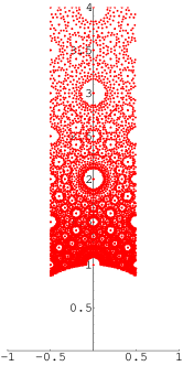
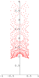
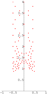
$L_{*}=150$		$L_{*}=50$		$L_{*}=20$

Figure 5: Vacuum distribution in the rigid Calabi–Yau model of [27, 28, 16] shown in the fundamental domain of the axi-dilaton moduli space. Depending on the value of $L_{*}$, D3-tadpole, the distribution of vacua in the moduli space can be either almost continuous or genuinely discrete.

For cases with small value of $L_{*}$, however, the continuous approximation is not very good, as in Figure 5 with $L_{*}=20$.

When the continuous approximation is not good, it is more appropriate to i) specify the set of points in ${\cal M}_{*}/\Gamma_{*}$ that admit integral fluxes, and ii) describe how many choices of such integral flux configurations are available at such points [16]. Suppose the dilaton vev $\left\langle{\phi}\right\rangle$ takes its value in an algebraic extension field ${\cal F}$ over $\mathbb{Q}$ with ${\cal D}:={\rm dim}_{\mathbb{Q}}{\cal F}=2$, and the complex structure moduli of $M_{3}$ are such that $[\Omega_{M_{3}}]\in{\cal F}\mathbb{P}[H^{3}(M_{3})]$ and $[D_{i}\Omega_{M_{3}}]\in{\cal F}\mathbb{P}[H^{3}(M_{3})]$ for $i=1,\cdots,h^{2,1}(M_{3})$. Then the number of flux quanta at our disposal (while preserving the F-term conditions) is

$$\kappa=4(h^{2,1}(M)_{-,{\rm prim.}}+1)-({\cal D}=2)\times(h^{2,1}(M)_{-,{\rm prim.}}+1),$$ (163)

which is reduced to

$$\kappa^{\prime}=4(h^{2,1}(M)_{-,{\rm prim.}}+1)-({\cal D}=2)\times(h^{2,1}(M)_{-,{\rm prim.}}+1)-({\cal D}=2)$$ (164)

when $\left\langle{W_{\rm GVW}}\right\rangle=0$ is required. Consequently, the number of flux configuration scales for a given complex structure $(\left\langle{\phi}\right\rangle,\left\langle{z^{a}}\right\rangle)$ as $(L_{*})^{\kappa/2}$ or $(L_{*})^{\kappa^{\prime}/2}$, respectively [16]. The overall number of flux vacua, estimated to be $(L_{*})^{2(h^{2,1}(M)_{-,{\rm prim.}}+1)}$, should be reproduced partially from $(L_{*})^{\kappa/2}$ times the number of such ${\cal D}=2$ vacua in the fundamental domain of the moduli space, and the rest must come from similar contributions from vacua with different value of the extension degree ${\cal D}$.

The $rk_{7}=16$ landscapes of F-theory on ${\rm K3}\times{\rm K3}$ in Section 5.2 fits very well with this discrete picture in two different ways. First, $L_{*}$ in the type IIB language comes from $\chi(Y_{4})/24$ in F-theory, which remains small for $Y_{4}={\rm K3}\times{\rm K3}$. This is visible most clearly in Figure 1, or in the relatively short list of vacuum points (there are 66) in the moduli space in Table 2 or merely 170 pairs found in the analysis of Section 5.2. These results definitely look closer to the $L_{*}=20$ picture in Figure 5 than the one with $L_{*}=150$.

The second reason is that the number of scanning flux quanta $\kappa$ available at each isolated point in ${\cal M}_{*}(J_{S},W_{\rm noscan})$ remains the same for all the $W_{\rm noscan}$-landscapes for F-theory on ${\rm K3}\times{\rm K3}$ with $rk_{7}={\rm rank}(W_{\rm noscan})=16$. This is obvious in the case of the $W_{\rm noscan}=(D_{4}^{\oplus 4});(\mathbb{Z}_{2}\times\mathbb{Z}_{2})$-landscape, because this is the type IIB orientifold compactification on $M_{3}=T^{2}\times K3$ with all the O7-planes accompanied by four D7-branes on top of them. But, even for other choices with ${\rm rank}(W_{\rm noscan})=16$, the number of scanning flux quanta $\kappa$, and hence the estimate of the number of ${\cal D}=2$ vacua should remain much the same, even if $W_{\rm noscan}$ contains $E_{6,7,8}$ type gauge group. The number of flux quanta freely scanned over for a given Kähler form (103) and a rank-16 $W_{\rm noscan}$ was

$$\kappa=8+2\times 17,\qquad\kappa^{\prime}=6+2\times 17$$ (165)

in the study in Section 5.2, which agrees with the type IIB orientifold value (163, 164) for $h^{2,1}(T^{2}\times{\rm K3})_{-,{\rm prim.}}=1+19$.

The action of the modular group $\Gamma_{*}$ is implemented in the continuous approximation of [27, 28] by simply restricting the complex $m$-dimensional restricted moduli space ${\cal M}_{*}$ to its fundamental region. If $L_{*}$ is small and one is in a situation of maintaining the discrete approach, one can still restrict the space ${\cal M}_{*}$ to its fundamental region under the action of the modular group $\Gamma_{*}$. Furthermore, one has to take a quotient of integral flux configurations admitted for a given point $[z]\in{\cal M}_{*}/\Gamma_{*}$ by the residual modular group $\Gamma_{*}(z)$, the stabilizer subgroup of a representative point $z\in{\cal M}_{*}$ [16]. In the example of type IIB on a rigid Calabi–Yau threefold [27, 28, 16], the first few axi-dilaton vevs for small flux contribution to the D3-tadpole sit at a special point in the axi-dilaton moduli space, $\left\langle{\phi}\right\rangle=i$, where the stabilizer subgroup of the moduli space $\Gamma_{*}={\rm SL}(2;\mathbb{Z})$ is non-trivial. Flux configurations for $\left\langle{\phi}\right\rangle=i$ have to be modded out by the non-trivial residual modular group.

Exactly the same phenomenon takes place in the case of compactification of F-theory on ${\rm K3}\times{\rm K3}$. For any point $(\omega_{X},\omega_{S})$ in the moduli space $D^{(X)}\times D^{(S)}$, the stabilizer subgroup of $\Gamma$ in (77) contains

$$\left(\left[W^{(2)}(S_{X})\rtimes{\rm Aut}(X)\right]\times\left[W^{(2)}(S_{S})\rtimes{\rm Aut}(S)\right]\right)\,.$$ (166)

${\cal M}_{*}(J_{S},W_{\rm noscan})$, however, further specifies an embedding of $[J_{S}]\in S_{S}\otimes\mathbb{R}/\mathbb{R}_{\geq 0}$ and $(U_{*}\oplus W_{\rm noscan})\subset S_{X}$. Thus, only the subgroup of (166) preserving this embedding remains as the residual modular group $\Gamma_{*}$ acting on the flux configuration. None of the reflection subgroup $W^{(2)}(S_{S})$ will be left in the residual modular group as long as $J_{S}$ is in the interior of the cone $\overline{{\rm Amp}}_{S}$. In our numerical study in Section 5.2 $J_{S}$ is sitting on a boundary of $\overline{{\rm Amp}}_{S}$, so that the $W_{E_{8}}\times W_{E_{8}}$ Weyl group in $W^{(2)}(S_{S})$ is in the residual modular group $\Gamma_{*}$. Similarly, most of $W^{(2)}(S_{X})$ is also gone from the residual modular group because of the embedding of $U_{*}\oplus W_{\rm noscan}$. At a point $\omega_{X}\in D^{(X)}$ where an extra non-Abelian factor of $W_{\rm root}$ emerges outside of $W_{\rm noscan}$, however, its Weyl group is still a part of $\Gamma_{*}$. The automorphisms in ${\rm Aut}(X)\cap\Gamma_{*}$ at least preserve the elliptic fibration morphism and the zero-section, so this is a small subgroup of ${\rm Aut}(X)$. We should also remark that our vacuum counting in Section 4.2 exploited all possible ${\rm Aut}(S)$ to take a quotient of the set of $G_{1}$-type fluxes. Since the argument there does not refer to the choice of $J_{S}$, one either has to count varieties in $J_{S}$ or use only the subgroup of ${\rm Aut}(S)$ preserving $J_{S}\in\overline{\rm Amp}_{S}$ when taking a quotient of the flux configurations.

In landscapes where $L_{*}$ is small, there is a pronounced void structure in the vacuum distribution on ${\cal M}_{*}/\Gamma_{*}$, and a significant fraction of vacua are accumulated at the special points at the centre of the voids [28, 16]. Sample statistics in Section 4.3 and, in particular, Section 5.2 must have been strongly influenced by this effect. Especially when it comes to the fraction of symmetric vacua in the statistics (such as the fraction of CP preserving vacua in Section 4.3), the small value of $L_{*}$ from $\chi(Y_{4})/24=24$ must have a strong impact. Keeping this in mind, one should not view the high fraction of CP symmetric vacua as a generic prediction of F-theory.

II From the perspective of F-theory, there is no reason to focus our attention only to $W_{\rm noscan}$-landscapes with $rk_{7}={\rm rank}(W_{\rm noscan})=16$. It is thus natural to discuss flux vacuum distribution on the restricted moduli space ${\cal M}_{*}(J_{S},W_{\rm noscan})$. In the rest of this section, we treat $\chi(Y_{4})/24$ (or $L_{*}$) as if it were a free parameter. By doing so, we can get a feeling for how the vacuum distribution depends on such parameters as $rk_{7}$—the rank of fixed 7-brane gauge groups—in F-theory compactification on general elliptic Calabi–Yau fourfolds (not necessarily ${\rm K3}\times{\rm K3}$). With this in mind, we use the continuous approximation to the space of flux quanta [27, 28, 16].

For ${\rm K3}\times{\rm K3}$, the restricted moduli space ${\cal M}_{*}(J_{S},W_{\rm noscan})$ is of complex dimension $m=(18-rk_{7})+19$. The vacuum index density (160) of [27, 28] in this set-up becomes an $(m,m)$-form on ${\cal M}_{*}$. Summation over the flux configuration is replaced by an integral, $d^{K}N$, and the delta functions (F-term condition) remove the integral over the $(3,1)+(1,3)$ Hodge components of the flux. Since we restrict the flux to be orthogonal to $W_{\rm noscan}$, there are only complex $m=(20-2-rk_{7})+(20-1)$ dimensions of such $(3,1)$ components to begin with, and hence all the integrals of the $(3,1)+(1,3)$ components are removed from $\int d^{K}N$ in (160). There are still remaining integrals over real $K-2m=2\times 2+(18-rk_{7})\times 19$ dimensions of the space of flux configuration; contribution to the D3-brane tadpole is positive definite in this space. This argument will lead to the vacuum index distribution that is an $(m,m)$-form $\rho_{\rm ind.}$ on ${\cal M}_{*}(J_{S},W_{\rm noscan})/\Gamma_{*}$ multiplied by a factor $(L_{*})^{K/2}$ with $K=[(20-rk_{7})\times 21]$. By requiring that $\left\langle{W_{\rm GVW}}\right\rangle=0$, $K$ is replaced by $K^{\prime}=K-2$. Therefore, the number of vacua in the ensemble of a given $W_{\rm noscan}$ and $J_{S}$ roughly scales as $(L_{*})^{-(21/2)\times rk_{7}}$ as a function of $rk_{7}$.

In order to study the ratio of the number of $\mathop{\rm SO}(10)$ vacua to $\mathop{\rm SU}(5)$ vacua in F-theory on ${\rm K3}\times{\rm K3}$ flux vacua, one should also address Kähler moduli stabilization, and the vacuum counting on the choice of $J_{S}$ need to be used as the weight multiplied on top of the distribution on ${\cal M}_{*}(J_{S},W_{\rm noscan})/\Gamma_{*}$. It will be arguable whether the ${\rm K3}\times{\rm K3}$ compactification of F-theory is phenomenologically interesting enough to motivate such a laborious study. Unless the weight factor from Kähler moduli stabilization contains very strong $rk_{7}$-dependence, it seems very difficult to overturn the statistical ratio of $(L_{*})^{-10.5}$ of $\mathop{\rm SO}(10)$ vacua to $\mathop{\rm SU}(5)$ vacua simply coming from the flux statistics for fixed $J_{S}$.

In such cases as $W_{\rm noscan}=A_{4}$ or $D_{5}$ in $Y=X\times S={\rm K3}\times{\rm K3}$ compactification of F-theory, there exists a primitive embedding $\phi:U\oplus W_{\rm noscan}\hookrightarrow\Lambda_{\rm K3}^{(X)}\cong H_{2}(X;\mathbb{Z})$. Furthermore, such an embedding is unique modulo ${\rm Isom}^{+}(\Lambda_{\rm K3}^{(X)})$ due to Theorem 1.14.4 of [98] and Theorem 2.8 of [77] (which is also quoted as Thm. $\epsilon$ in [25]). Thus, the restricted moduli space ${\cal M}_{*}$ can be constructed out of a single piece of the restricted period domain

$$\mathbb{P}\left[\left\{\left.\Omega_{X}\in(\Lambda_{\rm K3}^{(X)})^{*}\otimes\mathbb{C}\;\right|\;\Omega_{X}\wedge\Omega_{X}=0,\;\langle\Omega_{X},\phi(U\oplus W_{\rm noscan})\rangle=0,\;\Omega_{X}\wedge\overline{\Omega}_{X}>0\right\}\right].$$ (167)

If an attractive K3 surface $X=X_{[a~{}b~{}c]}$ admits an elliptic fibration whose $W_{\rm frame}$ contains a $W_{\rm noscan}$ as above, its $\Omega_{X}$ (equivalently a primitive embedding of its $T_{X}$ into $[\phi(U\oplus W_{\rm noscan})^{\perp}\subset\Lambda_{\rm K3}^{(X)}]$) should be found in this single piece of restricted period domain. Such an embedding of $T_{X}$, however, is no longer unique under the subgroup of ${\rm Isom}^{+}(\Lambda_{\rm K3})$ preserving the embedding $\phi:(U\oplus W_{\rm noscan})\hookrightarrow\Lambda_{\rm K3}^{(X)}$. In Sections 4.1 and 4.2.3, we discussed multiplicities of elliptic fibration on a given attractive K3 surface $X$ and a given isometry class of frame lattice. This multiplicity appears as a part of the non-uniqueness of the embedding of $T_{X}$ into $[\phi(U\oplus W_{\rm noscan})^{\perp}\subset\Lambda_{\rm K3}^{(X)}]$ modulo the remaining subgroup of ${\rm Isom}^{+}(\Lambda_{\rm K3})$.

III Having seen how the vacuum statistics depend on the rank of gauge groups, the next question of interest will be how it depends on the number of generations of matter fields. Since it is impossible to generate a non-zero net chirality on non-Abelian 7-branes in the ${\rm K3}\times{\rm K3}$ set-up, we content ourselves with studying the dependence on the number of vector-like pairs on a non-Abelian 7-brane. As we have seen in Section 5.3, the singular fibre fluxes generate some vector-like pairs of matter fields, while reducing the symmetry group on the non-Abelian 7-brane associated with the singular fibre. Thus, we set the problem as follows. For some choice of $J_{S}$ and $W_{\rm noscan}\subset W_{\rm frame}$ as before, let us specify

$$G_{\rm fix}=\sum_{A}(C_{A}\otimes F_{A}),\qquad C_{A}\in W_{\rm noscan}\cap W_{\rm root},\qquad F_{A}\in[J_{S}^{\perp}\subset S_{S}].$$ (168)

An ensemble of flux vacua is generated, by allowing the four-form flux $G^{(4)}$ to be $G_{\rm scan}+G_{\rm fix}$ for any $G_{\rm scan}$ orthogonal to $J_{S}$ and $W_{\rm noscan}$. The vacuum index density distribution of such a landscape is obtained as an $(m,m)$ form over the restricted moduli space ${\cal M}_{*}(J_{S},W_{\rm noscan})/\Gamma_{*}$. Landscapes with different $G_{\rm fix}$ share the same restricted moduli space as long as $W_{\rm noscan}$ and $J_{S}$ remain the same. When we take $W_{\rm noscan}$ to be $E_{7}$, $E_{6}$ or $D_{5}$, for example, and $G_{\rm fix}=(C_{A}\otimes F_{A})$ so that the unbroken symmetry becomes $E_{6}$, $D_{5}$ or $A_{4}$, the singular fibre flux $G_{\rm fix}$ determines the number of vector-like pairs in the ${\bf 27}+\overline{\bf 27}$, ${\bf 16}+\overline{\bf 16}$ and ${\bf 10}+\overline{\bf 10}$ representations, respectively, through (154). By comparing the numbers of vacua of the ensembles of $(J_{S},W_{\rm noscan};G_{\rm fix})$ with the common $(J_{S},W_{\rm noscan})$ and different $G_{\rm fix}$, we can determine the statistical cost of leaving vector-like pairs of matter fields in certain classes of representations in the effective theory.

The result is simple. Our estimate of the number of vacua in such an ensemble is given by

$$(L_{*,{\rm eff}.})^{K^{\prime}/2};\qquad L_{*,{\rm eff.}}=\frac{\chi(X\times S)}{24}-\frac{1}{2}(G_{\rm fix})^{2},$$ (169)

replacing $L_{*}=\chi(Y)/24$ by the remaining D3-tadpole $L_{*,{\rm eff.}}$ to be cancelled by the flux other than $G_{\rm fix}$. The more the number of vector-like pairs, the less the effective value $L_{*,{\rm eff}.}$. If $L_{*}=\chi(Y)/24$ were fairly large (and $K^{\prime}/2$ is not particularly large), then requiring one or two vector-like pairs of the matter field does not reduce the number of vacua too much, relatively. If $L_{*}$ is not particularly large, then the number of vacua with a few more vector-like pairs of matter fields becomes much smaller. Clearly, this effect is further enhanced when $K^{\prime}/2$ is large.

IV Finally, let us study the $(m,m)$-form distribution $\rho_{\rm ind.}$ over ${\cal M}_{*}/\Gamma_{*}$ in the context of F-theory compactification, not just the overall number of flux vacua. We begin with a review of what is known about $\rho_{\rm ind}$ in [27, 28, 2].

The most robust result on $\rho_{\rm ind}$ states that, for F-theory compactification without much restriction on the space of scanning four-form fluxes $G^{(4)}_{\rm scan}$, $\rho_{\rm ind}$ is written in the form of the Euler class $e(\nabla)$ on ${\cal M}_{*}$ (which means that it is a differential $2m$-form) associated with a connection $\nabla$ on a real vector bundle with rank $2m$ [2]. The formula [27, 28]

$$\rho_{\rm ind}={\rm det}\left(-\frac{R}{2\pi i}+\frac{\omega}{2\pi}{\bf 1}\right)_{m\times m}=e(T{\cal M}_{*}\otimes{\cal L}^{-1})=c_{n}(T{\cal M}_{*}\otimes{\cal L}^{-1}),$$ (170)

is a special case of the more robust result $\rho_{\rm ind}=e(\nabla)$ [2]. Here, $\omega$ is the Kähler form and $R$ the curvature $(1,1)$ form of the holomorphic vector bundle $T{\cal M}_{*}$, ${\cal L}$ is the line bundle whose first Chern class is $-\omega/(2\pi)$ and $c={\rm det}(-kR/(2\pi i)+{\bf 1})=\sum_{k}c_{k}t^{k}$ defines the Chern classes. It takes an extra effort to find for which real vector bundle $\rho_{\rm ind}=e(\nabla)$ for general cases.

It is known that the formula (170) can be used at least for two categories of landscapes.

• : type IIB on a Calabi–Yau orientifold $M_{3}$ with full scanning of three-form fluxes $G^{(3)}_{\rm scan}$ and with all the D7-branes appearing as an $\mathop{\rm SO}(8)$ configuration [28], i.e. four D7-branes on each O7-plane.

• : F-theory compactification on a Calabi–Yau fourfold $Y_{4}$ with the four-form flux scanning in a sufficiently large space.

An example of category B is given by [2]:

$$G^{(4)}_{\rm scan}\in\left[H^{4,0}(Y;\mathbb{C})+{\rm h.c.}\right]\oplus\left[H^{3,1}(Y;\mathbb{C})_{\rm prim.}+{\rm h.c.}\right]\oplus\left[\left(H^{2,2}(Y;\mathbb{R})_{V}\right)^{\perp}\subset H^{2,2}(Y;\mathbb{R})\right]\,.$$ (171)

Here, $H^{(2,2)}(Y;\mathbb{R})_{V}$ is the subspace of $H^{2,2}(Y;\mathbb{R})$ spanned by the intersection of any pair of divisors of $Y$ (this naive definition is made more precise shortly).

Let us explain what we mean by a “sufficiently large space” when we introduced category B. Let $V\subset H^{4}(Y;\mathbb{R})$ be the subspace in which the four-form is scanned to generate a landscape, and let $\{\psi_{I=1,2,\cdots}\}$ be a basis of $V$. The assumption made (implicitly) in [2] is that the vector space $V$ is large enough that one can make a replacement

$$\left(\int_{Y}\psi_{I}\wedge\varphi\right)(A^{-1})^{IJ}\left(\int_{Y}\psi_{J}\wedge\chi\right)\Longrightarrow\int_{Y}\varphi\wedge\chi,\qquad A_{IJ}:=\int_{Y}\psi_{I}\wedge\psi_{J}$$ (172)

for arbitrary differential forms $\psi$ and $\chi$ that belong to the vector space

$$G^{(4)}_{\rm scan}\in\left[H^{4,0}(Y_{z};\mathbb{C})+H^{0,4}(Y_{z};\mathbb{C})\right]\oplus\left[H^{3,1}(Y_{z};\mathbb{C})_{*}+H^{1,3}(Y_{z};\mathbb{C})_{*}\right]\oplus H^{2,2}(Y_{z};\mathbb{R})_{H*}\,.$$ (173)

The quantities $[H^{3,1}(Y_{z};\mathbb{C})_{*}$ and $H^{2,2}(Y_{z};\mathbb{R})_{H*}$ are defined in the next paragraph and (175).

It is a natural generalization of the category B landscapes above to require extra divisors corresponding to extra 7-brane gauge groups, i.e. introduce a $W_{\rm noscan}$ as done earlier in this section. The moduli space ${\cal M}_{*}(J_{Y},W_{\rm noscan})$ is then reduced in dimensions from the full space of complex structure moduli of $Y$ compatible with a Kähler form $J_{Y}$. The $H^{3,1}+H^{1,3}$ components of the flux is then not only required to be primitive, $G^{(4)}_{\rm scan}\wedge J_{Y}=0$, but the same condition is required with regard to the divisors in $W_{\rm noscan}$. Let $[H^{3,1}(Y_{z};\mathbb{C})_{*}+H^{1,3}(Y_{z};\mathbb{C})_{*}]$ denote the resulting smaller subspace. The $(H^{2,2}_{V})^{\perp}$ component of the flux space is also reduced, because $H^{2,2}(Y_{z};\mathbb{R})_{V}$ is larger in dimensions. This new $H^{2,2}(Y_{z};\mathbb{R})_{V}$ is denoted by $H^{2,2}(Y_{z};\mathbb{R})_{V*}$. We then have an ensemble of vacua with the four-form flux scanning over the vector space

$$G^{(4)}_{\rm scan}\in\left[H^{4,0}(Y;\mathbb{C})+{\rm h.c.}\right]\oplus\left[H^{3,1}(Y;\mathbb{C})_{*}+{\rm h.c.}\right]\oplus\left[\left(H^{2,2}(Y;\mathbb{R})_{V*}\right)^{\perp}\subset H^{2,2}(Y;\mathbb{R})\right];$$ (174)

Let us refer to these landscapes as category B’.

In order to state the relation between the category A landscapes and category B’ landscapes, we need to prepare the following language. Consider a family of Calabi–Yau fourfolds $\pi:{\cal Y}\longrightarrow{\cal M}_{*}$, where $Y_{z}:=\pi^{-1}(z)$ is the Calabi–Yau fourfold corresponding to $z\in{\cal M}_{*}$. We have in mind a restricted moduli space ${\cal M}_{*}$ for a specific choice of Kähler form $J_{Y}$ and some set of divisors $W_{\rm noscan}$ corresponding to the 7-brane gauge groups. The $H^{2,2}(Y_{z};\mathbb{R})$ vector space over $\mathbb{R}$ for each $z\in{\cal M}_{*}$ is decomposed as follows. First, $H^{2,2}(Y_{z};\mathbb{R})_{V*}$ is defined as the subspace spanned by intersection of $Y_{z}$ with any pair of divisors of ${\cal Y}$. Secondly, another subspace $H^{2,2}(Y_{z};\mathbb{R})_{H*}\subset H^{2,2}(Y_{z};\mathbb{R})$ is defined as

$${\rm Span}_{\mathbb{C}}\left\{(D_{a}D_{b}\Omega_{Y}),\overline{(D_{c}D_{d}\Omega_{Y})}\right\}|_{a,b,c,d\in 1,\cdots,m}\cap H^{2,2}(Y_{z};\mathbb{R})\,,\hskip 14.22636ptm={\rm dim}\,{\cal M}_{*}\,.$$ (175)

It is known that [2]

• the vector space of (2,2) Hodge components is divided into $H^{2,2}_{\ell=0}\oplus H^{2,2}_{\ell=1}\oplus H^{2,2}_{\ell=2}$

• the intersection form is positive definite on $H^{2,2}_{\ell=0}\oplus H^{2,2}_{\ell=2}$ and negative definite on $H^{2,2}_{\ell=1}$

• $H^{2,2}_{\ell=1}\oplus H^{2,2}_{\ell=2}$ is contained in $H^{2,2}(Y_{z};\mathbb{R})_{V*}$

The differential forms in the first component, $H^{2,2}_{\ell=0}$ are the primitive $(2,2)$ forms. Thus, the intersection form is positive definite on the orthogonal complement $[(H^{2,2}(Y_{z};\mathbb{R})_{V*})^{\perp}\subset H^{2,2}(Y_{z};\mathbb{R})]$, and there is a well-defined orthogonal decomposition of the $H^{2,2}(Y_{z};\mathbb{R})$ vector space:

$$H^{2,2}(Y_{z};\mathbb{R})=H^{2,2}(Y_{z};\mathbb{R})_{H*}\oplus H^{2,2}(Y_{z};\mathbb{R})_{RM}\oplus H^{2,2}(Y_{z};\mathbb{R})_{V*}.$$ (176)

Note that the remnant subspace $H^{2,2}(Y_{z};\mathbb{R})_{RM}$ is not empty in general [99]. In particular, as explained in detail in Appendix C, this happens already in the case of $Y={\rm K3}\times{\rm K3}$. As discussed in Appendix C, the landscape of category A (roughly speaking, type IIB orientifolds with three-form scanning (241)) corresponds to scanning the four-form in the $H^{2,2}(Y;\mathbb{R})_{H*}$ subspace in addition to the first two components of (171), i.e., the space (235). This is a smaller subspace than (174), in principle, in the sense that $H^{2,2}(Y;\mathbb{R})_{RM}$ can be non-empty. This indicates that the scanning space of the flux can be sufficiently large, for the condition (172) to hold (and the formula (170) also holds consequently), even when the scanning space is smaller than (174).

As discussed in Appendix C, the four-form scanning we have introduced in this section also corresponds to the vector space (235). It is thus reasonable to think of one more category of landscapes in F-theory which contains both the category A landscapes and the ones on $Y={\rm K3}\times{\rm K3}$ with arbitrary $rk_{7}$ we have considered. Let us call category A’ any landscapes generated by scanning four-form flux in the vector space (235) for an elliptic fibred Calabi–Yau fourfold $\pi_{Y}:Y\rightarrow B_{3}$. This is to be contrasted with those in category B’ where the four-form flux is scanned in (174).

It must now be obvious that the formula (170) holds, not just for the landscapes in category B’, but also for the landscapes in category A’. Since the condition (172) requires that $\psi_{I}(A^{-1})^{IJ}\psi_{J}$ be an insertion of a complete system only for $\varphi,\chi$ in (235), it is equivalent to say that the entire vector space (235) is contained in the space of four-form scanning (or not). Appendix C also provides an alternative (more down to earth) derivation of the formula (170) following the line of argument in one of the original articles [28]), rather than the refined version of [2], with an assumption (245) and a little more concrete consequence (261). We understand that the argument here is enough to justify the formula (170) for landscapes in category A’.

There is an immediate consequence of this observation. Any landscape (an ensemble of vacua) in category B’ is decomposed into multiple landscapes (ensembles of vacua) in category A’ labelled by $G^{(4)}_{\rm fix}$ in $H^{2,2}(Y;\mathbb{R})_{\rm RM}$. Since all of these landscapes in category A’ share the same restricted moduli space ${\cal M}_{*}$, and since the formula (170) determines $\rho_{\rm ind}$ only in terms of geometry of ${\cal M}_{*}$, the vacuum index distribution $d\mu_{I}$ for these landscapes in category A’ are the same apart form the $G^{(4)}_{\rm fix}$-dependent overall normalization (169).

Let us use (170) to derive an explicit result on the distribution of moduli parameters. Consider a landscape of F-theory compactification on $Y=X\times S={\rm K3}\times{\rm K3}$ with some rank-16 $W_{\rm noscan}$ and $G^{(4)}_{\rm fix}$. Then the restricted moduli space is of the form ${\cal M}_{*}={\cal M}_{\rho_{1}}\times{\cal M}_{\rho_{2}}\times{\cal M}_{\rm K3}(S;J_{S})$. This is because the lattice $[(U_{*}\oplus W_{\rm noscan})^{\perp}\subset H^{2}(X;\mathbb{Z})]$ is always signature $(2,2)$, and the intersection form can be made $U\oplus U$ for some $\mathbb{R}$-coefficient basis of the vector space obtained by tensoring $\mathbb{R}$ with the signature $(2,2)$ lattice above. The Kähler forms of the moduli spaces ${\cal M}_{\rho_{1}}$ and ${\cal M}_{\rho_{2}}$ are $K^{(\rho_{1})}=-\ln[(\rho_{1}-\bar{\rho}_{1})/i]$ and $K^{(\rho_{2})}=-\ln[(\rho_{2}-\bar{\rho}_{2})/i]$, respectively. The modulus $\rho_{1}$ is interpreted as the axi-dilaton of type IIB orientifold in the case of $W_{\rm noscan}=D_{4}^{\oplus 4};(\mathbb{Z}_{2}\times\mathbb{Z}_{2})$. By closely following the computation of Section 3.1.2 in [28], we obtain

$$\rho_{\rm ind} = \left(-\frac{R^{(\rho_{1})}}{2\pi i}+\frac{\omega^{(S)}}{2\pi}+\frac{\omega^{(\rho_{1})}}{2\pi}+\frac{\omega^{(\rho_{2})}}{2\pi}\right)\wedge\left(-\frac{R^{(\rho_{2})}}{2\pi i}+\frac{\omega^{(S)}}{2\pi}+\frac{\omega^{(\rho_{1})}}{2\pi}+\frac{\omega^{(\rho_{2})}}{2\pi}\right)\wedge$$ (177)

$$\qquad{\rm det}\left(-\frac{R^{(S)}}{2\pi i}+\left(\frac{\omega^{(S)}}{2\pi}+\frac{\omega^{(\rho_{1})}}{2\pi}+\frac{\omega^{(\rho_{2})}}{2\pi}\right){\bf 1}\right),$$

$$= 2\frac{\omega^{(\rho_{1})}}{2\pi}\wedge\frac{\omega^{(\rho_{2})}}{2\pi}\wedge\left\{c_{m-2}^{(S)}+\left(\frac{\omega^{(S)}}{2\pi}\right)^{2}\wedge c_{m-4}^{(S)}\right\},$$ (178)

where $\omega^{(\rho_{1})}$, $\omega^{(\rho_{2})}$ and $\omega^{(S)}$ are the Kähler forms on the moduli spaces ${\cal M}_{\rho_{1}}$, ${\cal M}_{\rho_{2}}$ and ${\cal M}_{\rm K3}(S;J_{S})$, respectively, and $R^{(S)}$, $R^{(\rho_{2})}$ and $R^{(\rho_{1})}$ the curvature $(1,1)$-forms of the tangent bundles of those moduli spaces . $c_{r}^{(S)}$’s are the $r$-th Chern class of the holomorphic rank-$(m-2)$ vector bundle $T{\cal M}_{\rm K3}(S;J_{S})\otimes({\cal L}^{(S)})^{-1}$, where ${\cal L}^{(S)}$ is the line bundle whose first Chern class is $-\omega^{(S)}/2\pi$. Thus, in these set-ups the vacuum index density distribution $\rho_{\rm ind.}$ is factorized for the three pieces of the moduli space. If one is interested only in the distribution of any one among $\rho_{1}$, $\rho_{2}$ and moduli of the K3 surface $S$, but not altogether, then the distribution $\rho_{\rm ind}$ can be integrated over the irrelevant coordinates first. For the moduli $\rho_{1}$ and $\rho_{2}$, in particular,

$$\rho_{\rm ind.}(\rho_{1})\propto d[{\rm Re}\rho_{1}]d[{\rm Im}\rho_{1}]\frac{1}{({\rm Im}(\rho_{1}))^{2}},\qquad\qquad\rho_{\rm ind.}(\rho_{2})\propto d[{\rm Re}\rho_{2}]d[{\rm Im}\rho_{2}]\frac{1}{({\rm Im}(\rho_{2}))^{2}}.$$ (179)

Applying this result to the $W_{\rm noscan}=E_{8}\oplus E_{8}$-landscape, in particular, the prediction in the continuous approximation (179) for $\rho_{2}$ can also be read as that of $[{\rm vol}(T^{2})/\ell_{s}^{2}]_{\rm Het}$. Our numerical results (not relying on continuous approximation) in Section 5.2 agree with this prediction based on the continuous approximation qualitatively in that large ${\rm Im}(\tilde{\rho}_{H})=[{\rm vol}(T^{2})/\ell_{s}^{2}]_{\rm Het}$ is statistically disfavoured. Note that this happens although we should not expect the continuous approximation to be very good because $\chi(Y)/24=24$ is not particularly large.

The result (179) also indicates that there is no correlation between the distribution of $\rho_{1}$, $\rho_{2}$ and the moduli of K3 surface $S$, if we ignore the difference between the vacuum distribution and the vacuum index distribution. Figure 4 (iii) in Section 5.2 may be regarded as a manifestation of the absence of any correlation between $\rho_{1}$ and $\rho_{2}$.

It is an interesting question how $\rho_{\rm ind}$ depends on ${\rm Im}(\tilde{\rho}_{H})$ for different values of $rk_{7}$. $\rho_{\rm ind}$ is not expected to have a factorized form as (179), but it will be in the form of

$$\rho_{\rm ind}=c_{18-rk_{7}}^{(X)}c_{19}^{(S)}+\omega^{(X)}\omega^{(S)}c_{17-rk_{7}}^{(X)}c_{18}^{(S)}+(\omega^{(X)}\omega^{(S)})^{2}c_{16-rk_{7}}^{(X)}c_{17}^{(S)}+\cdots,$$ (180)

where $c_{r}^{(X)}$’s are the $r$-th Chern class of the rank-$(18-rk_{7})$ holomorphic vector bundle $T{\cal M}_{\rm K3}(X;U_{*}\oplus W_{\rm noscan})\otimes{\cal L}_{(X)}^{-1}$. It must still be possible to extract the leading power-law behaviour in ${\rm Im}(\tilde{\rho}_{H})$ in the large ${\rm Im}(\tilde{\rho}_{H})$ region of the moduli space, using the parametrization (186). We leave this as an open problem in this article.

Acknowledgements

We thank Kazuo Hosomichi for useful comments, and Tetsuji Shioda for giving a lecture on Mordell–Weil lattice on K3 surface, in January 2010 at IPMU, Tokyo. A. P. B. likes to thank the IPMU Tokyo for kind hospitality during his visit in summer of 2012, which initiated this collaboration. The work of A. P. B. was supported by a JSPS postdoctoral fellowship under grant PE 12530, and by the STFC under grant ST/J002798/1 and that of T. W. by WPI Initiative, MEXT, Japan and a Grant-in-Aid for Scientific Research on Innovative Areas 2303.

Appendix A A Note on Heterotic String Narain Moduli

Although Narain compactificaiton of heterotic string theory is a well-known subject, we leave a brief note here for summary of conventions used in the main text of this article.

A compactification of heterotic string theory on $T^{2}$ is specified by embedding an even self-dual lattice ${\rm II}_{2,18}$ in a space

$$\mathbb{R}^{2,18}=\left\{\sqrt{\frac{\alpha^{\prime}}{2}}(k^{R}_{8},k^{R}_{9},k^{L}_{8},k^{L}_{9},k_{i=11,\cdots,26})^{T}\right\}$$ (181)

where the metric on $\mathbb{R}^{2,18}$ is $\mathop{\rm diag}\nolimits({\bf 1}_{2\times 2},{\bf 1}_{18\times 18})$. Let $\{e_{K8},e_{\bar{w}8},e_{K9},e_{\bar{w}9},e_{I=11,\cdots,26}\}$ be a set of generators of ${\rm II}_{2,18}$ (as well as its image in $\mathbb{R}^{2,18}$) where $U={\rm Span}_{Z}\{e_{K8},e_{\bar{w}8}\}$, $U={\rm Span}_{\mathbb{Z}}\{e_{K9},e_{\bar{w}9}\}$, and $E_{8}\oplus E_{8}$ is generated by the rest, $\{e_{I=11,\cdots,26}\}$. Thus, the data of this compactification is written in the form of a $(2+18)\times(2+2+16)$ matrix,

$${\cal Z}=\left[e_{K8},e_{\bar{w}8},e_{K9},e_{\bar{w}9},e_{I=11},\cdots,e_{I=26}\right],\qquad{\cal Z}^{T}\cdot\left(\begin{array}[]{cc}{\bf 1}_{2\times 2}&\\ &-{\bf 1}_{18\times 18}\end{array}\right)\cdot{\cal Z}=\left(\begin{array}[]{cccc}U&&&\\ &U&&\\ &&C_{E_{8}}&\\ &&&C_{E_{8}}\end{array}\right),$$ (182)

where the $U$ in (182) denotes the matrix $\left[\begin{array}[]{cc}&1\\ 1&\end{array}\right]$ and $C_{E_{8}}$ the negative of the Cartan matrix of $E_{8}$, which is also the (negative definite) intersection form of the $E_{8}$ root lattice. General elements of ${\rm II}_{2,18}$ are written in the form of $n_{8}e_{K8}+(-w^{8})e_{\bar{w}8}+n_{9}e_{K9}+(-w^{9})e_{\bar{w}9}+\sum_{I}q^{I}e_{I}$, which is also denoted by $(n_{8},-w^{8},n_{9},(-w^{9}),q^{I})^{T}$ in the component description. The generators $e_{K8,K9}$ correspond to states with elementary Kaluza–Klein excitation in $T^{2}$, and $e_{\bar{w}8,\bar{w}9}$ to states winding $T^{2}$ once.

The first two rows of the matrix ${\cal Z}$ are denoted by ${\cal Z}^{R}_{m}$ with $m=8,9$. Introducing ${\cal Z}^{R}:={\cal Z}^{R}_{8}+i{\cal Z}^{R}_{9}$, it follows from relation (182) that

$${\cal Z}^{R}\cdot\left(\begin{array}[]{cccc}U^{-1}&&&\\ &U^{-1}&&\\ &&(C_{E_{8}})^{-1}&\\ &&&(C_{E_{8}})^{-1}\end{array}\right)\cdot\left({\cal Z}^{R}\right)^{T}=0\,.$$ (183)

Because ${\cal Z}^{R}$ can be regarded as an element of ${\rm Hom}({\rm II}_{2,18},\mathbb{C})$,

$${\cal Z}^{R}:(n_{8},-w^{8},n_{9},-w^{9},q^{I})^{T}\longmapsto\sqrt{\frac{\alpha^{\prime}}{2}}(k^{R}_{8}+ik^{R}_{9})\;{\rm component~{}of}\;(e_{K8}n^{8}+e_{\bar{w}8}(-w^{8})+\cdots+\sum_{I}e_{I}q^{I}),$$

we see that the relation above can also be written as $({\cal Z}^{R},{\cal Z}^{R})=0$ using the symmetric pairing of the dual lattice ${\rm II}_{2,18}^{*}$ naturally extended bilinearly to ${\rm II}_{2,18}^{*}\otimes\mathbb{C}$. With the same notation, it also follows that

$$({\cal Z}^{R},\overline{{\cal Z}^{R}})=+2.$$ (184)

The moduli space of this Narain compactification is parametrized by 18 complex numbers. With a parametrization that is understood intuitively in the supergravity approximation of heterotic $E_{8}\times E_{8}$ string theory, $k^{R}_{m=8,9}$ in ${\cal Z}^{R}$ are written as follows [100]:

$$k^{R}_{m}=\frac{n_{m}}{R_{m}}-\frac{R_{m}w^{m}}{\alpha^{\prime}}-\sum_{I}q^{I}A_{I,m}+\frac{1}{2}\sum_{I,J}A_{I,m}C^{IJ}(\sum_{n}w^{n}R_{n}A_{J,n});\qquad({\rm no~{}summation~{}in~{}}m)$$ (185)

$A_{I,m}$’s ($m=8,9$ and $I=11,\cdots,26$) are the Wilson lines on $T^{2}$ for the simple roots of $E_{8}\times E_{8}$, and $R_{m=8,9}$ the radii of the two directions of $T^{2}$. Together with two more $\mathbb{R}$-valued parameters that we have omitted here ($\left\langle{B}\right\rangle=0$, and $T^{2}$ is rectangular, just for better readability), there are $2\times 18$ parameters in total. $C^{IJ}$ is the inverse of the matrix $C_{E_{8}\times E_{8}}$. Therefore, ${\cal Z}^{R}$ is parametrized by 18 complex numbers. In the component description of $[U\oplus U\oplus E_{8}\oplus E_{8}]^{*}\otimes\mathbb{C}$, it is given by

$${\cal Z}^{R}=\frac{i}{\sqrt{2{\rm Im}(\tau_{H}){\rm Im}(\tilde{\rho}_{H})+{\rm Im}(a_{P})C^{PQ}{\rm Im}(a_{Q})}}(-\tau_{H},\;-\tilde{\rho}_{H},\;1,\;-\tau_{H}\tilde{\rho}_{H}-a_{K}C^{KL}a_{L}/2,\;a_{I}),$$ (186)

where (under the condition that $\left\langle{B}\right\rangle=0$ and $T^{2}$ is rectangular)

$$\tau_{H}=i\frac{R_{9}}{R_{8}},\quad\rho_{H}=i\frac{R_{8}R_{9}}{\alpha^{\prime}},\quad a_{I}=iR_{9}(A_{I,8}+iA_{I,9})=\sqrt{\alpha^{\prime}\tau_{H}\rho_{H}}(A_{I,8}+iA_{I,9}),$$ (187)

and

$$\qquad\tilde{\rho}_{H}=\rho_{H}-\frac{a_{I}C^{IJ}(a-\bar{a})_{J}}{4i\,{\rm Im}(\tau_{H})}.$$ (188)

Appendix B Heterotic Cartan Flux and Semistable Degeneration

B.1 Set-up

In this appendix, the discussion on heterotic–F-theory duality of Cartan/Mordell–Weil flux of Section 5.3 is made explicit by using the two-parameter family of K3 surfaces (99, 100) for F-theory (and its heterotic dual) as an example.

If we are to require a pair of ${\rm IV}^{*}$ singular fibres, this specifies a family of $\rho_{X}=12+2=14$ K3 surfaces, whose moduli space has dimension 6. Let

$$T_{X}^{\rho=14}=U\oplus U\oplus A_{2}\oplus A_{2},\qquad W_{\rm frame}^{\rho=14}=E_{6}\oplus E_{6}.$$ (189)

The two parameter family of K3 surfaces, $X={\rm Km}(E_{\rho_{1}}\times E_{\rho_{2}})$, has four more independent algebraic cycles, $\rho_{X}=18$, and the transcendental lattice is only of rank 4, $T_{X}^{\rho=18}=U[2]\oplus U[2]$. Such a special family of K3 surfaces can be identified by an embedding $T_{X}^{\rho=18}\longrightarrow T_{X}^{\rho=14}$:

$$(\overline{C}_{32},\overline{C}_{14},\overline{C}_{12},\overline{C}_{43})\longmapsto(v,V,v^{\prime},V^{\prime},\alpha^{\rm v}_{1},\alpha^{\rm v}_{2},\alpha^{\rm h}_{1},\alpha^{\rm h}_{2})\left[\begin{array}[]{cc|cc}1&1&&\\ &2&&\\ \hline\cr&&1&1\\ &&&2\\ \hline\cr&1&&\\ &&&1\\ \hline\cr&-1&&\\ &&&1\end{array}\right],$$ (190)

where $\overline{C}_{32,14,12,43}$ are generators of $T_{X}^{\rho=18}=U[2]\oplus U[2]$, $\{v,V,v^{\prime},V^{\prime}\}$ those of $U\oplus U\subset T_{X}^{\rho=14}$, and $\{\alpha^{\rm v}_{1,2}\}$ and $\{\alpha^{\rm h}_{1,2}\}$ those of the structure group $A_{2}=\mathop{\rm SU}(3)$ in the visible and hidden sectors, respectively.

In this two parameter family of K3 surfaces (Kummer surfaces), the four extra independent algebraic cycles are the generators of the orthogonal complement of the image of $T_{X}^{\rho=18}$ within $T_{X}^{\rho=14}$. This lattice is also regarded as the orthogonal complement of the $E_{6}\oplus E_{6}$ lattice within the frame lattice $W^{\rho=18}$ for $\rho=18$. Hence this is also the essential lattice $L(X)=W_{{\rm U}(1)}$ of this elliptic fibration. $L(X)=W_{{\rm U}(1)}$ is generated by

$$(P,Q,P^{\prime},Q^{\prime})=(v,V,v^{\prime},V^{\prime},\alpha^{\rm v}_{1},\alpha^{\rm v}_{2},\alpha^{\rm h}_{1},\alpha^{\rm h}_{2})\left[\begin{array}[]{cc|cc}&2&&-1\\ &&&\\ \hline\cr-1&&2&\\ &&&\\ \hline\cr 1&1&&\\ &&1&1\\ \hline\cr 1&-1&&\\ &&1&-1\end{array}\right].$$ (191)

The period integral is therefore in the form of

$${\cal Z}^{R}\propto\Omega_{X}=\left(-\tau_{H},-\tilde{\rho}_{H};1,-\tau_{H}\tilde{\rho}_{H}+\frac{\tau^{2}_{H}+1}{2};\tau_{H}+\frac{1}{2},-\left(\frac{\tau_{H}}{2}+1\right),0^{6};-\left(\tau_{H}-\frac{1}{2}\right),\frac{\tau_{H}}{2}-1,0^{6}\right)$$ (192)

in the component description of $[U\oplus U\oplus E_{8}\oplus E_{8}]^{*}\otimes\mathbb{C}$. In the component description using $(T_{X}^{\rho=18})^{*}\otimes\mathbb{C}$ (and irrelevant $(W_{{\rm U}(1)}\oplus E_{6}\oplus E_{6})^{*}\otimes\mathbb{C}$), this becomes

$$\left(-\tau_{H},-(2\tilde{\rho}_{H}-\tau_{H}),1,-\tau_{H}(2\tilde{\rho}_{H}-\tau_{H})\right).$$ (193)

Thus, in the parametrization of $\Omega_{X}$ in terms of $\tau_{H}$ and $\tilde{\rho}_{H}$, the K3 surface $X={\rm Km}(E_{\rho_{1}}\times E_{\rho_{2}})$ varies as

$$\rho_{1}=\tau_{H},\qquad\rho_{2}=2\tilde{\rho}_{H}-\tau_{H}.$$ (194)

Obviously the parametrization (192) follows the convention of Narain moduli for heterotic string compactification, and the correspondence (194) should be read as the duality map between the coordinates of the heterotic and F-theory moduli spaces.

In the heterotic string language, the component description of ${\cal Z}^{R}$ in (192) is a manifest consequence of the condition (147), with the flux data $n_{A}$’s in (146) given by the $k=4$ column vectors in (191). The Wilson lines are constrained to be torsion points in ${\rm Jac}(T^{2})$ of the heterotic compactification:

$$\mathop{\rm diag}\nolimits\left(\frac{\tau_{H}}{2},-\frac{\tau_{H}+1}{2},\frac{1}{2}\right)\subset\mathfrak{su}(3)^{\rm vis.},\qquad\mathop{\rm diag}\nolimits\left(-\frac{\tau_{H}}{2},\frac{\tau_{H}-1}{2},\frac{1}{2}\right)\subset\mathfrak{su}(3)^{\rm hid.}.$$ (195)

Wilson lines in the dimension-3 representations of the structure group $\mathop{\rm SU}(3)^{\rm vis.}\times\mathop{\rm SU}(3)^{\rm hid.}$ take values in 2-torsion points in this case, which is also the direct consequence of the spectral surface equations $a^{\rm v}_{3}y=0$ for the visible sector and $a^{\rm h}_{3}y=0$ for the hidden sector.

B.2 Mordell–Weil Group and Narrow Mordell–Weil Group

In the two parameter family of K3 surfaces $X={\rm Km}(E_{\rho_{1}}\times E_{\rho_{2}})$ with an elliptic fibration of type $2{\rm IV}^{*}+8I_{1}$, the essential lattice is

$$L(X)=W_{{\rm U}(1)}\cong A_{2}[2]\oplus A_{2}[2]\cong{\rm Span}_{\mathbb{Z}}\{P,P^{\prime}\}\oplus{\rm Span}_{\mathbb{Z}}\{Q,Q^{\prime}\}.$$ (196)

$E_{6}\oplus E_{6}$ forms the root lattice $W_{\rm root}$ of the frame lattice $W_{\rm frame}$ for generic $\rho_{1}$ and $\rho_{2}$, and the frame lattice is obtained by adding, to $W_{\rm root}\oplus W_{{\rm U}(1)}$, such glue vectors as

$$\frac{2P+P^{\prime}}{3}+\omega^{\rm v}_{\bf 27}+\omega^{\rm h}_{\bf 27},\qquad\frac{P+2P^{\prime}}{3}+\omega^{\rm v}_{\overline{\bf 27}}+\omega^{\rm h}_{\overline{\bf 27}}$$ (197)

$$\frac{2Q+Q^{\prime}}{3}+\omega^{\rm v}_{\bf 27}+\omega^{\rm h}_{\overline{\bf 27}},\qquad\frac{Q+2Q^{\prime}}{3}+\omega^{\rm v}_{\overline{\bf 27}}+\omega^{\rm h}_{{\bf 27}},$$ (198)

where $\omega_{\bf 27}^{\rm v,h}$ [resp. $\omega_{\overline{\bf 27}}^{\rm,h}$] are the weights of the ${\bf 27}$ [resp. $\overline{\bf 27}$] representation of the visible/hidden sector $E_{6}$ symmetry. The quotient space $W_{\rm frame}/W_{\rm root}\cong MW(X)\cong\mathbb{Z}^{\oplus 4}$ is generated by those four elements and the height pairing of the Mordell–Weil lattice is $A_{2}^{*}[-2]\oplus A_{2}^{*}[-2]$ in this basis (as is well-known in the literature).

Reference [85] provides explicitly expressions of four generators of $MW(X)\cong\mathbb{Z}^{\oplus 4}$ for the $2{\rm IV}^{*}+8I_{1}$-type elliptic fibration on $X={\rm Km}(E_{\rho_{1}}\times E_{\rho_{2}})$. The Weierstrass model of $X$ given by (99) has four independent non-zero sections, two of which—denoted by $\bar{P}_{4}$ and $\bar{P}_{8}$—are given by

$$(X_{4},Y_{4}) = (-4\lambda_{1}\lambda_{2}z^{2},-4z^{2}(\lambda_{1}(\lambda_{1}-1)z^{2}+\lambda_{2}(\lambda_{2}-1))),$$ (199)

$$(X_{8},Y_{8}) = (-4z^{2},4z^{2}(\lambda_{1}(\lambda_{1}-1)z^{2}+\lambda_{2}(\lambda_{2}-1)))\,.$$ (200)

Readers interested in the expressions for the two other sections $\bar{P}_{7}$ or $\bar{P}_{5}$ are referred to [85]. We follow [64] and denote rational points of the elliptic curve, as well as the corresponding divisors and elements of the Neron-Severi lattice or the Mordell-Weil group, by $P$ and the corresponding curves by $\bar{P}$.

Modulo $U_{*}={\rm Span}_{\mathbb{Z}}\{[F],[\sigma+F]\}$ and $W_{\rm root}$, these four sections generate the Mordell–Weil group $MW(X)$, $P_{4}$ and $P_{8}$ for one $A_{2}^{*}[-2]$, and $P_{7}$ and $P_{5}$ for the other $A_{2}^{*}[-2]$. All four of those sections, however, meet the $E_{6}$ singularities at $z=0$, $(X,Y)=(0,0)$ and at $z=\infty$, $(X/z^{4},Y/z^{6})=(0,0)$. Hence they are not contained within the narrow Mordell–Weil group, $MW(X)^{0}$, which is consistent with the fact that the generators (198) contain weights of non-singlet representations of $E_{6}^{\rm vis}$ and $E_{6}^{\rm hid.}$.

Just like the generators of the essential lattice $L(X)\cong W_{{\rm U}(1)}$, $\{P,P^{\prime},Q,Q^{\prime}\}$, are obtained as $\mathbb{Z}$-linear combinations of the generators in (198), the corresponding sections for the generators of the narrow Mordell–Weil lattice $MW(X)^{0}$ should also be obtained through the group-law sum of the sections $\bar{P}_{4,8}$ and $\bar{P}_{7,5}$. Sections corresponding to $(2P_{4}-P_{8})\in MW(X)$ and $(2P_{8}-P_{4})\in MW(X)$ are given—by using the ordinary group law sum on elliptic curves—by

$$X_{2P_{4}-P_{8}} = \frac{4\{\lambda_{2}^{2}(\lambda_{2}-1)^{2}+z^{2}(\lambda_{2}^{2}(\lambda_{1}^{2}-1)-\lambda_{1}^{2})+z^{4}\lambda_{1}^{2}(\lambda_{1}-1)^{2}\}}{(\lambda_{1}+\lambda_{2}-\lambda_{1}\lambda_{2})^{2}},$$ (201)

$$Y_{2P_{4}-P_{8}} = \frac{4\left\{\begin{array}[]{rl}2\lambda_{2}^{3}(\lambda_{2}-1)^{3}&+z^{2}(\lambda_{2}^{5}(\lambda_{1}-1)^{2}(\lambda_{1}+1)+O(\lambda_{2}^{4}))\\ +2z^{6}\lambda_{1}^{3}(\lambda_{1}-1)^{3}&+z^{4}(\lambda_{2}^{3}(\lambda_{1}-1)^{3}\lambda_{1}(\lambda_{1}+1)+O(\lambda_{2}^{2}))\par\end{array}\right\}}{(\lambda_{1}+\lambda_{2}-\lambda_{1}\lambda_{2})^{3}},$$ (204)

$$X_{2P_{8}-P_{4}} = \frac{4\{\lambda_{2}^{2}(\lambda_{2}-1)^{2}-z^{2}\lambda_{1}\lambda_{2}(\lambda_{2}^{2}+\lambda_{1}^{2}-1)+z^{4}\lambda_{1}^{2}(\lambda_{1}-1)^{2}\}}{(1-\lambda_{1}-\lambda_{2})^{2}},$$ (205)

$$Y_{2P_{8}-P_{4}} = \frac{4\left\{\begin{array}[]{rl}2\lambda_{2}^{3}(\lambda_{2}-1)^{3}&-z^{2}(\lambda_{2}^{5}(2\lambda_{1}-1)+O(\lambda_{2}^{4}))\\ +2z^{6}\lambda_{1}^{3}(\lambda_{1}-1)^{3}&-z^{4}(\lambda_{2}^{3}\lambda_{1}(\lambda_{1}-1)(2\lambda_{1}-1)+O(\lambda_{2}^{2}))\end{array}\right\}}{(1-\lambda_{1}-\lambda_{2})^{3}}.$$ (208)

They belong to the narrow Mordell–Weil group $MW(X)^{0}$. Indeed,

$$(X_{2P_{4}-P_{8}},Y_{2P_{4}-P_{8}})|_{z=0}=\left(\left(\frac{2\lambda_{2}(\lambda_{2}-1)}{\lambda_{1}+\lambda_{2}-\lambda_{1}\lambda_{2}}\right)^{2},\left(\frac{2\lambda_{2}(\lambda_{2}-1)}{\lambda_{1}+\lambda_{2}-\lambda_{1}\lambda_{2}}\right)^{3}\right)\neq(0,0),$$ (209)

$$\left.\left(\frac{X_{2P_{4}-P_{8}}}{z^{4}},\frac{Y_{2P_{4}-P_{8}}}{z^{6}}\right)\right|_{z=\infty}=\left(\left(\frac{2\lambda_{1}(\lambda_{1}-1)}{(\lambda_{1}+\lambda_{2}-\lambda_{1}\lambda_{2})^{2}}\right)^{2},\left(\frac{2\lambda_{1}(\lambda_{1}-1)}{(\lambda_{1}+\lambda_{2}-\lambda_{1}\lambda_{2})^{2}}\right)^{3}\right)\neq(0,0),$$ (210)

and a similar calculation proves that the section $(2P_{8}-P_{4})$ also stays away from the two $E_{6}$ singularities at $z=0$ and $z=\infty$. The height pairing is $A_{2}[-2]$ on the basis of $\{2P_{4}-P_{8},2P_{8}-P_{4}\}$, the opposite of $A_{2}[2]\subset L(X)=W_{{\rm U}(1)}$, as expected.

Similarly, we can construct section contained in the narrow Mordell–Weil group from the sections $\bar{P}_{7}$ and $\bar{P}_{5}$. We have computed the sections corresponding to $(2P_{7}-P_{5})$ and $-(P_{7}+P_{5})$ in $MW(X)$ and confirmed that they indeed belong in $MW(X)^{0}$. The height pairing on the basis $\{2P_{7}-P_{5},-(P_{7}+P_{5})\}$ is $A_{2}[-2]$. Since we use the explicit expressions of these sections later, we leave them here as a record:

$$X_{2P_{7}-P_{5}} = \frac{4\{\lambda_{2}^{2}(\lambda_{2}-1)^{2}-z^{2}\lambda_{1}(\lambda_{2}^{2}(\lambda_{1}^{2}-1)+1)+z^{4}\lambda_{1}^{2}(\lambda_{1}-1)^{2}\}}{(\lambda_{2}-\lambda_{1}\lambda_{2}-1)^{2}},$$ (211)

$$Y_{2P_{7}-P_{5}} = \frac{4\left\{\begin{array}[]{rl}2\lambda_{2}^{3}(\lambda_{2}-1)^{3}&-z^{2}(\lambda_{2}^{5}\lambda_{1}^{2}(\lambda_{1}-2)+O(\lambda_{2}^{4}))\\ +2z^{6}\lambda_{1}^{3}(\lambda_{1}-1)^{3}&+z^{4}(\lambda_{2}^{3}\lambda_{1}^{3}(\lambda_{1}-1)(\lambda_{1}-2)+O(\lambda_{2}^{2}))\end{array}\right\}}{(\lambda_{2}-\lambda_{1}\lambda_{2}-1)^{3}},$$ (214)

$$X_{-(P_{7}+P_{5})} = \frac{4\{\lambda_{2}^{2}(\lambda_{2}-1)^{2}-z^{2}(\lambda_{2}^{3}\lambda_{1}+O(\lambda_{2}^{2}))+z^{4}\lambda_{1}^{2}(\lambda_{1}-1)^{2}\}}{(\lambda_{1}-\lambda_{2})^{2}},$$ (215)

$$Y_{-(P_{7}+P_{5})} = \frac{4\left\{\begin{array}[]{rl}2\lambda_{2}^{3}(\lambda_{2}-1)^{3}&+z^{2}(\lambda_{2}^{5}(2\lambda_{1}-1)+O(\lambda_{2}^{4}))\\ -2z^{6}\lambda_{1}^{3}(\lambda_{1}-1)^{3}&-z^{4}(\lambda_{2}^{3}(2\lambda_{1}-1)\lambda_{1}(1-\lambda_{1})+O(\lambda_{2}^{2}))\end{array}\right\}}{(\lambda_{1}-\lambda_{2})^{3}}\,.$$ (218)

None of the four sections corresponding to $(2P_{4}-P_{8})$, $(2P_{8}-P_{4})$, $(2P_{7}-P_{5})$ and $-(P_{7}+P_{5})$ in $MW(X)^{0}$ meet the zero section, $\sigma$, of the Weierstrass model given by (99). Therefore, $\overline{(2P_{4}-P_{8})}-\sigma$ and $\overline{(2P_{8}-P_{4})}-\sigma$ generate $A_{2}[2]\subset W_{{\rm U}(1)}$, and $\overline{(2P_{7}-P_{5})}-\sigma$ and $\overline{-(P_{7}+P_{5})}-\sigma$ generate the other $A_{2}[2]\subset W_{{\rm U}(1)}$. Dual to the rank-$k=4$ Cartan flux in the heterotic string $\mathop{\rm SU}(N_{v}=3)\times\mathop{\rm SU}(N_{h}=3)$ bundle compactification should be four-form fluxes involving the Poincaré dual of these algebraic cycles in $X$.

B.3 Semistable Degeneration

In the large ${\rm Im}(\tilde{\rho}_{H})$ region of moduli space, where the supergravity description is a good approximation of heterotic string theory, it is more intuitive to choose $\{P+Q,P^{\prime}+Q^{\prime}\}$ and $\{P-Q,P^{\prime}-Q^{\prime}\}$ as the basis of the rank-$k=4$ lattice of Cartan flux quanta. The first two generate the $A_{2}[4]$ sublattice for the visible sector $\mathop{\rm SU}(N_{v}=3)$ structure group and the last two another $A_{2}[4]$ sublattice for the hidden sector $\mathop{\rm SU}(N_{h}=3)$. In F-theory language, the Poincaré dual of the algebraic cycles $\{P+Q,P^{\prime}+Q^{\prime}\}$ and $\{P-Q,P^{\prime}-Q^{\prime}\}$ should thus be interpreted as those for the visible and hidden sectors, respectively.

Let us take one step further and identify the equivalent of the visible and hidden sector basis $\{P\pm Q,P^{\prime}\pm Q^{\prime}\}$ not just in terms of the heterotic string, or in algebraic (lattice) language for F-theory, but also in terms of the geometry of the K3 surface of F-theory. We have identified four independent algebraic cycles in $W_{{\rm U}(1)}$, which are also in one-to-one correspondence with elements in $MW(X)^{0}$. $\{(2P_{4}-P_{8}),(2P_{8}-P_{4}),(2P_{7}-P_{5}),-(P_{7}+P_{5})\}\subset MW(X)^{0}$ are generators of $W_{{\rm U}(1)}\cong A_{2}[2]\oplus A_{2}[2]$ and are equivalent to $\{P,P^{\prime},Q,Q^{\prime}\}$. We claim that the visible and hidden sector basis is given by

$$({\rm visible~{}sect.}) \overline{(2P_{4}-P_{8})}-\overline{-(2P_{7}-P_{5})}, \qquad\overline{(2P_{8}-P_{4})}-\overline{(P_{7}+P_{5})},$$ (219)

$$({\rm hidden~{}sect.}) \overline{(2P_{4}-P_{8})}-\overline{(2P_{7}-P_{5})}, \qquad\overline{(2P_{8}-P_{4})}-\overline{-(P_{7}+P_{5})}.$$ (220)

This idea comes from the following observations in geometry.

As we have already made clear, the coordinate rescaling in footnote 54 and the coordinate redefinition in footnote 46 allow us to see (100) as a family of elliptic K3 surface showing semistable degeneration. In one of the affine patches, the set of equations

$$\left\{\begin{array}[]{l}\tilde{\eta}^{2}=\left(\xi+\frac{4}{\lambda_{2}}\right)\left(\xi+4\left(1+\frac{\lambda_{1}}{\lambda_{2}}\right)\right)\left(\xi+4\lambda_{1}\right)+2^{3}\left((1-1/\lambda_{2})u+\lambda_{1}(\lambda_{1}-1)v\right)\;\tilde{\eta},\\ uv=1/\lambda_{2}\end{array}\right.$$ (221)

defines a family of K3 surfaces elliptically fibred over a curve $\{uv=t|(u,v)\in\mathbb{C}^{2}\}$ parametrized by $t:=1/\lambda_{2}\in D\subset\mathbb{C}$. In the large $\lambda_{2}$ limit, $t=0$, the base curve splits into two irreducible pieces, and the K3 surface also splits into two rational elliptic surfaces (a.k.a $dP_{9}$) glued together at one common fibre elliptic curve.

$$\tilde{\eta}^{2} = \xi\left(\xi+4\right)\left(\xi+4\lambda_{1}\right)+2^{3}u\;\tilde{\eta}\,,\qquad v=0\,,$$ (222)

$$\tilde{\eta}^{2} = \xi\left(\xi+4\right)\left(\xi+4\lambda_{1}\right)+2^{3}\lambda_{1}(\lambda_{1}-1)v\;\tilde{\eta}\,,\qquad u=0\,,$$ (223)

are the visible and hidden sector $dP_{9}$’s, respectively. The $E_{6}$ singularities are at $u=\infty$ in the visible sector $dP_{9}$ and at $v=\infty$ in the hidden sector $dP_{9}$. The common fibre at $u=v=0$ is given by

$$\tilde{\eta}^{2}=\xi(\xi+4)(\xi+4\lambda_{1})\,.$$ (224)

The two $dP_{9}$’s (rational elliptic surfaces) should be “type No.27” in the classification in [101].

The sections $\overline{(2P_{4}-P_{8})}$, $\overline{(2P_{8}-P_{4})}$, $\overline{(2P_{7}-P_{5})}$ and $\overline{-(P_{7}+P_{5})}$, as well as the sections corresponding to their inverse elements in $MW(X)^{0}$, such as $\overline{(P_{7}+P_{5})}$, define divisors in the threefold given by (221). Intersection of those divisors with the $t=1/\lambda_{2}=0$ divisor—$dP_{9}\cup dP_{9}$—defines their semistable degeneration limits mathematically (whatever this means in physics). Working this out explicitly, we found that the limit of both sections $\overline{(2P_{4}-P_{8})}$ and $\overline{(2P_{7}-P_{5})}$ are precisely the same in the visible sector $dP_{9}$,

$$\xi=\left(\frac{2}{1-\lambda_{1}}\right)^{2}u^{2},\qquad\tilde{\eta}=\left(\frac{2}{1-\lambda_{1}}\right)^{3}\left\{u^{3}+\frac{1}{2}(\lambda_{1}-1)^{2}(\lambda_{1}+1)u\right\}.$$ (225)

This common limit in the visible sector passes through one of the 2-torsion point $(\xi,\tilde{\eta})=(0,0)$ in the common elliptic fibre. The semistable degeneration limit of the two sections, however, remain different in the hidden sector $dP_{9}$. In the fibre in $v=\infty$, for example,

$$\left(\frac{\xi}{v^{2}},\frac{\tilde{\eta}}{v^{3}}\right)\rightarrow\left((-2\lambda_{1})^{2},(-2\lambda_{1})^{3}\right)\qquad{\rm v.s.}\qquad\rightarrow\left((2\lambda_{1})^{2},(2\lambda_{1})^{3}\right)$$ (226)

for $\overline{(2P_{4}-P_{8})}$ and $\overline{(2P_{7}-P_{5})}$, respectively. They are inverse elements under the group law of the elliptic curve. This is why the algebraic cycle $\overline{(2P_{4}-P_{8})}-\overline{(2P_{7}-P_{5})}$ is considered to be purely in the hidden sector $dP_{9}$. It must also be easy to see that the algebraic cycle $\overline{(2P_{4}-P_{8})}-\overline{-(2P_{7}-P_{5})}$ is purely in the visible sector $dP_{9}$. A similar story holds also for the pair of sections $\overline{(2P_{8}-P_{4})}$ and $\overline{-(P_{7}+P_{5})}$. We do not present details here, except noting that those sections pass through another 2-torsion point in the common elliptic fibre: $(\xi,\tilde{\eta})=(-4\lambda_{1},0)$.

Back in the regime of finite $|\lambda_{2}|$, the two sections $\overline{(2P_{4}-P_{8})}$ and $\overline{(2P_{7}-P_{5})}$ both cover the entire base $\mathbb{P}^{1}$, from the visible sector 7-brane at $z=0$ to the hidden sector 7-brane at $z=\infty$. These two sections are distinct, but they remain very close in the small $z$ region (near the visible sector), with the difference scaling as $1/\lambda_{2}\sim e^{2\pi i\tilde{\rho}_{H}}$. It is thus reasonable to understand this as a stringy effect. When we ignore differences of order ${\cal O}(1/\lambda_{2})$ to restore the supergravity approximation, the geometric picture described above (using $dP_{9}\cup dP_{9}$) is a reasonably good approximation for large $|\lambda_{2}|$ and fits perfectly with our intuitive understanding of Cartan fluxes in the visible as well as hidden sector structure group. This is how we were led to the claim (219, 220), and it is this interesting behaviour of sections under the semistable degeneration of K3 surfaces that reconciles the notion of having Cartan flux purely in the visible/hidden sector with considering sections of the elliptic K3 surface.

Before closing this section, let us try to place the observations based on the example characterized by (189) and (190) (or equivalently by (189) and (191)). It is more natural from the perspective of heterotic string theory to take (191) as input data for compactification because they are flux data of the gauge fields and $B$-field. In F-theory language, the essential lattice $L(X)=W_{{\rm U}(1)}$ of an elliptic fibration is specified by (191), while the embedding (190) determines the transcendental lattice of a $\rho=18$ (two parameter) family of K3 surfaces. When we replace (190, 191) by some other choice, this means we take different flux quanta for the rank-$k=4$ Cartan flux in the $\mathop{\rm SU}(3)\times\mathop{\rm SU}(3)$ bundle compactification of heterotic string theory, or to use a $\rho=18$ family of K3 surfaces different from $X={\rm Km}(E_{\rho_{1}}\times E_{\rho_{2}})$. There is nothing wrong in doing so. For all different choices of (190, 191), one can construct a two parameter family of K3 surfaces with four independent sections in the narrow Mordell–Weil group.

Since we are not interested in literally taking ${\rm Im}(\rho_{H})=[{\rm vol}(T^{2})/\ell_{s}^{2}]_{\rm Het}$ to infinity for practical applications, we do not need to study the semistable degeneration limit of K3 surfaces, but rather want to consider ${\rm Im}(\rho_{H})$ very large, but finite.

Given the fact that literature referring to the heterotic–F-theory duality dictionary on the flux has often relied on the stable degeneration limit, however, it is not uninteresting to ask whether the $dP_{9}\cup dP_{9}$ picture loses some information. When compactification data is given in terms of a one parameter family of $dP_{9}\cup dP_{9}$ both in the “type No.27” of [101], along with $G_{H}^{(4)}$ in (142), one has to make sure that the sections pass through some torsion points in the common elliptic fibre. Using these torsion points and the Cartan flux quanta $G^{(4)}_{H}$, the $B$-field flux quanta on $T^{2}$ must be reproduced at least to some extent. Thus, apart from how far one should go back from the semistable degeneration limit (e.g., the value of $\lambda_{2}$), a great deal of information may be recovered from the description using ($dP_{9}\cup dP_{9}$, $G^{(4)}_{H}$) by paying attention to such subtleties. We remain inconclusive about this question, however.

Appendix C Ashok–Denef–Douglas Formula for F-theory

In this section, we begin with a review of the derivation of the vacuum index density distribution (170) in [27, 28] for type IIB Calabi–Yau orientifolds, and then generalize its derivation for more general landscapes based on F-theory compactifications, where the four-form fluxes are scanned within the subspace $H^{2,2}(Y_{z};\mathbb{R})_{H}$. We largely follow the presentation in [28], which maintains more intuitive control over what is being done than the sophisticated and polished-up style of [2]. Along the way, we will see that the three-form scanning in type IIB orientifolds and the four-form scanning considered in Section 5.4 correspond to scanning only in $H^{2,2}(Y_{z};\mathbb{R})_{H}$ rather than the entire orthogonal complement $[(H^{2,2}(Y_{z};\mathbb{R})_{V})^{\perp}\subset H^{2,2}(Y_{z};\mathbb{R})]=H^{2,2}(Y_{z})_{H}\oplus H^{2,2}(Y_{z})_{RM}$.

The vacuum index density for F-theory flux vacua is defined by [27, 28]

$$d\mu_{I}=d^{2m}z\sum_{N}\Theta(L_{*}-L)\delta^{2m}(D_{a}W,\overline{D_{a}W}){\rm det}\left(\begin{array}[]{cc}D_{a}D_{b}W&\partial_{a}\overline{D_{d}W}\\ \bar{\partial}_{\bar{c}}D_{b}W&\overline{D_{c}D_{d}W}\end{array}\right)_{2m\times 2m},$$ (229)

where $a,b,c,d\in\{1,\cdots,m\}$ label $m$ local complex coordinates of some restricted moduli space ${\cal M}_{*}$ (see Section 5.4 for various ${\cal M}_{*}$ of interest). In dealing with such integrals, we have adopted the conventions of [100], where $\int d^{2}z\delta^{2}(z,\bar{z})=1$. The tadpole $L$ and the superpotential are given by

$$W\propto\int_{Y}G^{(4)}_{\rm scan}\wedge\Omega_{Y},\qquad L=\frac{1}{2}\int_{Y}G^{(4)}_{\rm scan}\wedge G^{(4)}_{\rm scan}\,.$$ (230)

This $d\mu_{I}$ is a distribution function over the space ${\cal M}_{*}$ and captures all the flux vacua for which the D3-tadpole from the flux configuration $L$ is not more than $L_{*}$. The sum over flux quanta $\sum_{N}$ is replaced by its continuous approximation $\int d^{K}N$. This expression can be rewritten as [27]

$$d\mu_{I} = \frac{(\alpha_{0}L_{*})^{K/2}}{(K/2)!}\rho_{\rm ind}(\alpha_{0}),$$ (231)

$$\rho_{\rm ind}(\alpha_{0}) := d^{2m}z\int d^{K}Ne^{-\alpha_{0}L}\delta^{2m}(D_{a}W,\overline{D_{a}W}){\rm det}\left(\begin{array}[]{cc}D_{a}D_{b}W&\partial_{a}\overline{D_{d}W}\\ \bar{\partial}_{\bar{c}}D_{b}W&\overline{D_{c}D_{d}W}\end{array}\right);$$ (234)

since $\rho_{\rm ind}(\alpha_{0})$ scales as $(\alpha_{0})^{-K/2}$, the vacuum index density $d\mu_{I}$ does not depend on the choice of $\alpha_{0}$. By setting $\alpha_{0}=L_{*}^{-1}$, one can see where (and how) the $L_{*}$ dependence arises in the expression of $\rho_{\rm ind}(L_{*}^{-1})$. In contrast, by setting $\alpha_{0}=2\pi$, the $L_{*}$-dependence of the overall number of vacua in this landscape is seen clearly. We take $\alpha_{0}=2\pi$ throughout this article (as in [27, 28]), and $\rho_{\rm ind}(\alpha_{0}=2\pi)$ is simply denoted by $\rho_{\rm ind}$. The distribution $\rho_{\rm ind}$ can be rewritten in a more useful form in some cases, and that is the subject of the following.

The formulation in [28] accommodates scanning four-form fluxes in

$$G^{(4)}_{\rm scan}\in\left[H^{4,0}(Y_{z};\mathbb{C})+H^{0,4}(Y_{z};\mathbb{C})\right]\oplus\left[H^{3,1}(Y_{z};\mathbb{C})_{*}+H^{1,3}(Y_{z};\mathbb{C})_{*}\right]\oplus H^{2,2}(Y_{z};\mathbb{R})_{H*},$$ (235)

where $H^{3,1}(Y_{z};\mathbb{C})_{*}$ has been introduced in p. 5, and $H^{2,2}(Y_{z};\mathbb{R})_{H*}$ was defined in (175). The first two components of $G^{(4)}_{\rm scan}$ is parametrized as follows, by $1+m$ complex numbers $\{N_{X},N_{Y}^{a}\}|_{a=1,\cdots,m}$ ($m={\rm dim}_{\mathbb{C}}{\cal M}_{*}$):

$$\Delta G^{(4)}_{\rm scan}=\left[N_{X}\Omega_{Y}+\bar{N}_{X}\overline{\Omega}_{Y}\right]+\left[N_{Y}^{a}(D_{a}\Omega_{Y})+\bar{N}_{Y}^{\bar{b}}(\bar{D}_{\bar{b}}\overline{\Omega}_{Y})\right],$$ (236)

using $\Omega_{Y}$ and $\{(D_{a}\Omega_{Y})\}_{a=1,\cdots,m}$ as the basis of $H^{4,0}(Y_{z};\mathbb{C})$ and $H^{3,1}(Y_{z};\mathbb{C})_{*}$, respectively. Here,

$$D_{a}\Omega_{Y}=\partial_{a}\Omega_{Y}+K_{a}\Omega_{Y},\qquad D_{a}D_{b}\Omega_{Y}=(\partial_{a}+K_{a})D_{b}\Omega_{Y}-\Gamma_{ba}^{c}D_{c}\Omega_{Y}$$ (237)

$$K=-\ln\left[\int_{Y}\Omega_{Y}\wedge\overline{\Omega}_{Y}\right],\qquad K_{a}:=\partial_{a}K.$$ (238)

The last component, $H^{2,2}(Y_{z};\mathbb{R})_{H*}$, is parametrized by

$$\Delta G_{\rm scan}=\sum_{I=1}^{\widetilde{K}}\tilde{N}_{I}\Omega^{(2,2)}_{I},\qquad A_{IJ}:=\int_{Y}\Omega^{(2,2)}_{I}\wedge\Omega^{(2,2)}_{J},$$ (239)

by using a basis $\{\Omega^{(2,2)}_{I}\}|_{I=1,\cdots,\widetilde{K}}$ of the vector space $H^{2,2}(Y_{z};\mathbb{R})_{H*}$ over $\mathbb{R}$; the generators $(D_{a}D_{b}\Omega_{Y})$ and $\overline{(D_{c}D_{d}\Omega_{Y})}$ of $H^{2,2}(Y_{z};\mathbb{R})_{H*}$ are not necessarily linearly independent. Thus, the continuous approximation $\int d^{K}N$ of the flux configuration $\sum_{N}$ is given by

$$\int dN_{X}d\bar{N}_{X}e^{-K}\;\int\prod_{a=1}^{m}[dN_{Y}^{a}d\bar{N}_{Y}^{\bar{a}}]e^{-mK}{\rm det}(K_{c\bar{d}})_{m\times m}\;\int d^{\widetilde{K}}\tilde{N}\sqrt{A_{IJ}}.$$ (240)

We expect very little confusion to arise from the fact that we use $A_{IJ}$ as the intersection form on the vector space $H^{2,2}(Y_{z};\mathbb{R})_{H*}$ here, while it is the intersection form on $H^{4}(Y_{z};\mathbb{R})$ in (172).

In the case of a landscape based on a type IIB orientifold using a Calabi–Yau threefold $M_{3}$ with 7-branes in the $\mathop{\rm SO}(8)$ configuration and scanning three-form fluxes $F^{(3)}_{\rm scan}$ and $H^{(3)}_{\rm scan}$, the four-form is given by

$$G^{(4)}_{\rm scan}=\frac{1}{\phi-\bar{\phi}}\left[\overline{G^{(3)}}_{\rm scan}\wedge\Omega_{T^{2}}-G^{(3)}_{\rm scan}\wedge\overline{\Omega}_{T^{2}}\right],\qquad G^{(3)}_{\rm scan}:=F^{(3)}_{\rm scan}-\phi H^{(3)}_{\rm scan},$$ (241)

we can take [28]

$$N_{Z}^{\phi i}(D_{\phi}D_{i}\Omega_{Y})+{\rm h.c.}\qquad\qquad\left(i=1,\cdots,m-1=h^{2,1}_{-,{\rm prim.}}(M_{3})\right)$$ (242)

with $N_{Z}^{\phi i}\in\mathbb{C}$ as a non-redundant parametrization of $H^{2,2}(Y_{z};\mathbb{R})_{H*}$. This is due to a relation

$$(D_{j}D_{k}\Omega_{M})\wedge\Omega_{T^{2}}=-{\cal F}_{ljk}{\cal F}_{\phi}K^{\bar{i}l}K^{\bar{\phi}\phi}e^{K}\overline{(D_{i}D_{\phi}(\Omega_{M}\wedge\Omega_{T^{2}}))}$$ (243)

that follows from

$$D_{\phi}\Omega_{T^{2}}=i{\cal F}_{\phi}e^{K^{(T^{2})}}\overline{\Omega}_{T^{2}},\qquad D_{a}D_{b}\Omega_{M}=i{\cal F}_{dab}K^{\bar{c}d}e^{K^{(M)}}\overline{D_{c}\Omega_{M}}.$$ (244)

Let us now consider a more general cases of F-theory compactifications where the moduli space ${\cal M}_{*}$ is not necessarily in the form of ${\cal M}_{\rm cpx}(M_{3})\times{\cal M}_{\phi}$, or 7-branes are not necessarily in an $\mathop{\rm SO}(8)$ configuration. We consider a class of landscapes where the restricted moduli space ${\cal M}_{*}$ of a Calabi–Yau fourfold $Y$ is specified by divisors $J_{Y}$ and $W_{\rm noscan}$ such that there is a relation [102] among differential forms

$$(D_{a}D_{b}\Omega_{Y})={\cal F}_{abcd}\tilde{B}^{cd,\bar{e}\bar{f}}e^{K}\overline{(D_{e}D_{f}\Omega_{Y})},\qquad\overline{(D_{a}D_{b}\Omega_{Y})}=\overline{\cal F}_{\bar{a}\bar{b}\bar{c}\bar{d}}\tilde{B}^{cd,\bar{c}\bar{d}}e^{K}(D_{c}D_{d}\Omega_{Y})$$ (245)

for some ${}^{\exists}\tilde{B}^{cd,\bar{e}\bar{f}}$ over the moduli space ${\cal M}_{*}$ ($a,b,c,d,e,f\in\{1,\cdots,m\}$).

Obviously this is a generalization of (243). It is not hard also to see that $Y=X\times S={\rm K3}\times{\rm K3}$ also has this property. Using the relation

$$D_{\alpha}\Omega_{X}={\cal F}_{\alpha\beta}^{(X)}K^{\bar{\gamma}\beta}e^{K^{(X)}}\overline{D_{\gamma}\Omega_{X}}$$ (246)

for a K3 surface $X$ and the fact that ${\cal F}_{\alpha\beta\kappa\lambda}={\cal F}_{\alpha\beta}^{(X)}{\cal F}_{\kappa\lambda}^{(S)}$, one can see that $\tilde{B}^{\beta\lambda,\bar{\gamma}\bar{\mu}}=K^{\bar{\gamma}\beta}_{(X)}K^{\bar{\mu}\lambda}_{(S)}$ do the job. We will comment on $\tilde{B}^{\alpha\beta,\bar{\kappa}\bar{\lambda}}$ later.

Under the condition that $\tilde{B}^{cd,\bar{c}\bar{d}}$ exists, one can choose $(D_{a}D_{b}\Omega_{Y})$’s or $\overline{(D_{c}D_{d}\Omega_{Y})}$’s as a (still possibly redundant) set of $\mathbb{C}$-coefficient generators of $H^{2,2}(Y_{z};\mathbb{R})_{H*}$. Thus, the $H^{2,2}(Y_{z};\mathbb{R})$ component (239) may be written as

$$\Delta G^{(4)}_{\rm scan}=N_{Z}^{ab}(D_{a}D_{b}\Omega_{Y})=\bar{N}_{Z}^{\bar{c}\bar{d}}\overline{(D_{c}D_{d}\Omega_{Y})}$$ (247)

for some complex valued $N_{Z}^{ab}$ or their complex conjugates $\bar{N}_{Z}^{\bar{a}\bar{b}}$. The following reality condition must be satisfied by the (in-principle) complex valued $N_{Z}^{ab}$, so that the two expressions agree:

$$\bar{N}_{Z}^{\bar{c}\bar{d}}=N_{Z}^{ab}{\cal F}_{abcd}\tilde{B}^{cd,\bar{c}\bar{d}}e^{K},\qquad N_{Z}^{cd}=\bar{N}_{Z}^{\bar{a}\bar{b}}\overline{\cal F}_{\bar{a}\bar{b}\bar{c}\bar{d}}\tilde{B}^{cd,\bar{c}\bar{d}}e^{K}.$$ (248)

In the following, we closely follow the presentation in [28], and see that the formula (170) holds also in this case. The integration measure (240) is used as it is. The D3-tadpole contribution from the flux is written as

$$L=e^{-K}\left(|N_{X}|^{2}-K_{a\bar{b}}N_{Y}^{a}\bar{N}_{Y}^{\bar{b}}+\frac{1}{2}e^{2K}\tilde{B}^{ef,\bar{e}\bar{f}}{\cal F}_{abef}\overline{\cal F}_{\bar{a}\bar{b}\bar{e}\bar{f}}N_{Z}^{ab}\bar{N}_{Z}^{\bar{c}\bar{d}}\right);$$ (250)

the last term is of type $(2,2)$ and hence is positive definite. The F-term conditions (delta-functions)

$$\delta^{2m}(D_{a}W,\overline{D_{b}W})=\delta^{2m}(N_{Y},\bar{N}_{Y})\;\left(e^{-mK}\;{\rm det}(K_{a\bar{b}})\right)^{-2}$$ (251)

eliminate the flux space integral over the $(3,1)+(1,3)$ components from the measure (240), and all the remaining directions in the flux space have positive definite contributions to the D3-tadpole [28].

The parametrization of the $(2,2)$ flux component in terms of the $N_{Z}^{ab}$ satisfying (248) may be redundant in general ($Y={\rm K3}\times{\rm K3}$ is an example; see the discussion later). Thus, a set of independent flux space coordinates $\tilde{N}_{I}\in\mathbb{R}$ ($I=1,\cdots,\widetilde{K}$) is introduced and we parametrize

$$N_{Z}^{ab}=\sum_{I}Z_{I}^{ab}\tilde{N}_{I},\qquad\bar{N}_{Z}^{\bar{a}\bar{b}}=\sum_{I}\bar{Z}_{I}^{\bar{a}\bar{b}}\tilde{N}_{I}$$ (252)

without redundancy. The integration measure (240) is still used, but now there is an alternative expression for $A_{IJ}$:

$$A_{IJ} = Z_{I}^{ab}\int_{Y}(D_{a}D_{b}\Omega_{Y})\wedge\overline{(D_{a}D_{b}\Omega_{Y})}\bar{Z}_{J}^{\bar{a}\bar{b}}=Z_{I}^{ab}e^{K}\tilde{B}^{cd,\bar{c}\bar{d}}{\cal F}_{abcd}\overline{\cal F}_{\bar{a}\bar{b}\bar{c}\bar{d}}\bar{Z}_{J}^{\bar{a}\bar{b}},$$ (253)

$$= \bar{Z}_{I}^{\bar{c}\bar{d}}\overline{\cal F}_{\bar{a}\bar{b}\bar{c}\bar{d}}\bar{Z}_{J}^{\bar{a}\bar{b}}=Z_{I}^{ab}{\cal F}_{abcd}Z_{J}^{cd}.$$

The last term in the D3-tadpole contribution is also written as $\Delta L=\tilde{N}_{I}\tilde{N}_{J}A_{IJ}/2$.

In this case, we case, we can write the determinant in (229) as follows:

$$(-1)^{m}{\rm det}\left(\begin{array}[]{cc}D_{a}D_{b}W&\partial_{a}\overline{D_{d}W}\\ \bar{\partial}_{\bar{c}}(D_{b}W)&\overline{D_{c}D_{d}W}\end{array}\right) = \int d^{m}\theta d^{m}\bar{\theta}d^{m}\psi d^{m}\bar{\psi}$$

$$\exp\left[\quad\theta^{a}\psi^{b}{\cal F}_{abdf}Z_{I}^{ef}\tilde{N}_{I}+\bar{\theta}^{\bar{c}}\bar{\psi}^{\bar{d}}\overline{\cal F}_{\bar{c}\bar{d}\bar{a}\bar{b}}\bar{Z}_{J}^{\bar{a}\bar{b}}\tilde{N}_{I}\right.$$

$$\qquad\left.+\theta^{a}\bar{\psi}^{\bar{d}}N_{X}e^{-K}K_{a\bar{d}}+\bar{\theta}^{\bar{c}}\psi^{b}\bar{N}_{X}e^{-K}K_{b\bar{c}}\right].$$

Carrying out Gaussian integrals over the complex $N_{X}$ and real $\tilde{N}_{I}$ coordinates, we obtain the following formula:

$$\rho_{\rm ind} = (-1)^{m}\frac{d^{2m}z}{(2\pi)^{m}}\;e^{mK}[{\rm det}(K_{a\bar{b}})]^{-1}\;\int d^{m}\theta d^{m}\bar{\theta}d^{m}\psi d^{m}\bar{\psi}$$

$$\!\!\!\!\!\!\!\!\!\!\exp\left[\quad e^{-K}(\theta^{a}\bar{\psi}^{\bar{d}}K_{a\bar{d}})(\bar{\theta}^{\bar{c}}\psi^{b}K_{b\bar{c}})\right.$$

$$\!\!\!\!\!\!\!\!\!\!\qquad\left.+\left(\theta^{a}\psi^{b}{\cal F}_{abcd}Z_{I}^{cd}+\bar{Z}_{I}^{\bar{a}\bar{b}}\overline{\cal F}_{\bar{a}\bar{b}\bar{c}\bar{d}}\bar{\theta}^{\bar{c}}\bar{\psi}^{\bar{d}}\right)\frac{(A^{-1})^{IJ}}{2}\left(\theta^{p}\psi^{q}{\cal F}_{pqrs}Z_{J}^{rs}+\bar{Z}_{J}^{\bar{p}\bar{q}}\overline{{\cal F}}_{\bar{p}\bar{q}\bar{r}\bar{s}}\bar{\theta}^{\bar{r}}\bar{\psi}^{\bar{s}}\right)\right].$$

In fact, his expression can be further simplified to (170). To see this, note that possibly redundant set of generators $\{(D_{a}D_{b}\Omega_{Y})\}$ or $\{\overline{(D_{c}D_{d}\Omega_{Y})}\}$ can be written as

$$(D_{a}D_{b}\Omega_{Y})=e_{ab}^{\;I}\Omega^{(2,2)}_{I},\qquad\overline{(D_{c}D_{d}\Omega_{Y})}=\bar{e}_{\bar{c}\bar{d}}^{\;I}\Omega^{(2,2)}_{I},$$ (258)

using a basis $\{\Omega^{(2,2)}_{I}\}_{I=1,\cdots,\tilde{K}}$ of the vector space $H^{2,2}(Y_{z};\mathbb{R})_{H*}$ over $\mathbb{R}$. The complex valued coefficients $e_{ab}^{\;I}$ and $\bar{e}_{\bar{c}\bar{d}}^{\;I}$ should satisfy

$$Z_{I}^{\;ab}e_{ab}^{\;J}=\delta_{I}^{\;J},\qquad\bar{Z}_{I}^{\bar{a}\bar{b}}\bar{e}_{\bar{a}\bar{b}}^{\;J}=\delta_{I}^{\;J}.$$ (259)

From this, we obtain ${\cal F}_{abcd}=e_{ab}^{\;I}Z_{I}^{\;ef}{\cal F}_{efcd}$.

Using this relation, the $\theta^{2}\psi^{2}$ term in the exponent of (C) can be rewritten as

$$\frac{1}{2}(\theta^{a}\psi^{b}e_{ab}^{\;I})(A_{IK})(A^{-1})^{KL}(A_{LJ})(\theta^{p}\psi^{q}e_{pq}^{\;J})=\frac{1}{2}(\theta^{a}\psi^{b}e_{ab}^{\;I})(A_{IJ})(\theta^{p}\psi^{q}e_{pq}^{\;J})=\frac{1}{2}\theta^{a}\psi^{b}{\cal F}_{abpq}\theta^{p}\psi^{q}.$$

This vanishes because of the totally symmetric nature of ${\cal F}_{abpq}$ and Grassmann nature of the $\theta^{a}\theta^{p}$. The $\theta\bar{\theta}\psi\bar{\psi}$ terms in the exponent, on the other hand, become

$$(\theta^{a}\psi^{b}e_{ab}^{\;I})(A_{IK})(A^{-1})^{KL}(A_{LJ})(\bar{\theta}^{\bar{p}}\bar{\psi}^{\bar{q}}\bar{e}_{\bar{p}\bar{q}}^{\;J})=(\theta^{a}\psi^{b}e_{ab}^{\;I})A_{IJ}(\bar{\theta}^{\bar{p}}\bar{\psi}^{\bar{q}}\bar{e}_{\bar{p}\bar{q}}^{\;J})=\theta^{a}\psi^{b}{\cal F}_{abef}\tilde{B}^{ef,\bar{e}\bar{f}}e^{K}\overline{\cal F}_{\bar{c}\bar{d}\bar{e}\bar{f}}\bar{\theta}^{\bar{c}}\bar{\psi}^{\bar{d}}.$$

Using all these relations above, one arrives at the expression

$$\rho_{\rm ind.} = (-1)^{\frac{3m^{2}-m}{2}}[{\rm det}(K_{a\bar{b}})]^{-1}\int d^{m}\theta d^{m}\bar{\theta}\exp\left[\theta^{a}\bar{\theta}^{\bar{b}}\left(K_{a\bar{d}}K_{c\bar{b}}-e^{2K}{\cal F}_{acef}\tilde{B}^{ef,\bar{e}\bar{f}}\overline{\cal F}_{\bar{b}\bar{d}\bar{e}\bar{f}}\right)\frac{dz^{c}\wedge d\bar{z}^{\bar{d}}}{2\pi i}\right]$$ (260)

$$= {\rm det}\left(-\frac{R^{b}_{\hskip 3.01389pta}}{2\pi i}+\frac{\omega}{2\pi}\delta^{b}_{a}\right),$$

Here

$$-R_{\bar{b}ac\bar{d}}=R_{a\bar{b}c\bar{d}}=K_{a\bar{d}}K_{c\bar{d}}+K_{a\bar{b}}K_{c\bar{d}}-e^{2K}{\cal F}_{acef}\tilde{B}^{ef,\bar{e}\bar{f}}\overline{\cal F}_{\bar{b}\bar{d}\bar{e}\bar{f}}\,,$$ (261)

$$R^{b}_{\hskip 3.01389pta}=R^{b}_{\hskip 3.01389ptac\bar{d}}\hskip 4.30554ptdz^{c}\wedge dz^{\bar{d}}\,,\hskip 28.45274ptR^{b}_{\hskip 3.01389ptac\bar{d}}=K^{\bar{b}b}R_{\bar{b}ac\bar{d}}\,.$$ (262)

$R^{b}_{\hskip 3.01389pta}$ is the curvature $(1,1)$ form of the holomorphic tangent bundle $T{\cal M}_{*}$ and $\omega=iK_{c\bar{d}}\hskip 4.30554ptdz^{c}\wedge dz^{\bar{d}}$ the Kähler form on ${\cal M}_{*}$. The determinant in (260) is computed with respect to the $a,b$ indices, so that the result is a $2m$-form on moduli space.

Finally, let us work out detailed descriptions of the vector space $H^{2,2}(Y;\mathbb{R})_{H*}$ as well as the decomposition (176) in the case of $Y=X\times S$. There are $K=(20-rk_{7})\times 21$ scanning (real-valued) flux quanta of $G^{(4)}_{\rm scan}$ introduced in the discussion of 5.4. Among them, two correspond to the $(4,0)+(0,4)$ components $N_{X}(\Omega_{X}\otimes\Omega_{S})+{\rm h.c}$, and $2m$ to the $(3,1)+(1,3)$ component

$$N_{Y}^{\alpha}\;[(D_{\alpha}\Omega_{X})\otimes\Omega_{S}]+N_{Y}^{\kappa}\;[\Omega_{X}\otimes(D_{\kappa}\Omega_{S})]+{\rm h.c.}$$ (263)

in (236), where $\alpha=1,\cdots,(18-rk_{7})$ and $\kappa=1,\cdots,19$. The remaining $2+(18-rk_{7})\times 19$ real-valued flux quanta correspond to the coefficients of these differential forms:

$$\Omega_{X}\otimes\overline{\Omega}_{S},\qquad\overline{\Omega}_{X}\otimes\Omega_{S},\qquad(D_{\alpha}\Omega_{X})\otimes(D_{\kappa}\Omega_{S}).$$ (264)

Noting that there is a relation $(D_{\alpha}D_{\beta}\Omega_{X})={\cal F}_{\alpha\beta}e^{K^{(X)}}\overline{\Omega}_{X}$ for a K3 surface $X$, one finds that i) all of $(D_{\alpha}D_{\beta}\Omega_{X})\otimes\Omega_{S}$ for $\alpha,\beta=1,\cdots,(18-rk_{7})$ are the same as differential forms on $Y=X\times S$ up to normalization, at each given point in the moduli space ${\cal M}_{*}$, ii) all of the $2\times(18-rk_{7})\times 19$ differential forms above belong to $H^{2,2}(Y;\mathbb{R})_{H*}$, and are furthermore linearly independent; iii) this is even a basis of $H^{2,2}(Y;\mathbb{R})_{H*}$, because all the differential forms in the form of $D_{a}D_{b}(\Omega_{X}\otimes\Omega_{S})$ have already been exploited, given the relation (246). All of these observations combined indicate that the vector space of scanning four-form flux considered in Section 5.4 corresponds precisely to the space (235).

In the case of $Y=X\times S={\rm K3}\times{\rm K3}$, another vector subspace $H^{2,2}(Y;\mathbb{R})_{V*}\subset H^{2,2}(Y;\mathbb{R})$ is generated, on the other hand, by

$$H^{4}(X;\mathbb{R})\otimes 1_{S},\qquad 1_{X}\otimes H^{4}(S;\mathbb{R}),\qquad(U_{*}\oplus W_{\rm noscan})\otimes J_{S}\otimes\mathbb{R}.$$ (265)

Thus, the remaining component, consisting of cycles which are neither “horizontal” or “vertical”, is given by

$$H^{2,2}(Y_{z};\mathbb{R})_{RM}\cong\left(U_{*}\oplus W_{\rm noscan}\right)\otimes\left[J_{S}^{\perp}\subset H^{1,1}(S;\mathbb{R})\right]\oplus\left[(U_{*}\oplus W_{\rm noscan})^{\perp}\subset H^{1,1}(X;\mathbb{R})\right]\otimes[J_{S}].$$ (266)

This is not empty, and in fact, the first component is where the singular fibre flux (GUT 7-brane flux) $G^{(4)}_{\rm fix}$ in Section 5.3-II and 5.4-III is introduced.

For ${\rm K3}\times{\rm K3}=X\times S$, the Riemann curvature tensor should become block-diagonal, which is verified as in

$$R_{\alpha\bar{\beta}\kappa\bar{\lambda}}=K_{\alpha\bar{\beta}}^{(X)}K_{\kappa\bar{\lambda}}^{(S)}-{\cal F}_{\alpha\gamma}^{(X)}{\cal F}_{\kappa\mu}^{(S)}\;K^{\bar{\delta}\gamma}_{(X)}K^{\bar{\nu}\mu}_{(S)}\;e^{2(K^{(X)}+K^{(S)})}\;\overline{\cal F}^{(X)}_{\bar{\beta}\bar{\delta}}\overline{\cal F}^{(S)}_{\bar{\lambda}\bar{\nu}}=K_{\alpha\bar{\beta}}^{(X)}K_{\kappa\bar{\lambda}}^{(S)}-K_{\alpha\bar{\beta}}^{(X)}K_{\kappa\bar{\lambda}}^{(S)}=0.$$ (267)

Diagonal blocks are given by

$$R_{\alpha\bar{\beta}\gamma\bar{\delta}}=K_{\alpha\bar{\beta}}^{(X)}K_{\gamma\bar{\delta}}^{(X)}+K_{\alpha\bar{\delta}}^{(X)}K_{\gamma\bar{\beta}}^{(X)}-e^{2K^{(X)}}{\cal F}_{\alpha\gamma}^{(X)}\overline{\cal F}_{\bar{\beta}\bar{\delta}}^{(X)},$$ (268)

where we used

$$\tilde{B}^{\alpha\beta,\bar{\alpha}\bar{\beta}}=\frac{K^{\bar{\alpha}\alpha}_{(X)}K^{\bar{\beta}\beta}_{(X)}}{{\rm dim}_{\mathbb{C}}{\cal M}_{\rm cpx}(X;U_{*}\oplus W_{\rm noscan})},\qquad\tilde{B}^{\alpha\beta,\bar{\kappa}\bar{\lambda}}=\tilde{B}^{\kappa\lambda,\bar{\alpha}\bar{\beta}}=0.$$ (269)

References

• [1] F. Denef, M. R. Douglas and S. Kachru, “Physics of String Flux Compactifications,” Ann. Rev. Nucl. Part. Sci.  57 (2007) 119 [hep-th/0701050].
• [2] F. Denef, “Les Houches Lectures on Constructing String Vacua,” arXiv:0803.1194 [hep-th].
• [3] J. Kumar and J. D. Wells, “Landscape cartography: A Coarse survey of gauge group rank and stabilization of the proton,” Phys. Rev. D 71 (2005) 026009 [hep-th/0409218].
• [4] R. Blumenhagen, F. Gmeiner, G. Honecker, D. Lust and T. Weigand, “The Statistics of supersymmetric D-brane models,” Nucl. Phys. B 713 (2005) 83 [hep-th/0411173].
• [5] K. R. Dienes, “Statistics on the heterotic landscape: Gauge groups and cosmological constants of four-dimensional heterotic strings,” Phys. Rev. D 73 (2006) 106010 [hep-th/0602286].
• [6] L. B. Anderson, Y. -H. He and A. Lukas, “Monad Bundles in Heterotic String Compactifications,” JHEP 0807 (2008) 104 [arXiv:0805.2875 [hep-th]].
• [7] J. F. G. Cascales and A. M. Uranga, “Branes on generalized calibrated submanifolds,” JHEP 0411 (2004) 083 [hep-th/0407132].
• [8] J. Gomis, F. Marchesano and D. Mateos, “An Open string landscape,” JHEP 0511 (2005) 021 [hep-th/0506179].
• [9] E. Witten, “On flux quantization in M theory and the effective action,” J. Geom. Phys.  22 (1997) 1 [hep-th/9609122].
• [10] A. Collinucci and R. Savelli, “On Flux Quantization in F-Theory,” JHEP 1202 (2012) 015 [arXiv:1011.6388 [hep-th]].
• [11] A. Collinucci and R. Savelli, “On Flux Quantization in F-Theory II: Unitary and Symplectic Gauge Groups,” JHEP 1208 (2012) 094 [arXiv:1203.4542 [hep-th]].
• [12] S. B. Giddings, S. Kachru and J. Polchinski, “Hierarchies from fluxes in string compactifications,” Phys. Rev. D 66 (2002) 106006 [hep-th/0105097].
• [13] S. Kachru, M. B. Schulz and S. Trivedi, “Moduli stabilization from fluxes in a simple IIB orientifold,” JHEP 0310 (2003) 007 [hep-th/0201028].
• [14] G. W. Moore, “Les Houches lectures on strings and arithmetic,” hep-th/0401049.
• [15] L. Gorlich, S. Kachru, P. K. Tripathy and S. P. Trivedi, “Gaugino condensation and nonperturbative superpotentials in flux compactifications,” JHEP 0412 (2004) 074 [hep-th/0407130].
• [16] O. DeWolfe, A. Giryavets, S. Kachru and W. Taylor, “Enumerating flux vacua with enhanced symmetries,” JHEP 0502 (2005) 037 [hep-th/0411061].
• [17] P. S. Aspinwall and R. Kallosh, “Fixing all moduli for M-theory on K3xK3,” JHEP 0510 (2005) 001 [hep-th/0506014].
• [18] R. Donagi and M. Wijnholt, “Higgs Bundles and UV Completion in F-Theory,” arXiv:0904.1218 [hep-th].
• [19] A. P. Braun, A. Collinucci and R. Valandro, “G-flux in F-theory and algebraic cycles,” Nucl. Phys. B 856, 129 (2012) [arXiv:1107.5337 [hep-th]].
• [20] K. Becker and K. Dasgupta, “Heterotic strings with torsion,” JHEP 0211 (2002) 006 [hep-th/0209077].
• [21] P. K. Tripathy and S. P. Trivedi, “Compactification with flux on K3 and tori,” JHEP 0303 (2003) 028 [hep-th/0301139].
• [22] K. Becker, M. Becker, K. Dasgupta and P. S. Green, “Compactifications of heterotic theory on nonKahler complex manifolds. 1.,” JHEP 0304 (2003) 007 [hep-th/0301161]
• [23] D. Lust, P. Mayr, S. Reffert and S. Stieberger, “F-theory flux, destabilization of orientifolds and soft terms on D7-branes,” Nucl. Phys. B 732 (2006) 243 [hep-th/0501139].
• [24] A. P. Braun, A. Hebecker, C. Ludeling and R. Valandro, “Fixing D7 Brane Positions by F-Theory Fluxes,” Nucl. Phys. B 815, 256 (2009) [arXiv:0811.2416 [hep-th]].
• [25] A. P. Braun, Y. Kimura and T. Watari, “On the Classification of Elliptic Fibrations modulo Isomorphism on K3 Surfaces with large Picard Number,” arXiv:1312.4421 [math.AG].
• [26] T. W. Grimm, T. -W. Ha, A. Klemm and D. Klevers, “Computing Brane and Flux Superpotentials in F-theory Compactifications,” JHEP 1004 (2010) 015 [arXiv:0909.2025 [hep-th]].
• [27] S. Ashok and M. R. Douglas, “Counting flux vacua,” JHEP 0401 (2004) 060 [hep-th/0307049].
• [28] F. Denef and M. R. Douglas, “Distributions of flux vacua,” JHEP 0405 (2004) 072 [hep-th/0404116].
• [29] R. Friedman, J. Morgan and E. Witten, “Vector bundles and F theory,” Commun. Math. Phys.  187 (1997) 679 [hep-th/9701162].
• [30] D. R. Morrison and C. Vafa, “Compactifications of F theory on Calabi-Yau threefolds. 2.,” Nucl. Phys. B 476 (1996) 437 [hep-th/9603161].
• [31] G. Curio and R. Y. Donagi, “Moduli in N=1 heterotic / F theory duality,” Nucl. Phys. B 518 (1998) 603 [hep-th/9801057].
• [32] R. Donagi and M. Wijnholt, “Model Building with F-Theory,” Adv. Theor. Math. Phys.  15 (2011) 1237 [arXiv:0802.2969 [hep-th]].
• [33] H. Hayashi, R. Tatar, Y. Toda, T. Watari and M. Yamazaki, “New Aspects of Heterotic–F Theory Duality,” Nucl. Phys. B 806 (2009) 224 [arXiv:0805.1057 [hep-th]].
• [34] J. Marsano, N. Saulina and S. Schafer-Nameki, “Monodromies, Fluxes, and Compact Three-Generation F-theory GUTs,” JHEP 0908 (2009) 046 [arXiv:0906.4672 [hep-th]].
• [35] J. Marsano, N. Saulina and S. Schafer-Nameki, “Compact F-theory GUTs with U(1) (PQ),” JHEP 1004 (2010) 095 [arXiv:0912.0272 [hep-th]].
• [36] J. Marsano, N. Saulina and S. Schafer-Nameki, “A Note on G-Fluxes for F-theory Model Building,” JHEP 1011 (2010) 088 [arXiv:1006.0483 [hep-th]].
• [37] M. J. Dolan, J. Marsano, N. Saulina and S. Schafer-Nameki, “F-theory GUTs with U(1) Symmetries: Generalities and Survey,” Phys. Rev. D 84 (2011) 066008 [arXiv:1102.0290 [hep-th]].
• [38] J. Marsano, N. Saulina and S. Schafer-Nameki, “On G-flux, M5 instantons, and U(1)s in F-theory,” arXiv:1107.1718 [hep-th].
• [39] J. Marsano, N. Saulina and S. Schäfer-Nameki, “Global Gluing and $G$-flux,” JHEP 1308 (2013) 001 [arXiv:1211.1097 [hep-th]].
• [40] T. W. Grimm and T. Weigand, “On Abelian Gauge Symmetries and Proton Decay in Global F-theory GUTs,” Phys. Rev. D 82 (2010) 086009 [arXiv:1006.0226 [hep-th]].
• [41] C. Mayrhofer, E. Palti and T. Weigand, “U(1) symmetries in F-theory GUTs with multiple sections,” JHEP 1303 (2013) 098 [arXiv:1211.6742 [hep-th]].
• [42] S. Krause, C. Mayrhofer and T. Weigand, “$G_{4}$ flux, chiral matter and singularity resolution in F-theory compactifications,” Nucl. Phys. B 858 (2012) 1 [arXiv:1109.3454 [hep-th]].
• [43] M. Cvetic, D. Klevers and H. Piragua, “F-Theory Compactifications with Multiple U(1)-Factors: Constructing Elliptic Fibrations with Rational Sections,” JHEP 1306 (2013) 067 [arXiv:1303.6970 [hep-th]].
• [44] M. Cvetic(, A. Grassi, D. Klevers and H. Piragua, “Chiral Four-Dimensional F-Theory Compactifications With SU(5) and Multiple U(1)-Factors,” arXiv:1306.3987 [hep-th].
• [45] M. Cvetic(, D. Klevers and H. Piragua, “F-Theory Compactifications with Multiple U(1)-Factors: Addendum,” JHEP 1312 (2013) 056 [arXiv:1307.6425 [hep-th]].
• [46] M. Cvetic, D. Klevers, H. Piragua and P. Song, “Elliptic Fibrations with Rank Three Mordell-Weil Group: F-theory with U(1) x U(1) x U(1) Gauge Symmetry,” arXiv:1310.0463 [hep-th].
• [47] V. Braun, T. W. Grimm and J. Keitel, “New Global F-theory GUTs with U(1) symmetries,” JHEP 1309 (2013) 154 [arXiv:1302.1854 [hep-th]].
• [48] J. Borchmann, C. Mayrhofer, E. Palti and T. Weigand, “Elliptic fibrations for SU(5) x U(1) x U(1) F-theory vacua,” Phys. Rev. D 88 (2013) 046005 [arXiv:1303.5054 [hep-th]].
• [49] V. Braun, T. W. Grimm and J. Keitel, “Geometric Engineering in Toric F-Theory and GUTs with U(1) Gauge Factors,” arXiv:1306.0577 [hep-th].
• [50] J. Borchmann, C. Mayrhofer, E. Palti and T. Weigand, “SU(5) Tops with Multiple U(1)s in F-theory,” arXiv:1307.2902.
• [51] M. Bershadsky, K. A. Intriligator, S. Kachru, D. R. Morrison, V. Sadov and C. Vafa, “Geometric singularities and enhanced gauge symmetries,” Nucl. Phys. B 481 (1996) 215 [hep-th/9605200].
• [52] M. Kuentzler, C. Lawrie, S. Schafer-Nameki, “Tate’s algorithm for SU(5) models with extra sections,” to appear
• [53] D. S. Park, “Anomaly Equations and Intersection Theory,” JHEP 1201 (2012) 093 [arXiv:1111.2351 [hep-th]].
• [54] D. R. Morrison and D. S. Park, “F-Theory and the Mordell-Weil Group of Elliptically-Fibered Calabi-Yau Threefolds,” JHEP 1210 (2012) 128 [arXiv:1208.2695 [hep-th]].
• [55] M. Cvetic, T. W. Grimm and D. Klevers, “Anomaly Cancellation And Abelian Gauge Symmetries In F-theory,” JHEP 1302 (2013) 101 [arXiv:1210.6034 [hep-th]].
• [56] T. W. Grimm, A. Kapfer and J. Keitel, “Effective action of 6D F-Theory with U(1) factors: Rational sections make Chern-Simons terms jump,” JHEP 1307 (2013) 115 [arXiv:1305.1929 [hep-th]].
• [57] G. W. Moore, “Arithmetic and attractors,”
hep-th/9807087. “Attractors and arithmetic,” hep-th/9807056.
• [58] S. Ferrara, R. Kallosh and A. Strominger, “N=2 extremal black holes,” Phys. Rev. D 52 (1995) 5412 [hep-th/9508072].
• [59] Shioda, T., Inose, H.: “On Singular K3 surfaces”, in: Baily, W. L. Jr. Shioda, T. (eds.), “Complex analysis and algebraic geometry”, Iwanami Shoten, Tokyo (1977), 119–136
• [60] K. Dasgupta, G. Rajesh and S. Sethi, “M theory, orientifolds and G - flux,” JHEP 9908 (1999) 023 [hep-th/9908088].
• [61] Piatetski-Shapiro, I. I., Shafarevich, I. R.: “Torelli’s theorem for algebraic surfaces of type ${\rm K3}$”, Izv. Akad. Nauk SSSR Ser. Mat. 35 (1971), 530–572
• [62] W. Barth, K. Hulek, C. Peters and A. Van de Ven, Compact complex surfaces, Second edition, Springer-Verlag, Berlin, 2004.
• [63] A. Sen, “F theory and orientifolds,” Nucl. Phys. B 475, 562 (1996) [hep-th/9605150].
• [64] M. Schütt and T. Shioda, “Elliptic Surfaces”, Algebraic geometry in East Asia -Seoul 2008, Advanced Studies in Pure Mathematics 60 (2010), 51–160, arXiv:0907.0298[math.AG].
• [65] http://www.math.uni-bonn.de/people/huybrech/K3Global.pdf (Lecture notes by D. Huybrechts)
• [66] T. Matumoto, “On Diffeomorphisms of a K3 Surface”, in M. Nagata (ed.) et al, “Algebraic and Topological Theories – to the memory of Dr. Takehiko Miyaka”, 616–621, Kinukuniya, Tokyo, 1985.
• [67] C. Borcea, “Diffeomorphisms of a K3 surface”, Math. Ann. 275 (1986) 1–4.
• [68] S. K. Donaldson, “Polynomial Invariants for Smooth Four-Manifolds”, Topology 29 (1990) 257–315
• [69] P. S. Aspinwall, “K3 surfaces and string duality,” In *Yau, S.T. (ed.): Differential geometry inspired by string theory* 1-95 [hep-th/9611137].
• [70] C. Vafa, “Evidence for F theory,” Nucl. Phys. B 469, 403 (1996) [hep-th/9602022].
• [71] M. Bershadsky, T. Pantev and V. Sadov, “F theory with quantized fluxes,” Adv. Theor. Math. Phys.  3 (1999) 727 [hep-th/9805056].
• [72] Nishiyama,K.-I.: “The Jacobian fibrations on some K3 surfaces and their Mordell-Weil groups”, Japan. J. Math. 22 (1996), 293–347
• [73] A. Kumar, Elliptic fibrations on a generic Jacobian Kummer surface, arXiv:1105.1715 [math.AG].
• [74] K. Oguiso, “On Jacobian fibrations on the Kummer surfaces of the product of non-isogenous elliptic curves,” J. Math. Soc. Japan 41 (1989) p.651.
• [75] P. S. Aspinwall and D. R. Morrison, “Nonsimply connected gauge groups and rational points on elliptic curves,” JHEP 9807 (1998) 012 [hep-th/9805206].
• [76] T. Shioda, “On the Mordell–Weil Lattices”, Comment. Math. Univ. St. Pauli, 39 (1990), 211–240.
• [77] Morrison, D.R.: On K3 surfaces with large Picard number, Invent. Math. 75, (1984), 105–121.
• [78] M. Bershadsky, A. Johansen, T. Pantev and V. Sadov, “On four-dimensional compactifications of F theory,” Nucl. Phys. B 505 (1997) 165 [hep-th/9701165].
• [79] S. H. Katz and E. Sharpe, “D-branes, open string vertex operators, and Ext groups,” Adv. Theor. Math. Phys.  6 (2003) 979 [hep-th/0208104].
• [80] S. Kachru and C. Vafa, “Exact results for N=2 compactifications of heterotic strings,” Nucl. Phys. B 450 (1995) 69 [hep-th/9505105].
• [81] G. Aldazabal, A. Font, L. E. Ibanez and F. Quevedo, “Chains of N=2, D = 4 heterotic type II duals,” Nucl. Phys. B 461 (1996) 85 [hep-th/9510093].
• [82] D. R. Morrison and C. Vafa, “Compactifications of F theory on Calabi-Yau threefolds. 1,” Nucl. Phys. B 473 (1996) 74 [hep-th/9602114].
• [83] R. Friedman and D. Morrison, “The Birational Geometry of Degenerations: an Overview,” in R. Friedman and D. Morrison, ed. “The Birational Geometry of Degenerations”, Birkhäuser; Boston, Basel, Stuttgart (1983).
• [84] H. Hayashi, T. Kawano, Y. Tsuchiya and T. Watari, “More on Dimension-4 Proton Decay Problem in F-theory – Spectral Surface, Discriminant Locus and Monodromy,” Nucl. Phys. B 840 (2010) 304 [arXiv:1004.3870 [hep-th]].
• [85] M. Kuwata, T. Shioda, “Elliptic parameters and defining equations for elliptic fibrations on a Kummer surface”, Algebraic geometry in East Asia - Hanoi 2005, 177-215, Adv. Stud. Pure Math. 50, Math. Soc. Japan, Tokyo, 2008. arXiv:math/0609473 [math.AG]
• [86] S. H. Katz and C. Vafa, “Matter from geometry,” Nucl. Phys. B 497 (1997) 146 [hep-th/9606086].
• [87] C. Beasley, J. J. Heckman and C. Vafa, “GUTs and Exceptional Branes in F-theory - I,” JHEP 0901 (2009) 058 [arXiv:0802.3391 [hep-th]].
• [88] H. Hayashi, T. Kawano, R. Tatar and T. Watari, “Codimension-3 Singularities and Yukawa Couplings in F-theory,” Nucl. Phys. B 823 (2009) 47 [arXiv:0901.4941 [hep-th]].
• [89] S. Kachru, R. Kallosh, A. D. Linde and S. P. Trivedi, “De Sitter vacua in string theory,” Phys. Rev. D 68 (2003) 046005 [hep-th/0301240].
• [90] K. Dasgupta, C. Herdeiro, S. Hirano and R. Kallosh, “D3 / D7 inflationary model and M theory,” Phys. Rev. D 65 (2002) 126002 [hep-th/0203019].
• [91] S. Hosono, B. H. Lian, K. Oguiso and S. -T. Yau, “Classification of c = 2 rational conformal field theories via the Gauss product,” Commun. Math. Phys.  241 (2003) 245 [hep-th/0211230].
• [92] J. Conway and N. Sloane, “Sphere Packings, Lattices and Groups”, Springer-Verlag (1988).
• [93] C. Beasley, J. J. Heckman and C. Vafa, “GUTs and Exceptional Branes in F-theory - II: Experimental Predictions,” JHEP 0901 (2009) 059 [arXiv:0806.0102 [hep-th]].
• [94] M. Green, J. Schwarz and E. Witten, “Superstring Theory,” Volume 2, Cambridge Univ. Press (1987).
• [95] E. Witten, “Branes and the dynamics of QCD,” Nucl. Phys. B 507 (1997) 658 [hep-th/9706109].
• [96] B. Andreas and G. Curio, “Three-branes and five-branes in N=1 dual string pairs,” Phys. Lett. B 417 (1998) 41 [hep-th/9706093].
• [97] B. Andreas and G. Curio, “On discrete twist and four flux in N=1 heterotic / F theory compactifications,” Adv. Theor. Math. Phys.  3 (1999) 1325 [hep-th/9908193].
• [98] V.V. Nikulin, “Integral symmetric bilinear forms and some of their applications”, Math. USSR Izv. 14 (1980), 103–167. [English translation of Izv. Akad. Nauk SSSR Ser. Mat. 43 (1979) 111-177.]
• [99] David R. Morrison, private communication
• [100] J. Polchinski, “String Theory,” Cambridge, UK: Univ. Pr. (1998)
• [101] K. Oguiso and T. Shioda, “The Mordell–Weil Lattice of a Rational Elliptic Surface,” Comm. Math. Univ. Sancti Pauli 40 (1991) pp.83–99.
• [102] B. R. Greene, D. R. Morrison and M. R. Plesser, “Mirror manifolds in higher dimension,” Commun. Math. Phys.  173 (1995) 559 [hep-th/9402119].
• [103] A. Strominger, “Special Geometry,” Commun. Math. Phys.  133 (1990) 163.