Comparison results for the Stokes equations

Abstract

This paper enfolds a medius analysis for the Stokes equations and compares different finite element methods (FEMs). A first result is a best approximation result for a $P_{1}$ non-conforming FEM. The main comparison result is that the error of the $P_{2}P_{0}$-FEM is a lower bound to the error of the Bernardi-Raugel (or reduced $P_{2}P_{0}$) FEM, which is a lower bound to the error of the $P_{1}$ non-conforming FEM, and this is a lower bound to the error of the MINI-FEM. The paper discusses the converse direction, as well as other methods such as the discontinuous Galerkin and pseudostress FEMs.

Furthermore this paper provides counterexamples for equivalent convergence when different pressure approximations are considered. The mathematical arguments are various conforming companions as well as the discrete inf-sup condition.

Key words. Stokes equations, comparison results, non-conforming finite element method, Bernardi-Raugel finite element method, $P_{2}P_{0}$ finite element method, MINI finite element method, discontinuous Galerkin finite element method, pseudostress finite element method

1 Introduction

(a) MINI-FEM

(b) CR-NCFEM

Figure 1.1: MINI-FEM and CR-NCFEM for the Stokes equations.

(a) $P_{2}P_{0}$-FEM

(b) BR-FEM

Figure 1.2: $P_{2}P_{0}$-FEM and BR-FEM for the Stokes equation.

Given some external force $f\in L^{2}(\Omega;\mathbb{R}^{2})$ in some polygonal Lipschitz domain $\Omega$, the Stokes equations seek the velocity field $u\in H^{1}_{0}(\Omega;\mathbb{R}^{2}):=\{u\in H^{1}(\Omega;\mathbb{R}^{2})\;|\;u|_{\partial\Omega}=0\text{ in the sense of traces}\}$ and the pressure distribution $p\in L^{2}_{0}(\Omega):=\{q\in L^{2}(\Omega)\;|\;\int_{\Omega}q\,dx\linebreak=0\}$ with

$$-\Delta u+\nabla p=f\quad\text{and}\quad\operatorname{div}u=0\quad\text{in }\Omega.$$ (1.1)

This paper compares several standard mixed finite element methods for the numerical approximation of the unknown solution pair $(u,p)\in H^{1}_{0}(\Omega;\mathbb{R}^{2})\times L^{2}_{0}(\Omega)$ in terms of accuracy. Comparison results for the Poisson model problem of [7, 10] give rise to the conjecture that first-order finite element methods (FEMs) for the Stokes problem are comparable in the sense that their errors on the same mesh are equivalent up to multiplicative constants, which are independent of the local mesh-size. The aim of this paper is to investigate the comparability of FEMs that are conceptually very different. The considered FEMs are MINI-FEM, CR-NCFEM, $P_{2}P_{0}$-FEM and BR-FEM (cf. Figures 1.1–1.2). Since they use different continuous and discontinuous approximations of the velocity and/or the pressure, the approximation properties of the ansatz spaces do not allow for equivalence but only for a comparison in one direction.

The constraint $\operatorname{div}u=0$ excludes standard piecewise affine FEMs based on continuous piecewise affine approximations of the velocity components (see, e.g., [8]). The MINI-FEM from Figure 1.1a (see Section 2.3 for a precise definition) is a conforming method which fulfils the constraint $\operatorname{div}u=0$ in a weak sense only. It is based on a piecewise affine approximation of the velocity with an additional bubble function on each triangle for each component of the velocity.

The $P_{1}$ non-conforming FEM, CR-NCFEM, from Figure 1.1b (see Section 2.3 for the precise definition), however, fulfils this constraint element-wise. While for the MINI-FEM the best approximation result

$$\|\nabla(u -u_{\operatorname{MINI}})\|+\|p-p_{\operatorname{MINI}}\|$$

$$\lesssim\min_{v_{\operatorname{MINI}}\in V_{\operatorname{MINI}}(\mathcal{T})}\|\nabla(u-v_{\operatorname{MINI}})\|+\min_{q_{\operatorname{MINI}}\in P_{1}(\mathcal{T})\cap C(\Omega)\cap L^{2}_{0}(\Omega)}\|p-q_{\operatorname{MINI}}\|$$

is a direct consequence of the conformity and stability, this paper proves the best approximation result

$$\|\nabla_{\operatorname{NC}} (u-u_{\operatorname{CR}})\|+\|p-p_{\operatorname{CR}}\|$$

$$\lesssim\min_{v_{\operatorname{CR}}\in V_{\operatorname{CR}}(\mathcal{T})}\|\nabla_{\operatorname{NC}}(u-v_{\operatorname{CR}})\|+\min_{q_{\operatorname{CR}}\in P_{0}(\mathcal{T})}\|p-q_{\operatorname{CR}}\|+\operatorname{osc}(f,\mathcal{T})$$

for the CR-NCFEM. The notation $A\lesssim B$ abbreviates the inequality $A\leq CB$ with a mesh-size independent generic constant $C>0$. The constant $C$ may depend on the minimal angle in the triangulation but not on the local mesh-size. The best approximation result leads to the comparison

$$\|\nabla_{\operatorname{NC}}(u-u_{\operatorname{CR}})\|+\|p-p_{\operatorname{CR}}\|\lesssim\|\nabla(u-u_{\operatorname{MINI}})\|+\|p-p_{\operatorname{MINI}}\|+\|h_{\mathcal{T}}f\|$$

with the additional term $\|h_{\mathcal{T}}f\|$ with the piecewise constant mesh-size $h_{\mathcal{T}}$.

The $P_{2}P_{0}$-FEM and the BR-FEM, from Figure 1.2a and 1.2b, approximate the velocity by piecewise $P_{2}$ and some enriched $P_{1}$ functions and the pressure by piecewise constant functions. The conformity of the $P_{2}P_{0}$-FEM and the inclusion $V_{\operatorname{BR}}(\mathcal{T})\subseteq V_{\operatorname{P2}}(\mathcal{T})$ for the underlying finite element spaces of the velocity approximation of BR-FEM and $P_{2}P_{0}$-FEM imply

$$\|\nabla(u-u_{\operatorname{P2}})\|+\|p-p_{\operatorname{P2}}\|\lesssim\|\nabla(u-u_{\operatorname{BR}})\|+\|p-p_{\operatorname{BR}}\|.$$

Since there exist examples where the convergence of the $P_{2}P_{0}$-FEM is of second order and the BR-FEM is a first order method the converse direction of this estimate cannot be expected to hold in general (see Remark 4.5) The use of a conforming companion of the non-conforming solution $u_{\operatorname{CR}}\in V_{\operatorname{CR}}(\mathcal{T})$ of the CR-NCFEM yields

$$\|\nabla(u-u_{\operatorname{BR}})\|+\|p-p_{\operatorname{BR}}\|\lesssim\|\nabla_{\operatorname{NC}}(u-u_{\operatorname{CR}})\|+\|p-p_{\operatorname{CR}}\|.$$

Altogether, the main comparison results of this paper read

$$\|\nabla(u-u_{\operatorname{P2}})\|+\|p-p_{\operatorname{P2}}\| \lesssim\|\nabla(u-u_{\operatorname{BR}})\|+\|p-p_{\operatorname{BR}}\|$$ (1.2)

$$\lesssim\|\nabla_{\operatorname{NC}}(u-u_{\operatorname{CR}})\|+\|p-p_{\operatorname{CR}}\|$$

$$\lesssim\|\nabla(u-u_{\operatorname{MINI}})\|+\|p-p_{\operatorname{MINI}}\|+\|h_{\mathcal{T}}f\|.$$

Furthermore this paper discusses the pressure approximation by piecewise constant functions and by continuous piecewise affine functions. Theorem 4.9 proves that

$$\|p-p_{h}\|\lesssim\|\nabla(u-u_{H})\|+\|p-p_{H}\|+\operatorname{osc}(f,\mathcal{T})$$

does not hold in general for solutions $(u_{h},p_{h})$ and $(u_{H},p_{H})$ of FEMs with piecewise constant resp. continuous piecewise affine approximations of the pressure. On the other hand, the continuity of the pressure approximation is not a natural restriction and causes that

$$\|p-p_{H}\|\lesssim\|\nabla_{\operatorname{NC}}(u-u_{h})\|+\|p-p_{h}\|$$

does not hold in general.

Additionally the paper includes a comparison of CR-NCFEM with a pseudostress approximation.

All of the results are proven by medius analysis. This means that arguments from a posteriori techniques lead to a priori results. The notation medius analysis was introduced in [17] and this technique leads to results which rely on minimal regularity of the weak solution (i.e. $f\in L^{2}(\Omega)$) and hold even for arbitrary coarse meshes.

For all four considered FEMs a three-dimensional extension [6] exists. In this situation all the arguments of this paper are applicable and the results remain true.

The remaining parts of this paper are organised as follows. Section 2 introduces the FEMs as well as underlying triangulations, corresponding operators, and other notation. Section 3 performs a medius analysis of the CR-NCFEM. The comparison results are stated and proven in Section 4. In particular Subsection 4.1 presents the comparison between CR-NCFEM and MINI-FEM, Subsection 4.2 is devoted to the comparison between $P_{2}P_{0}$-FEM, BR-FEM and CR-NCFEM. The comparison of the pressure approximations is performed in Subsection 4.3 and the inclusion of further methods is discussed in Subsection 4.4. Section 5 illustrates the behaviour of the four FEMs from Figure 1.1 and Figure 1.2 in numerical experiments. Subsection 5.3 summarises the paper with some conclusions.

Throughout this paper, standard notation on Lebesgue and Sobolev spaces is employed and $\|\bullet\|:=\|\bullet\|_{L^{2}(\Omega)}$ abbreviates the $L^{2}$ norm. The formula $A\lesssim B$ abbreviates an inequality $A\leq CB$ for some mesh-size independent, positive generic constant $C$; $A\approx B$ abbreviates $A\lesssim B\lesssim A$. The space $C(\Omega)$ denotes the space of continuous functions and $C_{0}(\Omega):=C(\Omega)\cap H^{1}_{0}(\Omega)$ the space of continuous functions with homogeneous Dirichlet boundary conditions. $A:B$ denotes the scalar product $A:B=\sum_{j,k=1}^{2}A_{jk}B_{jk}$ for $A,B\in\mathbb{R}^{2\times 2}$.

2 Preliminaries

This section introduces precise definitions of the Stokes equations and the FEMs under consideration.

2.1 Stokes Equations

Given a right-hand side $f\in L^{2}(\Omega;\mathbb{R}^{2})$ in some polygonal Lipschitz domain, the weak formulation of (1.1) seeks $u\in H^{1}_{0}(\Omega;\mathbb{R}^{2})$ and $p\in L^{2}_{0}(\Omega)$ with

$$\int_{\Omega}\nabla u:\nabla v\,dx-\int_{\Omega}p\operatorname{div}v\,dx =\int_{\Omega}f\cdot v\,dx\qquad \text{for all }v\in H^{1}_{0}(\Omega),$$ (2.1)

$$\int_{\Omega}q\operatorname{div}u\,dx =0\qquad \text{for all }q\in L^{2}_{0}(\Omega).$$

2.2 Triangulations

A shape-regular triangulation $\mathcal{T}$ of a bounded Lipschitz domain $\Omega\subseteq\mathbb{R}^{2}$ is a set of triangles $T\in\mathcal{T}$ such that $\overline{\Omega}=\cup\mathcal{T}$ and any two distinct triangles are either disjoint or share exactly one common edge or one vertex. Let $\mathcal{N}$ denote the set of vertices of $\mathcal{T}$ and $\mathcal{E}$ the set of edges. The set of interior nodes is defined by $\mathcal{N}(\Omega):=\mathcal{N}\cap\Omega$ and the set of interior edges by $\mathcal{E}(\Omega):=\{E\in\mathcal{E}\mid E\not\subseteq\partial\Omega\}$. Let $\mathcal{N}(T)$ denote the nodes of a triangle $T\in\mathcal{T}$, $\mathcal{T}(z):=\{T\in\mathcal{T}\mid z\in\mathcal{N}(T)\}$ the elements which contain the node $z\in\mathcal{N}$, and $|\mathcal{T}(z)|$ the number of elements in $\mathcal{T}(z)$. Let

$$\begin{array}[]{rl}P_{k}(T;\mathbb{R}^{m})&:=\{v_{k}:T\rightarrow\mathbb{R}^{m}\;|\;\forall j=1,\ldots,m,\text{ the component}\\ &\qquad\qquad\;v_{k}(j)\text{ of }v_{k}\text{ is a polynomial of total degree}\leq k\},\\ P_{k}(\mathcal{T};\mathbb{R}^{m})&:=\{v_{k}:\Omega\rightarrow\mathbb{R}^{m}\;|\;\forall T\in\mathcal{T},v_{k}|_{T}\in P_{k}(T;\mathbb{R}^{m})\}\end{array}$$

denote the set of piecewise polynomials and abbreviate $P_{k}(\mathcal{T})=P_{k}(\mathcal{T};\mathbb{R})$. The $L^{2}$ projection

$${\Pi_{0}:L^{2}(\Omega;\mathbb{R}^{m})\rightarrow P_{0}(\mathcal{T};\mathbb{R}^{m})}$$

is given by $\mathcal{T}$-piecewise constant functions or vectors $(\Pi_{0}f)|_{T}=\fint_{T}f\,dx:=\int_{T}f\,dx/|T|$ for all $T\in\mathcal{T}$ with area $|T|$ and all $f\in L^{2}(\Omega;\mathbb{R}^{m})$. Let $h_{\mathcal{T}}\in P_{0}(\mathcal{T})$ denote the piecewise constant mesh-size with $h_{\mathcal{T}}|_{T}:=\operatorname{diam}(T)$ for all $T\in\mathcal{T}$.

For piecewise affine functions $v_{h}\in P_{1}(\mathcal{T})$ the $\mathcal{T}$-piecewise gradient $\nabla_{\operatorname{NC}}v_{h}$ with $(\nabla_{\operatorname{NC}}v_{h})|_{T}=\nabla(v_{h}|_{T})$ for all $T\in\mathcal{T}$ and, accordingly, $\operatorname{div}_{\operatorname{NC}}\tau_{h}$ for $\tau_{h}\in P_{1}(\mathcal{T};\mathbb{R}^{2})$ exists with $\nabla_{\operatorname{NC}}v_{h}\in P_{0}(\mathcal{T};\mathbb{R}^{2})$ and $\operatorname{div}_{\operatorname{NC}}\tau_{h}\in P_{0}(\mathcal{T})$.

The oscillations of $f\in L^{2}(\Omega)$ read $\operatorname{osc}(f,\mathcal{T}):=\|h_{\mathcal{T}}(f-\Pi_{0}f)\|$.

2.3 Finite Element Methods

This section presents different finite element methods that have a piecewise polynomial approximation of the velocity field. The pressure is approximated with either piecewise constants or continuous piecewise affine functions. All methods are first-order accurate for a general smooth solution $(u,p)\in H^{2}(\Omega;\mathbb{R}^{2})\times H^{1}(\Omega)$.

CR-NCFEM

The $P_{1}$ non-conforming finite element method CR-NCFEM after Crouzeix and Raviart [13] employs the space

$$\operatorname{CR}^{1}_{0}(\mathcal{T}):=\{v_{\operatorname{CR}}\in P_{1} (\mathcal{T})\;|\;v_{\operatorname{CR}}\text{ is continuous }\text{at midpoints of interior }$$

$$\text{edges and vanishes at midpoints of }\text{boundary edges}\}.$$

The velocity is approximated in the space

$$V_{\operatorname{CR}}(\mathcal{T}):=\operatorname{CR}^{1}_{0}(\mathcal{T})\times\operatorname{CR}^{1}_{0}(\mathcal{T}).$$

The CR-NCFEM seeks $(u_{\operatorname{CR}},p_{\operatorname{CR}})\in V_{\operatorname{CR}}(\mathcal{T})\times\big{(}P_{0}(\mathcal{T})\cap L^{2}_{0}(\Omega)\big{)}$ such that

$$\int_{\Omega}\nabla_{\operatorname{NC}}u_{\operatorname{CR}}:\nabla_{\operatorname{NC}}v_{\operatorname{CR}}\,dx-\int_{\Omega}p_{\operatorname{CR}}\operatorname{div}_{\operatorname{NC}}v_{\operatorname{CR}}\,dx =\int_{\Omega}f\cdot v_{\operatorname{CR}}\,dx,$$ (2.2)

$$\int_{\Omega}q_{\operatorname{CR}}\operatorname{div}_{\operatorname{NC}}u_{\operatorname{CR}}\,dx =0$$

for all $v_{\operatorname{CR}}\in V_{\operatorname{CR}}(\mathcal{T})$ and $q_{\operatorname{CR}}\in\big{(}P_{0}(\mathcal{T})\cap L^{2}_{0}(\Omega)\big{)}$; The CR-NCFEM is inf-sup stable [13].

MINI-FEM

In the MINI-FEM [1] the continuous piecewise affine approximation for the velocity is enlarged with cubic bubble functions, namely by elements of

$$\mathcal{B}:=\{\psi\in P_{3}(\mathcal{T})\cap C_{0}(\Omega)\;|\;\forall T=\operatorname{conv}\{a,b,c\}\in\mathcal{T}\;$$

$$\exists\alpha_{T}\in\mathbb{R}:\psi|_{T}=\alpha_{T}\varphi_{a}\varphi_{b}\varphi_{c}\},$$

where $\varphi_{a}$ (resp. $\varphi_{b}$, $\varphi_{c}$) is the piecewise affine nodal basis function of the node $a$ (resp. $b$, $c$). The MINI-FEM space for the velocity reads

$$V_{\operatorname{MINI}}(\mathcal{T}):=\Big{(}\big{(}P_{1}(\mathcal{T})\cap C_{0}(\Omega)\big{)}+\mathcal{B}\Big{)}^{2}.$$

The MINI-FEM seeks $(u_{\operatorname{MINI}},p_{\operatorname{MINI}})\in V_{\operatorname{MINI}}(\mathcal{T})\times(P_{1}(\mathcal{T})\cap C(\Omega)\cap L^{2}_{0}(\Omega))$ with

$$\int_{\Omega}\nabla u_{\operatorname{MINI}}:\nabla v_{\operatorname{MINI}}\,dx-\int_{\Omega}p_{\operatorname{MINI}}\operatorname{div}v_{\operatorname{MINI}}\,dx =\int_{\Omega}f\cdot v_{\operatorname{MINI}}\,dx,$$ (2.3)

$$\int_{\Omega}q_{\operatorname{MINI}}\operatorname{div}u_{\operatorname{MINI}}\,dx =0$$

for all $v_{\operatorname{MINI}}\in V_{\operatorname{MINI}}(\mathcal{T})$ and $q_{\operatorname{MINI}}\in(P_{1}(\mathcal{T})\cap C(\Omega)\cap L^{2}_{0}(\Omega))$; The MINI-FEM is inf-sup stable [1].

$P_{2}P_{0}$-FEM

The $P_{2}P_{0}$-FEM seeks $u_{\operatorname{P2}}\in V_{\operatorname{P2}}(\mathcal{T}):=\big{(}P_{2}(\mathcal{T})\cap C_{0}(\Omega)\big{)}^{2}$ and $p_{\operatorname{P2}}\in P_{0}(\mathcal{T})\cap L^{2}_{0}(\Omega)$ with

$$\int_{\Omega}\nabla u_{\operatorname{P2}}:\nabla v_{\operatorname{P2}}\,dx-\int_{\Omega}p_{\operatorname{P2}}\operatorname{div}v_{\operatorname{P2}}\,dx =\int_{\Omega}f\cdot v_{\operatorname{P2}}\,dx,$$ (2.4)

$$\int_{\Omega}q_{\operatorname{P2}}\operatorname{div}u_{\operatorname{P2}}\,dx =0$$

for all $v_{\operatorname{P2}}\in V_{\operatorname{P2}}(\mathcal{T})$ and all $q_{\operatorname{P2}}\in P_{0}(\mathcal{T})\cap L^{2}_{0}(\Omega)$; The $P_{2}P_{0}$-FEM is inf-sup stable [5].

BR-FEM

The BR-FEM after Bernardi and Raugel [4] is a modification of the $P_{2}P_{0}$-FEM. It is sometimes also called reduced $P_{2}P_{0}$-FEM [5]. For a node $a\in\mathcal{N}$, let $\varphi_{a}$ denote the $P_{1}$ nodal basis function and for an edge $E\in\mathcal{E}$, let $\nu_{E}$ denote the outer unit normal. The space of edge bubbles reads

$$\mathcal{B}_{\mathcal{E}}:=\{\psi\in\big{(}P_{2}(\mathcal{T})\cap C_{0}(\Omega)\big{)}^{2}\;|\;\forall E=\operatorname{conv}\{a,b\}\in\mathcal{E}\;\exists \alpha_{E}\in\mathbb{R}$$

$$\psi|_{E}=\alpha_{E}\varphi_{a}\varphi_{b}\nu_{E}\}.$$

The BR-FEM approximation seeks $u_{\operatorname{BR}}\in V_{\operatorname{BR}}(\mathcal{T}):=\big{(}P_{1}(\mathcal{T})\cap C_{0}(\Omega)\big{)}^{2}\oplus\mathcal{B}_{\mathcal{E}}$ and $p\in P_{0}(\mathcal{T})\cap L^{2}_{0}(\Omega)$ with

$$\int_{\Omega}\nabla u_{\operatorname{BR}}:\nabla v_{\operatorname{BR}}\,dx-\int_{\Omega}p_{\operatorname{BR}}\operatorname{div}v_{\operatorname{BR}}\,dx =\int_{\Omega}f\cdot v_{\operatorname{BR}}\,dx,$$ (2.5)

$$\int_{\Omega}q_{\operatorname{BR}}\operatorname{div}u_{\operatorname{BR}}\,dx =0$$

for all $v_{\operatorname{BR}}\in V_{\operatorname{BR}}(\mathcal{T})$ and all $q_{\operatorname{BR}}\in P_{0}(\mathcal{T})\cap L^{2}_{0}(\Omega)$; The BR-FEM is inf-sup stable [4].

2.4 Conforming Companions

The design of three conforming companions to any $v_{\operatorname{CR}}\in V_{\operatorname{CR}}(\mathcal{T})$ begins with the map $J_{1}:\operatorname{CR}^{1}_{0}(\mathcal{T})\rightarrow P_{1}(\mathcal{T})\cap C_{0}(\Omega)$ defined by

$$J_{1}v_{\operatorname{CR}}:=\sum_{z\in\mathcal{N}(\Omega)}|\mathcal{T}(z)|^{-1}\sum_{T\in\mathcal{T}(z)}v_{\operatorname{CR}}|_{T}(z)\,\varphi_{z},$$

where $\varphi_{z}$ denotes the conforming nodal basis function. For a given edge $E:=\operatorname*{conv}\{a,b\}\in\mathcal{E}$ let $b_{E}:=6\varphi_{a}\varphi_{b}$ denote the edge bubble function. Then the operator $J_{2}:\operatorname{CR}^{1}_{0}(\mathcal{T})\rightarrow P_{2}(\mathcal{T})\cap C_{0}(\Omega)$ is given by

$$J_{2}v_{\operatorname{CR}}:=J_{1}v_{\operatorname{CR}}+\sum_{E\in\mathcal{E}(\Omega)}\left(\fint_{E}(v_{\operatorname{CR}}-J_{1}v_{\operatorname{CR}})\,ds\right)b_{E}.$$

For any triangle $T\in\mathcal{T}$ with $T=\operatorname*{conv}\{a,b,c\}$ define the element bubble function $b_{T}:=60\varphi_{a}\varphi_{b}\varphi_{c}$. The operator $J_{3}:\operatorname{CR}^{1}_{0}(\mathcal{T})\rightarrow P_{3}(\mathcal{T})\cap C_{0}(\Omega)$ is given by

$$J_{3}v_{\operatorname{CR}}:=J_{2}v_{\operatorname{CR}}+\sum_{T\in\mathcal{T}}\left(\fint_{T}(v_{\operatorname{CR}}-J_{2}v_{\operatorname{CR}})\,dx\right)b_{T}.$$

Lemma 2.1 ([9]).

The operators $J_{k}:\operatorname{CR}^{1}_{0}(\mathcal{T})\to(P_{k}(\mathcal{T})\cap C_{0}(\Omega))$, $k=1,2,3$, defined above satisfy the conservation properties

$$\int_{T}\nabla_{\operatorname{NC}}(v_{\operatorname{CR}}-J_{k}v_{\operatorname{CR}})\,dx =0 \quad\text{for all }T\in\mathcal{T}\text{ and }k=2,3,$$ (2.7)

$$\int_{T}(v_{\operatorname{CR}}-J_{3}v_{\operatorname{CR}})\,dx =0\quad \quad\text{for all }T\in\mathcal{T}$$ (2.8)

and the approximation and stability properties for $k=1,2,3$

$$\|h_{\mathcal{T}}^{-1}(v_{\operatorname{CR}}-J_{k}v_{\operatorname{CR}})\| \approx\|\nabla_{\operatorname{NC}}(v_{\operatorname{CR}}-J_{k}v_{\operatorname{CR}})\|$$ (2.9)

$$\approx\min_{\varphi\in H^{1}_{0}(\Omega)}\|\nabla_{\operatorname{NC}}(v_{\operatorname{CR}}-\varphi)\|$$

$$\leq\|\nabla_{\operatorname{NC}}v_{\operatorname{CR}}\|.$$

3 Medius Analysis for CR-NCFEM

This section states and proves a best-approximation result for CR-NCFEM.

Theorem 3.1 (best-approximation result).

Any $v_{\operatorname{CR}}\in V_{\operatorname{CR}}(\mathcal{T})$ and $q_{\operatorname{CR}}\in P_{0}(\mathcal{T})\cap L^{2}_{0}(\Omega)$ satisfy

$$\|\nabla_{\operatorname{NC}}(u-u_{\operatorname{CR}})\|+\|p-p_{\operatorname{CR}}\|\lesssim\|\nabla_{\operatorname{NC}}(u-v_{\operatorname{CR}})\|+\|p-q_{\operatorname{CR}}\|+\operatorname{osc}(f,\mathcal{T}).$$

The error analysis of [13] employs a Strang-Fix decomposition. To obtain an error estimate this approach requires $u\in H^{2}(\Omega)$ and $p\in H^{1}(\Omega)$. For the medius analysis of Theorem 3.1 this assumption is dropped.

Proof of Theorem 3.1.

The non-conforming interpolation operator denoted by $I_{\operatorname{NC}}:H^{1}_{0}(\Omega;\mathbb{R}^{2})\to V_{\operatorname{CR}}(\mathcal{T})$ is defined by

$$I_{\operatorname{NC}}v(\operatorname{mid}(E)):=\fint_{E}v\,ds\qquad\text{for all }v\in H^{1}_{0}(\Omega;\mathbb{R}^{2})\text{ and all }E\in\mathcal{E}(\Omega).$$

The error of the velocity satisfies

$$\|\nabla_{\operatorname{NC}}(u-u_{\operatorname{CR}})\|^{2} =\int_{\Omega}\nabla_{\operatorname{NC}}(u-I_{\operatorname{NC}}u):\nabla_{\operatorname{NC}}(u-u_{\operatorname{CR}})\,dx$$

$$\qquad+\int_{\Omega}\nabla_{\operatorname{NC}}(I_{\operatorname{NC}}u-u_{\operatorname{CR}}):\nabla_{\operatorname{NC}}(u-u_{\operatorname{CR}})\,dx.$$

In order to estimate the second term consider the function $J_{3}w_{\operatorname{CR}}$ for $w_{\operatorname{CR}}:=I_{\operatorname{NC}}u-u_{\operatorname{CR}}$ from Lemma 2.1. Since $\operatorname{div}_{\operatorname{NC}}w_{\operatorname{CR}}=0$, the second term reads

$$\int_{\Omega} \nabla_{\operatorname{NC}}(I_{\operatorname{NC}}u-u_{\operatorname{CR}}):\nabla_{\operatorname{NC}}(u-u_{\operatorname{CR}})\,dx$$

$$=\int_{\Omega}\nabla u:\nabla_{\operatorname{NC}}(w_{\operatorname{CR}}-J_{3}w_{\operatorname{CR}})\,dx+\int_{\Omega}f\cdot(J_{3}w_{\operatorname{CR}}-w_{\operatorname{CR}})\,dx$$

$$\quad+\int_{\Omega}p\operatorname{div}J_{3}w_{\operatorname{CR}}\,dx.$$

Since $\Pi_{0}\nabla(J_{3}w_{\operatorname{CR}})=\nabla_{\operatorname{NC}}w_{\operatorname{CR}}$, this equals

$$\int_{\Omega}(\nabla u-\Pi_{0} \nabla u):\nabla_{\operatorname{NC}}(w_{\operatorname{CR}}-J_{3}w_{\operatorname{CR}})\,dx+\int_{\Omega}(f-\Pi_{0}f)(J_{3}w_{\operatorname{CR}}-w_{\operatorname{CR}})\,dx$$

$$\quad+\int_{\Omega}(p-\Pi_{0}p)\operatorname{div}J_{3}w_{\operatorname{CR}}\,dx$$

$$\leq\|\nabla_{\operatorname{NC}}(u-I_{\operatorname{NC}}u)\|\;\|\nabla_{\operatorname{NC}}(w_{\operatorname{CR}}-J_{3}w_{\operatorname{CR}})\|$$

$$\quad+\|\nabla_{\operatorname{NC}}(J_{3}w_{\operatorname{CR}}-w_{\operatorname{CR}})\|\operatorname{osc}(f,\mathcal{T})+\|p-\Pi_{0}p\|\;\|\nabla J_{3}w_{\operatorname{CR}}\|.$$

The stability of $J_{3}$ leads to

$$\int_{\Omega} \nabla_{\operatorname{NC}}(u-u_{\operatorname{CR}}):\nabla_{\operatorname{NC}}(I_{\operatorname{NC}}u-u_{\operatorname{CR}})\,dx$$

$$\lesssim\big{(}\|\nabla_{\operatorname{NC}}(u-I_{\operatorname{NC}}u)\|+\operatorname{osc}(f,\mathcal{T})+\|p-\Pi_{0}p\|\big{)}\;\|\nabla_{\operatorname{NC}}w_{\operatorname{CR}}\|.$$

This implies

$$\|\nabla_{\operatorname{NC}}(u-u_{\operatorname{CR}})\|\lesssim\|\nabla_{\operatorname{NC}}(u-I_{\operatorname{NC}}u)\|+\|p-\Pi_{0}p\|+\operatorname{osc}(f,\mathcal{T}).$$

For the error of the pressure the discrete inf-sup condition implies that there exists $v_{\operatorname{CR}}\in V_{\operatorname{CR}}(\mathcal{T})$ with $\|\nabla_{\operatorname{NC}}v_{\operatorname{CR}}\|=1$ such that

$$\|p_{\operatorname{CR}}-\Pi_{0}p\| \lesssim\int_{\Omega}(p_{\operatorname{CR}}-\Pi_{0}p)\operatorname{div}v_{\operatorname{CR}}\,dx.$$

The integral mean property $\Pi_{0}\nabla J_{3}v_{\operatorname{CR}}=\nabla_{\operatorname{NC}}v_{\operatorname{CR}}$ implies

$$\|p_{\operatorname{CR}}-\Pi_{0}p\| =\int_{\Omega}\nabla_{\operatorname{NC}}u_{\operatorname{CR}}:\nabla_{\operatorname{NC}}v_{\operatorname{CR}}\,dx-\int_{\Omega}f\cdot v_{\operatorname{CR}}\,dx$$

$$\quad-\int_{\Omega}\Pi_{0}p\operatorname{div}_{\operatorname{NC}}J_{3}v_{\operatorname{CR}}\,dx$$

$$=\int_{\Omega}\nabla_{\operatorname{NC}}(u_{\operatorname{CR}}-u):\nabla_{\operatorname{NC}}v_{\operatorname{CR}}\,dx+\int_{\Omega}f\cdot(J_{3}v_{\operatorname{CR}}-v_{\operatorname{CR}})\,dx$$

$$\quad+\int_{\Omega}(p-\Pi_{0}p)\operatorname{div}J_{3}v_{\operatorname{CR}}\,dx$$

$$\quad+\int_{\Omega}(\nabla u-\Pi_{0}\nabla u):\nabla_{\operatorname{NC}}(v_{\operatorname{CR}}-J_{3}v_{\operatorname{CR}})\,dx.$$

The approximation and stability properties of $J_{3}$ and $\Pi_{0}\nabla J_{3}v_{\operatorname{CR}}=\nabla_{\operatorname{NC}}v_{\operatorname{CR}}$ imply

$$\|p_{\operatorname{CR}}-\Pi_{0}p\| \lesssim\|\nabla_{\operatorname{NC}}(u-u_{\operatorname{CR}})\|+\operatorname{osc}(f,\mathcal{T})+\|p-\Pi_{0}p\|.$$

This concludes the proof. ∎

4 Comparison Results

This section establishes comparisons between the FEMs introduced in Subsection 2.3.

4.1 CR-NCFEM versus MINI-FEM

This section compares CR-NCFEM with MINI-FEM.

Theorem 4.1.

The solution $(u_{\operatorname{CR}},p_{\operatorname{CR}})\in V_{\operatorname{CR}}(\mathcal{T})\times\big{(}P_{0}(\mathcal{T})\cap L^{2}_{0}(\Omega)\big{)}$ of the CR-NCFEM and the solution $(u_{\operatorname{MINI}},p_{\operatorname{MINI}})\in V_{\operatorname{MINI}}(\mathcal{T})\times\big{(}P_{1}(\mathcal{T})\cap C_{0}(\Omega)\cap L^{2}_{0}(\Omega)\big{)}$ of the MINI-FEM satisfy

$$\|\nabla_{\operatorname{NC}}(u-u_{\operatorname{CR}})\|+\|p-p_{\operatorname{CR}}\|\lesssim\|\nabla(u-u_{\operatorname{MINI}})\|+\|p-p_{\operatorname{MINI}}\|+\|h_{\mathcal{T}}f\|.$$

Remark 4.2.

Since CR-NCFEM has a piecewise constant and the MINI-FEM has a globally continuous and piecewise affine pressure approximation, the converse estimate cannot be expected to hold in general, cf. Theorem 4.8. The question remains open whether the unnatural continuous or the natural discontinuous pressure approximation is better.

The following lemma is essential in the proof of Theorem 4.1.

Lemma 4.3.

Let $u_{\operatorname{MINI}}=u_{\operatorname{lin}}+u_{\operatorname{b}}\in V_{\operatorname{MINI}}(\mathcal{T})$ denote the solution of (2.3) which is split into $u_{\operatorname{lin}}\in(P_{1}(\mathcal{T})\cap C_{0}(\Omega))^{2}$ and $u_{\operatorname{b}}\in\mathcal{B}^{2}$. Then it holds

$$\|\nabla(u-u_{\operatorname{lin}})\|\lesssim\|\nabla(u-u_{\operatorname{MINI}})\|+\|p-p_{\operatorname{MINI}}\|+\operatorname{osc}(f,\mathcal{T}).$$

Proof.

The arguments of [18] determine the bubble part $u_{\operatorname{b}}$ with a general function $f\in L^{2}(\Omega)$. For $b_{T}=\varphi_{a}\varphi_{b}\varphi_{c}\in\mathcal{B}$ with the piecewise affine nodal basis functions $\varphi_{a},\varphi_{b},\varphi_{c}$ of $a,b,c$ and $T=\operatorname{conv}\{a,b,c\}\in\mathcal{T}$ this yields

$$u_{\operatorname{b}}|_{T}=\int_{T}b_{T}\,dx\,b_{T}\,(\Pi_{0}f-\nabla p_{\operatorname{MINI}})/\|\nabla b_{T}\|^{2}+ \int_{T}(f-\Pi_{0}f)b_{T}\,dx\,b_{T}/\|\nabla b_{T}\|^{2}.$$

This implies

$$\|\nabla u_{\operatorname{b}}\|\lesssim\|h_{\mathcal{T}}(\Pi_{0}f-\nabla p_{\operatorname{MINI}})\|+\operatorname{osc}(f,\mathcal{T}).$$

It holds

$$\Delta u_{\operatorname{b}}|_{T}= \int_{T}b_{T}\,dx\,(\nabla p_{\operatorname{MINI}}-\Pi_{0}f)/\|\nabla b_{T}\|^{2}\;\Delta b_{T}$$

$$+\int_{T}(f-\Pi_{0}f)b_{T}\,dx\Delta b_{T}/\|\nabla b_{T}\|^{2}.$$

Since $\nabla p_{\operatorname{MINI}}-\Pi_{0}f$ is piecewise constant and $\int_{T}b_{T}dx\Delta b_{T}\approx 1$ the previous two displayed formulas result in

$$\|\nabla u_{\operatorname{b}}\|\lesssim\|h_{\mathcal{T}}(\nabla p_{\operatorname{MINI}}-\Pi_{0}f-\Delta u_{\operatorname{b}})\|+\operatorname{osc}(f,\mathcal{T}).$$

The bubble-technique of [20] leads to the efficiency

$$\|h_{\mathcal{T}}(\nabla p_{\operatorname{MINI}}-\Pi_{0}f-\Delta u_{\operatorname{b}})\|\lesssim\|\nabla(u-u_{\operatorname{MINI}})\|+\|p-p_{\operatorname{MINI}}\|+\operatorname{osc}(f,\mathcal{T}).$$

This and a triangle inequality conclude the proof. ∎

Proof of Theorem 4.1.

Theorem 3.1 implies for $u_{\operatorname{MINI}}=u_{\operatorname{lin}}+u_{\operatorname{b}}$ with $u_{\operatorname{lin}}\in\big{(}P_{1}(\mathcal{T})\cap C_{0}(\Omega)\big{)}^{2}$ and $u_{\operatorname{b}}\in\mathcal{B}^{2}$ that

$$\|\nabla_{\operatorname{NC}}(u -u_{\operatorname{CR}})\|+\|p-p_{\operatorname{CR}}\|$$

$$\lesssim\|\nabla(u-u_{\operatorname{lin}})\|+\|p-\Pi_{0}p_{\operatorname{MINI}}\|+\operatorname{osc}(f,\mathcal{T})$$

$$\lesssim\|\nabla(u-u_{\operatorname{lin}})\|+\|p-p_{\operatorname{MINI}}\|+\|p_{\operatorname{MINI}}-\Pi_{0}p_{\operatorname{MINI}}\|+\operatorname{osc}(f,\mathcal{T}).$$

Since $\Delta_{\operatorname{NC}}u_{\operatorname{lin}}=0$, a Poincaré inequality yields

$$\|p_{\operatorname{MINI}}-\Pi_{0}p_{\operatorname{MINI}}\|\leq\|h_{\mathcal{T}}\nabla p_{\operatorname{MINI}}\|\leq\|h_{\mathcal{T}}(\nabla p_{\operatorname{MINI}}+f+\Delta_{\operatorname{NC}}u_{\operatorname{lin}})\|+\|h_{\mathcal{T}}f\|.$$

The efficiency [19] of $\|h_{\mathcal{T}}(\nabla p_{\operatorname{MINI}}+f+\Delta_{\operatorname{NC}}u_{\operatorname{lin}})\|$ reads

$$\|h_{\mathcal{T}}(\nabla p_{\operatorname{MINI}}+ f+\Delta_{\operatorname{NC}}u_{\operatorname{lin}})\|$$

$$\lesssim\|\nabla(u-u_{\operatorname{lin}})\|+\|p-p_{\operatorname{MINI}}\|+\operatorname{osc}(f,\mathcal{T}).$$

This and Lemma 4.3 conclude the proof. ∎

4.2 Comparison of $P_{2}P_{0}$-FEM, BR-FEM and CR-NCFEM

First, Theorem 4.4 and Theorem 4.6 of this section complete the comparisons (1.2). Afterwards, Theorem 4.7 discusses converse directions of those comparisons.

Theorem 4.4.

The solution $(u_{\operatorname{BR}},p_{\operatorname{BR}})\in V_{\operatorname{BR}}(\mathcal{T})\times\big{(}P_{0}(\mathcal{T})\cap L^{2}_{0}(\Omega)\big{)}$ of the BR-FEM and the solution $(u_{\operatorname{P2}},p_{\operatorname{P2}})\in V_{\operatorname{P2}}(\mathcal{T})\times\big{(}P_{0}(\mathcal{T})\cap L^{2}_{0}(\Omega)\big{)}$ of the $P_{2}P_{0}$-FEM satisfy

$$\|\nabla(u-u_{\operatorname{P2}})\|+\|p-p_{\operatorname{P2}}\|\lesssim\|\nabla(u-u_{\operatorname{BR}})\|+\|p-p_{\operatorname{BR}}\|.$$

Proof.

This follows from the conformity and stability of the $P_{2}P_{0}$-FEM and $V_{\operatorname{BR}}(\mathcal{T})\subseteq V_{\operatorname{P2}}(\mathcal{T})$. ∎

Remark 4.5.

The $P_{2}P_{0}$-FEM and the BR-FEM approximate the velocity field with different polynomial order. In the case of vanishing pressure $p=0$ and smooth regularity, the $P_{2}P_{0}$-FEM converges like a second-order method, whereas the BR-FEM remains a first-order method. Thus, the converse estimate cannot be expected to hold in general.

Theorem 4.6.

It holds

$$\|\nabla(u-u_{\operatorname{BR}})\|+\|p-p_{\operatorname{BR}}\|\lesssim\|\nabla_{\operatorname{NC}}(u-u_{\operatorname{CR}})\|+\|p-p_{\operatorname{CR}}\|.$$

Proof.

Consider the operator $J_{1}:\operatorname{CR}^{1}_{0}(\mathcal{T})\rightarrow P_{1}(\mathcal{T})\cap C_{0}(\Omega)$ from Lemma 2.1. Since the BR-FEM is a conforming FEM, it holds

$$\|\nabla(u-u_{\operatorname{BR}})\|+\|p-p_{\operatorname{BR}}\|\lesssim\|\nabla(u-J_{1}u_{\operatorname{CR}})\|+\|p-p_{\operatorname{CR}}\|.$$

(Here, the operator $J_{1}$ is applied componentwise.) The operator $J_{1}$ satisfies

$$\|\nabla(u-J_{1}u_{\operatorname{CR}})\|\leq\|\nabla_{\operatorname{NC}}(u-u_{\operatorname{CR}})\|+\|\nabla_{\operatorname{NC}}(u_{\operatorname{CR}}-J_{1}u_{\operatorname{CR}})\|\lesssim\|\nabla_{\operatorname{NC}}(u-u_{\operatorname{CR}})\|.$$

This concludes the proof. ∎

Theorem 4.7.

It holds

$$\|\nabla_{\operatorname{NC}}(u-u_{\operatorname{CR}})\|+\|p-p_{\operatorname{CR}}\|\lesssim \|\nabla(u-u_{\operatorname{P2}})\|+\|p-p_{\operatorname{P2}}\|$$ (4.1)

$$+\operatorname{osc}(f,\mathcal{T})+\|\nabla u_{\operatorname{P2}}-\Pi_{0}\nabla u_{\operatorname{P2}}\|$$

as well as

$$\|\nabla_{\operatorname{NC}}(u-u_{\operatorname{CR}})\|+\|p-p_{\operatorname{CR}}\|\lesssim \|\nabla(u-u_{\operatorname{BR}})\|+\|p-p_{\operatorname{BR}}\|$$ (4.2)

$$+\operatorname{osc}(f,\mathcal{T})+\|\nabla u_{\operatorname{BR}}-\Pi_{0}\nabla u_{\operatorname{BR}}\|.$$

Proof.

Theorem 3.1 immediately leads to

$$\|\nabla(u-u_{\operatorname{CR}})\|+\|p-p_{\operatorname{CR}}\|\lesssim\|\nabla_{\operatorname{NC}}(u-I_{\operatorname{NC}}u_{\operatorname{P2}})\|+\|p-p_{\operatorname{P2}}\|+\operatorname{osc}(f,\mathcal{T}).$$

A triangle inequality and $\nabla_{\operatorname{NC}}I_{\operatorname{NC}}u_{\operatorname{P2}}=\Pi_{0}\nabla u_{\operatorname{P2}}$ yield

$$\|\nabla_{\operatorname{NC}}(u-I_{\operatorname{NC}}u_{\operatorname{P2}})\|\leq\|\nabla(u-u_{\operatorname{P2}})\|+\|\nabla u_{\operatorname{P2}}-\Pi_{0}\nabla u_{\operatorname{P2}}\|.$$

This completes the proof of (4.1).
The same arguments prove the second statement. ∎

4.3 Non-comparability of continuous and discontinuous pressure

This section compares FEMs with pressure approximations in $P_{1}(\mathcal{T})\cap C(\Omega)\cap L^{2}_{0}(\Omega)$ with FEMs with pressure approximations in $P_{0}(\mathcal{T})\cap L^{2}_{0}(\Omega)$. The subsequent theorems state that FEMs with discontinuous pressure approximations are not comparable with FEMs with continuous pressure approximation.

Theorem 4.8.

Let $(u_{h},p_{h})$ denote the discrete solution of the Stokes equations for any finite element method which approximates the pressure $p$ with continuous piecewise affine functions $p_{h}\in P_{1}(\mathcal{T})\cap C(\Omega)\cap L^{2}_{0}(\Omega)$. Let $(u_{H},p_{H})$ denote the solution of the CR-NCFEM, the $P_{2}P_{0}$-FEM or the BR-FEM. Then, in general,

$$\|p-p_{h}\|\not\lesssim\|\nabla_{\operatorname{NC}}(u-u_{H})\|+\|p-p_{H}\|.$$

Proof.

On the rhombus $\Omega=\mathrm{conv}\{(1,0),(0,1),(-1,0),(0,-1)\}$ define the right-hand side $f_{\varepsilon}\in L^{2}(\Omega;\mathbb{R}^{2})$ by $f_{\varepsilon}(x,y)=\varepsilon^{-1}(1,0)$ for $-\varepsilon\leq x\leq\varepsilon$ and $f_{\varepsilon}(x,y)=0$ otherwise. Then $(u,p_{\varepsilon})\in H^{1}_{0}(\Omega;\mathbb{R}^{2})\times L^{2}_{0}(\Omega)$ with $u\equiv 0$ and

$$p_{\varepsilon}(x,y):=\begin{cases}-1&\text{ for }-1\leq x\leq-\varepsilon,\\ x/\varepsilon&\text{ for }-\varepsilon\leq x\leq\varepsilon,\\ 1&\text{ for }\varepsilon\leq x\leq 1\\ \end{cases}$$

satisfies

$$\int_{\Omega}\nabla u:\nabla v\,dx-\int_{\Omega}p_{\varepsilon}\operatorname{div}v\,dx =\int_{\Omega}f_{\varepsilon}\cdot v\,dx,$$

$$\int_{\Omega}q\operatorname{div}u\,dx =0.$$

Let $\mathcal{T}:=\{T_{1},T_{2}\}$ be the triangulation with $T_{1}:=\operatorname{conv}\{(0,1),(0,-1),(1,0)\}$ and $T_{2}:=\operatorname{conv}\{(0,-1),(0,1),(-1,0)\}$. The solutions of the CR-NCFEM for the right-hand side $f_{\varepsilon}\in L^{2}(\Omega;\mathbb{R}^{2})$ then reads $(u_{\operatorname{CR}},p_{\operatorname{CR}})\in V_{\operatorname{CR}}(\mathcal{T})\times P_{0}(\mathcal{T})$ with $u_{\operatorname{CR}}\equiv 0$ and $p_{\operatorname{CR}}(x,y)=-1+\varepsilon/2+2\varepsilon^{2}/3$ for $-1\leq x\leq 0$ and $p_{\operatorname{CR}}(x,y)=1-\varepsilon/2-2\varepsilon^{2}/3$ for $0\leq x\leq 1$. This shows $\|u-u_{\operatorname{CR}}\|=0$ and $\|p_{\varepsilon}-p_{\operatorname{CR}}\|\to 0$ for $\varepsilon\to 0$. On the other hand, symmetry arguments imply $p_{h}|_{\{0\}\times(-1,1)}=0$ and, hence, $\|p_{\varepsilon}-p_{h}\|\gtrsim 1$. This proves the assertion in the case that $(u_{H},p_{H})$ is the solution of the CR-NCFEM. Since the $P_{2}P_{0}$-FEM and the BR-FEM are conforming, the best-approximation property implies for the solution $(u_{H},p_{H})$ of the $P_{2}P_{0}$-FEM or the BR-FEM that

$$\|\nabla(u-u_{H})\|+\|p-p_{H}\|\lesssim\|p-p_{\operatorname{CR}}\|.$$

This concludes the proof. ∎

Theorem 4.9.

Let $(u_{h},p_{h})$ denote the discrete solution of the Stokes equations for any (conforming) FEM which approximates the pressure $p$ with piecewise affine functions and let $(u_{H},p_{H})$ be the solution of the CR-NCFEM, $P_{2}P_{0}$-FEM or BR-FEM. Then it holds

$$\|p-p_{H}\|\not\lesssim\|\nabla(u-u_{h})\|+\|p-p_{h}\|+\operatorname{osc}(f,\mathcal{T}).$$ (4.3)

Proof.

On the rhombus $\Omega=\mathrm{conv}\{(1,0),(0,1),(-1,0),(0,-1)\}$ with the triangulation $\mathcal{T}:=\{T_{1},T_{2}\}$ with $T_{1}:=\operatorname{conv}\{(0,1),(0,-1),(1,0)\}$ and $T_{2}:=\operatorname{conv}\{(0,-1),(0,1),(-1,0)\}$ and the right-hand side $f\equiv(1,0)$, the exact solution equals $u\equiv 0$ and $p(x,y):=x$. This is approximated exactly by any (conforming) FEM with pressure approximation in $P_{1}(\mathcal{T})\cap C(\Omega)\cap L^{2}_{0}(\Omega)$. Hence, the right-hand side in (4.3) vanishes. The fact that the exact pressure is not piecewise constant $p\not\in P_{0}(\mathcal{T})$, implies for the left-hand side $\|p-p_{H}\|\neq 0$. ∎

Remark 4.10.

Theorem 3.9 of [16] states that if $(u,p)\in H^{3}(\Omega)^{2}\times H^{2}(\Omega)$ the pressure of the MINI-FEM even converges with the rate of $-3/4$. This can be seen in Subsection 5.1 and underlines the above result.

4.4 Further finite elements

This section discusses how the Taylor-Hood-FEM, stabilised $P_{1}P_{0}$-FEM, discontinuous Galerkin FEM and a pseudostress FEM can be included in the comparions (1.2).

Taylor-Hood

The most common second-order FEM is the Taylor-Hood FEM [6] with $P_{2}$ velocity approximation and continuous $P_{1}$ pressure approximation. The conformity of this method and Lemma 4.3 immediately shows

$$\|\nabla(u-u_{\operatorname{TH}})\|+\|p-p_{\operatorname{TH}}\|\lesssim\|\nabla(u-u_{\operatorname{MINI}})\|+\|p-p_{\operatorname{MINI}}\|$$

for the solution $(u_{\operatorname{TH}},p_{\operatorname{TH}})$ from the Taylor-Hood FEM. The comparison to the $P_{2}P_{0}$-FEM, BR-FEM, and CR-NCFEM is not clear because of the different ansatz spaces for the pressure.

Stabilised $P_{1}P_{0}$-FEM

A direct consequence of Theorem 3.1 is a comparison result for CR-NCFEM with the stabilised $P_{1}P_{0}$-FEM [15]. Let $(u_{h},p_{h})\in P_{1}(\mathcal{T};\mathbb{R}^{2})\times\big{(}P_{0}(\mathcal{T})\cap L^{2}_{0}(\Omega)\big{)}$ denote the discrete solution of the stabilised $P_{1}P_{0}$-FEM, then the CR-NCFEM is superior in the sense that

$$\|\nabla_{\operatorname{NC}}(u-u_{\operatorname{CR}})\|+\|p-p_{\operatorname{CR}}\|\lesssim\|\nabla(u-u_{h})\|+\|p-p_{h}\|+\operatorname{osc}(f,\mathcal{T}).$$

Discontinuous Galerkin FEM

For the weakly over penalised discontinuous Galerkin FEM (WOPSIP) in [3, 2], a similar best-approximation result to Theorem 3.1 is proven in [2]. Since the norm $\|\bullet\|_{h}$ defined therein equals the norm $\|\nabla_{\operatorname{NC}}\bullet\|$ for the CR-NCFEM, the two best-approximation results immediately yield equivalence of CR-NCFEM and WOPSIP discontinuous Galerkin FEM.

Pseudostress FEM

The pseudostress-velocity approximation of the stationary Stokes equations [12] seeks $\sigma_{\operatorname{PS}}\in{\operatorname{PS}}(\mathcal{T}):=\{(\tau_{1},\tau_{2})\in(\operatorname{RT}_{0}(\mathcal{T})\times\operatorname{RT}_{0}(\mathcal{T}))\;|\;\tau_{j}\in H(\operatorname{div},\Omega)\text{ for}\linebreak j=1,2\text{ and }\int_{\Omega}\operatorname{tr}(\tau_{1},\tau_{2})\,dx=0\}$ and $u_{\operatorname{PS}}\in P_{0}(\mathcal{T};\mathbb{R}^{2})$ with

$$\int_{\Omega}\tau_{\operatorname{PS}}:\operatorname{dev}\sigma_{\operatorname{PS}}\,dx+\int_{\Omega}u_{\operatorname{PS}}\operatorname{div}\tau_{\operatorname{PS}}\,dx =0 \text{for all }\tau_{\operatorname{PS}}\in{\operatorname{PS}}(\mathcal{T}),$$

$$\int_{\Omega}v_{\operatorname{PS}}\operatorname{div}\sigma_{\operatorname{PS}}\,dx =\int_{\Omega}f\cdot v_{\operatorname{PS}}\,dx \text{for all }v_{\operatorname{PS}}\in P_{0}(\mathcal{T};\mathbb{R}^{2}).$$

Theorem 4.11.

The pseudostress approximation satisfies

$$\|\nabla u-\operatorname{dev}\sigma_{\operatorname{PS}}\| +\|p+\operatorname{tr}\sigma_{\operatorname{PS}}/2\|$$ (4.4)

$$\lesssim\|\nabla_{\operatorname{NC}}(u-u_{\operatorname{CR}})\|+\|p-p_{\operatorname{CR}}\|+\operatorname{osc}(f,\mathcal{T})$$

$$\lesssim\|\nabla u-\operatorname{dev}\sigma_{\operatorname{PS}}\|+\|p+\operatorname{tr}\sigma_{\operatorname{PS}}/2\|+\|h_{\mathcal{T}}f\|.$$

Proof.

Let $(\widetilde{u}_{\operatorname{CR}},\widetilde{p}_{\operatorname{CR}})\in V_{\operatorname{CR}}(\mathcal{T})\times P_{0}(\mathcal{T})\cap L^{2}_{0}(\Omega)$ denote the solution to the CR-NCFEM for the right-hand side $\Pi_{0}f$. Let $(\bullet-\operatorname{mid}(\mathcal{T}))$ abbreviate the function $(x-\operatorname{mid}(T))$ for $x\in T\in\mathcal{T}$ with midpoint $\operatorname{mid}(T)$. The solution $\sigma_{\operatorname{PS}}$ of the pseudostress approximation of the Stokes equations [11] reads

$$\sigma_{\operatorname{PS}}=\nabla_{\operatorname{NC}}\widetilde{u}_{\operatorname{CR}}-\frac{\Pi_{0}f}{2}\otimes(\bullet-\operatorname{mid}(\mathcal{T}))-\widetilde{p}_{\operatorname{CR}}I_{2\times 2}.$$ (4.5)

The deviatoric part of a matrix $A\in\mathbb{R}^{2\times 2}$ reads $\operatorname{dev}(A):=A-\operatorname{tr}(A)/2I_{2\times 2}$. Since $\operatorname{div}_{\operatorname{NC}}\widetilde{u}_{\operatorname{CR}}\equiv 0$, it holds

$$\operatorname{dev}\sigma_{\operatorname{PS}}=\nabla_{\operatorname{NC}}\widetilde{u}_{\operatorname{CR}}-\operatorname{dev}\bigg{(}\frac{\Pi_{0}f}{2}\otimes(\bullet-\operatorname{mid}(\mathcal{T}))\bigg{)}.$$

This implies

$$\|\nabla u-\operatorname{dev}\sigma_{\operatorname{PS}}\|\leq\|\nabla_{\operatorname{NC}}(u-\widetilde{u}_{\operatorname{CR}})\|+\|\operatorname{dev}(\Pi_{0}f\otimes(\bullet-\operatorname{mid}(\mathcal{T})))\|/2.$$

For the pressure approximation, the representation formula (4.5) leads to

$$\|p+\operatorname{tr}\sigma_{\operatorname{PS}}/2\|\leq\|p-\widetilde{p}_{\operatorname{CR}}\|+\|\operatorname{tr}(\Pi_{0}f\otimes(\bullet-\operatorname{mid}(\mathcal{T})))\|/4.$$

The orthogonal split in the trace and the deviatoric part and the obvious estimate $\lvert\bullet-\operatorname{mid}(\mathcal{T})\rvert\leq h_{\mathcal{T}}$ in $\Omega$ lead to

$$\|\operatorname{dev}(\Pi_{0}f\otimes(\bullet-\operatorname{mid}(\mathcal{T})))\|+\|\operatorname{tr}(\Pi_{0}f\otimes(\bullet-\operatorname{mid}(\mathcal{T})))\|\lesssim\|h_{\mathcal{T}}f\|.$$

The efficiency of $\|h_{\mathcal{T}}f\|$ [14] leads to

$$\|h_{\mathcal{T}}f\|\lesssim\|\nabla_{\operatorname{NC}}(u-u_{\operatorname{CR}})\|+\|p-p_{\operatorname{CR}}\|+\operatorname{osc}(f,\mathcal{T}).$$

The discrete inf-sup condition for CR-NCFEM guarantees the existence of $v_{\operatorname{CR}}\in\operatorname{CR}^{1}_{0}(\mathcal{T})$ with $\|\nabla_{\operatorname{NC}}v_{\operatorname{CR}}\|=1$ and

$$\|p_{\operatorname{CR}}-\widetilde{p}_{\operatorname{CR}}\| \lesssim\int_{\Omega}(p_{\operatorname{CR}}-\widetilde{p}_{\operatorname{CR}})\operatorname{div}_{\operatorname{NC}}v_{\operatorname{CR}}\,dx$$

$$=\int_{\Omega}\nabla_{\operatorname{NC}}(u_{\operatorname{CR}}-\widetilde{u}_{\operatorname{CR}}):\nabla_{\operatorname{NC}}v_{\operatorname{CR}}\,dx+\int_{\Omega}(f-\Pi_{0}f)v_{\operatorname{CR}}\,dx.$$

This yields

$$\|p_{\operatorname{CR}}-\widetilde{p}_{\operatorname{CR}}\|\lesssim\|\nabla_{\operatorname{NC}}(u_{\operatorname{CR}}-\widetilde{u}_{\operatorname{CR}})\|+\operatorname{osc}(f,\mathcal{T}).$$

Since $\operatorname{div}_{\operatorname{NC}}u_{\operatorname{CR}}=\operatorname{div}_{\operatorname{NC}}\widetilde{u}_{\operatorname{CR}}=0$, the problem (2.2) implies $\|\nabla_{\operatorname{NC}}(u_{\operatorname{CR}}-\widetilde{u}_{\operatorname{CR}})\|\lesssim\operatorname{osc}(f,\mathcal{T})$. The combination of the previous inequalities gives the first inequality in (4.4). The same arguments yield the second inequality in (4.4).∎

5 Numerical illustration

This section illustrates the behaviour of the CR-NCFEM, the MINI-FEM, the $P_{2}P_{0}$-FEM and the BR-FEM in two examples (Subsections 5.1–5.2). Subsection 5.3 draws some conclusions from the numerical experiments.

5.1 Colliding flow

On the square domain $\Omega=(-1,1)\times(-1,1)$ with right-hand side $f\equiv 0$, the exact velocity to the corresponding boundary conditions is given by $u(x,y)=(20xy^{4}-4x^{5},20x^{4}y-4y^{5})$ with pressure $p(x,y)=120x^{2}y^{2}-20x^{4}-20y^{4}-32/6$. The convergence history plot of Figure 5.1 shows the errors

$$\sqrt{\|\nabla_{\operatorname{NC}}(u-u_{h})\|^{2}+\|p-p_{h}\|^{2}}$$

for the discrete solutions $(u_{h},p_{h})$ of the CR-NCFEM, the MINI-FEM, the $P_{2}P_{0}$-FEM and the BR-FEM plotted against the degrees of freedom. The four FEMs yield the same rate of convergence of $-1/2$ with respect to the number of degrees of freedom and the errors are all of the same size.

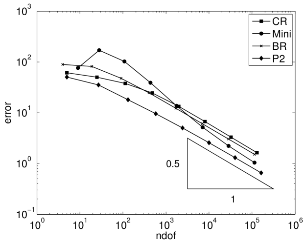
Figure 5.1: Convergence history for the colliding flow of Subsection 5.1.

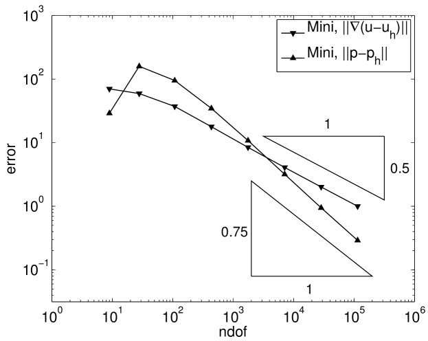
Figure 5.2: Convergence history for the pressure and velocity approximation of Mini-FEM for the colliding flow of Subsection 5.1.

Figure 5.1 shows that the MINI-FEM converges with an improved convergence rate in a pre-asymptotic range. This is due to the pressure approximation which converges with a rate of $-3/4$. This numerically highlights the result of Theorem 3.9 from [16] which was stated in Remark 4.10. Figure 5.2 clearly shows the difference of convergence rates for the pressure and velocity approximations. The pressure approximation converges with a rate of $-3/4$ whereas the velocity converges with a rate of $-1/2$ which also explains the overall convergence rate of $-1/2$ in the asymptotic regime.

5.2 L-shaped domain

On the L-shaped domain $\Omega=(-1,1)\times(-1,1)\setminus\left([0,1]\times[-1,0]\right)$ with right-hand side $f\equiv 0$, the exact solution, with the characteristic singularity at the origin, for the corresponding boundary conditions, reads

$$u(r,\vartheta) =\begin{pmatrix}r^{\alpha}((1+\alpha)\sin(\vartheta)w(\vartheta)+\cos(\vartheta)w_{\vartheta}(\vartheta))\\ r^{\alpha}(-(1+\alpha)\cos(\vartheta)w(\vartheta)+\sin(\vartheta)w_{\vartheta}(\vartheta))\end{pmatrix},$$

$$p(r,\vartheta) =-r^{\alpha-1}((1+\alpha)^{2}w_{\vartheta}(\vartheta)w_{\vartheta\vartheta\vartheta}(\vartheta))/(1-\alpha)$$

in polar coordinates with $\alpha=0.54448373$ and

$$w(\vartheta)= (\sin((1+\alpha)\vartheta)\cos(\alpha\omega))/(1+\alpha)-\cos((1+\alpha)\vartheta)$$

$$-(\sin((1-\alpha)\vartheta)\cos(\alpha\omega))/(1-\alpha)+\cos((1-\alpha)\vartheta).$$

Figure 5.3 shows the equivalence of all four FEMs also for this example with a reduced convergence rate of $-1/4$ with respect to the number of degrees of freedom.

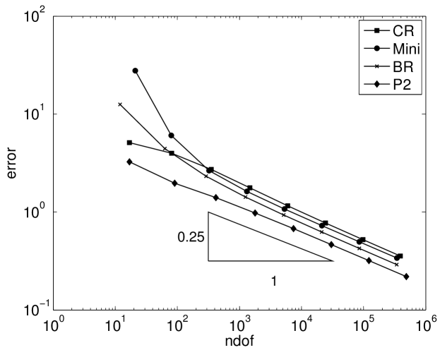
Figure 5.3: Convergence history for the L-shaped domain of Subsection 5.2.

5.3 Conclusions

The considered methods allow for comparison in one direction

$$\|\nabla(u-u_{\operatorname{P2}})\|+\|p-p_{\operatorname{P2}}\| \lesssim\|\nabla(u-u_{\operatorname{BR}})\|+\|p-p_{\operatorname{BR}}\|$$

$$\lesssim\|\nabla_{\operatorname{NC}}(u-u_{\operatorname{CR}})\|+\|p-p_{\operatorname{CR}}\|$$

$$\lesssim\|\nabla(u-u_{\operatorname{MINI}})\|+\|p-p_{\operatorname{MINI}}\|+\|h_{\mathcal{T}}f\|.$$

In typical situations, for example, if $p\not\equiv 0$, numerical experiments show, that all the methods (and also stabilised $P_{1}P_{0}$ , discontinuous Galerkin, and pseudostress FEMs) exhibit equivalent accuracy on a per-degree-of-freedom basis.

It is clear that this observation disregards other measures for the quality and performance of FEMs such as application-driven error functionals or even the effort of implementation. Other performance measures may lead to different assessments of the methods in practice.

6 Acknowledgements

This work is supported by the DFG Research Center Matheon Berlin and by the WCU program through KOSEF (R31-2008-000-10049-0). M. Schedensack is supported by the Berlin Mathematical School.

References

- [1] D. N. Arnold, F. Brezzi, and M. Fortin. A stable finite element for the Stokes equations. Calcolo, 21(4):337–344 (1985), 1984.
- [2] S. Badia, R. Codina, R. Gudi, and J. Guzmán. Error analysis of discontinuous Galerkin methods for Stokes problem under minimal regularity. IMA J. Numer. Anal., 2013. in press.
- [3] A. T. Barker and S. C. Brenner. A mixed finite element method for the Stokes equations based on a weakly over-penalized symmetric interior penalty approach. J. Sci. Comput., 2013.
- [4] C. Bernardi and G. Raugel. Analysis of some finite elements for the Stokes problem. Mathematics of Computation, 44(169):71–79, 1985.
- [5] Daniele Boffi, Franco Brezzi, Leszek F. Demkowicz, Ricardo G. Durán, Richard S. Falk, and Michel Fortin. Mixed finite elements, compatibility conditions, and applications, volume 1939 of Lecture Notes in Mathematics. Springer-Verlag, Berlin, 2008. Lectures given at the C.I.M.E. Summer School held in Cetraro, June 26–July 1, 2006, Edited by Boffi and Lucia Gastaldi.
- [6] Daniele Boffi, Franco Brezzi, and Michel Fortin. Mixed finite element methods and applications, volume 44 of Springer Series in Computational Mathematics. Springer, Heidelberg, 2013.
- [7] Dietrich Braess. An a posteriori error estimate and a comparison theorem for the nonconforming element. Calcolo, 46(2):149–155, 2009.
- [8] Susanne C. Brenner and L. Ridgway Scott. The mathematical theory of finite element methods, volume 15 of Texts in Applied Mathematics. Springer, New York, third edition, 2008.
- [9] C. Carstensen, D. Gallistl, and M. Schedensack. Adaptive nonconforming Crouzeix-Raviart FEM for eigenvalue problems. Math. Comp., 2013. (accepted for publication).
- [10] C. Carstensen, D. Peterseim, and M. Schedensack. Comparison results of finite element methods for the Poisson model problem. SIAM J. Numer. Anal., 50(6):2803–2823, 2012.
- [11] Carsten Carstensen, Dietmar Gallistl, and Mira Schedensack. Quasi-optimal adaptive pseudostress approximation of the Stokes equations. SIAM J. Numer. Anal., 51(3):1715–1734, 2013.
- [12] Carsten Carstensen, Dongho Kim, and Eun-Jae Park. A priori and a posteriori pseudostress-velocity mixed finite element error analysis for the Stokes problem. SIAM J. Numer. Anal., 49(6):2501–2523, 2011.
- [13] M. Crouzeix and P.-A. Raviart. Conforming and nonconforming finite element methods for solving the stationary Stokes equations. I. Rev. Française Automat. Informat. Recherche Opérationnelle Sér. Rouge, 7(R-3):33–75, 1973.
- [14] Enzo Dari, Ricardo Durán, and Claudio Padra. Error estimators for nonconforming finite element approximations of the Stokes problem. Math. Comp., 64(211):1017–1033, 1995.
- [15] Jim Douglas, Jr. and Jun Ping Wang. An absolutely stabilized finite element method for the Stokes problem. Math. Comp., 52(186):495–508, 1989.
- [16] Hagen Eichel, Lutz Tobiska, and Hehu Xie. Supercloseness and superconvergence of stabilized low-order finite element discretizations of the Stokes problem. Math. Comp., 80(274):697–722, 2011.
- [17] Thirupathi Gudi. A new error analysis for discontinuous finite element methods for linear elliptic problems. Math. Comp., 79(272):2169–2189, 2010.
- [18] Alessandro Russo. Bubble stabilization of finite element methods for the linearized incompressible Navier-Stokes equations. Comput. Methods Appl. Mech. Engrg., 132(3-4):335–343, 1996.
- [19] R. Verfürth. A posteriori error estimators for the Stokes equations. Numer. Math., 55(3):309–325, 1989.
- [20] R. Verfürth. A review of a posteriori estimation and adaptive mesh-refinement techniques. Advances in Numerical Mathematics. Wiley-Teubner, 1996.