Effects of the initial conditions on cosmological $N$-body simulations

Abstract

Cosmology is entering an era of percent level precision due to current large observational surveys. This precision in observation is now demanding more accuracy from numerical methods and cosmological simulations. In this paper, we study the accuracy of $N$-body numerical simulations and their dependence on changes in the initial conditions and in the simulation algorithms. For this purpose, we use a series of cosmological $N$-body simulations with varying initial conditions. We test the influence of the initial conditions, namely the pre-initial configuration (preIC), the order of the Lagrangian perturbation theory (LPT), and the initial redshift ($z_{\text{ini}}$), on the statistics associated with the large scale structures of the universe such as the halo mass function, the density power spectrum, and the maximal extent of the large scale structures. We find that glass or grid pre-initial conditions give similar results at $z\lesssim 2$. However, the initial excess of power in the glass initial conditions yields a subtle difference in the power spectra and the mass function at high redshifts. The LPT order used to generate the initial conditions of the simulations is found to play a crucial role. First-order LPT (1LPT) simulations underestimate the number of massive haloes with respect to second-order (2LPT) ones, typically by 2% at ${10^{14}}\,h^{-1}{M}_{\odot}$ for an initial redshift of 23, and the small-scale power with an underestimation of 6% near the Nyquist frequency for $z_{\text{ini}}={23}$. Larger underestimations are observed for lower starting redshifts. Moreover, at higher redshifts, the high-mass end of the mass function is significantly underestimated in 1LPT simulations. On the other hand, when the LPT order is fixed, the starting redshift has a systematic impact on the low-mass end of the halo mass function. Lower starting redshifts yield more low-mass haloes. Finally, we compare two $N$-body codes, Gadget-3 and GOTPM, and find 8% differences in the power spectrum at small scales and in the low-mass end of the halo mass function.

1 Introduction

Cosmological simulations have proved to be one of the most powerful tools for the study of the non-linear evolution of large-scale structures (LSS) of the Universe. In the hierarchical cold dark matter model with a cosmological constant ($\Lambda$CDM), structure formation occurs from bottom up, with the collapse of primordial density fluctuations forming low-mass haloes that later merge to form more massive ones (e.g. Blumenthal et al., 1984; Davis et al., 1985), while the rate and type of mergers are governed by the large-scale background environment (e.g. Hwang & Park, 2009; L’Huillier et al., 2014). The pioneering work of Press & Schechter (1974), later improved by more refined approaches, (e.g. Sheth & Tormen, 2002), provides us with important physical insights on the evolution of the large scale structures through the study of the halo mass function (e.g. Jenkins et al., 2001; Warren et al., 2006; Tinker et al., 2008).

Cosmology has entered an era of percent-level precision thanks to the recent high-resolution cosmic microwave background observations (Hinshaw et al., 2013; Planck Collaboration et al., 2013) and huge galaxy redshift surveys (e.g. 2dF, Colless 1999; BOSS, Dawson et al. 2013; DES). In concert with observational advancements, analytic perturbation theories have also been refined and can now describe the quasi-linear evolution of density fields to higher precision. However, comparing the results of numerical simulations to theoretical expectations is not an easy task. Because of the non-linear nature of structure formation, no theory can accurately predict the mass function or the non-linear part of the power spectrum. One has to rely on fits to cosmological simulations to model the halo mass function (e.g., Sheth & Tormen, 2002; Warren et al., 2006; Tinker et al., 2008) or the non-linear power spectrum (Smith et al., 2003) to study structure formation and to confront cosmological models to observations. In making accurate comparisons between models and observations, it is now necessary to know whether numerical simulation can yield convergent results, and to determine the simulation parameters to produce accurate results. Several studies reported that the results of a simulation are sensitive to the choice of the starting redshift (Lukić et al., 2007; Knebe et al., 2009; Heitmann et al., 2010; Reed et al., 2013), the order of the Lagrangian perturbation theory (Scoccimarro, 1998; Crocce et al., 2006, 2010; Jenkins, 2010), or the initial distribution of the particles prior to applying the displacement, namely on a regular lattice (grid), or a glass configuration (White, 1994; Wang & White, 2007). Lukić et al. (2007) claimed that the root mean square (rms) of the displacement should be small (typically 0.20 times the mean particle separation), and that the Nyquist frequency should be in the linear regime at the starting epoch. They also claimed that there should be at least about 10 expansion factors between $z_{\text{ini}}$ and the first redshift of interest so that the memory of the initial grid or glass configuration is lost. Knebe et al. (2009) inspected the influence of the starting redshift on the inner structure of haloes (triaxiality, spin parameter, and concentration), using both 1LPT and 2LPT. They found that starting redshift and LPT order have little influence on the internal halo properties. Initial conditions generated by 1LPT are known to produce transients, and 2LPT can be used to reduce the effects of these transients (Crocce et al., 2006).

The initial configuration should satisfy several requirements: the configuration should be isotropic, homogeneous, and should be in a state of equilibrium. The most popular preICs are regular lattice (grid) and glass, but several other configurations have also been introduced (e.g. quaquaversal tiling, Hansen et al., 2007). Setting the initial configuration of particles on a regular grid introduces preferred directions. Moreover, warm and hot dark matter simulations have shown unphysical features on the scale of the pixel size, suggesting that grid preICs are not well suited when structures form in a top-down way and the initial power of density fluctuation vanishes on the pixel scale. Some authors (e.g. White, 1994) advocate the use of more elaborated techniques like glass preICs. For this configuration, particles are randomly (uniformly) placed on a grid, then the set of particles is advanced by a repulsive gravitational force law until it reaches an equilibrium state where particles feel virtually no forces. However, the drawback of this technique is that reaching the equilibrium is computationally expensive, and one should test whether the configuration is indeed in a state of equilibrium. Another problem is that the density field started from glass preICs contains spurious clustering on small scales, which does not grow, but should be taken carefully into account, especially when one wants to study high-redshift physics.

Table 1: Simulations used in this study. Set 1 consists of GOTPM simulations, with the equivalent Gadget simulation for T2s, T3s and T4s. T3s and G3 have been run with 4 different realisations. Set 2 uses a WMAP7 cosmology with different random seeds.

ID	$N_{\text{p}}$	$L_{\mathrm{box}}$	$z_{\text{ini}}$	LPT	PreIC	r.m.s./$\Delta x$	Comments
		(${}\,h^{-1}\mathrm{Mpc}$)
Set 1:							GOTPM, WMAP5 cosmology
T2s	10243	256	100	2	mesh	0.47	Gadget-3 run: G2s
T3s	15123	256	100	2	mesh	0.26	4 realisations; Gadget-3 run: G3s
T3f	15123	256	100	1	mesh	0.26	4 realisations
T4s	15123	256	50	2	mesh	0.51	4 realisations; Gadget-3 run: G4s
T4f	15123	256	50	1	mesh	0.51	4 realisations
T5s	15123	256	23	2	mesh	1.09	4 realisations
T5f	15123	256	23	1	mesh	1.09	4 realisations
T7s	15123	768	100	2	mesh	0.089
T8s	15123	768	50	2	mesh	0.18
T9s	15123	768	23	2	mesh	0.38
Set 2:							Gadget-3, WMAP5 glass/mesh
G3sm	15123	256	100	2	mesh
G3sg	15123	256	100	2	glass
G4sm	15123	256	50	2	mesh		4 realisations
G4sg	15123	256	50	2	glass		4 realisations
Set 3:							Gadget-3, WMAP7
G7s	15123	768	50	2	mesh
G7f	15123	768	50	1	mesh
G8s	15123	768	23	2	mesh
G8f	15123	768	23	1	mesh

In the last few years several authors have begun to investigate the possibility of percent level accuracy of the power spectrum (PS) and halo mass function (MF) in numerical simulations (Heitmann et al., 2010; Reed et al., 2013). Heitmann et al. (2010) used a high $z_{\text{ini}}$ and 1LPT rather than a lower initial redshift with 2LPT, arguing that higher initial redshift yields convergence in the mass function at $z=0$ and is not computationally expensive. However, Reed et al. (2013) found that too high a starting redshift ($z_{\text{ini}}\gtrsim 200$ for a mean particle separation of ${2}\,h^{-1}\mathrm{Mpc}$) produces an erroneous mass function because the amplitude of the initial fluctuations is too low compared to the level of numerical noise. They claim that 2LPT, with at least 10-50 expansion factors before the first redshift of interest, should be used. Moreover, they studied the influence of several parameters of Tree codes on the halo mass function, and the power spectrum.

The aim of this paper is to study the effect of changes in the initial conditions at fixed cosmology on the large-scale structure statistics. To do so, we quantify the influence of the preICs, the LPT order, and the starting redshift on large-scale statistics such as the density power spectrum, the halo mass function, and the distribution of the size of structures. Since we aim to study the effects of the initial conditions on the properties of large-scale structures (LSS), the individual properties of haloes are not studied in this paper.

Section 2 presents the set of simulations we used in this work. Section 3 presents the statistics that we used for the analysis. Our main results are shown in § 4, and our conclusions are drawn in § 5. A aims to find the best estimation of the power spectrum.

2 Simulations

2.1 Initial Conditions

The comoving positions of particles in the initial conditions is computed via

$$\mathbf{x}(\tau)=\mathbf{q}+\mathbf{\Psi}(\mathbf{q},\tau),$$ (1)

where $\mathrm{d}\tau=\mathrm{d}a(t)/a(t)$ is the conformal time, $\mathbf{x}$ is the Eulerian (after displacement) position, $\mathbf{q}$ the Lagrangian (initial) position, and $\mathbf{\Psi}$ the displacement field. Here, $\mathbf{x}$ obeys the equation

$$\frac{\mathrm{d}{{}^{2}\mathbf{x}}}{\mathrm{d}{\tau^{2}}}+\mathcal{H}(\tau)\frac{\mathrm{d}{\mathbf{x}}}{\mathrm{d}{\tau}}=-\mathbf{\nabla\phi},$$ (2)

where $\phi$ is the potential field, and $\mathcal{H}=aH$. The displacement field $\mathbf{\Psi}$ is given to the second order by

$$\mathbf{\Psi}(\mathbf{q},\tau)=-D_{1}(a)\mathbf{\nabla}_{q}\phi^{(1)}(\mathbf{q})+D_{2}(a)\mathbf{\nabla}_{q}\phi^{(2)}(\mathbf{q}),$$ (3)

where the $D_{i}$ are the first- and second-order growth factors, and $\phi^{(i)}$ are the first- and second-order potentials. The first order approximation, which assumes $\mathbf{\nabla}\phi^{(2)}=0$, is called the Zel’dovich approximation.

The initial conditions for our first set of simulations were generated by the IC generator included in GOTPM, which is able to generate both 1LPT and 2LPT ICs, using a CAMB input power spectrum at $z=0$. The ICs for the second and third sets of simulations were generated using the 2LPTic code described in Crocce et al. (2006).

2.2 Sets of simulations

Our simulations used a WMAP5 cosmology (sets 1 and 2) with $(\Omega_{\text{b}},\Omega_{\text{m}},\Omega_{\Lambda},h,\sigma_{8},n_{s})$ = (0.044, 0.26, 0.74, 0.72, 0.79, 0.96), and set 3 used a WMAP7 cosmology (0.0455, 0.272, 0.728, 0.702, 0.807, 0.961). The simulation parameters are summarised in Table 1. Our reference set of simulations uses the GOTPM code (Dubinski et al., 2004; Park et al., 2005a). GOTPM has long been used to run cosmological simulations (Park et al., 2005b), including the recent Horizon runs (Kim et al., 2009, 2011). This TreePM code is the merger of the PM code of Park (1990) and the Tree code of Dubinski (1996). A second set of simulations was run using the TreePM-SPH Gadget-3 code, an enhanced version of the public Gadget-2 code (Springel, 2005).

Hereafter, we will refer to the simulations using their names in the table, and to groups of simulations with their common features (number of particles $N$, order of LPT, preIC, initial redshift, or box size). Our choice of the softening parameter ($\varepsilon_{\text{soft}}=0.1\bar{d}$) is slightly above the recommended value of Reed et al. (2013). The size of the PM grid was set equal to the number of particles in each dimension, in both Gadget and GOTPM runs.

Rather than running several identical simulations with different random seeds, we chose to use the same random seed, thus allowing us to observe the variation of the initial parameters free from statistical fluctuations. However, this introduces a bias while comparing simulations with different resolutions due to the random fluctuations in the initial conditions. In order to alleviate this issue, we ran three additional T3, T4, T5 1LPT and 2LPT simulations, and the corresponding G3, G4, and G5 simulations that we used for the comparison of Gadget and GOTPM.

3 Statistics

3.1 Power spectrum

The matter density power spectrum is defined as

$$P(k)=\frac{1}{V}\left\langle\left\lvert\delta(\mathbf{k})\right\rvert^{2}\right\rangle,$$ (4)

where $V$ is the volume on which it is computed, and $\delta(\mathbf{k})$ is the Fourier transform of the overdensity field defined as $\delta(\mathbf{x})=\rho(\mathbf{x})/\bar{\rho}-1$.

Jing (2005) found a formula to remove the windowing effects from the PS that arise due to mass assignment schemes. They showed that the raw power spectrum $\left\langle\left\lvert\delta^{f}(\mathbf{k})\right\rvert^{2}\right\rangle$ measured from the simulation using a fast Fourier transform (FFT) is related to the real power spectrum $P(\mathbf{k})$ via

$$\left\langle\left\lvert\delta^{f}(\mathbf{k})\right\rvert^{2}\right\rangle =\sum_{\mathbf{n}\in\mathbb{Z}^{3}}\left\lvert W(\mathbf{k}+2k_{\mathrm{N}}\mathbf{n})\right\rvert^{2}P(\mathbf{k}+2k_{\mathrm{N}}\mathbf{n})$$

$$+\frac{1}{N}_{\text{p}}\left\lvert W(\mathbf{k}+2k_{\mathrm{N}}\mathbf{n})\right\rvert^{2},$$ (5)

where $k_{\text{N}}={N_{\text{p}}\pi}/L$ is the Nyquist frequency, the first term in the second hand of the equation is the effect of aliasing and the convolution by the window function $W$ owing to the mass assignment scheme, and the second term is the Poisson shot noise. Another way to deal with this aliasing effect is to optimise the choice of the window function (Cui et al., 2008). Colombi et al. (2009) introduced a Taylor-Fourier transform to accurately measure the power spectrum.

The estimation of the power spectrum is discussed in A. We use a triangular shaped cloud (TSC) mass assignment scheme, using $N_{\text{grid}}^{3}=2^{3}N_{\text{p}}^{3}$, and corrected for pixelation effect. However we do not correct for shot noise nor aliasing. Finally, we use a cloud-in-cell (CIC) scheme to bin the modes into linearly spaced bins of $2\pi/L$.

3.2 Mass function

Haloes were detected at $z=0$ using a friends-of-friends (FOF) algorithm. FOF links together particles with a separation smaller than $b$ times the mean interparticle distance, where $b$ is the so-called linking length parameter. Usually, a value of $b=0.2$ is chosen since it has been shown to reproduce fairly accurately the abundance of virialised haloes (eg, Lacey & Cole, 1994). We computed the mass function of FOF haloes with more than or equal to 20 particles for each simulation, yielding a mass threshold of ${1.8\times 10^{11}}\,h^{-1}{M}_{\odot}$ for the simulations with $512^{3}$ particles and a box size of ${256}\,h^{-1}\mathrm{Mpc}$ (e.g. T3, T4, T5). While 20 particles is definitely not enough to obtain robust results on the internal properties of low-mass haloes, since we are interested in the differences in the mass function, this issue should not be too important here.

The mass of a halo is not well defined in simulations. We use here the FOF mass, that is the sum of the masses of particles composing the halo. We used the canonical value $b=0.2$ for the linking length parameter, which yields haloes with isodensity contours of $\approx 75$ times the critical density (Lukić et al., 2009). The boundaries of the FOF haloes can have complex geometry but are well-defined in terms of the local density (they are isodensity surfaces). The FOF halo finding algorithm is the most commonly used method for estimation of the halo mass function in cosmological simulations (eg Jenkins et al., 2001; Warren et al., 2006). Its results are known to differ from Spherical Overdensity halo masses (cf Lukić et al., 2009; More et al., 2011, for example). We chose to use FOF haloes because SO by definition only finds spherical haloes, while FOF can deal with more complex geometries.

3.3 Size of the large scale structures

In addition to the power spectrum and the halo mass function, which have been used in previous studies, we also studied connectivity of the LSS. We identified the LSS in our simulations using the method proposed by Park et al. (2012). We applied the FOF algorithm to the halo catalogue, in order to group them. This is a robust and simulation-independent way to define the large scale structures. We varied $b$ from 0.2 to 0.8, with a step of 0.025, to find the value $b_{\text{max}}$ that maximises the number of structures. A low value of $b$, corresponding to a high density threshold, will produce many small objects, while a large value (low threshold) will produce few very large ones. Interestingly, for all these simulations, we found a value of $b_{\text{max}}$ between 0.5 and 0.55. To detect the subtle dependence of LSS on the choice of initial conditions, we fixed the linking length to $b=0.55$ to identify the LSS in all simulations. The mean halo separations are 3.92 and ${4.02}\,h^{-1}\mathrm{Mpc}$ for T3s and T7s. For each of these large scale structures, we computed the maximal extent $l_{\text{max}}$, which is the maximal distance between each pair of haloes within the structure, and study the cumulative distribution of the maximal extent. In the higher resolution simulations, T2s and G2s, the analysis was made using only haloes that can be resolved in the lower resolution simulations, namely, $M_{\text{min}}={1.80\times 10^{11}}\,h^{-1}{M}_{\odot}$, so that we effectively study the same kind of objects in different simulations.

4 Results

In this section we present the main results of our study on the effects of the preIC, the order of perturbation theory, the starting redshift, and the effect of the $N$-body code. We use statistics such as the power spectrum, the halo mass function, and the distribution of the maximal extent of the LSS. Our results should be taken with caution because the magnitude of the effects presented below depends on the resolution of the simulations. In most cases, we are using simulations with mean particle separations of 0.5 and ${1.5}\,h^{-1}\mathrm{Mpc}$.

4.1 Pre-initial configuration

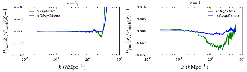
Figure 1: Effects of the preICs on the power spectrum. Shown are the power spectra of the glass simulation divided by those of the grid ones for G3sg and G3sm (green), and the average of the four G4sg and G4sm.

The first variable that we investigated is that of the pre-initial configuration, which took the form of either a glass or a regular mesh. Figure 1 shows the power spectra of the glass simulations divided by that of the corresponding mesh simulations, at initial (left) and final (right) redshifts, for the G3sg/G3sm (green) and G4sg/G4sm (blue) simulations. In the G4sg and G4sm cases, we took the average over the 4 realisations. At the initial epoch, the agreement is about $0.1\%$ until $k\approx{3}\,h\,\mathrm{Mpc}^{-1}$, and the power of glass-preICs steeply rises for very high $k$. The power spectrum is misrepresented up to a few pixel scales in the case of the glass preIC. At $z=0$, the agreement is better than our desired level of 1% at all scales. The initial excess of power on small scales has been overtaken by the power produced by the gravitational clustering. We note that the difference between glass and mesh preICs is larger in the G3sg/G3sm ($z_{\text{ini}}=100$) than the G4sg/G4sm ($z_{\text{ini}}=50$) case. This is still true when we only consider the first run of G4sg and G4sm, which shares the same random seed as the G3sg/G3sm run.

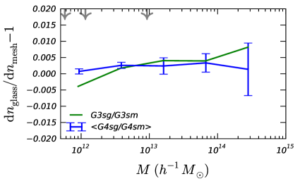
Figure 2: Effects of the preICs on the halo mass function. Shown are the mass functions of the glass simulation divided by those of the grid ones for G3sg and G3sm (green), and the average of the four G4sg and G4sm (blue). The grey arrows show the mass of 64, 128, and 1024 particles.

Figure 2 shows the mass function at $z=0$ of the glass versus grid preIC simulations, averaged over the four realisations in the case of G4sg/G4sm. The error bar is the standard deviation in each bin, showing the variations among the four runs. The grey arrows show the mass of 64, 128, and 1024 particles. At all masses, glass and grid simulations agree to better than 1%. Figure 3 shows the effects of the preICs on the size distribution of LSS. It shows the ratio of the cumulative distributions $n(>L_{\text{max}})$ of the glass and grid simulations. The error bars are now much larger, up to 15%, due to the relatively small simulation box size, but the glass and grid simulations agree within these error bars.

Even though the initial power spectra are different, the final results seem to be consistent with each other. One may then wonder when these differences are washed out by the non-linear gravitational evolution. Figure 4 shows the evolution of the ratio of the glass to grid power spectra, averaged over the four G4sm and G4sg simulations. At $z=3$, when the scale factor increased by a factor of about 13, the difference is already smaller than 1%, and becomes smaller than 0.2% at $z=2$. Interestingly, at $z=3$, the glass simulation show less small scale power than the grid case. This reflects the fact that non-linear evolution occurs later in the glass case. Figure 5 shows the ratios of the halo mass functions of the four G4sm and G4sg simulations at different redshifts. Up to $z=2$, the mass functions agree within a few percent. At $z=3$, the number density of low-mass haloes ($M<{10^{13}}\,h^{-1}{M}_{\odot}$) is underpredicted in the glass simulations with respect to the grid one, which is consistent with the power spectrum results.

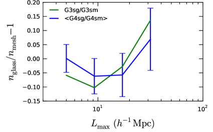
Figure 3: Effects of the preICs on the size distribution of the large-scale structures, same legend as Fig. 2.

4.2 Order of perturbation theory

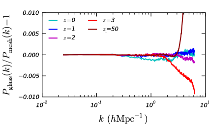
Figure 4: Redshift evolution of ratio of the glass to grid power spectra averaged over the four G4sm and G4sg simulations.

Figure 6 shows the effects of the LPT order on the power spectrum at the initial (left) and final (right) epochs, for different simulations. The initial redshifts are 100 for T3 and G7, 50 for T4 and G8, and 23 for T5. The T (G)simulations were run in a ${256\,(768)}\,h^{-1}\mathrm{Mpc}$ box. The power spectra of T3, T4, and T5 were averaged over the four realisations. At the initial epoch, the 1LPT ICs show a lack of small-scale power, which increases when the initial redshift decreases. At initial redshifts of 100 and 50, the initial power between 1 and 2LPT agree to better than 1% on all scales, while at initial redshift of 23, the difference reaches 2% at small scales ($\approx{5}\,h\,\mathrm{Mpc}^{-1}$). This is expected from Lagrangian perturbation theory, because 1LPT and 2LPT should converge towards high starting redshifts. At $z=0$, for the $z_{\text{ini}}={100}$ simulations, the power spectra of the 1LPT and 2LPT simulations agree to better than 2% on all scales. This agreement is good on scales of $k\leq{0.2\,(0.15)}\,h\,\mathrm{Mpc}^{-1}$ for a starting redshift of 50 (23). The critical value of $k$ where the agreement ceases to be valid is independent of the box size, as shown by the G simulations, and only depends on the initial redshift. Even when the initial agreement in the power spectrum is better than 1% on all scales, as in the $z_{\text{ini}}={50}$ case, the final power spectra can differ by 2–3%. This can be understood because the use of 1LPT or 2LPT not only affects the initial displacement, but also the initial velocity. Therefore, an initial agreement of 1% is not a sufficient condition to get an accuracy of 1% at $z=0$ in the power spectrum.

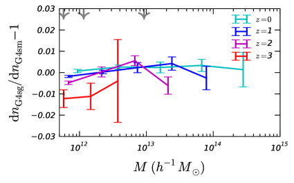
Figure 5: Redshift evolution of ratio of the glass to grid halo mass function averaged over the four G4sm and G4sg simulations. The grey arrows show the mass of 64, 128, and 1024 particles.

Figure 7 shows the influence of the LPT order on the mass function at $z=0$, averaged over four realisations for the T3, T4, and T5 sets of simulations. For the $z_{\text{ini}}={100}$ case, the agreement between 1LPT and 2LPT is within the error bars. At low masses, $M\lesssim{2\times 10^{13}}\,h^{-1}{M}_{\odot}$, the agreement is within 1% in all simulations, but at higher masses, the mass function is slightly lower in the case of 1LPT, up to 3% at $M\simeq{10^{14}}\,h^{-1}{M}_{\odot}$ for the $z_{\text{ini}}={23}$ case. Figure 8 shows the effects of the LPT order on the LSS. At all starting redshifts, the 1 and 2LPT simulations yield similar results.

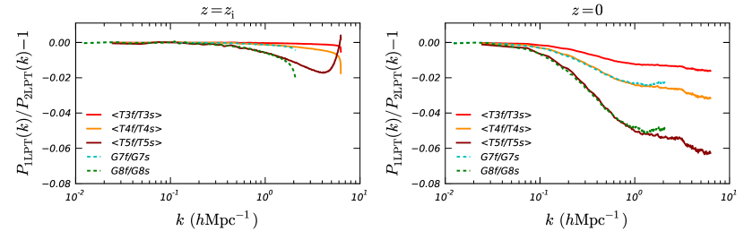
Figure 6: Influence of the LPT order on the power spectrum at $z=z_{\text{ini}}$ (left) and $z=0$ (right). Shown are the ratios of the 1LPT to 2LPT simulations for starting redshifts of 100 (T3), 50 (G7 and T4), and 23 (G8 and T5), averaged over four realisations in the case of T3, T4, and T5.

Here again, it is interesting to study how these relations evolve in time (McBride et al, private communication). Figure 9 shows the time evolution of the ratio of the mass functions of the T3f and T3s simulations ($z_{\text{ini}}={100}$), averaged over 4 realisations, at $z=0$ (cyan), 1 (blue), 2 (magenta), and 4 (red). At redshifts $z>0$, the 1LPT always underestimates the mass function with respect to 2LPT. At $z=0$, as seen in Fig. 7, they are consistent with each other. However, with increasing redshift, the 1LPT simulation underestimates the mass function. At $z=1$, the underestimation is up to 5% at $M\simeq{10^{14}}\,h^{-1}{M}_{\odot}$. At $z=2$, the underestimation is close to 5% for haloes with mass of ${10^{13}}\,h^{-1}{M}_{\odot}$, and larger than 1% at all mass. At $z=4$, the underestimation is greater than 10% above ${10^{12}}\,h^{-1}{M}_{\odot}$. If we want to produce the halo mass function on the mass scale and below ${10^{13}}\,h^{-1}{M}_{\odot}$ more accurately than 1%, from 1LPT simulations, only data after $z=1$, or with more than 50 expansion factors, should be used.

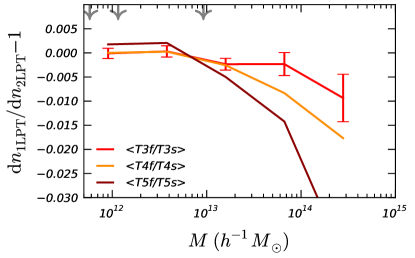
Figure 7: Influence of the LPT order on the halo mass function, same legend as Fig. 6.

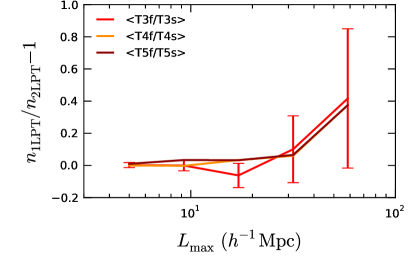
Figure 8: Influence of the LPT order on the distribution of the maximal extent of the LSS, same legend as Fig. 6.

4.3 Initial redshift

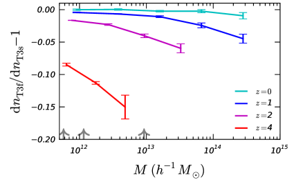
Figure 9: Evolution of the 1LPT versus 2LPT mass function for the T4 (initial redshift of 50) simulations.

In this section we focus on how the choice of starting redshift effects the simulation at $z=0$. This question has been raised in several previous studies (eg, Lukić et al., 2007; Knebe et al., 2009; Heitmann et al., 2010; Reed et al., 2013). However for completeness we also investigate this issue within our suite of simulations. We will restrict ourselves to the study of the 2LPT case, since we already focused on the role of the LPT order in the previous section. Using too high a starting redshift causes the displacement to be small with respect to the length resolution, yielding inaccurate initial conditions. On the other hand, starting too late may break the validity of the approximation used for the initial perturbations. We reported the rms of the initial displacement in Table 1 in units of the mean particle separation. The T3 simulations have a reasonable value, 0.26, and T4 have a slightly high value, 0.51. The T5 simulations have a rms displacement of 1.09, which is slightly larger than the mean separation. We note that, while this value is high, it does not imply that shell crossing has occurred, since displacements are correlated. On the other hand, in the ${768}\,h^{-1}\mathrm{Mpc}$ box, T7s ($z_{\text{ini}}={100}$) has a low value, 0.089, while those of T8s ($z_{\text{ini}}={10}$) and T9s ($z_{\text{ini}}={23}$) are more reasonable, therefore, we might expect the results of T8s and T9s to be more accurate. However, we still use T7s as the reference simulation in the large box in order to be consistent.

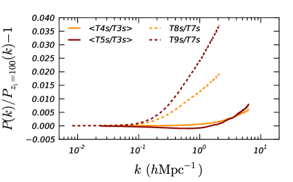
Figure 10: Influence of the initial redshift on the power spectrum, 2LPT. The solid lines show the ${256}\,h^{-1}\mathrm{Mpc}$ box, averaged over 4 runs, and the dashed lines, the ${768}\,h^{-1}\mathrm{Mpc}$ one.

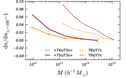
Figure 11: Influence of the initial redshift on the halo mass function. Same legend as Fig. 10

Fig. 10 shows the power spectra of T4s and T5s divided by that of T3s, and averaged over 4 realisations. Also shown are the power spectra of T8s, and T9s, divided by T7s. On large scales, the power spectra agree exactly, and start to deviate when approaching the Nyquist frequency. For the ${256}\,h^{-1}\mathrm{Mpc}$ simulations, the agreement is better than 1% on all scales. The deviation is slightly larger in the ${768}\,h^{-1}\mathrm{Mpc}$ box, where it reaches 3.5%. However, we must keep in mind that the power spectrum of T7s might not be accurate, owing to the small initial displacement. Figure 11 shows the effects of the starting redshift on the halo mass function at $z=0$. Shown are the mass functions of T4s and T5s divided by that of T3s, and T8s, and T9s, divided by that of T7s. On large masses, in the small box case, all simulations agree, but when going toward low masses ($<{10^{13}}\,h^{-1}{M}_{\odot}$), a clear effect of the starting redshift can be seen. Simulations with a lower starting redshift overestimate the number density of low-mass haloes by up to 4% (T4s) and 8% (T5s). For the larger box, the results is even more striking. At $M\simeq{10^{15}}\,h^{-1}{M}_{\odot}$, the three simulations agree, but at lower masses the differences appear, up to 10% at $M\simeq{10^{13}}\,h^{-1}{M}_{\odot}$ for the T9s case.

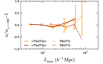
Figure 12: Influence of the initial redshift on the maximal extent of LSS, same legend as 10.

Figure 12 shows the effects of the starting redshift on the distribution of the LSS. At the small-size end of the distribution, all simulations agree very well. On larger sizes, the uncertainty becomes more important. To the accuracy reached by the simulations, no significant difference can be seen between the different simulations. If we combine this result with that in the previous section, it can be said that the size distribution of LSS estimated from simulations with a relatively low initial redshift and 1LPT ICs is reliable (i.e. Park et al. 2012 who used $z_{\text{ini}}={32}$, 1LPT, and a mean particle separation of ${1.2}\,h^{-1}\mathrm{Mpc}$).

4.4 $N$-body code comparison: GOTPM versus Gadget-3

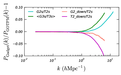
Figure 13: Influence of the $N$body code on the power spectrum. Shown are the power spectra of Gadget simulations divided by the corresponding GOTPM one. The G3s/T3s results were averaged over the four runs. A downsampled version of the G2s and T2s simulations, T2s_down and G2s_down, are also shown in magenta and salmon.

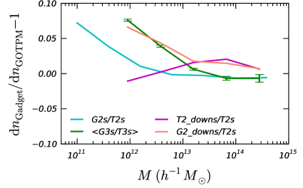
Figure 14: Influence of the $N$body code on the halo mass function. Same legend as Fig. 13

In this section, we compare the two cosmological codes. In order to test the consistency between GOTPM and Gadget, some simulations, namely T2s, T3s, and the first run of T4s (T4s Run 1), were also run using Gadget-3.

Figure 13 shows the power spectra of the Gadget simulations divided by those of the corresponding GOTPM ones. On large scales, the Gadget-3 and GOTPM simulations agree very well. However, on small scales $k>k_{\text{Ny}}/4$, the Gadget-3 simulation start to show an excess of power with respect to the corresponding GOTPM simulation, up to 8% at the Nyquist frequency. This effect is more important than the effects of the starting redshift. To better understand this difference, we also run a downsampled version of the T2s simulation with $512^{3}$ particles using GOTPM (T2s_down) and Gadget (G2s_down). In these simulations, the large-scale initial power is the same as the T2s simulation, which has 1024³ particles, but the initial density field has been binned down to $512^{3}$, losing the small-scale power information. The ratio of T2s_down and G2s_down to T2s are shown in salmon and magenta. The large-scale power agree exactly, as expected, and differences occur on small scales. T2s_down shows some lack of small-scale power at $k>{1}\,h\,\mathrm{Mpc}^{-1}$. In the case of G2s_down, the lack of small-scale power is balanced by the extra power of the Gadget runs, yielding a smaller difference.

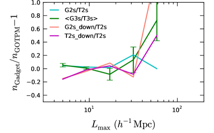
Figure 15: Influence of the $N$-body code on the size distribution of the large-scale structures. Same legend as Fig. 13

Figure 14 shows the ratio of the mass function of Gadget and GOTPM simulations The agreement is very good, with 1% accuracy at high masses. At fixed resolution, at high masses, the agreement is very good, better than 1%. However, at low masses, $M<{10^{13}}\,h^{-1}{M}_{\odot}$, Gadget overestimates the mass function with respect to GOTPM, up to 8%. The two downsampled simulations show an interesting feature. The high-mass end of the mass function ($M>{10^{13}}\,h^{-1}{M}_{\odot}$) is 2% higher than the T2s one. However, on low masses, they show different behaviours. G3s_down shows the same characteristics as the other Gadget runs, with an excess of low-mass haloes compared to T2s, while T2s_down shows closer results to T2s. It should be noted that G2s, the higher-resolution simulation with Gadget, agrees with T2s down to ${10^{12}}\,h^{-1}{M}_{\odot}$ to better than 2%. The fact that T2_down approaches both T2s and G2s near ${10^{12}}\,h^{-1}{M}_{\odot}$ while G2s_down deviates from them, means that Gadget is overproducing the haloes on small-mass scales.

Finally, Fig. 15 shows the effect of the $N$-body code on the size distribution of the LSS. No clear effect can be seen beyond the fluctuations.

5 Discussion and conclusion

We have created a suite of $N$-body simulations, run with various initial conditions that explored changes in the LPT order, the initial redshift, and the pre-initial configuration. This simulation dataset was used to quantify the sensitivity of observable statistics, such as the density power spectrum, the halo mass function, and the distribution of the LSS extent, on the numerical parameters. Our main findings are:

• We found that the choice of the pre-initial conditions does not affect the simulation results significantly: the difference is less than 1% for the power spectrum and the halo mass function. However, it should be pointed out that the density fluctuations are spuriously very high on small scales (up to twice the mean particle separation) due to the initial white noise power. Even though this power does not grow gravitationally, the excess persists until it is exceeded by the growing “true” power. This manifests itself most significantly at higher redshift where numerical artefacts may be confused with small-scale physics. At $z=3$, we found a lack of small-scale power and small-mass haloes in the glass simulations. However, after $z=2$ we found no statistical evidence for a systematic difference between the halo mass functions of the glass and mesh preIC simulations.

• One drawback in glass preICs is that choosing too high a starting redshift introduces larger errors compared to the lower starting redshift case. This may be because of the difficulty in realising the small-amplitude density fluctuations by a particle distribution with a white noise power. The interpolation of the initial displacement field from the mesh points to particle positions can be another source of errors.

• We confirmed that the 1LPT underestimates the power spectrum on small scales compared to the 2LPT simulations and that the differences increase as the starting redshift decreases. The halo mass function is slightly underestimated on the highest mass scales probed ($\simeq{10^{14}}\,h^{-1}{M}_{\odot}$) in the 1LPT case. The difference is approximately 1% near the mass scale of ${10^{14}}\,h^{-1}{M}_{\odot}$ when the starting redshift is 50, and the trend increases for lower starting redshifts. We find no statistically significant effect on the order of the LPT on the size distributions of LSS.

• We found that the underestimation in the mass function in the 1LPT simulations increases at high redshift. For an initial redshift of 100, it is less than 1% at $z=0$ and 1, about 5% at $z=2$, and more than 20% at $z=4$ on the mass scale of ${10^{13}}\,h^{-1}{M}_{\odot}$.

• We found that the starting redshift makes a systematic and statistically significant impact on the FOF halo mass function at small masses ($<{10^{13}}\,h^{-1}{M}_{\odot}$). The choice of relatively low starting redshifts ($z=50$ and 23 compared to 100) yielded an over-estimation of the mass function by a factor of more than 5% near the mass scale of ${10^{12}}\,h^{-1}{M}_{\odot}$. We do not find significant differences in the PS and the LSS size distribution for different starting redshifts.

• We compared the gravitational N-body integration codes GOTPM and Gadget on cosmologically significant scales. Both codes yield similar large-scale power spectra and high-mass mass functions, but it is found that Gadget overproduces the small mass haloes on the mass scale below about $10^{3}$ simulation particles. The overproduction reaches about 8% at a mass scale of $100$ particles.

Our results using 2LPT agree with previous studies (Heitmann et al., 2010; Reed et al., 2013), and here we stressed again the need for the use of 2LPT. We agree with Reed et al. (2013) about the need for 2LPT ICs, especially if one is interested in the high-redshift ($z\gtrsim 3$) mass function, where 1LPT ICs underestimate it more seriously. However, Reed et al. (2013) warned about false convergence in high starting redshift simulations. Before running $N$-body simulations, such tests should always be performed. In addition to the power spectrum and the halo mass function, which have been extensively studied before, the use of a new statistics, namely the size distribution of LSSs, provides us with information on the large scale.

In this study we have ignored hydrodynamical effects. While the large-scale evolution is predominately driven by gravity, on smaller scales the role of the baryons plays a more important but complicated role (e.g. Jing et al., 2006; Rudd et al., 2008; van Daalen et al., 2011; Cui et al., 2012; Hwang et al., 2013). Cui et al. (2012) showed that, even in a purely adiabatic case (i.e., no cooling nor star formation), the halo mass function may change up to $\approx 7\%$ for an overdensity of 500, showing the impact of the baryons in the inner parts of the haloes. In a next paper, we will extend the statistical tests presented here to cosmological hydrodynamical simulations.

Here we chose to study the convergence of simulation results for different numerical setups. Once simulations with a given cosmolgy can achieve 1% precision in the mass function, it becomes possible to test different cosmologies. Studying the cosmology dependence of the mass function is also a very important topic. For instance, Courtin et al. (2011) showed that the mass function is close to universal for cosmologies with close expansion histories, but deviates from universality for other cosmologies (Dark Energy).

Figure 9 shows that there is a few percent difference in the mass function between 1LPT and 2LPT at each redshift interval. The effects of other simulation setups on the mass function are smaller. On the other hand, Lundgren et al. (2014) find the mass function evolves by a factor of a few across similar redshift intervals. Therefore, the effect of evolution dominates the changes in the amplitude and shape of the mass function. At a given redshift, the uncertainties in the current observational data are still too large compared to the numerical uncertainties found in our paper. However, when the size of observations is increased, it will be necessary to have an accurate theoretical mass function that can be compared with the more accurately determined observed mass function in order to constrain cosmology and astrophysics.

Appendix A Power spectrum estimation

Our code for computing the power spectrum is based on the fastest Fourier transform in the west (FFTW) library. The density is evaluated on a user-defined grid (we chose $N_{\text{g}}=2^{3}N_{\text{p}}$), using either a nearest grid point (NGP), CIC, or TSC assignment scheme (Hockney & Eastwood, 1981). The modes are binned using a cloud-in-cell scheme assignment to attenuate the large-scales fluctuations due to the small number of modes in the first bins. The code is publicly available, is MPI-parallel, is able to read Gadget-3 and GOTPM snapshot files, and has been tested using up to a 4096³ grid on 96 MPI tasks. Figure 16 shows the initial power spectrum of the T3s simulation, normalised by the input linear power spectrum, and computed on several grid sizes and using different schemes, that are the cloud-in-cell (CIC, dashed lines), and triangular shape cloud (TSC, solid lines) mass scheme assignment, using a grid with a number of cells per dimension of 1024 (blue), and 512 (green). At fixed resolution, the TSC yields more accurate results than the CIC. The TSC, 1024 yields a measurement to 2% accuracy on all scales. This setting corresponds to with $N_{\text{grid}}^{3}=2^{3}N_{\text{p}}^{3}$, which we will keep for all measurements of the power spectrum in this paper. Note that Heitmann et al. (2010) also used the same setting, however using a CIC scheme.

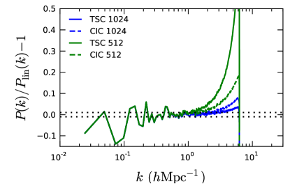
Figure 16: Power spectrum of a simulation (T3s) at the initial epoch $z=100$, with $N_{\text{grid}}=$ 512 (green), and 1024 (blue); computed with the CIC (dashed), and TSC (solid) schemes

Appendix B Effect of the halo-finder

It is beyond the scope of this article to study the convergence or disagreements among different halo finders. Knebe et al. (2011) performed such a comparison. In figure 17, we compare the mass function of the G4sm and G4sg simulations calculated by our FOF algorithm, AdaptaHOP (Aubert et al., 2004; Tweed et al., 2009) and AMIGA’s halo finder (AHF, Gill et al., 2004; Knollmann & Knebe, 2009). AdaptaHOP and AHF are subhalo finders, but the subhalo detection can be omitted and we only consider the main haloes in order to compare to the FOF haloes.

From Fig. 17, it is clear that, although the mass functions of FOF, AHF, and AdaptaHOP haloes are slightly different, the halo finder does not play an important role. The three halo finders agree within the error bars, except in the smallest mass bin for AHF, and the agreement is below the 1% level. We do not see systematic differences compared to the FOF case, so we conclude that this is rather insensitive to the halo finder.

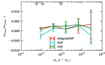
Figure 17: Comparison of the FOF, AdaptaHOP, and AHF mass functions for the G4sm anfd G3sg simulations.

References

- Aubert et al. (2004) Aubert, D., Pichon, C., & Colombi, S. 2004, MNRAS, 352, 376
- Blumenthal et al. (1984) Blumenthal, G. R., Faber, S. M., Primack, J. R., & Rees, M. J. 1984, Nature, 311, 517
- Colless (1999) Colless, M. 1999, Royal Society of London Philosophical Transactions Series A, 357, 105
- Colombi et al. (2009) Colombi, S., Jaffe, A., Novikov, D., & Pichon, C. 2009, MNRAS, 393, 511
- Courtin et al. (2011) Courtin, J., Rasera, Y., Alimi, J.-M., et al. 2011, MNRAS, 410, 1911
- Crocce et al. (2010) Crocce, M., Fosalba, P., Castander, F. J., & Gaztañaga, E. 2010, MNRAS, 403, 1353
- Crocce et al. (2006) Crocce, M., Pueblas, S., & Scoccimarro, R. 2006, MNRAS, 373, 369
- Cui et al. (2012) Cui, W., Borgani, S., Dolag, K., Murante, G., & Tornatore, L. 2012, MNRAS, 423, 2279
- Cui et al. (2008) Cui, W., Liu, L., Yang, X., et al. 2008, ApJ, 687, 738
- Davis et al. (1985) Davis, M., Efstathiou, G., Frenk, C. S., & White, S. D. M. 1985, ApJ, 292, 371
- Dawson et al. (2013) Dawson, K. S., Schlegel, D. J., Ahn, C. P., et al. 2013, AJ, 145, 10
- Dubinski (1996) Dubinski, J. 1996, New A, 1, 133
- Dubinski et al. (2004) Dubinski, J., Kim, J., Park, C., & Humble, R. 2004, New A, 9, 111
- Gill et al. (2004) Gill, S. P. D., Knebe, A., & Gibson, B. K. 2004, MNRAS, 351, 399
- Hansen et al. (2007) Hansen, S. H., Agertz, O., Joyce, M., et al. 2007, ApJ, 656, 631
- Heitmann et al. (2010) Heitmann, K., White, M., Wagner, C., Habib, S., & Higdon, D. 2010, ApJ, 715, 104
- Hinshaw et al. (2013) Hinshaw, G., Larson, D., Komatsu, E., et al. 2013, ApJS, 208, 19
- Hockney & Eastwood (1981) Hockney, R. W. & Eastwood, J. W. 1981, Computer Simulation Using Particles
- Hwang & Park (2009) Hwang, H. S. & Park, C. 2009, ApJ, 700, 791
- Hwang et al. (2013) Hwang, J.-S., Park, C., & Choi, J.-H. 2013, Journal of Korean Astronomical Society, 46, 1
- Jenkins (2010) Jenkins, A. 2010, MNRAS, 403, 1859
- Jenkins et al. (2001) Jenkins, A., Frenk, C. S., White, S. D. M., et al. 2001, MNRAS, 321, 372
- Jing (2005) Jing, Y. P. 2005, ApJ, 620, 559
- Jing et al. (2006) Jing, Y. P., Zhang, P., Lin, W. P., Gao, L., & Springel, V. 2006, ApJ, 640, L119
- Kim et al. (2009) Kim, J., Park, C., Gott, III, J. R., & Dubinski, J. 2009, ApJ, 701, 1547
- Kim et al. (2011) Kim, J., Park, C., Rossi, G., Lee, S. M., & Gott, III, J. R. 2011, Journal of Korean Astronomical Society, 44, 217
- Knebe et al. (2011) Knebe, A., Knollmann, S. R., Muldrew, S. I., et al. 2011, MNRAS, 415, 2293
- Knebe et al. (2009) Knebe, A., Wagner, C., Knollmann, S., Diekershoff, T., & Krause, F. 2009, ApJ, 698, 266
- Knollmann & Knebe (2009) Knollmann, S. R. & Knebe, A. 2009, ApJS, 182, 608
- Lacey & Cole (1994) Lacey, C. & Cole, S. 1994, MNRAS, 271, 676
- L’Huillier et al. (2014) L’Huillier, B., Park, C., & Kim, J. 2014, in preparation
- Lukić et al. (2007) Lukić, Z., Heitmann, K., Habib, S., Bashinsky, S., & Ricker, P. M. 2007, ApJ, 671, 1160
- Lukić et al. (2009) Lukić, Z., Reed, D., Habib, S., & Heitmann, K. 2009, ApJ, 692, 217
- Lundgren et al. (2014) Lundgren, B. F., van Dokkum, P., Franx, M., et al. 2014, ApJ, 780, 34
- More et al. (2011) More, S., Kravtsov, A. V., Dalal, N., & Gottlöber, S. 2011, ApJS, 195, 4
- Park (1990) Park, C. 1990, MNRAS, 242, 59P
- Park et al. (2012) Park, C., Choi, Y.-Y., Kim, J., et al. 2012, ApJ, 759, L7
- Park et al. (2005a) Park, C., Choi, Y.-Y., Vogeley, M. S., et al. 2005a, ApJ, 633, 11
- Park et al. (2005b) Park, C., Kim, J., & Gott, III, J. R. 2005b, ApJ, 633, 1
- Planck Collaboration et al. (2013) Planck Collaboration, Ade, P. A. R., Aghanim, N., et al. 2013, ArXiv e-prints
- Press & Schechter (1974) Press, W. H. & Schechter, P. 1974, ApJ, 187, 425
- Reed et al. (2013) Reed, D. S., Smith, R. E., Potter, D., et al. 2013, MNRAS, 431, 1866
- Rudd et al. (2008) Rudd, D. H., Zentner, A. R., & Kravtsov, A. V. 2008, ApJ, 672, 19
- Scoccimarro (1998) Scoccimarro, R. 1998, MNRAS, 299, 1097
- Sheth & Tormen (2002) Sheth, R. K. & Tormen, G. 2002, MNRAS, 329, 61
- Smith et al. (2003) Smith, R. E., Peacock, J. A., Jenkins, A., et al. 2003, MNRAS, 341, 1311
- Springel (2005) Springel, V. 2005, MNRAS, 364, 1105
- Tinker et al. (2008) Tinker, J., Kravtsov, A. V., Klypin, A., et al. 2008, ApJ, 688, 709
- Tweed et al. (2009) Tweed, D., Devriendt, J., Blaizot, J., Colombi, S., & Slyz, A. 2009, A&A, 506, 647
- van Daalen et al. (2011) van Daalen, M. P., Schaye, J., Booth, C. M., & Dalla Vecchia, C. 2011, MNRAS, 415, 3649
- Wang & White (2007) Wang, J. & White, S. D. M. 2007, MNRAS, 380, 93
- Warren et al. (2006) Warren, M. S., Abazajian, K., Holz, D. E., & Teodoro, L. 2006, ApJ, 646, 881
- White (1994) White, S. D. M. 1994, Les Houches Lectures, astro-ph/9410043