Ammonia observations in the LBV nebula G79.29+0.46

Abstract

Context. The surroundings of Luminous Blue Variable (LBV) stars are excellent laboratories to study the effects of their high UV radiation, powerful winds, and strong ejection events onto the surrounding gas and dust.

Aims. We aim at determining the physical parameters of the dense gas near G79.29+0.46, an LBV-candidate located at the centre of two concentric infrared rings which may interact with the infrared dark cloud (IRDC) G79.3+0.3.

Methods. The Effelsberg 100 m telescope was used to observe the NH₃(1,1), (2,2) emission in a field of view of $7^{\prime}\times 7^{\prime}$ including the infrared rings and a part of the IRDC. In addition, we observed particular positions in the NH₃(3,3) transition toward the strongest region of the IRDC, which is also closest to the ring nebula.

Results. We report here the first coherent ring-like structure of dense NH₃ gas associated with an evolved massive star. It is well traced in both ammonia lines, surrounding an already known infrared ring nebula; its column density is two orders of magnitude lower than the IRDC. The NH₃ emission in the IRDC is characterized by a low and uniform rotational temperature ($T_{\mathrm{rot}}$ $\sim 10$ K) and moderately high opacities in the (1,1) line. The rest of the observed field is spotted by warm or hot zones ($T_{\mathrm{rot}}$ $>30$ K) and characterized by optically thin emission of the (1,1) line. The NH₃ abundances are about 10^-8 in the IRDC, and 10^-10–10^-9 elsewhere. The warm temperatures and low abundances of NH₃ in the ring suggest that the gas is being heated and photo-dissociated by the intense UV field of the LBV star. An outstanding region is found to the south-west (SW) of the LBV star within the IRDC. The NH₃ (3,3) emission at the centre of the SW region reveals two velocity components tracing gas at temperatures $>30$ K. Of particular interest is the northern edge of the SW region, which coincides with the border of the ring nebula and a region of strong 6 cm continuum emission; here, the opacity of the (1,1) line and the NH₃ abundance do not decrease as expected in a typical clump of an isolated cold dark cloud. This strongly suggests some kind of interaction between the ring nebula (powered by the LBV star) and the IRDC. We finally discuss the possibility of NH₃ evaporation from the dust grain mantles due to the already known presence of low-velocity shocks in the area.

Conclusions. The detection of the NH₃ associated with this LBV ring nebula, as well as the special characteristics of the northern border of the SW region, confirm that the surroundings of G79.29+0.46 constitutes an exemplary scenario, which is worth to be studied in detail by other molecular tracers and higher angular resolutions.

1 Introduction

Massive stars are probably the most important sources providing thermal and mechanical energy to the interstellar medium (ISM). They are few in number and remain on the Main Sequence during some million years only. One of the shortest (up to a few $10^{4}$ yr) and most spectacular stages of their evolution is reached when they become luminous blue variable (LBV) stars. With bolometric luminosities $>3\times 10^{5}$ $L_{\odot}$, LBV stars are characterized by their heavy mass loss and both photometric and spectroscopic variability, and are supposed to be the progenitors of Wolf-Rayet (WR) stars (Langer et al. 1994; Maeder & Meynet 1994) or, as suggested by other authors, even the direct progenitors of type II supernovae with dense circumstellar material (e. g. Gal-Yam et al. 2007; Smith 2007). A key subject of current study about the LBV stars is the mechanism which drives the variability and episodic mass ejections. Since the winds and mass ejections leave their fingerprints on the surrounding material, the study of the distribution, composition and physical properties of the circumstellar gas and dust would put constraints on the stellar wind models (e. g. Garcia-Segura & Mac Low 1995).

This circumstellar material, at up to 1 pc distance from the star, has been traditionally studied in the optical/IR, tracing emission nebulae consisting of ionized and neutral atomic gas and the (often) warm dust. However, the LBV environment is presumably also rich in molecules, (1) because the stars are active dust producers and (2) because there should be shocks, caused by the stellar wind, triggering a shock induced chemistry. In addition, since the atmospheric abundances of LBVs are expected to be He-enriched and near nuclear-CNO equilibrium, it is theoretically expected that the ejecta from LBVs will be rich in nitrogenated species (e. g. Smith et al. 1998, and references therein).

A clear-cut case of an environment rich in molecules is NGC 2359. In this WR nebula, Rizzo et al. (2001a) have detected the NH₃ (1,1) and (2,2) metastable lines, which was the first detection of a polyatomic molecule in the surroundings of an evolved massive star. NH₃ was detected towards a peak of the CO emission (Rizzo et al. 2001b, 2003a), in coincidence with other complex molecules (such as HCO⁺, CS, CN, and HCN; see Rizzo et al. 2003b). These findings revealed the presence of dense and warm molecular gas, which can be traced by N-bearing molecules. The high ammonia abundance and kinetic temperature derived ($10^{-8}$ and 30 K, respectively) are interpreted in terms of a shock-induced chemistry. The same molecules detected in NGC 2359 (and some isotopomers) were later reported in the Homunculus, the circumstellar nebula around the well known LBV $\eta$ Carina (Smith et al. 2006; Loinard et al. 2012).

Among the N-bearing molecules usually studied, NH₃ is particularly interesting due to its relatively high abundance and ubiquity. Moreover, its properties allow an accurate determination of the kinetic temperature, avoiding usual observational issues like calibration and pointing (Ho & Townes 1983). The detection of NH₃ in the environment of NGC 2359 and $\eta$ Carina encourages studies of additional LBV star environments.

The nebula G79.29+0.46 constitutes an excellent testbed to pursue this kind of studies. The combined effect of the high UV field, the steady powerful winds and the violent mass ejections have produced conspicuous structures in the nebula and beyond. G79.29+0.46, firstly discovered by its free-free emission (Higgs et al. 1994), is a ring-like nebula formed and excited by a LBV candidate, surrounded by an outstanding pair of concentric rings seen in the infrared up to 24 $\mu$m (see Fig. 1 of Jiménez-Esteban et al. 2010), which is likely formed by material ejected by the central object in at least two different mass-loss episodes. The detection of a CO structure around the nebula, as observed in the $J=2\rightarrow 1$ and $J=3\rightarrow 2$ lines (Rizzo et al. 2008), demonstrated the existence of warm and/or high-density molecular gas. Immersed within the CO structure, there is a higher density clump which is claimed to be associated with the south-western side of the infrared nebula. This work also provided evidences for a low-velocity shock with velocities around 14–15 km s^-1 toward this CO clump. Subsequent CO $J=4\rightarrow 3$ emission (Jiménez-Esteban et al. 2010) revealed two concentric slabs in the same region of the clump, filling the space between the two shells detected at 24 $\mu$m, and in coincidence with a brightening of the 6 cm continuum emission of the nebula (Umana et al. 2011).

G79.29+0.46 is part of the very complex Cygnus X region. It is projected in between two star-forming regions: the Hii region DR 15 to the south-east (see Fig. 11 of Kraemer et al. 2010), and the infrared dark cloud IRDC G79.3+0.3 (hereafter the IRDC) towards the southern and western borders (Redman et al. 2003). The local arm is seen tangentially in this direction (Dame & Thaddeus 1985; Rygl et al. 2012), which makes it difficult to determine distances and to identify mutual associations among targets associated with the Cyg X region. An update of the information currently available and a brief discussion of the distance is presented below, in Sect. 5.1.

In this paper, we present NH₃(1,1) and (2,2) maps observed with the Effelsberg 100-m radio telescope towards the LBV nebula G79.29+0.46 and the nearby IRDC. In Sect. 2 we describe the observations. In Sect. 3 we present the structure of ammonia emission in different velocity ranges, revealing a ring-like structure associated with the previously known infrared shell, as well as spectra of NH₃ (3,3) towards two positions in the south-western region. In Section 4 we analyse the ammonia data in the field, and study the properties of the dense gas associated with the LBV nebula and with the IRDC. Finally, in Sect. 5, we discuss the most relevant properties of the dense gas in the region, and the possible interaction of the LBV nebula with the IRDC. The main conclusions are summarized in Sect. 6.

2 Observations

We have used the Effelsberg 100-m radio telescope of the Max-Planck-Institut für Radioastronomie to map the distribution of the (1,1) and (2,2) inversion lines of NH₃, in a $\sim 7^{\prime}\times 7^{\prime}$ field around G79.29+0.46. The observations have been carried out in March 2008.

The 1.3 cm HEMT receiver was tuned to 23.7086 GHz, a frequency lying midway between the rest frequencies of the two observed lines. We have used the FFTS spectrometer, which provides a bandwidth of 100 MHz and a frequency resolution of $\sim 6$ kHz (0.08 km s^-1). This spectrometer allowed the simultaneous observation of the two lines, with excellent velocity resolution. The whole data processing was done using the CLASS software. After baseline subtraction and calibration, the spectra have been smoothed to a resolution of 0.24 km s^-1 for further analysis.

The telescope beam size (half power beam width, HPBW) at the observed frequency is $\sim 40$″, and the main beam efficiency is 0.52. We have used NGC 7027 for continuum calibration, assuming an absolute flux of 5.58 Jy at 23.7 GHz (Ott et al. 1994). We have also used DR21 (close to the observed field) as a line calibrator. Pointing was regularly checked, typically once every hour, and is accurate to within 7″.

We have done all the observations in position switching mode, with the relative reference position at 200″ in azimuth. Integration times per point varied between 5 and 10 minutes on-source, depending on weather conditions and elevations. Due to variable weather the system temperature varied between 30 K and 94 K, resulting in a rms noise (1-sigma) between 50 mK and 350 mK for a velocity spacing of 0.24 km s^-1. All temperatures throughout this paper are on a main-beam scale $(T_{\mathrm{MB}})$.

The whole field was initially sampled every 40″. A particular region of interest, corresponding to a multiple layered morphology in CO (Rizzo et al. 2008) has been fully sampled (i. e. every 20″); this region is indicated in Figs. 1 to 4 by a square and is referred to as "the SW region" hereafter.

Furthermore, two deep-integration pointed observations of the (3,3) line were done towards specific positions. These positions correspond to NH₃ and CO peaks, as explained in Sect. 3.3. Identical technical conditions were applied in this case.

All the positions throughout this paper are offsets from the equatorial coordinates (J2000.0) of the exciting star, at (RA, Dec.) = $(20^{\mathrm{h}}31^{\mathrm{m}}42\aas@@fstack{s}29,+40\degr 21^{\prime}59\aas@@fstack{\prime\prime}1)$.

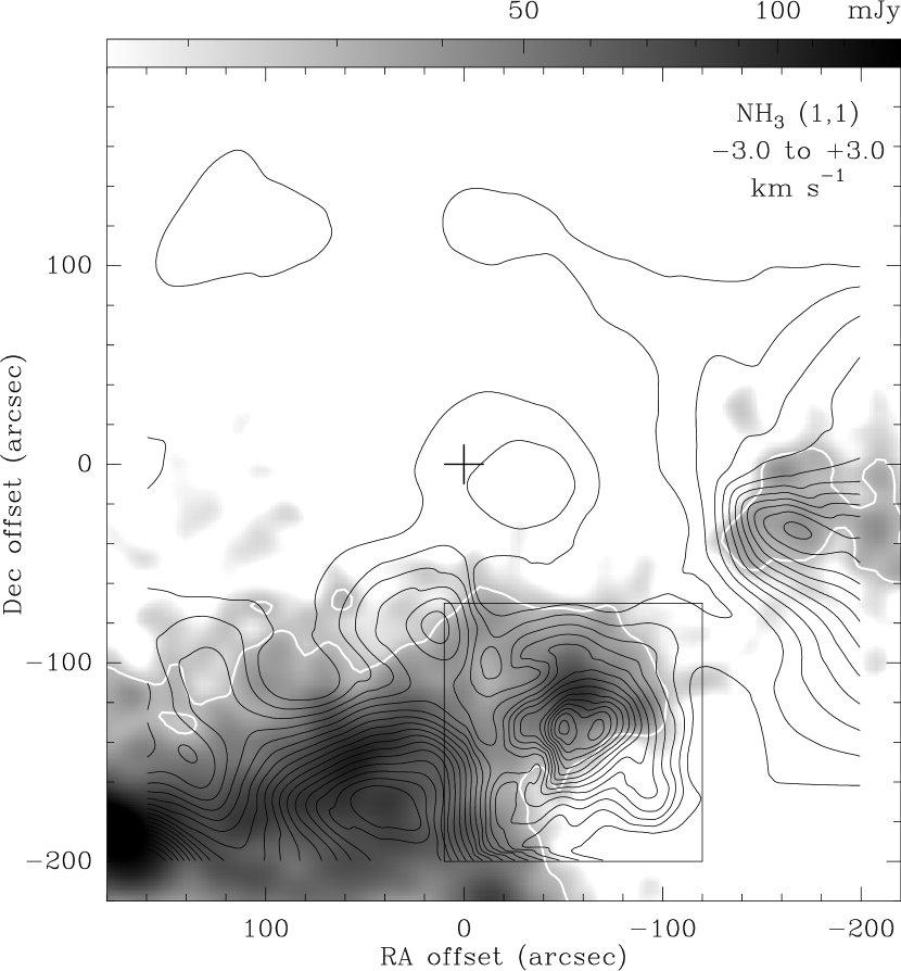
Figure 1: NH₃ (1,1) line intensity map in direction to G79.29+0.46. Only the main component has been integrated, in the velocity range indicated at the top right corner. On grayscale, the 1.2 mm continuum image of the MAMBO cameras at the IRAM 30 m telescope is also plotted (Motte et al. 2007). The logarithmic intensity scale used is indicated in the top bar. NH₃ starting contours and spacing are 0.2 K km s^-1. Equatorial coordinates are referred to the star position (Sect. 2). The region was fully sampled within the square indicated at the south west, and every 40″elsewhere. The white contour, taken from the MAMBO data, is plotted to indicate the boundaries of the IRDC. Most of the NH₃ (1,1) emission seems associated with the cold dust traced by the 1.2 mm continuum, although some low-level features are also noted (see text).

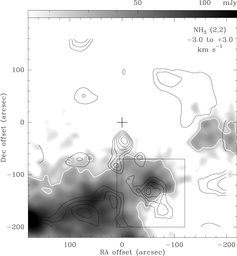
Figure 2: The same as Fig. 1 for the NH₃ (2,2) line. Contours start at 0.22 K km s^-1, and are spaced by 0.11 K km s^-1. Although the most extended emission is well correlated to the dark cloud in the south and west, the peak of the (2,2) line arises from the $(0\arcsec,-40\arcsec)$ position and is not correlated to the 1.2 mm emission.

3 Results

3.1 Overall emission

The whole velocity range of NH₃ emission, from $-3$ km s^-1 to $+3$ km s^-1, falls within the corresponding to Cyg X and the Great Rift regions (Schneider et al. 2006; Gottschalk et al. 2012). Channel maps of the emission of the (1,1) and (2,2) lines are presented in an online appendix, and the spectra are also accessible for download at CDS. The velocity-integrated maps of both lines, in the interval $(-3,+3)$ km s^-1, are shown in Figs. 1 and 2. In Fig. 1, the (1,1) contours are superimposed on the 1.2 mm continuum image from the MAMBO and MAMBO-2 cameras at the IRAM 30 m telescope (Motte et al. 2007), smoothed to an angular resolution of $\sim$26″. The figure shows that the most intense NH₃ and 1.2 mm emission arises from the IRDC, extending from the south-east to the west of our field of view, and consisting of four main clumps. The peaks of ammonia do not agree with those of the 1.2 mm continuum. The SW region (the area inside the square) is the closest in projection to the ring of ionized nebula (Higgs et al. 1994; Umana et al. 2011). It is worth noting that while the southern clump and the SW region are physically connected, the connection between the SW region and the western clump suffers a discontinuity both in dust and gas, even taking into account that their overall structure suggests they are part of the same large-scale cloud. There is also some weak emission, traced by the low-level contours; this low-level emission is particularly visible at the northern and western part of the field, and also close to its centre, near the LBV star.

The NH₃ (2,2) line emission shares some of the (1,1) features. Fig. 2 plots the NH₃ (2,2) emission in the same velocity range as in Fig. 1. Again, the most extended emission appears correlated to the 1.2 mm continuum, and consequently to the IRDC; furthermore, some emission at the centre and the west is also present. It is notable that the peak of the whole map arises from a position close to the LBV star, at $(0\arcsec,-40\arcsec)$. The central part of the field is devoid of NH₃ (2,2) emission, except at the $(0\arcsec,-40\arcsec)$ position.

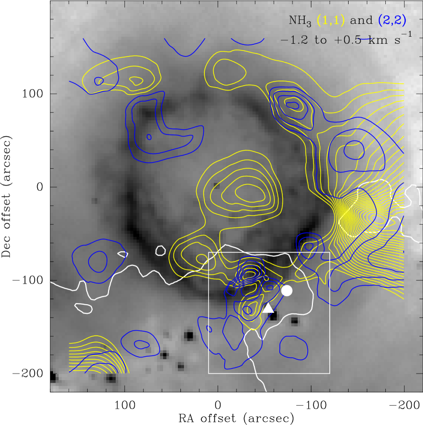
Figure 3: NH₃ (1,1) and (2,2) integrated line emission in the velocity range $(-1.2,+0.5)$ km s^-1, overlaid on the 70 $\mu$m continuum of Herschel/PACS. The white contour is the same depicted in Figs. 1 and 2. The fully sample area is indicated by the white square. The white triangle (circle) points to the position of the NH₃ (CO) peak. NH₃(1,1) starting and spacing contours (yellow) are 0.12 and 0.06 K km s^-1, respectively. NH₃(2,2) starting and spacing contours (blue) are 0.04 K km s^-1. In this velocity range, the ammonia emission is dominated by a ring-like structure towards the outer part of the ring nebula (see text).

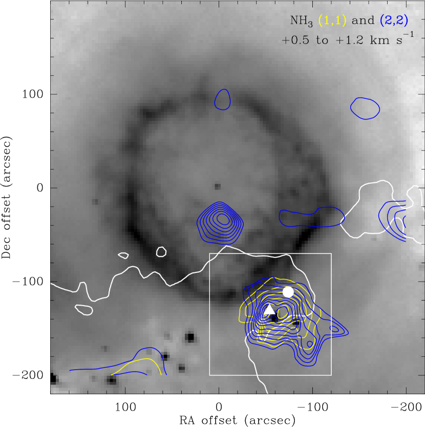
Figure 4: The same as Fig. 3, but for the the velocity range $(+0.5,+1.2)$ km s^-1. Starting contours and spacing of the NH₃ (1,1) line (yellow) are 0.6 K km s^-1 and 0.2 K km s^-1, respectively. For the NH₃ (2,2) line, the starting contours and spacing (blue) are 0.09 and 0.03 K km s^-1, respectively. At this velocity range, the ammonia emission is particularly intense towards the SW region (e.g., within the white square), in coincidence with the most prominent CO emission. Another outstanding feature is the (2,2) spot around $(0\arcsec,-40\arcsec)$, which has no (1,1) counterpart.

3.2 NH₃ associated with the LBV nebula

In order to identify and further characterize the ammonia associated with G79.29+0.46, we have thoroughly studied the NH₃ emission in different velocity bins. After this analysis, two velocity ranges are particularly interesting. In Figs. 3 and 4, the emission of the (1,1) and (2,2) lines are sketched in such velocity intervals.

Figure 3 shows the ammonia emission in the velocity range $(-1.2,+0.5)$ km s^-1, overlaid to a Herschel/PACS image at 70 $\mu$m . An outstanding morphological correlation with the ring nebula (especially in the (1,1) line) is noted in this figure, where a large fraction of the 70 $\mu$m ring is surrounded by an ammonia feature. This NH₃ ring-like structure bounds the 70 $\mu$m ring to the north and west, but is projected above it towards the south. The (2,2) line also shows a similar morphology, although not as clear as the (1,1) line. The lowest-level contours of the (1,1) and (2,2) lines corresponds to a signal-to-noise (S/N) ratio greater than 4 and 1.5, respectively, which explains the lack of a better correlation in the (2,2) line.

Moreover, the inner part of the nebula is also partially filled by (1,1) emission, without a (2,2) counterpart. Due to the undersampling and the limited S/N ratio, it is not possible to determine whether a physical connection between the ammonia ring and the emission at the field centre exists. If so, most of the NH₃ associated with the LBV nebula could be the surviving of a formerly complete NH₃ shell.

Figure 4 is similar to Fig. 3, but covers the second velocity range of interest: $(+0.5,+1.2)$ km s^-1. Here, the NH₃ emission of both lines is concentrated towards the SW region, approximately at the centre of the fully sampled area. The (2,2) line emission also depicts a strong spot around $(0\arcsec,-40\arcsec)$ without a counterpart in the (1,1) line.

The velocity of the NH₃ ring does not match with the values reported for the CO shell (see Figs. 6 and 7 of Jiménez-Esteban et al. 2010), which are around $-3$ km s^-1 and $+3$ km s^-1. This contradictory result is only apparent, because it accounts for intrinsic differences in the molecules under comparison. CO is very abundant and ubiquitous, optically thick and with a low critical density; therefore, it is expected the emission of CO in environments with a wider range of physical conditions than NH₃. The velocity of the NH₃ ring fits well within the whole range of emission associated to the CO shell ($-5$ to $+5$ km s^-1; see Rizzo et al. 2008), but is close to the velocity of the local arm in this direction, and also the velocity of Cygnus X and the Great Cygnus Rift. The velocity ranges of the CO slabs reported by Jiménez-Esteban et al. (2010) are merely those where the confusion effects are minor and a clear correlation with the infrared shell is noted.

In projection, the NH₃ ring bounds the ring nebula and the CO slabs, although the presence of any positional differences between CO and NH₃ should take into consideration the arguments presented above, and the fact that the comparison is made at different velocities. As we discuss below, the lack of ammonia at the ring nebula positions is consistent with the destruction of this molecule by the high UV field.

3.3 NH₃ (3,3) in the SW region

We devoted a special attention to the SW region, because it hosts a multiple layered CO structure (Rizzo et al. 2008; Jiménez-Esteban et al. 2010), and is also claimed as a site of interaction between the LBV nebula and its environs (Umana et al. 2011).

The CO (Rizzo et al. 2008; Jiménez-Esteban et al. 2010) and dust-continuum emission (Figs. 1 and 2) are very well correlated in this region. Ammonia also depicts a strong and compact emission in the SW region, although does not peak at the same position as CO and dust. Hereafter, we will refer to the peaks of emission of ammonia and CO as the “NH₃ peak” and the “CO peak”. The NH₃ peak is near the centre of the SW region, at $\sim(-54\arcsec,-131\arcsec)$, while the CO peak is shifted with respect to the NH₃ peak approximately by $(-20\arcsec,+20\arcsec)$. In order to better analyse these two points, we have done deep integrations of the (3,3) line.

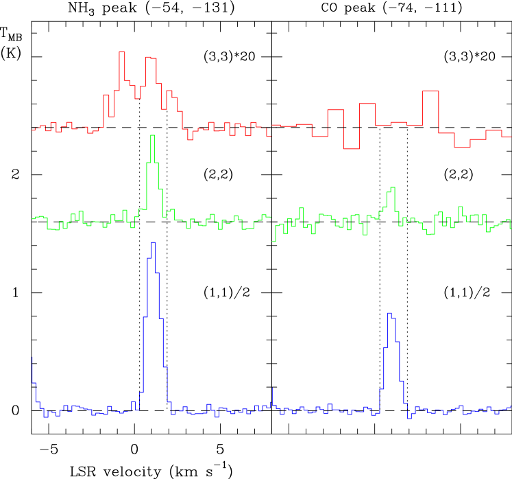
Figure 5: NH₃ (3,3) observations in the south-western part of the field. Two positions (the NH₃ and the CO peaks) have been observed, indicated above the boxes. The (1,1) and (2,2) spectra towards the same positions are also plotted for comparison. Note that the (1,1) intensity scale is reduced by a factor of two, and the (3,3) spectra are multiplied by 20. The (3,3) spectrum towards the CO peak has been smoothed to 0.7 km s^-1. Dashed vertical lines are plotted at $+0.3$ and $+1.9$ km s^-1 to facilitate further comparisons among the lines, and to separate the three components present in the (3,3) line towards the NH₃ peak.

Both (3,3) spectra are presented in Fig. 5, together with the corresponding (1,1) and (2,2) lines. Dashed velocity marks have been added at $+0.3$ and $+1.9$  km s^-1 to facilitate the comparisons.

The first feature in the figure is the lack of (3,3) emission in the CO peak. The ratio of the areas between the NH₃ peak and the CO peak –computed in the velocity range $(+0.3,+1.9)$ km s^-1of the (3,3) line– is greater than 16. On the other hand, the same ratios computed for the (1,1) and (2,2) lines are 1.8 and 2.8, respectively. Therefore, the absence of emission in the (3,3) towards the CO peak is statistically significant.

A second feature in Fig. 5 is the presence of three velocity components in the (3,3) line towards the NH₃ peak. The velocity of the central component, roughly between the velocity marks, agrees with those of the (1,1) and (2,2) lines. However, the lower (blue) and higher (red) velocity components of the (3,3) line do not have any counterpart in the (1,1) or (2,2) line emission. As we analyse below, the blue and red components are characterized by higher temperatures than the central component.

4 Analysis of the NH₃ emission

4.1 Derivation of physical parameters

Ammonia is a rather ubiquitous molecule. Heavily destroyed in the presence of UV fields (e. g. Fuente et al. 1990, and references therein), it is present in cold dark clouds (Jijina et al. 1999; Sepúlveda et al. 2011) and also in regions affected by shocks (Tafalla & Bachiller 1995; Zhang et al. 2002; Palau et al. 2007). Since the very beginnings of molecular spectroscopy, it has been largely recognized as an excellent thermometer of the ISM (Ho & Townes 1983; Guesten et al. 1985; Maret et al. 2009).

From the joint analysis of the (1,1) and (2,2) metastable lines, we have derived several physical properties of the NH₃ gas. The details of the formulation are explained in an online appendix. This analysis was done at each position with significant emission ($>3\sigma$) in any of the two lines.

The (1,1) line emission arising from the IRDC is mostly optically thick, and the opacities were estimated through a hyperfine (hf) fitting. No satellite lines were detected elsewhere, and only a Gaussian fitting were done. All the positions with significant emission in the (2,2) line were also fitted by Gaussian profiles.

To estimate the ammonia abundance, $X($NH₃$)$, we have used the 1.2 mm map of Motte et al. (2007) and computed the H₂ column density following Motte et al. (1998). Assumptions and formulation are also exposed in the Appendix.

In the NH₃ peak of the SW region, where the (3,3) line was observed and detected, we proceeded with a Boltzmann diagram approach to determine the rotational temperature and column densities of the three velocity components. The procedure is also described in the Appendix.

4.2 Rotational and kinetic temperatures

The distribution of the rotational temperatures ($T_{\mathrm{rot}}$) is sketched in Fig. 6. The values are written at their corresponding positions, superimposed to a Spitzer image at 8 $\mu$m.

The blue labels correspond to the points where the hf fitting was possible. All these positions belong to the IRDC (as said above), and are characterized by a very low and uniform $T_{\mathrm{rot}}$, in the range $7-11$ K. The points having two values of $T_{\mathrm{rot}}$ correspond to those cases where two velocity components were fitted.

The yellow labels correspond to those points with both lines fitted by Gaussian profiles, and with derived values of $T_{\mathrm{rot}}$ lower than 40 K. In case of non-detection of the (2,2) line, the values are expressed as upper limits. None of these points are correlated to the IRDC, and it is hard to establish a tendency across the observed field.

The red labels correspond to those positions where the (1,1) line remains undetected, and therefore the values of $T_{\mathrm{rot}}$ are lower limits. These “hot spots” are spread over the whole observed field, but again avoiding the IRDC positions. As the hot spots are located in the under-sampled area, we have to interpret them as small regions (less than $40\arcsec$) with special local conditions. The peak of the (2,2) line in Fig. 4 –offset $(0^{\prime\prime},-40^{\prime\prime})$– has a lower limit of $T_{\mathrm{rot}}$ of 63 K.

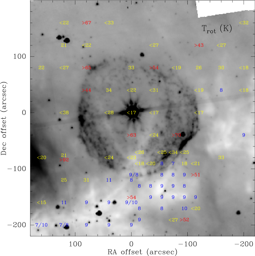
Figure 6: Distribution of the rotational temperatures, overlaid to the 8 $\mu$m image of Spitzer. The values derived from hyperfine fitting of the (1,1) line are labelled in blue; those derived from Gaussian fitting of both lines are shown in yellow; red labels correspond to those positions having the highest values of $T_{\mathrm{rot}}$ (see text). In all cases, fitting of the (2,2) has been obtained with a single Gaussian component. The low temperatures associated with the IRDC, and higher values elsewhere are clearly revealed.

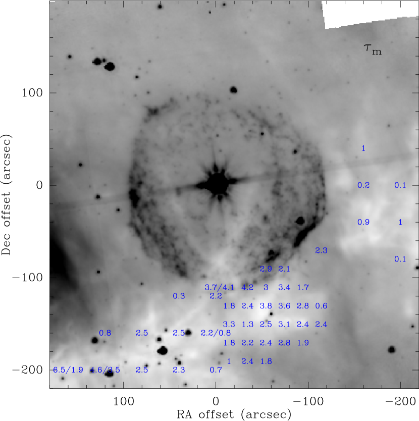
Figure 7: Distribution of the opacities, in all the positions where a hyperfine fitting of the (1,1) line was possible, i. e. mostly in the IRDC.

Figure 8: Distribution of the ammonia column density, in units of $10^{12}$  cm^-3. Colour are the same as Fig. 6. Details about the computation of $N($NH₃$)$ are provided in the text. It is remarkable the large difference between the IRDC and the other positions (see text).

The general picture of the region consists, therefore, of a very cold and massive IRDC, spotted by tenuous areas, some of them depicting moderately high temperatures. This strong difference in the temperatures among the IRDC and the other positions is even larger if we consider the kinetic temperatures ($T_{\mathrm{k}}$), because the ratio between $T_{\mathrm{k}}$ and $T_{\mathrm{rot}}$ increases with $T_{\mathrm{rot}}$ (Danby et al. 1988; Tafalla et al. 2004). At the IRDC, $T_{\mathrm{k}}$ is in the range $8-12$ K, while the positions having yellow labels may have $T_{\mathrm{k}}$ between 25 and 47 K. It is hard to constrain $T_{\mathrm{k}}$ in the hot spots, although large values, 100 K or even more, are possible.

4.3 Opacities in the IRDC

Fig. 7 depicts the opacities of the main group ($\tau_{m}$ in the appendix), derived when the hf fitting is possible. The positions correspond to the IRDC, and are labelled in blue, as in Fig. 6. Positions having two opacities correspond to those cases with two velocity components. As expected in the case of dark clouds, the larger opacities are found toward the inner part of the IRDC. A notable exception is found in the SW region, where the opacity remains high in the northern edge of the region, close to the border of the ring nebula.

4.4 Column densities and abundances

Fig. 8 depicts the distribution of the column density, $N($NH₃$)$, in the observed field. The colour code is the same as in Fig. 6. The estimates of $N($NH₃$)$ in those hot spots (red labels) where only lower limits to $T_{\mathrm{rot}}$ are determined, was done by assuming $T_{\mathrm{rot}}$ = 50 K; all lower limits to $T_{\mathrm{rot}}$ are higher than 50 K and, therefore, the values of $N($NH₃$)$ are lower limits in all these cases. At the positions where we determined upper limits (yellow labels), we assumed $T_{\mathrm{rot}}$ = 10 K. In those cases having two velocity components, the sum of both $N($NH₃$)$ are depicted.

After looking at the Fig. 8, the differences between the IRDC and the rest of the field are outstanding. $N($NH₃$)$ varies from several $10^{14}$ to some $10^{16}$  cm^-3 at the IRDC positions, and is in the range from $10^{12}$ to $10^{13}$  cm^-3 elsewhere.

This ample range of the $N($NH₃$)$ values also affects the estimates of abundances with respect to H₂, $X($NH₃$)$. Fig. 9 shows the $X($NH₃$)$ distribution in the field, with the same colour codes as previous figures. To compute the NH₃ abundance, we had to estimate the H₂ column density ($N($H₂) at all positions. This is inferred from the 1.2 mm continuum, considered a dust tracer. Assumed dust temperatures were 10 K at the IRDC positions and 50 K elsewhere (see the appendix for details about the criteria used.

The lowest values of the abundances, in the range from several $10^{-11}$ to some $10^{-9}$, are spread all along the observed field except in the IRDC, where the abundance grows up to some $10^{-8}$. Interestingly, the abundance in the SW region remains high at its northern and south-western borders. This is not the tendency expected in a quiescent clump of a dark cloud like, for instance, the other clumps of the IRDC.

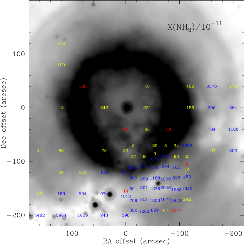
Figure 9: Distribution of the ammonia abundances, in units of $10^{-11}$ overlaid to an image of Spitzer/MIPS at 24 $\mu$m to highlight the second infrared ring. See details of the computation of H₂ column densities in the text. Notable differences between the IRDC and the rest of the field are again noted; furthermore, high values appear in the northern and south edges of the SW region, coinciding with the position of the first and second infrared rings, respectively (see text).

4.5 The NH₃ peak

In Fig. 10, we show the Boltzmann diagram of the NH₃ peak after fitting the (3,3) spectrum to three Gaussian velocity components. The velocity ranges and the velocity-integrated line intensities of the fitting are shown in Table 1. We named the components as central, blue and red according to their velocity ranges.

Table 1: Boltzmann diagram results in the NH₃ peak

Component	velocity range	$T_{\mathrm{rot}}$	$N($NH3$)$
	km s-1	K	cm-2
Central	$(+0.3,+1.9)$	$11\pm 2$	$1.7\pm 0.2\ 10^{15}$
Blue	$(-1.7,+0.3)$	$>40$	$<1.5\ 10^{12}$
Red	$(+1.9,+2.8)$	$>28$	$<1.5\ 10^{12}$

As said above, the (1,1) and (2,2) lines have not been detected in the red or blue velocity components; in these cases, upper detection limits (3-sigma) have been computed in the corresponding velocity ranges.

The results of the Boltzmann diagram are shown in the last two columns of Table 1. $T_{\mathrm{rot}}$ and $N($NH₃$)$ can be determined only for the central component. For the others, we only derived lower limits of $T_{\mathrm{rot}}$. As we also considered the column densities up to the first four metastable levels (see Appendix), the resultant values of $N($NH₃$)$ are therefore upper limits.

Most of the gas (of the order of $10^{15}$ cm^-2) arises in the central component and has a low value of $T_{\mathrm{rot}}$ (11 K); these values of $T_{\mathrm{rot}}$ and $N($NH₃$)$ are those typically measured in the IRDC.

But strikingly, there is much low amount of gas (three orders of magnitude lower) at higher temperatures, above 28 K and 40 K. This finding confirms the scenario depicted by the (1,1) and (2,2) lines in the whole field: most of the dense gas is in cold form and associated with the IRDC, which in turn is embedded in a field dotted by low amounts of warm/hot gas.

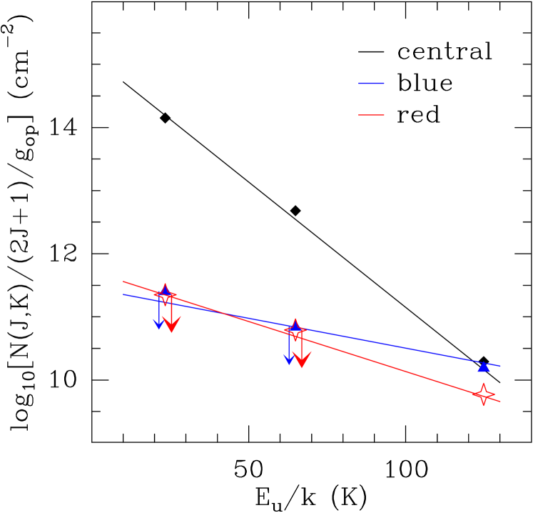
Figure 10: Rotational diagram corresponding to the NH₃ peak. The column densities have been computed for the three velocity components depicted in Fig. 5, also indicated in Table 1. The best-fit lines are sketched. The rotational temperature is only determined for the central component, while for the others (blue and red) only lower limits can be derived.

4.6 Anomalous NH₃(1,1) spectra in the SW region

We found anomalous satellite ratios in the NH₃(1,1) spectra at four positions of the SW region. Figure 11 shows the spectra, together with their locations. The positions affected by this anomalous emission lie at the outer edges of the SW region, two of them close to the CO peak.

The blue outer satellite hyperfine components are stronger than those of the red side. This has been proposed to be a signpost of contracting motions, both theoretically (Park 2001) and observationally (e. g. Fontani et al. 2012).

Alternatively, the anomaly could be due to non-LTE emission due to hyperfine selective photon trapping, as this affects only the outer satellites. However, this effect would produce the opposite result; the red satellite would become stronger than the blue one (Stutzki & Winnewisser 1985).

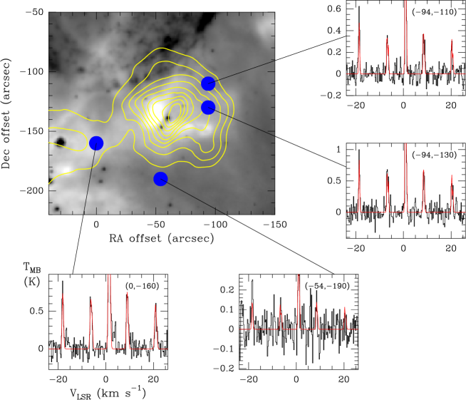
Figure 11: Anomalous spectra in the SW region. The grey scale displays the Spitzer/IRAC 8 $\mu$m emission, and the yellow contours the NH₃ (1,1) integrated emission. Blue dots mark the positions of the anomalous spectra. These spectra are shown in the smaller boxes outside the map. Offsets are indicated on the top right corner of each spectrum. The observed spectra are in black and the fitting in red. The $T_{\mathrm{MB}}$ scale has been chosen to improve the visibility of satellite lines.

5 Discussion

5.1 Critical revision of the distances

The most recent distance estimate to some star-forming regions of Cygnus X is 1.4 kpc, based on spectroscopic parallaxes of their maser-emitting regions (Rygl et al. 2012). This distance is only slightly smaller than previous estimates using the same technique (Torres-Dodgen et al. 1991), and consistent with other works based on stellar classification (e. g. Hanson 2003). On the other hand, several studies locate DR15 at a lower distance, about 700-800 pc (Wendker et al. 1991; Uyanıker et al. 2001; Redman et al. 2003).

However, the distance to the IRDC is still a matter of debate, with distances ranging from 800 to 1700 pc (Redman et al. 2003; Kraemer et al. 2010). A close inspection of the infrared images and submillimeter continuum emission of a large field of view ($20^{\prime}\times 20^{\prime}$) including G79.29+0.46 reveals that the IRDC is interrupted in two positions: the SW region (e. g. Kraemer et al. 2010; Jiménez-Esteban et al. 2010; Umana et al. 2011), and the position of DR15 (see Fig. 2 of Redman et al. 2003). At first sight, the IRDC is farther away than both DR15 and the LBV nebula. However, the presence of a dark filamentary structure extending to the north of the IRDC and crossing the LBV nebula up to the position of the LBV star suggests that part of the IRDC is also in front of the LBV nebula (Figs. 6, 7, 8, and 11). Therefore, provided that part of the IRDC seems to be in front of the LBV nebula, and part of it seems to be behind, it seems reasonable to consider that the IRDC and the LBV nebula lie at similar distances, of 1.4 kpc.

In addition, the overall NH₃ (1,1) and 1.2 mm emission shown in Fig. 1 reveal a discontinuity separating the SW region and the westernmost clump of the IRDC, which is coincident with a bright 8 $\mu$m structure extending from the infrared ring farther to the south-west (Figs. 6, 7, 8, and 11). This has been proposed as an interaction zone of the LBV star with the surrounding medium (Umana et al. 2011) and favours the association of the LBV star with the IRDC.

The finding of hot spots with low column density in the field of view toward G79.29+0.46 leads us to associate the most tenuous ammonia to the Cygnus X star-forming region, or even to G79.29+0.46 itself. In this scenario, the warm/hot spots may represent the relics of the clumps of the ancient molecular cloud, which are being photo-evaporated by the UV field from G79.29+0.46, perhaps supported by other neighbouring massive stars. This idea is reinforced by the low abundance of NH₃ measured near G79.29+0.46, compatible with the idea of NH₃ being photo-dissociated by the strong UV radiation present in the region. The high temperatures found in the nebula are consistent with the high dust temperature already found in the same region (Waters et al. 1996; Jiménez-Esteban et al. 2010).

In summary, we are providing here sufficient arguments which favour the possibility of some co-existence of the IRDC and G79.29+0.46 in close volumes. Therefore, the interplay between these two objects should be explored in more detail.

5.2 Hints of a possible interaction in the SW region

As said above, the fraction of the IRDC which we mapped is roughly divided in four regions, more or less aligned from the south-east corner of the map to its western border. In some aspects, the SW region (one of these four regions) presents a number of peculiarities as compared to the other three regions.

The opacities measured in the SW region do not clearly decrease at the borders, which is not the expected behaviour in a typical cold dark cloud. In particular, the opacity in the northern edge –roughly a strip from $(0",-120")$ to $(-80",-100")$– remains as high as in the centre. The abundance is also high in some points of the same strip, up to one order of magnitude larger compared to the NH₃ peak (located at the centre of the SW region). The southern border –a strip from $(-30",-200")$ to $(-120",-150")$– also depicts some points of high relative abundance. The anomalous (1,1) satellite emission (Sect. 4.6) in the external parts of the SW region is also another peculiarity.

The large differences in some parameters of the SW region, in comparison to the rest of the IRDC, should be due to different physical conditions. An increase of the abundances towards the borders is not the expected tendency in the parts of a cold cloud most exposed to external UV radiation. The abundance of NH₃ in a harsh environment may be enhanced by sputtering in the presence of a C-type shock (Flower & Pineau des Forêts 1994; Draine 1995), which releases volatile molecules from the surface of the dust grains. This is a reasonable hypothesis taking into account the presence of a low-velocity shock (about 14 km s^-1) at the north-western side of the SW region, close to the CO peak (Rizzo et al. 2008). It is also worth noting that the northern edge of the SW region coincides with a brightening and morphological disturbance of the 6-cm continuum emission, which is claimed as an evidence of some interaction with the surrounding ISM (Umana et al. 2011). Therefore, these ammonia observations may have unveiled the molecular counterpart of such disturbance, and also a new molecular component associated with the shocks discovered in CO (Rizzo et al. 2008).

The positions of abundance enhancement towards the southern border of the SW region agree with those of the external infrared shell, better seen in 24 $\mu$m (Jiménez-Esteban et al. 2010, and Fig. 9 of this work).

The scenario of the LBV star interacting with the IRDC is also consistent with the (3,3) spectrum towards NH₃ peak, which reveals two velocity components tracing gas at temperatures $\gtrsim 30$ K, clearly larger than the typical temperatures measured in the IRDC, of $\sim 10$ K.

Therefore, a number of observational findings points to a possible interaction of the nebula and the nested molecular shells with the SW region. A definitive evidence will come from observations with high angular resolution.

5.3 Triggered star formation in the SW region

If the LBV star is interacting with the SW region this could affect the star formation which is currently ongoing in the area (Vink et al. 2008). The dynamical time scale of the ejection events which produced the CO and infrared nested shells is $10{{}^{4}}$–$10{{}^{5}}$ yr (Rizzo et al. 2008; Umana et al. 2011). This is comparable to the age of the brightest young stellar object embedded in the SW region, assuming it is in the Class 0 phase (Greene et al. 1994; Kenyon & Hartmann 1995; Enoch et al. 2009; Evans et al. 2009). Thus, while it seems unlikely that the ejection events of the LBV could have triggered the collapse of the young stellar objects embedded in the SW region, an interesting possibility would be to explore whether they are affecting the formation and evolution of the young stellar objects already formed.

After some $10^{4}-10^{5}$ yr of evolution, G79.29+0.46 will become a Wolf-Rayet star and the NH₃ ring will eventually disappear. The stellar wind regime will change at this stage, turning it out to higher velocity and lower wind density (Langer et al. 1994; Maeder & Meynet 1994; Garcia-Segura & Mac Low 1995). This will produce new shocks in the surrounding gas and dust, which may release volatile molecules from the icy grain mantles (Flower & Pineau des Forêts 1994) and consequently increase the ammonia abundance again. This line of reasoning is supported by the significantly high NH₃ abundance seen to the north and south-western borders of the SW region, a trend also found in the molecular cloud around the WR nebula NGC 2359 (Rizzo et al. 2001a), and the Galactic Center (Flower et al. 1995; Martín-Pintado et al. 1999). The young stellar objects formed in the SW region will probably suffer photo-evaporation and heating of their envelopes.

6 Conclusions

In order to study the molecular gas in the infrared ring nebula of the LBV star G79.29+0.46 and its nearby IRDC, we used the Effelsberg telescope to map the NH₃ (1,1) and NH₃(2,2) emission in the G79.29+0.46 field. We additionally observed NH₃(3,3) in particular positions of the strongest NH₃(1,1) emission. Our main findings are summarized as follows:

1. While the strongest emission of NH₃ (1,1) and (2,2) matches the infrared-dark structure of the IRDC, mainly detected at velocities $>1$ km s^-1, the emission in the velocity range from $-1.2$ km s^-1 to $+0.5$ km s^-1 reveals a coherent structure closely following the infrared ring surrounding the LBV star, also partially seen in the (2,2) transition. This is the first NH₃ structure associated with an evolved massive star known so far.

2. We derived the rotational temperature and NH₃ column density of the dense gas in the entire field of view, and found that the rotational temperature is uniform and in the range 7–11 K in the IRDC, while it is $>30$ K in particular positions or hot spots of the infrared ring nebula and a couple of points within $30^{\prime\prime}$ of the LBV star. The NH₃ column density in the IRDC is in the range 10¹⁴–10¹⁵ cm^-2, while it is about two orders of magnitude lower near the LBV and the infrared ring. Using the 1.2 mm continuum emission in the field, we inferred NH₃ abundances of about 10^-8 in the IRDC, and 10^-10–10^-9 near the LBV star. The warm temperatures and low abundances of NH₃ near the LBV star and its infrared-ring suggest that the gas is being heated and photo-dissociated by the intense UV-field of the LBV star.

3. An outstanding region is recognized beyond the ring nebula towards its south-western part, which is also part of the IRDC (the SW region). The NH₃ (3,3) emission towards the centre of the SW region reveals three velocity components. One of them is associated with the IRDC and has a rotational temperature of 11 K, while the other two are associated with small dense cores with temperatures $>30$ K. In the northern edge of the SW region, the opacity of the (1,1) line keeps a value as high as in the clump centre. The NH₃ abundance tends to be higher at the clump edges than in the clump centre. All these features, together with the results of previous works reporting a shock within this region and hints of interaction with the LBV star, strongly suggests that a mass-loss ejection event of the LBV star is interacting with the SW region and releasing NH₃ molecules back to the gas phase, thus increasing its abundance at the outer edges of the clump.

G79.29+0.46 is providing increasing evidences of being an excellent laboratory to study the history of a high-mass star evolution. Being LBVs the precursors of core-collapse supernovae (through a Wolf-Rayet stage), the knowledge of the different actors present in this field may also help to learn about this topic. The ammonia ring-like structure associated to G79.29+0.46 and the SW region deserve follow up observations with high angular resolution. Furthermore, the observation of other molecular tracers would be of particular interest.

Appendix A Channel maps

The proper channel maps of the two ammonia lines observed are presented in Figs. A.1 and A.2. The collection of spectra are also available at CDS.

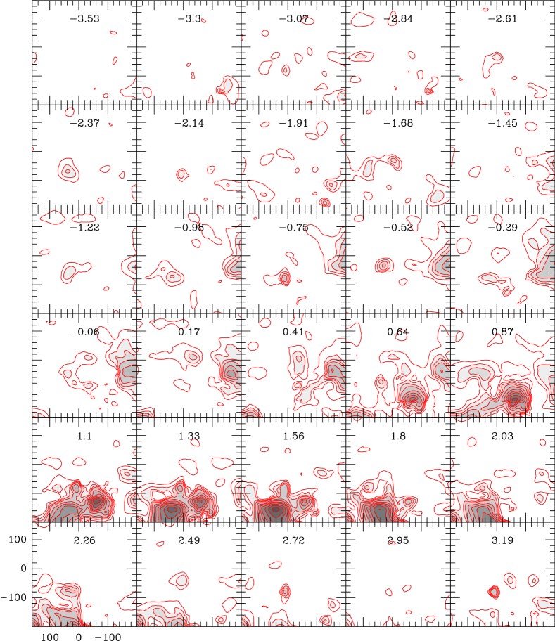
Figure 12: Channel maps corresponding to the NH₃ (1,1) emission. Only the main hyperfine component is depicted. LSR velocities are indicated at the top center of each map. Contours are 0.15, 0.30, 0.45, 0.60, 0.90, 1.20, 1.50, 1.80, 2.25, 2.70, 3.15, 3.60, 4.20, and 4.8 K.

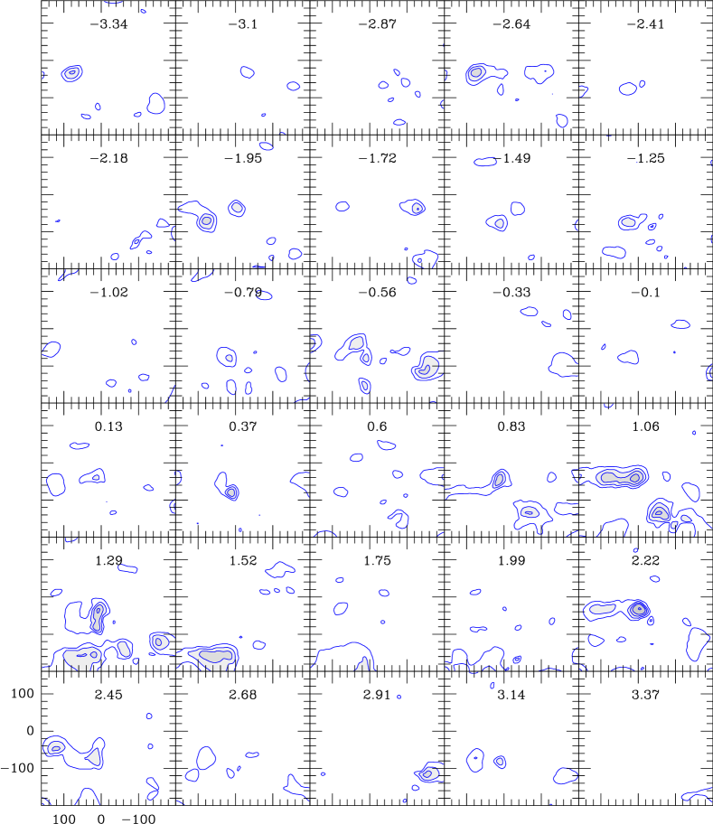
Figure 13: Channel maps corresponding to the NH₃ (2,2) emission. Only the main hyperfine component is depicted. LSR velocities are indicated at the top center of each map. Contours are 0.18, 0.36, 0.54, 0.72, and 1.08 K.

Appendix B Formulation

In this appendix we summarize the formula used for the determination of some physical properties (opacities, rotational temperatures, column densities, and abundances) from the observed NH₃ lines. This corresponds to the standard interpretation already discussed and presented by several authors, such as Ungerechts et al. (1986) and Busquet et al. (2009).

B.1 Hyperfine and Gaussian fitting

The NH₃ lines are splitted by the quadrupole hyperfine interaction (Ho & Townes 1983). From the relative intensities of the main hf group and the four satellite ones, it is possible to directly derive the optical depth of the main hf group (Pauls et al. 1983). When the satellite (1,1) lines are detected, a CLASS method was used for this fitting. The output are: (1) $A\,\tau_{\mathrm{m}}=f\,[J_{\nu}(T_{\mathrm{exc}})-J_{\nu}(T_{\mathrm{bg}})]\,\tau_{\mathrm{m}}$; (2) LSR velocity ($V_{\mathrm{LSR}}$); (3) line width at half maximum ($\Delta v$); and (4) $\tau_{\mathrm{m}}$, the opacity of the main hf group. $f$ is the beam filling factor, and $J_{\nu}(T)$ is Rayleigh-Jeans temperature, defined as $J_{\nu}(T)=({\mathrm{h}}\,\nu/{\mathrm{k}})\leavevmode\nobreak\ (e^{{\mathrm{h}}\,\nu/{\mathrm{k}}\,T}-1)^{-1}$, $T_{\mathrm{bg}}$ = 2.73 K is the background temperature, and h and k are the Planck and Boltzmann constants, respectively.

This formulation assumes that all the hf levels are populated according to local thermodynamic equilibrium (LTE) conditions, and a Gaussian velocity distribution. The level population is characterized by the excitation temperature $T_{\mathrm{exc}}$, which can be cleared from the fitting by:

$$T_{\mathrm{exc}}=\frac{{\mathrm{h}}\nu/{\mathrm{k}}}{ln[1+{\mathrm{h}}\nu/{\mathrm{k}}\ \ W^{-1}]}\,,$$ (1)

where $W=J_{\nu}(T_{\mathrm{exc}})=A/f+J_{\nu}(T_{\mathrm{bg}})$.

The column density of a NH₃ $(J,K)$ level, $N(J,K)$, is obtained by:

$$N(J,K)=\frac{1.65\,10^{14}}{\nu}\ \frac{J(J+1)}{K^{2}}\ \Delta v\ T_{\mathrm{exc}}\ \tau_{\mathrm{tot}}\ \mathrm{cm}^{-2}\,,$$ (2)

where $\nu$ is the line frequency in GHz, $\tau_{\mathrm{tot}}$ is the “total” opacity of all the hf components, and $\Delta v$ and $T_{\mathrm{exc}}$ are in  km s^-1 and K, respectively. The above equation results from solving the Transport Equation for the NH₃ molecule (Wilson et al. 2009), using a dipole moment $\mu=1.469$ D, and assuming $T_{\mathrm{exc}}$ $>>$ $T_{\mathrm{bg}}$.

When the hyperfine fitting is possible, we estimate the column density of the (1,1) level, N(1,1), using the above equation. Numerically, it is computed by:

$$N(1,1)=2.785\ 10^{13}\ \Delta v\ T_{\mathrm{exc}}\ \tau_{\mathrm{m}}\ \mathrm{cm}^{-2}\,,$$ (3)

where a rough assumption of $\tau_{\mathrm{tot}}=2\ \tau_{\mathrm{m}}$ is used.

When the hyperfine fitting is not possible, we have assumed optically thin emission. In this case, Eq. (B.2) for the (1,1) line turns out to:

$$N(1,1)=1.308\ 10^{13}\ \int{T_{\mathrm{MB}}\ dv}\ \mathrm{cm}\,^{-2}\,.$$ (4)

In the above equation, all the hf components are included in the integral. If the integration extends only to the main group, the coefficient should then be multiplied by a factor of 2.

In the case of the (2,2) line, the equivalent expression is:

$$N(2,2)=9.801\ 10^{12}\ \int{T_{\mathrm{MB}}\ dv}\ \mathrm{cm}\,^{-2}\,.$$ (5)

Provided $N(1,1)$ and $N(2,2)$, the rotational temperature $T_{\mathrm{rot}}$ can be computed (Townes & Schawlow 1975; Ho & Townes 1983) by:

$$T_{\mathrm{rot}}=\frac{-41.5}{ln\left(\frac{3}{5}\,\frac{N(2,2)}{N(1,1)}\right)}\leavevmode\nobreak\ {\mathrm{K}}\,,$$ (6)

which results from a two-level system approximation (Ho & Townes 1983).

The partition function is given by

$$\begin{array}[]{rrl}Q(T)&\!\!\!=\!\!\!&\sum\limits_{J,K}\ g_{JK}\ e^{-E_{JK}/\mathrm{k}T}\\ \\ &\!\!\!\approx\!\!\!&1+3\,e^{-23.4/T}+5\,e^{-64.9/T}+14\,e^{-124.8/T}\,,\end{array}$$ (7)

where $g_{JK}=(2J+1)\,g_{op}$ and $E_{JK}$ are the statistical weight and the energy of the level $(J,K)$, and $g_{op}$ is the statistical weight for the ortho and para species. In the above equation we summed up to the first four levels  , and assumed that (1) only the metastable levels are populated; (2) the levels are characterized by the LTE temperature T; and (3) $g_{op}$ equals to 2 and 1 for the ortho and para species, respectively.

The total column density of all the metastable lines may be computed from a single line and by assuming a partition function characterized by $T$ = $T_{\mathrm{rot}}$(e. g. Ungerechts et al. 1986; Busquet et al. 2009):

$$N(\mathrm{NH}_{3})=\left(N(J,K)/g_{JK}\right)\ Q(T_{\mathrm{rot}})\ e^{E_{JK}/\mathrm{k}T_{\mathrm{rot}}}.$$ (8)

In particular, for the (1,1) line the above equation becomes

$$N(\mathrm{NH}_{3})=N(1,1)\left[\frac{1}{3}e^{23.4/T_{\mathrm{rot}}}+1+\frac{5}{3}e^{-41.5/T_{\mathrm{rot}}}+\frac{14}{3}e^{-101.2/T_{\mathrm{rot}}}\right].$$ (9)

When the (2,2) line is the only one detected, an equivalent formula to (B.9) is:

$$N(\mathrm{NH}_{3})=N(2,2)\left[\frac{1}{5}e^{64.9/T_{\mathrm{rot}}}+\frac{3}{5}e^{41.5/T_{\mathrm{rot}}}+1+\frac{14}{5}e^{-59.6/T_{\mathrm{rot}}}\right].$$ (10)

B.2 Abundances

The NH₃ abundance is computed by

$$X(\mathrm{NH}_{3})=N(\mathrm{NH}_{3})/N(\mathrm{H}_{2})\,,$$ (11)

where $N($H${}_{2})$ is the H₂ column density. To estimate it, we used the survey of the Cygnus region done by Motte et al. (2007) in the 1.2 mm continuum emission.

At this wavelength, most of the flux arises from thermal dust emission, which is optically thin. By assuming a constant gas-to-dust ratio, the 1.2 mm flux results directly related to the total gas. We therefore used the formulation of Motte et al. (1998), accordingly adapted to our case.

More precisely, we have used their Eq. (1’), which compute $N($H${}_{2})$ as a function of the 1.2 mm flux, the dust temperature ($T_{\mathrm{dust}}$) and $\kappa_{\mathrm{1.2mm}}$, the dust opacity per unit mass column density.

The map of Motte et al. (2007) was convolved to 40″ in order to match the 100m’s angular resolution. For $\kappa_{\mathrm{1.2mm}}$ we have adopted a value of 0.01 g^-1 (cm^-2)^-1, which corresponds to the case of dust particles covered by thin ice mantles (Ossenkopf & Henning 1994), and is also a geometrical average between the values usually adopted for pre-stellar dense clumps and circumstellar envelopes in young stellar objects of class II (Motte et al. 2007).

Under these assumptions, the resulting formula is

$$N({\mathrm{H}}_{2})\approx 2\,10^{20}\leavevmode\nobreak\ S({\mathrm{mJy}})\leavevmode\nobreak\ \left(\frac{T_{\mathrm{dust}}}{20\,{\mathrm{K}}}\right)^{-1}\leavevmode\nobreak\ {\mathrm{cm}}^{-2}\,,$$ (12)

where $S$ is the flux at 1.2 mm in the convolved map. $T_{\mathrm{dust}}$ is assumed as 10 K in the IRDC positions, and 50 K elsewhere, consistent with the two dust population previously reported in the region (Umana et al. 2011).

For the IRDC, the assumed value of 10 K is compatible with the $T_{\mathrm{rot}}$ derived from the hf fitting, because $T_{\mathrm{k}}$$\approx$$T_{\mathrm{rot}}$ at low temperatures, and the gas is thermalised at the dust temperature. At the other positions –particularly in the ring nebula and its interior– the continuum emission is bright at shorter wavelengths, such as 24 $\mu$m, indicating a dust temperature probably larger. By assuming a conservative value of 50 K the derived values of $N($H${}_{2})$ have to be considered as upper limits and thus $X($NH₃$)$ as lower limits.

B.3 Rotational diagrams

The rotational diagram, also known as the Boltzmann diagram approach, is a rather common methodology used to derive the rotational temperature and column density of a given species. The method is described in many works (see, for example, Goldsmith & Langer 1999) and assumes a population of the levels characterized by $T_{\mathrm{rot}}$, under LTE conditions.

By taking logarithms to Eq. B.8, and after some algebra, we obtain:

$$\log\left[N(J,K)/g_{JK}\right]=-\frac{\log e}{T_{\mathrm{rot}}}\ \left(E_{JK}/\mathrm{k}\right)+\log\left[N(\mathrm{NH}_{3})/Q(T_{\mathrm{rot}})\right]\,.$$ (13)

We see in the above equation that the energy of the upper levels are linearly related to the logarithms of the column densities.

If three or more lines of a given species are measured, we can define the abscissa $x$ as $\left(E_{JK}/\mathrm{k}\right)$, and the ordinate $y$ as $\log\left[N(J,K)/g_{JK}\right]$. $x$ and $y$ are related by the usual linear equation $y=a\,x+b$, and we can therefore find the least square regression line. $T_{\mathrm{rot}}$ and $N($NH₃$)$ can be obtained from the slope $a$ and the constant term $b$ by:

$$T_{\mathrm{rot}}=-\log e/a$$ (14)

and

$$N(\mathrm{NH}_{3})=10^{b}\ Q(T_{\mathrm{rot}})\,.$$ (15)